Ensemble Transfer Learning for Distinguishing Cognitively Normal and Mild Cognitive Impairment Patients Using MRI

Abstract

Alzheimer’s disease is a chronic neurodegenerative disease that causes brain cells to degenerate, resulting in decreased physical and mental abilities and, in severe cases, permanent memory loss. It is considered as the most common and fatal form of dementia. Although mild cognitive impairment (MCI) precedes Alzheimer’s disease (AD), it does not necessarily show the obvious symptoms of AD. As a result, it becomes challenging to distinguish between mild cognitive impairment and cognitively normal. In this paper, we propose an ensemble of deep learners based on convolutional neural networks for the early diagnosis of Alzheimer’s disease. The proposed approach utilises simple averaging ensemble and weighted averaging ensemble methods. The ensemble-based transfer learning model demonstrates enhanced generalization and performance for AD diagnosis compared to traditional transfer learning methods. Extensive experiments on the OASIS-3 dataset validate the effectiveness of the proposed model, showcasing its superiority over state-of-the-art transfer learning approaches in terms of accuracy, robustness, and efficiency.

1. Introduction

Alzheimer’s disease (AD), the most common form of dementia, poses a significant challenge to healthcare providers. It causes a progressive, irreversible brain disorder characterised by a deterioration of cognitive functions. In the United States, Alzheimer’s disease is the fifth leading cause of death among adults age 65 and older, and there was a 145% increase in deaths from Alzheimer’s disease in 2017 [1]. Recently, a significant amount of research [2,3,4,5,6] has been conducted in order to detect early and pre-symptomatic stages of AD to slow or prevent the progression of the disease. Surprisingly, simple cognitive assessments of dementia were only accepted by a minority of the older adults. In particular, techniques based on MRI testing have been developed and used to identify AD [5]. The accuracy of an AD diagnosis mostly depends on the biomarkers of the disease. The features to detect Alzheimer are extracted from the region of interest (ROI) of the brain which has the potential to contain the tissue that are sensitive markers for dementia. Similarly, the distinctive features are confirmed by the histopathology of dementia that display these ROI in the amygdala and hippocampus embedded deep into the temporal lobe of the brain [7,8]. Due to the recent advancements in automating the prediction of early diagnosis of dementia, the objective has shifted to help non-experts and non-neurologist users to identify early signs of AD.

AI-based computer-aided diagnosis (CAD) has become a feasible and a popular tool in medicine due to its low cost and transparent decision making [9,10,11,12]. Traditional methods of feature extraction require handcrafted features [13,14,15,16]. Castellazzi et al. [17] combined advanced qMRI measurements along with conventional machine learning techniques to classify AD from Vascular Dementia (VD) and investigated if the suggested method might be used to forecast the common illness in those who do not have distinct AD or VD profiles. In the work proposed by Battineni et al. [18], four machine learning algorithms were trained with three different sets of experiments—extracting features manually, extracting features automatically, and ensembling all the models. Alickovic et al. [19] manually extracted brain characteristics using the histogram approach in order to feed the data into the Random Forest model. The proposed method is not only a conventional process, but it is also time-consuming and leads to accuracy that is subpar.

On the other hand, deep learning (DL) approaches are incredibly effective since they automatically extract key characteristics from the data. Transfer learning may recognise new things in accordance with the knowledge that is learnt from other things, just like human cognition can. Based on the notion that transfer learning can efficiently use the knowledge of old domains to identify the goals of a new domain, numerous enhanced transfer learning methodologies have been presented in recent years. Ahana et al. [20] employed two strategies: one is ensembling different machine learning algorithms via two methods, gradient boosting and a voting classifier, and the second is training an artificial neural network (ANN) to detect AD. A lot of researchers have confined their studies of classification of AD to the ADNI dataset, as investigated in some papers [21,22,23]. However, ensembles of deep convolutional architectures and similar networks that use deep learning have produced the best results. Wang et al. [21] presented an ensemble of 3D densely connected convolutional networks (3D-DenseNets) for AD and MCI diagnosis. The use of a probabilistic-based ensemble method showed an increase in accuracy.

In this paper, we propose to use the ensemble technique by combining the predictive capabilities of various state-of-the-art pre-trained transfer learning models for AD diagnosis. At the beginning, pre-processed MRI images are passed on to each individual pre-trained model such as VGG19, DenseNet201, EfficientNetV2S, MobileNet, ResNet152, InceptionV3, NASNetLarge, and Xception. This method has been proven useful for the insufficient availability of large image datasets [24,25]. The following are our key contributions to this work:

• This paper presents a neural network framework with two ensemble methods, i.e., weighted averaging and simple averaging, on the OASIS-3 dataset for AD diagnosis.
• Fine tuning of eight different models such as VGG19, DenseNet201, EfficientNetV2S, MobileNet, ResNet152, InceptionV3, NASNetLarge, and Xception achieved a higher accuracy in comparison to the state of the art.
• This paper conducts a qualitative evaluation in the result variations of pre-trained models between cropping and without cropping of MRI images.

The rest of the research paper is structured as follows: In Section 2, related work is discussed. Section 3 entails the details of the workflow of the proposed framework along with the detailed discussion of the dataset and ensemble learning. Section 4 lays down the experiments and results performed on the provided dataset. Finally, Section 5 summarizes this study with future insights.

2. Related Works

The field of Alzheimer’s disease (AD) classification has indeed made significant advancements with the utilisation of multimodal brain imaging data and deep learning approaches. Deep convolutional neural networks (CNNs) have emerged as powerful tools for AD classification due to their ability to leverage the rich information provided by various imaging modalities. Several research studies have been conducted to improve the classification of AD using deep learning techniques. Some studies focus on manually building feature extraction approaches combined with machine learning algorithms, while others utilise deep learning methods. For example, a hybrid deep learning framework was introduced for the early-stage diagnosis and detection of AD [26], and improved CNNs were proposed for classifying AD using multimodal brain imaging data [27].

Liu et al. [28] presented a multi-modality cascaded convolutional network for the prediction and detection of AD. A systematic study on deep-learning-based medical image analysis for disease diagnosis was conducted by Abdou [29]. Additionally, a multi-scale feature fusion network was introduced for classifying illnesses like AD using MRI data [30], and a three-channel phase feature learning model was proposed for jointly learning from MRI and PET images for AD diagnosis [31]. Various deep learning methods, including CNNs, stacked deep polynomial networks, and generative adversarial networks (GANs), have also been explored for the diagnosis of AD. For instance, a tensor-train, high-order pooling and semisupervised learning-based GAN (THS-GAN) was presented by Yu et al. [32], and Shi et al. [33] developed multimodal deep polynomial networks.

CNNs can be used as feature extractors and classifiers, or solely as feature extractors. Some researchers use CNN to extract features and then apply traditional machine learning methods for classification [34]. CNN has been employed to extract target-level representations generated from sparse regression for clinical decision making [35]. Furthermore, a combination of 3D CNN with MRI was utilised for AD classification [36]. In specific studies, 2D CNNs have been developed and trained using 2D MRI slices as input. Wang et al. [37] incorporated a pre-trained VGG-16 feature extractor from ImageNet and explored the application of Lasso and PCA in conjunction with CNN to predict the conversion of mild cognitive impairment (MCI) to AD. Similarly, in [38], a landmark-based deep multi-instance learning (LDMIL) classifier was proposed, which can detect anatomical landmarks in brain MRI images and define regions of interest (ROIs) for diagnosis using the ADNI dataset.

Other approaches have focused on structural magnetic resonance imaging (sMRI) to improve AD diagnosis. For example, a dual-attention multi-instance deep learning model (DA-MIDL) was developed to extract global and local features and create a classification system [39]. Automatic segmentation methods using the ensembling of neural networks on the hippocampus region have also been employed [40,41]. Furthermore, a semi-supervised multimodal Laplacian regularized least squares (mLapRLS) method was developed to differentiate MCI subjects from healthy controls (HC) [42], and an architecture capable of combining multimodal neuroimaging information in one setting was proposed to classify AD [43]. Lastly, Liu et al. [44] developed a Monte Carlo ensemble neural network on 2D image slices from multiple database sources and achieved an accuracy of 90% for AD classification.

The field of Alzheimer’s disease (AD) classification has made significant advancements using multimodal brain imaging data and deep learning approaches, particularly deep convolutional neural networks (CNNs). Deep learning eliminates the need for manual feature extraction and allows for the automatic learning of features. CNNs have proven effective in AD classification by leveraging the rich information provided by various imaging modalities. Several techniques have been proposed, including hybrid deep learning frameworks, improved CNN architectures, multi-modality cascaded networks, and multi-scale feature fusion networks. Deep learning methods, such as stacked deep polynomial networks and generative adversarial networks (GANs), have also been explored. Moreover, 2D and 3D CNNs have been employed, with some models incorporating pre-trained feature extractors and utilising techniques like Lasso, PCA, and landmark detection. Additionally, structural MRI methods, automatic segmentation methods, and multimodal fusion techniques have contributed to improving AD diagnosis. These advancements offer valuable insights and tools for the classification and detection of AD using deep learning and multimodal brain imaging data. Addressing these research gaps is crucial to advancing the field of AD classification and improving the accuracy and applicability of deep learning models in clinical settings. By addressing issues related to generalization, interpretability, data scarcity, standardization, and the integration of clinical information, researchers can enhance the reliability and effectiveness of AD classification methods, ultimately leading to improved diagnosis and treatment of AD patients.

3. Methodology

The early diagnosis of Alzheimer’s disease (AD) can be formulated as a mathematical problem involving the identification of reliable biomarkers and the development of accurate diagnostic models. Let X be the set of potential biomarkers, including neuroimaging data, genetic markers, and biomarker measurements. Let $\mathrm{Y}$ be the set of diagnostic outcomes, with $\mathrm{Y}=\{0,1\}$ representing healthy individuals and individuals with AD, respectively. Let $\mathrm{D}$ be the dataset consisting of N samples, where each sample $d_i={(x}_i,y_i)$ represents the biomarker measurements and corresponding diagnostic outcome for the $i_{th}$ individual. The goal is to learn a mapping function $\mathrm{f}:\mathrm{X}\to \mathrm{Y}$ that accurately predicts the diagnostic outcome based on the biomarker measurements. Our proposed architecture includes two steps: the training of individual deep convolutional classifiers and ensembling them. As an end-to-end method, deep learning relies on a large amount of labelled data to obtain features from graphs. Medical data on Alzheimer’s disease, in particular, are scarce. In order to meet the requirements of the deep network, we adopt the transfer learning method, which can not only reduce the amount of calculation in the model, but can also greatly improve model performance. The last layer of the fully connected network can be altered and omitted depending on the categorising of our classes, namely, cognitively normal and mild cognitive impairment. Hence, the final fully connected layer for this purpose would have only 2 neuron units instead of 1000 employed in the models for the ILSVRC challenge. The proposed research work model architecture combines features from 8 models.

Features from all models are retrieved in this case, and the final layers are then modified as necessary. Before adding the final 2 units, dropouts are also added. The final layer computes the classification probability of each output type using the Softmax function:

$$\sigma {\left(\overrightarrow{z}\right)}_i=\frac{e^{z_i}}{{\sum }_{j=1}^K{e}^{z_j}},$$

(1)

where $\sigma$ corresponds to Softmax function, $\overrightarrow{z}$ is the input vector, $e^{z_i}$ and $e^{z_j}$ denote the standard exponential function applied to the input and output vectors, while K represents the number of classes within the multi-class classifier.

Consequently, the accuracy of individual models was improved. Secondly, 8 individual architectures after training individually on dementia images and saving the model predictions and ensembling using different weights for each model’s predictions are employed. This proposed ensemble of classifiers ensures that each architecture can operate independently.

By integrating the ensembled learners, it often outperforms a single algorithm by determining the average to obtain a higher accuracy, as it is less sensitive to noise, outliers, or changes in sampling [45]. The majority of the labels predicted by each particular result of feature representation for a subject constitute the expected label. The projected label for a certain subject is the label that indicates the highest likelihood of these findings for the subject if there is a scenario in which a subject cannot be categorised when we combine two results of a single feature representation.

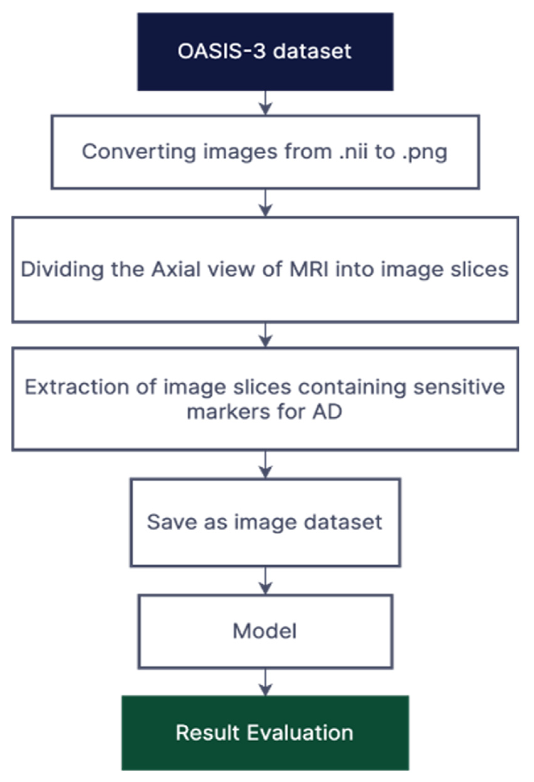
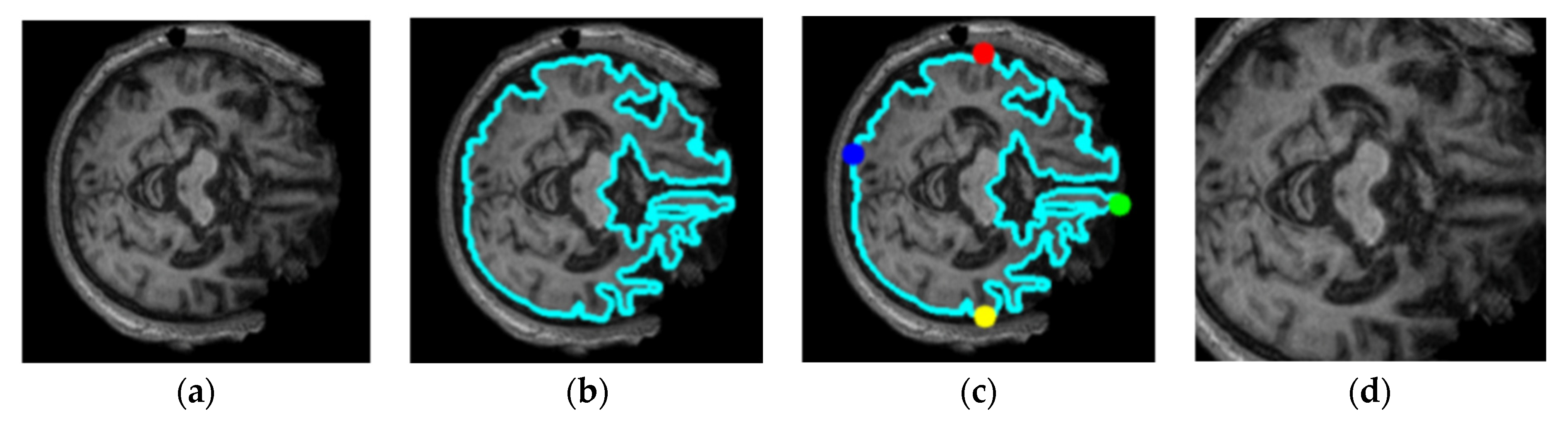
3.1. Dataset Pre-Processing

This experiment was performed on 113 subjects taken from OASIS-3: Longitudinal Multimodal Neuroimaging, Clinical, and Cognitive Dataset for Normal Aging and AD archive [46]. The MRI images are available in NifTI format. A total of 247 and 410 MRI scans were used for cognitively normal and mild cognitive impairment patients respectively. T1-weighted structural sequences were processed on the axial plane of brain MRIs. The Clinical Dementia Rating (CDR) Scale was used to determine the dataset’s dementia status; a score of 0 on the scale indicates cognitively normal, while a score of more than 0 but less than 2 indicates mild impairment. Each image in the dataset is completely characterised, and complete details are given.

The first task with this dataset was converting the image files from NifTI to PNG. Performing this conversion resulted in 255 slices of the axial view of the brain for each subject, as shown in Figure 1. Multiple axial scans of the brain of each patient were extracted, particularly the images containing the hippocampus embedded deep into the temporal lobe and some areas which demonstrate a significant shrinkage in some parts of the brain, were fed as an input to the neural network. Multiple slices of MRIs were extracted from each subject for accurate prediction of the disease. The middle slices contain more tissue than the border slices. Since tissues are a biomarker for dementia, central slices aid the system in precisely classifying disorders that resemble AD. For the categorisation of AD, the slices along the border are less helpful and more deceptive since they contain more of the bones and skulls. The central slices are therefore utilised for training. This section goes into great detail on the dataset preparation.

Figure 1. Illustration of the proposed methodology.

To make our predictions more robust, data augmentation technique was applied to our dataset. Since it is a classification model, the visual transformation mainly focused on flipping random images horizontally; rotating them by a certain degree and min-max normalisation; and rescaling inputs to the range of [0, 1], computed as follows:

$$y=\frac{(x-\min \left(x\right))}{(\max \left(x\right)-\min \left(x\right))},$$

(2)

where $\mathrm{m}\mathrm{i}\mathrm{n}\left(x\right)$ and $\mathrm{m}\mathrm{a}\mathrm{x}\left(x\right)$ are the minimum and maximum intensity values, respectively, for the entire dataset, and $y_i$ represents the normalised intensity value against location $x_i ($where $i\in [1,n]$). This helps our dataset to resolve the class imbalance issue, creating variations and generalizations for our model.

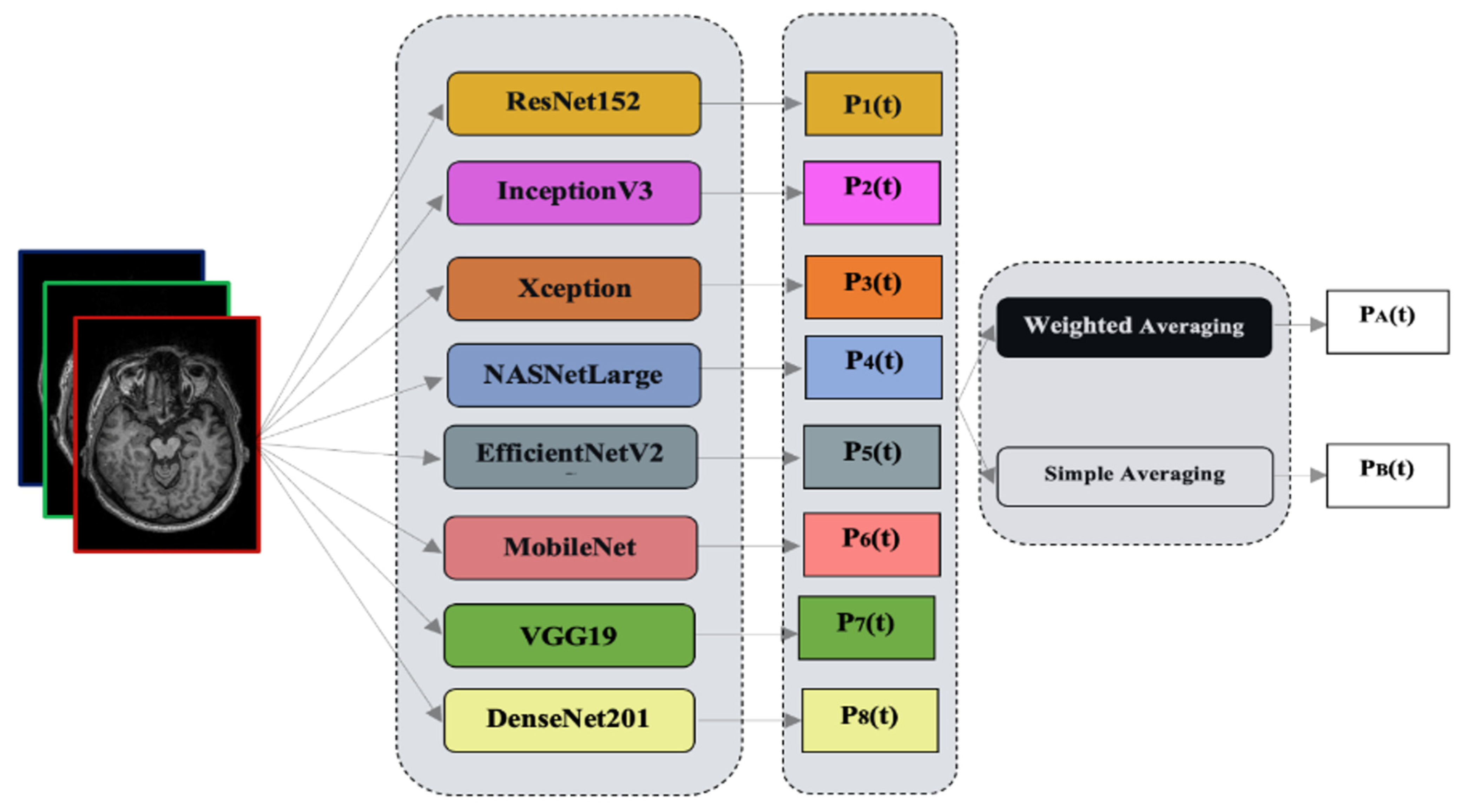
3.2. Ensemble Learning

Ensemble learning is a technique that combines the predictions of multiple individual models to make more accurate and robust predictions. It is widely used in machine learning and has shown promising results in various domains, including Alzheimer’s disease classification. In this paper, an ensemble of transfer learning models is proposed using two different methods: simple averaging and weighted averaging. By combining the predictions of these models, we aim to improve the extraction of sparse patterns and features from MRI images for Alzheimer’s disease diagnosis. These learning models are used for identifying Alzheimer’s disease. The proposed methodology’s block diagram is shown in Figure 2. Our transfer learning models are input with 2D image slices.

Figure 2. Graphical abstract of the proposed study.

Combining the judgements from several different models yields superior outcomes to those produced by a single model [47]. The generalization capacity of an ensemble, comprising multiple learners, is often considerably stronger than that of an individual learner, especially when it comes to weak learners. While an ensemble of weak learners can theoretically achieve good performance, in practice, people tend to prefer strong learners for various reasons. These reasons include minimizing the number of individual learners and leveraging the ability to reuse previously learned information about the strong learners [47].

In this paper, we utilise heterogeneous ensembles which have individual learners called component learners or simply individual learners. Unlike homogeneous ensembles, where all individual learners are of the same type, such as employing the same classification models, heterogeneous ensembles consist of diverse individual learners and learning algorithms, without relying on a single base learner or learning algorithm.

In order to compare and circumvent these problems, different ensemble models have been developed along with simple averaging. Weighted averaging provides various weights to various base learners. The goals were to determine which ensemble method had a strong correlation with the accuracy of the ensemble, which type of averaging had a high capacity to produce classification models that were not only accurate but also more diverse, and which types of ensembles were most likely to be able to enhance classification performance.

Simple Averaging: The most straightforward method to combine the output is by averaging them together. Let our ensemble contain $T$ individual learners $\{h_{1, }{h}_2,h_3,\dots \dots ,h_T\}$, where $h_i\left(x\right)$ is the result of $h_i$ on $x$ number of samples. The equation can be described as

$$H\left(x\right)=\frac{1}{T}{\sum }_{i=1}^T{h}_i\left(x\right),$$

(3)

This approach has the benefit being easily implemented [28], but it does not take into account that some models may perform better than others.

Weighted Averaging: The transfer learning model which has lower classification error is given a smaller weight when combined for ensembling, as described by [29]. The values of weights are assigned manually with the help of multiplying with a factor $\alpha$ to each model.

$$H\left(x\right)={\sum }_{i=1}^T{\alpha }_i{h}_i\left(x\right),$$

(4)

where $\alpha$ is the weight of an individual learner $h_i$, and ${\alpha }_i\ge 0$, ${\sum }_{i=1}^T{\alpha }_i=1$. It is shown in [30] that optimal choice for alpha is

$${\alpha }_{i=}\frac{\sum _j{C_{ij}}^{-1}}{\sum _k\sum _j{C_{kj}}^{-1}},$$

(5)

4. Experimentation and Results

4.1. Evaluation Indicators

The confusion matrix is a table that is commonly used in classification problems to evaluate the performance of a classification algorithm. It compares the actual and predicted values of a dataset and provides a summary of the number of true positives, true negatives, false positives, and false negatives for each class in a classification problem. The true positives (TP) are the number of correctly predicted positive instances, while the true negatives (TN) are the number of correctly predicted negative instances. The false positives (FP) are the number of negative instances that were incorrectly predicted as positive, and the false negatives (FN) are the number of positive instances that were incorrectly predicted as negative. Overall, the confusion matrix and its associated performance metrics provide valuable information for evaluating the performance of classification algorithms and identifying areas for improvement.

The following parameters and metrics are used for comparative analysis of data-driven models. In this study, the classifier correctly predicted TP and TN instances and incorrectly predicted FP and FN instances. The paper includes various performance metrics such as accuracy, sensitivity, specificity, and AUC score. It is a valuable tool for evaluating the performance of classification models and identifying areas where the model can be improved. To assess the unbiasing effectiveness of the proposed classification method, the TP, FP, FN, and TN statistical indices are computed and used to calculate accuracy, sensitivity, and specificity, as follows:

$$Accuracy=\frac{TP+FP}{TP+FP+TN+FN}$$

(6)

$$Sensitivity=\frac{TP}{TP+FN}$$

(7)

$$Specificity=\frac{TN}{TN+FP}$$

(8)

The entire dataset contained 657 images. The models are trained and evaluated using 5-fold cross-validation technique. We used 30 epochs with a batch size of 16. The learning rate was fixed at 0.001 for all architectures with the Adam optimizer.

4.2. Model Selection

This section evaluates different pre-trained deep convolutional networks [48,49,50,51,52,53,54,55] on the OASIS dataset, as shown in Table 1. It can be observed that the VGG19 model performed the best with an accuracy of 0.977, whereas NASNetLarge model scored the least with an accuracy of 0.912. MobileNet, DenseNet201, ResNet152, EfficientNetV2S, InceptionV3, and Xception scored an accuracy of 0.922, 0.961, 0.946, 0.952, 0.936, and 0.931, respectively. Furthermore, we improve the accuracy of the models using a cropping technique. The results demonstrate that DenseNet201 has a higher AUC score than VGG19, even though the accuracy of DenseNet201 is much less than that of VGG19. This discrepancy can be attributed to the fact that the AUC score only considers the ranking of the predicted probabilities. In contrast, the accuracy score considers both the ranking and the threshold for classification. In some cases, a model with a higher accuracy score may not have a better ROC curve and, thus, a lower AUC score.

Table 1. Performance of transfer learning models.

Models	Accuracy	Specificity	Sensitivity	AUC
MobileNet [48]	0.922	0.927	0.913	0.920
VGG19 [49]	0.977	0.949	0.961	0.958
DenseNet201 [50]	0.961	0.965	0.958	0.962
ResNet152 [51]	0.946	0.942	0.911	0.937
EfficientNetV2S [52]	0.952	0.966	0.943	0.959
InceptionV3 [53]	0.936	0.939	0.923	0.932
NASNetLarge [54]	0.912	0.927	0.913	0.920
Xception [55]	0.931	0.929	0.901	0.918

The cropping technique used extracted slices by finding the biggest contour, i.e., inside of the skull where the hippocampus is located. As shown in Figure 3, the extreme points of the brain were localised, which reduces the computation by exempting the pixels which do not contain the information of the features or unwanted space which may hinder the performance of classification model. The unwanted space also acts as noise for the image. To counter that, we applied threshold or canny edge detection, followed by finding the continuous points along the boundary having the same colour or intensity. The extreme points of the top, left, bottom, and right edges of the images were localised, and the same set of models with same hyperparameters as in without cropping the images were trained. As shown in Table 2, the performance of the eight models increased significantly in terms of accuracy and AUC score. It can be observed that VGG19 achieved the highest accuracy score of 0.982, and the lowest accuracy score was achieved by MobileNet. DenseNet201, ResNet152, EfficientNetV2S, InceptionV3, NASNetLarge, and Xception scored accuracies of 0.974, 0.966, 0.975, 0.952, 0.926, and 0.959, respectively. In terms of the AUC, VGG19 performed the best with a score of 0.986, whereas the lowest AUC score of 0.911 was achieved by NASNetLarge.

Figure 3. Illustration of the proposed cropping technique for the extracting region of interest: (a) original image, (b) finding the biggest contour, (c) finding the extreme points, (d) region of interest.

Table 2. Performance of transfer learning models using cropping technique.

Models	Accuracy	Specificity	Sensitivity	AUC
MobileNet [48]	0.915	0.892	0.867	0.899
VGG19 [49]	0.982	0.973	0.993	0.986
DenseNet201 [50]	0.974	0.967	0.975	0.969
ResNet152 [51]	0.966	0.957	0.968	0.959
EfficientNetV2S [52]	0.975	0.988	0.969	0.973
InceptionV3 [53]	0.952	0.947	0.962	0.942
NASNetLarge [54]	0.926	0.899	0.901	0.911
Xception [55]	0.959	0.944	0.966	0.954

4.3. Model Ensembling Strategy

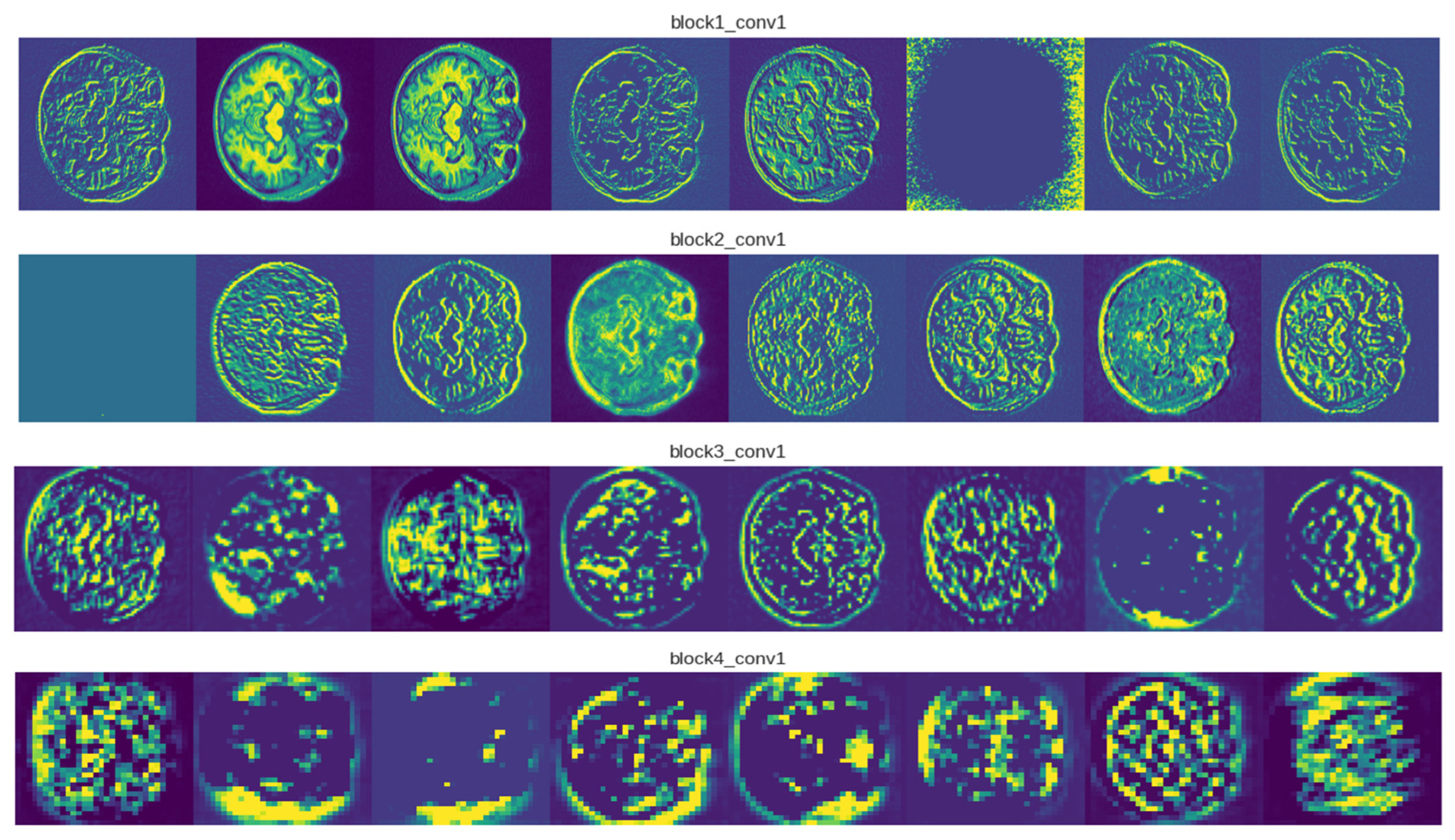
Training of these network was followed by ensembling in two ways i.e., simple averaging and weighted averaging. The experimentation settings for both the ensemble methods were kept same i.e., learning rate of 0.0001 with Adam optimizer and 100 Epochs. Images obtained through the cropping technique are used. Table 3 shows the performance of the two different ensemble methods. We select the best three models, i.e., VGG19, DenseNet201, and EfficientNetV2S according to Table 2 and denote their names as M1, M2, and M3 respectively. Next, we perform experiments by merging M1, M2, and M3 models in different combinations such as M1 + M2 + M3, M1 + M2, M2 + M3, and M1 + M3. According to Table 3, the best performance with an accuracy of 0.989 is achieved by combining models (M2 + M3) using simple averaging method. However, the lowest accuracy of 0.941 is achieved on M1 + M2 + M3 model that used weighted averaging method. In terms of the AUC, highest score is obtained by M1 + M2 with simple averaging method whereas lowest score is achieved by M1 + M2 + M3 model with weighted averaging method.

Table 3. Performance of ensemble networks using two different methods.

Ensemble Method	Models	Accuracy	Specificity	Sensitivity	AUC
Simple Average	M1 + M2 + M3	0.971	0.960	0.973	0.966
	M1 + M2	0.969	0.958	0.983	0.979
	M1 + M3	0.977	0.989	0.969	0.977
	M2 + M3	0.989	0.967	0.978	0.968
Weighted Average	M1 + M2 + M3	0.941	0.942	0.922	0.936
	M1 + M2	0.976	0.961	0.984	0.978
	M1 + M3	0.969	0.964	0.936	0.952
	M2 + M3	0.981	0.970	0.925	0.947

4.4. Visualizations

A feature map is produced as a result of the convolution operation being performed on the input by a convnet filter. To create an output volume, we apply a number of filters and stack the feature maps that are produced. Instead of looking at a single feature map, we have displayed multiple hidden feature maps in Figure 4 to show how the input is modified through subsequent layers. We exhibited eight VGG19 feature maps per layer for viewing purposes. As we move through different levels, there are several observations regarding the feature maps. Simple forms are picked up by the filters in the first layer. The hidden representation shows various cross-sectional anatomies of the brain, such as the hippocampus, cerebral artery, and different lobes. The majority of the information provided in the image is retained in the first layer feature maps, i.e., conv1 of block1. The first layers in CNN architectures typically serve as edge detectors. The feature maps appear to be an abstract depiction of the original when we delve deeper into the network. Despite being less visible to humans, they still encode useful features. As we dig deeper, the feature maps become sparser because the filters pick up fewer features.

Figure 4. Visualizations for examples of MRI images from the OASIS-3 dataset.

5. Conclusions

In this paper, we proposed an ensemble-based transfer learning approach using two methods: simple averaging and weighted averaging. The proposed framework extracts superior sparse patterns and features from MRI images. To avoid overfitting, we used data augmentation techniques. After obtaining superior results from experiments, it can be inferred that both ensemble methods are equally competent. Furthermore, we investigated the performance of the models using uncropped and cropped MRI images. In future work, we aim to further refine and expand the proposed ensemble framework by incorporating additional transfer learning models, exploring different ensembling approaches, evaluating its performance on various AD databases, and leveraging adversarial networks for synthetic image generation. We also plan to test the results of our architecture on other AD databases to improve the generalization of our model. These advancements can potentially enhance the accuracy, robustness, and generalization of the model for Alzheimer’s disease classification.

References

1. Alzheimer’s Association. 2022 Alzheimer’s Disease Facts and Figures. Alzheimer’s Dement. 2022, 18, 700–789. [Google Scholar] [CrossRef] [PubMed]
2. Thushara, A. An Efficient Alzheimer’s Disease Prediction Based on MEPC-SSC Segmentation and Momentum Geo-Transient MLPs. Comput. Biol. Med. 2022, 151, 106247. [Google Scholar] [CrossRef] [PubMed]
3. Thapa, S.; Singh, P.; Jain, D.K.; Bharill, N.; Gupta, A.; Prasad, M. Data-Driven Approach Based on Feature Selection Technique for Early Diagnosis of Alzheimer’s Disease. In Proceedings of the 2020 International Joint Conference on Neural Networks (IJCNN), Glasgow, UK, 19–24 July 2020; pp. 1–8. [Google Scholar]
4. Adhikari, S.; Thapa, S.; Naseem, U.; Singh, P.; Huo, H.; Bharathy, G.; Prasad, M. Exploiting Linguistic Information from Nepali Transcripts for Early Detection of Alzheimer’s Disease Using Natural Language Processing and Machine Learning Techniques. Int. J. Hum. Comput. Stud. 2022, 160, 102761. [Google Scholar] [CrossRef]
5. Tanveer, M.; Richhariya, B.; Khan, R.U.; Rashid, A.H.; Khanna, P.; Prasad, M.; Lin, C.T. Machine Learning Techniques for the Diagnosis of Alzheimer’s Disease. ACM Trans. Multimed. Comput. Commun. Appl. 2020, 16, 1–35. [Google Scholar] [CrossRef]
6. Tremblay-Mercier, J.; Madjar, C.; Das, S.; Pichet Binette, A.; Dyke, S.O.M.; Étienne, P.; Lafaille-Magnan, M.-E.; Remz, J.; Bellec, P.; Louis Collins, D.; et al. Open Science Datasets from PREVENT-AD, a Longitudinal Cohort of Pre-Symptomatic Alzheimer’s Disease. NeuroImage Clin. 2021, 31, 102733. [Google Scholar] [CrossRef] [PubMed]
7. Poulin, S.P.; Dautoff, R.; Morris, J.C.; Barrett, L.F.; Dickerson, B.C. Amygdala Atrophy Is Prominent in Early Alzheimer’s Disease and Relates to Symptom Severity. Psychiatry Res. Neuroimaging 2011, 194, 7–13. [Google Scholar] [CrossRef] [PubMed]
8. Westman, E.; Cavallin, L.; Muehlboeck, J.-S.; Zhang, Y.; Mecocci, P.; Vellas, B.; Tsolaki, M.; Kłoszewska, I.; Soininen, H.; Spenger, C.; et al. Sensitivity and Specificity of Medial Temporal Lobe Visual Ratings and Multivariate Regional MRI Classification in Alzheimer’s Disease. PLoS ONE 2011, 6, e22506. [Google Scholar] [CrossRef]
9. Gupta, A.; Kumar, D.; Verma, H.; Tanveer, M.; Javier, A.P.; Lin, C.-T.; Prasad, M. Recognition of Multi-Cognitive Tasks from EEG Signals Using EMD Methods. Neural Comput. Appl. 2022. [Google Scholar] [CrossRef]
10. Kiani, M.; Andreu-Perez, J.; Hagras, H.; Papageorgiou, E.I.; Prasad, M.; Lin, C.-T. Effective Brain Connectivity for FNIRS With Fuzzy Cognitive Maps in Neuroergonomics. IEEE Trans. Cogn. Dev. Syst. 2022, 14, 50–63. [Google Scholar] [CrossRef]
11. Ding, W.; Lin, C.-T.; Prasad, M. Hierarchical Co-Evolutionary Clustering Tree-Based Rough Feature Game Equilibrium Selection and Its Application in Neonatal Cerebral Cortex MRI. Expert Syst. Appl. 2018, 101, 243–257. [Google Scholar] [CrossRef]
12. Lazli, L.; Boukadoum, M.; Mohamed, O.A. A Survey on Computer-Aided Diagnosis of Brain Disorders through MRI Based on Machine Learning and Data Mining Methodologies with an Emphasis on Alzheimer Disease Diagnosis and the Contribution of the Multimodal Fusion. Appl. Sci. 2020, 10, 1894. [Google Scholar] [CrossRef]
13. Chen, Z.S.; Kulkarni, P.; Galatzer-Levy, I.R.; Bigio, B.; Nasca, C.; Zhang, Y. Modern Views of Machine Learning for Precision Psychiatry. Patterns 2022, 3, 100602. [Google Scholar] [CrossRef] [PubMed]
14. Zhang, Y.; Zhang, H.; Adeli, E.; Chen, X.; Liu, M.; Shen, D. Multiview Feature Learning With Multiatlas-Based Functional Connectivity Networks for MCI Diagnosis. IEEE Trans. Cybern. 2022, 52, 6822–6833. [Google Scholar] [CrossRef]
15. Anh, N.; Prasad, M.; Srikanth, N.; Sundaram, S. Wave Forecasting Using Meta-Cognitive Interval Type-2 Fuzzy Inference System. Procedia Comput. Sci. 2018, 144, 33–41. [Google Scholar] [CrossRef]
16. Za’in, C.; Pratama, M.; Prasad, M.; Puthal, D.; Lim, C.P.; Seera, M. Motor Fault Detection and Diagnosis Based on a Meta-Cognitive Random Vector Functional Link Network. In Fault Diagnosis of Hybrid Dynamic and Complex Systems; Springer International Publishing: Cham, Switzerland, 2018; pp. 15–44. [Google Scholar]
17. Castellazzi, G.; Cuzzoni, M.G.; Cotta Ramusino, M.; Martinelli, D.; Denaro, F.; Ricciardi, A.; Vitali, P.; Anzalone, N.; Bernini, S.; Palesi, F.; et al. A Machine Learning Approach for the Differential Diagnosis of Alzheimer and Vascular Dementia Fed by MRI Selected Features. Front. Neuroinform. 2020, 14. [Google Scholar] [CrossRef] [PubMed]
18. Battineni, G.; Chintalapudi, N.; Amenta, F.; Traini, E. A Comprehensive Machine-Learning Model Applied to Magnetic Resonance Imaging (MRI) to Predict Alzheimer’s Disease (AD) in Older Subjects. J. Clin. Med. 2020, 9, 2146. [Google Scholar] [CrossRef] [PubMed]
19. Alickovic, E.; Subasi, A. Automatic Detection of Alzheimer Disease Based on Histogram and Random Forest; Springer: Berlin/Heidelberg, Germany, 2020; pp. 91–96. [Google Scholar]
20. Bandyopadhyay, A.; Ghosh, S.; Bose, M.; Singh, A.; Othmani, A.; Santosh, K. Alzheimer’s Disease Detection Using Ensemble Learning and Artificial Neural Networks; Springer: Berlin/Heidelberg, Germany, 2023; pp. 12–21. [Google Scholar]
21. Wang, H.; Shen, Y.; Wang, S.; Xiao, T.; Deng, L.; Wang, X.; Zhao, X. Ensemble of 3D Densely Connected Convolutional Network for Diagnosis of Mild Cognitive Impairment and Alzheimer’s Disease. Neurocomputing 2019, 333, 145–156. [Google Scholar] [CrossRef]
22. Ortiz, A.; Munilla, J.; Górriz, J.M.; Ramírez, J. Ensembles of Deep Learning Architectures for the Early Diagnosis of the Alzheimer’s Disease. Int. J. Neural Syst. 2016, 26, 1650025. [Google Scholar] [CrossRef]
23. Tanveer, M.; Rashid, A.H.; Ganaie, M.A.; Reza, M.; Razzak, I.; Hua, K.-L. Classification of Alzheimer’s Disease Using Ensemble of Deep Neural Networks Trained Through Transfer Learning. IEEE J. Biomed. Health Inform. 2022, 26, 1453–1463. [Google Scholar] [CrossRef]
24. Girshick, R.; Donahue, J.; Darrell, T.; Malik, J. Rich Feature Hierarchies for Accurate Object Detection and Semantic Segmentation. arXiv 2013, arXiv:1311.2524. [Google Scholar]
25. Yosinski, J.; Clune, J.; Bengio, Y.; Lipson, H. How Transferable Are Features in Deep Neural Networks? arXiv 2014, arXiv:1411.1792. [Google Scholar]
26. Balaji, P.; Chaurasia, M.A.; Bilfaqih, S.M.; Muniasamy, A.; Alsid, L.E.G. Hybridized Deep Learning Approach for Detecting Alzheimer’s Disease. Biomedicines 2023, 11, 149. [Google Scholar] [CrossRef] [PubMed]
27. Pei, Z.; Wan, Z.; Zhang, Y.; Wang, M.; Leng, C.; Yang, Y.-H. Multi-Scale Attention-Based Pseudo-3D Convolution Neural Network for Alzheimer’s Disease Diagnosis Using Structural MRI. Pattern Recognit. 2022, 131, 108825. [Google Scholar] [CrossRef]
28. Liu, M.; Cheng, D.; Wang, K.; Wang, Y. Multi-Modality Cascaded Convolutional Neural Networks for Alzheimer’s Disease Diagnosis. Neuroinformatics 2018, 16, 295–308. [Google Scholar] [CrossRef] [PubMed]
29. Abdou, M.A. Literature Review: Efficient Deep Neural Networks Techniques for Medical Image Analysis. Neural Comput. Appl. 2022, 34, 5791–5812. [Google Scholar] [CrossRef]
30. Zhang, T.; Shi, M. Multi-Modal Neuroimaging Feature Fusion for Diagnosis of Alzheimer’s Disease. J. Neurosci. Methods 2020, 341, 108795. [Google Scholar] [CrossRef]
31. Odusami, M.; Maskeliūnas, R.; Damaševičius, R.; Misra, S. Explainable Deep-Learning-Based Diagnosis of Alzheimer’s Disease Using Multimodal Input Fusion of PET and MRI Images. J. Med. Biol. Eng. 2023, 43, 291–302. [Google Scholar] [CrossRef]
32. Yu, W.; Lei, B.; Ng, M.K.; Cheung, A.C.; Shen, Y.; Wang, S. Tensorizing GAN With High-Order Pooling for Alzheimer’s Disease Assessment. IEEE Trans. Neural Netw. Learn. Syst. 2022, 33, 4945–4959. [Google Scholar] [CrossRef]
33. Shi, J.; Zheng, X.; Li, Y.; Zhang, Q.; Ying, S. Multimodal Neuroimaging Feature Learning With Multimodal Stacked Deep Polynomial Networks for Diagnosis of Alzheimer’s Disease. IEEE J. Biomed. Health Inform. 2018, 22, 173–183. [Google Scholar] [CrossRef]
34. Zhang, X.; Yao, L.; Wang, X.; Monaghan, J.; McAlpine, D.; Zhang, Y. A Survey on Deep Learning-Based Non-Invasive Brain Signals: Recent Advances and New Frontiers. J. Neural Eng. 2021, 18, 031002. [Google Scholar] [CrossRef]
35. Suk, H.-I.; Lee, S.-W.; Shen, D. Deep Ensemble Learning of Sparse Regression Models for Brain Disease Diagnosis. Med. Image Anal. 2017, 37, 101–113. [Google Scholar] [CrossRef] [PubMed]
36. Feng, W.; Van Halm-Lutterodt, N.; Tang, H.; Mecum, A.; Mesregah, M.K.; Ma, Y.; Li, H.; Zhang, F.; Wu, Z.; Yao, E.; et al. Automated MRI-Based Deep Learning Model for Detection of Alzheimer’s Disease Process. Int. J. Neural Syst. 2020, 30, 2050032. [Google Scholar] [CrossRef] [PubMed]
37. Wang, S.; Wang, H.; Shen, Y.; Wang, X. Automatic Recognition of Mild Cognitive Impairment and Alzheimers Disease Using Ensemble Based 3D Densely Connected Convolutional Networks. In Proceedings of the 2018 17th IEEE International Conference on Machine Learning and Applications (ICMLA), Orlando, FL, USA, 17–20 December 2018; pp. 517–523. [Google Scholar]
38. Jain, R.; Jain, N.; Aggarwal, A.; Hemanth, D.J. Convolutional Neural Network Based Alzheimer’s Disease Classification from Magnetic Resonance Brain Images. Cogn. Syst. Res. 2019, 57, 147–159. [Google Scholar] [CrossRef]
39. Zhu, W.; Sun, L.; Huang, J.; Han, L.; Zhang, D. Dual Attention Multi-Instance Deep Learning for Alzheimer’s Disease Diagnosis With Structural MRI. IEEE Trans. Med. Imaging 2021, 40, 2354–2366. [Google Scholar] [CrossRef]
40. Chen, Y.; Shi, B.; Wang, Z.; Zhang, P.; Smith, C.D.; Liu, J. Hippocampus Segmentation through Multi-View Ensemble ConvNets. In Proceedings of the 2017 IEEE 14th International Symposium on Biomedical Imaging (ISBI 2017), Melbourne, Australia, 18–21 April 2017; pp. 192–196. [Google Scholar]
41. Ataloglou, D.; Dimou, A.; Zarpalas, D.; Daras, P. Fast and Precise Hippocampus Segmentation Through Deep Convolutional Neural Network Ensembles and Transfer Learning. Neuroinformatics 2019, 17, 563–582. [Google Scholar] [CrossRef]
42. Zhang, D.; Shen, D. Semi-Supervised Multimodal Classification of Alzheimer’s Disease. In Proceedings of the 2011 IEEE International Symposium on Biomedical Imaging: From Nano to Macro, Chicago, IL, USA, 30 March–2 April 2011; pp. 1628–1631. [Google Scholar]
43. Liu, S.; Liu, S.; Cai, W.; Che, H.; Pujol, S.; Kikinis, R.; Feng, D.; Fulham, M.J. ADNI Multimodal Neuroimaging Feature Learning for Multiclass Diagnosis of Alzheimer’s Disease. IEEE Trans. Biomed. Eng. 2015, 62, 1132–1140. [Google Scholar] [CrossRef]
44. Liu, C.; Huang, F.; Qiu, A. Monte Carlo Ensemble Neural Network for the Diagnosis of Alzheimer’s Disease. Neural Netw. 2023, 159, 14–24. [Google Scholar] [CrossRef] [PubMed]
45. Yang, Y.; Li, X.; Wang, P.; Xia, Y.; Ye, Q. Multi-Source Transfer Learning via Ensemble Approach for Initial Diagnosis of Alzheimer’s Disease. IEEE J. Transl. Eng. Health Med. 2020, 8, 1–10. [Google Scholar] [CrossRef]
46. LaMontagne, P.J.; Benzinger, T.L.S.; Morris, J.C.; Keefe, S.; Hornbeck, R.; Xiong, C.; Grant, E.; Hassenstab, J.; Moulder, K.; Vlassenko, A.G.; et al. OASIS-3: Longitudinal Neuroimaging, Clinical, and Cognitive Dataset for Normal Aging and Alzheimer Disease. medRxiv 2019. [Google Scholar] [CrossRef]
47. Ganaie, M.A.; Hu, M.; Malik, A.K.; Tanveer, M.; Suganthan, P.N. Ensemble Deep Learning: A Review. Eng. Appl. Artif. Intell. 2022, 115, 105151. [Google Scholar] [CrossRef]
48. Howard, A.G.; Zhu, M.; Chen, B.; Kalenichenko, D.; Wang, W.; Weyand, T.; Andreetto, M.; Adam, H. MobileNets: Efficient Convolutional Neural Networks for Mobile Vision Applications. arXiv 2017, arXiv:1704.04861. [Google Scholar]
49. Simonyan, K.; Zisserman, A. Very Deep Convolutional Networks for Large-Scale Image Recognition. arXiv 2014, arXiv:1409.1556. [Google Scholar]
50. Huang, G.; Liu, Z.; van der Maaten, L.; Weinberger, K.Q. Densely Connected Convolutional Networks. arXiv 2016, arXiv:1608.06993. [Google Scholar]
51. He, K.; Zhang, X.; Ren, S.; Sun, J. Deep Residual Learning for Image Recognition. arXiv 2015, arXiv:1512.03385. [Google Scholar]
52. Tan, M.; Le, Q.V. EfficientNetV2: Smaller Models and Faster Training. arXiv 2021, arXiv:2104.00298. [Google Scholar]
53. Szegedy, C.; Vanhoucke, V.; Ioffe, S.; Shlens, J.; Wojna, Z. Rethinking the Inception Architecture for Computer Vision. arXiv 2015, arXiv:1512.00567. [Google Scholar]
54. Zoph, B.; Vasudevan, V.; Shlens, J.; Le, Q.V. Learning Transferable Architectures for Scalable Image Recognition. arXiv 2017, arXiv:1707.07012. [Google Scholar]
55. Chollet, F. Xception: Deep Learning with Depthwise Separable Convolutions. arXiv 2016, arXiv:1610.02357. [Google Scholar]
Disclaimer/Publisher’s Note: The statements, opinions and data contained in all publications are solely those of the individual author(s) and contributor(s) and not of MDPI and/or the editor(s). MDPI and/or the editor(s) disclaim responsibility for any injury to people or property resulting from any ideas, methods, instructions or products referred to in the content.
Article Metrics
Citations
Article Access Statistics
Multiple requests from the same IP address are counted as one view.