Abstract
Bayesian neural networks (BNNs) are effective tools for a variety of tasks that allow for the estimation of the uncertainty of the model. As BNNs use prior constraints on parameters, they are better regularized and less prone to overfitting, which is a serious issue for brain–computer interfaces (BCIs), where typically only small training datasets are available. Here, we tested, on the BCI Competition IV 2a motor imagery dataset, if the performance of the widely used, effective neural network classifiers EEGNet and Shallow ConvNet can be improved by turning them into BNNs. Accuracy indeed was higher, at least for a BNN based on Shallow ConvNet with two of three tested prior distributions. We also assessed if BNN-based uncertainty estimation could be used as a tool for out-of-domain (OOD) data detection. The OOD detection worked well only in certain participants; however, we expect that further development of the method may make it work sufficiently well for practical applications.
1. Introduction
In brain–computer interface (BCI) classification problems, only a small dataset is typically available for classifier training, which leads to suboptimal classifier performance [1]. Neural network classifiers, which in the last decade revolutionized many machine learning applications, are especially prone to this problem. It is, therefore, highly desirable that the classifiers used in BCIs could be well-trained on small datasets.
Moreover, due to the small train dataset size and also because the user’s or participant’s brain state may significantly change between classifier calibration and application time periods, the classifier may meet some patterns in the brain signal unseen during its training. In such cases, the classifier has to choose from a limited number of classes it has been trained on despite the fact that it has never seen such a pattern before. Obviously, this leads to mistakes and a decrease in the classification quality. Other sources of patterns unseen in training are brain signal variability and non-stationarity [2], which can be especially strong due to the user’s/participant’s fatigue, distraction, or stress but also due to normal variations in the brain state. To avoid such mistakes, BCI algorithms should be able to recognize the unseen patterns as unseen and not try to report them as belonging to one of the known classes. This can be achieved using the out-of-domain (OOD) data detection approaches. One can define the out of domain input vector as a vector that semantically differs from a training set but is present in the testing set. The OOD data detection issue is relevant in many areas, especially in the sphere of the NLP. There were numerous methods addressing this issue [3,4], even quite sophisticated ones, using generative adversarial networks [5]. The OOD detection was found relevant and effective in the sphere of medicine [6] and robotics [7]; the OOD detection methods were even applied to the problems of particle physics [8]. The amount of methods addressing the OOD detection problem continues to flourish. Solid baselines regarding different areas of science were established, such as stochastic weight averaging [9] or calibration of softmax prediction probability values [10]. Given all the mentioned applications in other areas, it is surprising that OOD detection has been so far very little explored for BCIs. A related problem, uncertainty estimation, was addressed in two BCI studies regarding the uncertainty reduction [11] and classification with rejection option [12] problems but without application for the OOD detection.
Both the problem of enabling the training of the classifiers on small datasets and the OOD problem can be addressed using Bayesian neural networks (BNN). BNNs encode prior assumptions about the desired behavior of the classification model. They form a well-known class of algorithms [13]. The key difference between Bayesian and deterministic neural networks is that the weights are considered stochastic variables, with an arbitrarily chosen prior distribution before the data is seen. The goal is to find a posterior distribution after data observation. It can be found using the Bayes’ theorem [14]:
where w and D represent the parameters of the BNN and the dataset, respectively; hence, the learning problem, which equals the optimization problem for deterministic neural networks, becomes a Bayesian inference problem in application to BNNs. The denominator on the right side of (1) can be rewritten in this form:
As can be seen from (2), there is a need to integrate all the space of the parameters in the model, which is a high-dimensional one. Thus, in a majority of cases, the exact inference is intractable, so that the approximations, such as variational inference or sampling methods, are used.
The main feature of the BNNs is prior constraints for the parameters, which leads to better regularization of the loss function, i.e., stricter restrictions on weights. More information on this matter was provided by Jospin et al. [13] and Wang and Yeung [15]. Hence, BNNs are less prone to overfitting, a great advantage for a neural network when training datasets are small. Because of this improvement, the BNN may have better generalization properties.
BNNs have been used in BCI for years, and in a few recent papers, they were successfully applied to enhance the performance of some existing deterministic neural networks for various types of data and experimental paradigms, such as EEG under motor imagery [12], the P300 potential [16], fNIRS data [17]. However, of special interest could be similar to the “Bayesian” enhancement of the most widely used, effective, and well-studied architectures, which we undertook in this study.
Because of the BNN’s ability to quantify the uncertainty of its predictions, we expect that the BNN-based OOD detection methods can also address the issue of OOD data in BCIs. The BNNs can be considered as an ensemble of an infinite number of neural networks [18]. Since the ensembles can provide one with an uncertainty metric [19], such as entropy [20] or variance of predictions across all of its nets, there is a perspective to use this type of algorithm for discovering OOD data. During BCI classifier application, including practical real-time scenarios, the BCI can be made to refrain from issuing a command when OOD is detected. The ability of BNNs to provide high-quality OOD detection was doubted by Henning et al. [21]. However, they studied data with fewer dimensions than is typical for the EEG.
In this paper, we:
- Assess performance enhancement in an EEG-based BCI task when two widely used deterministic neural network classifiers, EEGNet [22] and Shallow ConvNet [23], were turned into BNNs.
- Assess the ability of these BNNs to enable OOD detection.
2. Materials and Methods
2.1. Dataset
The dataset used in this paper is an open dataset, BCI Competition IV 2a [24]. It is an EEG motor imagery dataset consisting of 9 participants, with 576 trials per participant. Each participant had two experimental sessions, T and E, 288 trials each. These two sessions were used to form train and test sets, respectively. There are four classes of movements, imaged by participants, marked with numbers from 0 to 3, with respect to the body parts of motor imaging, namely: left hand, right hand, feet, and tongue. The EEG data was recorded using 22 channels and with a 250 Hz frequency. Each trial was six seconds long. In the last three seconds, the motor imagery was performed. The data was bandpass-filtered between 4 Hz and 38 Hz, followed by extraction of trials from the recording. Although informative features could likely occupy a narrow frequency range, being related to mu- and beta-rhythms, we opted for this frequency range in order to be consistent with Schirrmeister et al. [23]. In our view, using their parameters makes sense because a narrower frequency range is not always an optimal solution because the features of interest could have a wider spectrum than the standard definition of a rhythm’s band; moreover, the network should fit a filter for separating the informative components from the non-informative ones, and they also can surpass the predefined bounds. Finally, features that are informative for OOD data detection are not necessarily the same that are useful for movement imagery detection. After preprocessing, each trial could be presented as a matrix sized 22 × 1125.
To model the presence of the out-of-domain data, the training set was modified as follows. From the training set, we deleted two classes of trials, labeled as “feet” and “tongue”, leaving another two classes, “left hand” and “right hand”. We decided to split the dataset in this way, considering the similar nature of the EEG signals related to left and right hands compared to the other types of motor imagination. Thus, the modified training set consisted of two classes and 144 trials per participant, whereas the test dataset has not undergone any changes. Therefore, we could treat the two classes used for training as “in-domain” data and the two classes not used for training as “out-of-domain” data.
2.2. Architectures and Related Methods
In this study, the wide-spread deterministic architectures were used: EEGNetV4 [22] and Shallow ConvNet [23], with hyperparameters, such as dropout, defined in the respective papers. These architectures were converted to Bayesian algorithms by imposing prior distribution over the weights. In other words, we assumed that each weight of the network is a stochastic variable. Its probability distribution a priori is defined explicitly. Our goal was to obtain a posterior distribution of each parameter after observing the training data; for neural networks, the posterior distribution is intractable. It is possible to obtain samples from the posterior distribution using various Markov Chain Monte Carlo (MCMC) techniques. These methods construct a Markov chain of weight samples that converges to a posterior distribution of model weights. Until recently, Markov Chain Monte Carlo (MCMC) methods were widely used in Bayesian inference due to their ability to approximate complex posterior distributions. However, their drawback was the requirement for a large number of iterations to achieve convergence, which made them computationally expensive and time-consuming. Additionally, MCMC methods needed to evaluate the likelihood function over the entire batch of data at each iteration, which further added to the computational burden, especially for large datasets.
To address these limitations, Variational Inference (VI) techniques gained popularity within the Bayesian community. VI offered a faster alternative by approximating the posterior distribution with a more tractable family of parameterized distributions. This approach made it computationally efficient and enabled quicker convergence. Nonetheless, a major concern with VI was that it only provided samples from an approximate posterior, potentially leading to biased estimates compared to the true posterior distribution. Furthermore, VI required selecting an appropriate approximation family, such as Gaussian distributions, which might not capture the complexities of the true posterior distribution accurately. This choice of approximation family often necessitated intensive tuning efforts and expertise, making it less approachable for less experienced practitioners.
Fortunately, recent advancements in the field of Bayesian machine learning introduced a new family of stochastic gradient MCMC techniques. These methods cleverly combine the strengths of both MCMC and stochastic gradient optimization, allowing for efficient sampling from the true posterior distribution at significantly reduced computational costs.
By leveraging the idea of stochastic gradients, these new techniques achieve faster convergence by using mini-batches of data instead of evaluating the likelihood function over the entire dataset. This results in a dramatic reduction in computational time while still providing high-quality posterior samples.
Moreover, unlike Variational Inference, these stochastic gradient MCMC methods generate samples directly from the true posterior distribution, thereby eliminating any potential bias introduced by approximation. This crucial advantage has made them increasingly popular for Bayesian inference tasks, as they can provide more accurate uncertainty estimates and improved predictions.
Modern MCMC methods utilize the gradient of the log-likelihood function, equivalent to the loss function of deterministic models. For users, the process is similar to standard optimization of a neural network’s loss function, with a log-likelihood replacing the loss function, a log-prior probability density replacing the weight’s regularization constraint, and an MCMC sampler replacing the optimizer. The main difference is the need to collect multiple weight samples after the Markov chain converges instead of a single set of weights in standard optimization.
To obtain predictions of BNN, we used the Monte Carlo approach. For this purpose, we collected 120 weight samples from the posterior distribution and used them to construct an ensemble of 120 networks.
We used a set of prior distributions proposed by Fortuin et al. [25].
A standard isotropic Gaussian (IG) for all layers was considered as a basic approach. In order to increase the accuracy of classification, we used a standard IQ for all layers except the last, the fully connected one. For the latter, we opted for the Student-t distribution with N-1 degrees of freedom (where N is the number of weights in the classification layer), specifically with σ = 1.0 and mean μ = 0.0. Then we tried a combination of Correlated Gaussian (CG) with Matern kernel, IG, and t-distribution: CG was used in layers with spatial and temporal convolutions, t-distribution (σ = 1.0, μ = 0.0) was used in fully connected layer, and IG was used in EEGNet architecture for separable and pointwise convolutions. The CG was used in order to capture spatial and temporal correlations of the EEG data. The entries of the spatial correlation matrix were proportional to the distance between respective electrodes, whereas the entries of the temporal one were proportional to the relative time distance.
For the inference of the posterior of BNNs, the modification of SGHMC, called AdaptiveSGHMC [26], is used as a sampling technique.
We used ensembles of deterministic models of each considered architecture with 120 instances as a baseline. For deterministic nets, we used the AdamW algorithm [27].
We evaluated the out-of-domain detection performance using the ROC-AUC metric of the naive classifier. The predictor variable was the variance of pre-softmax activations of the model, and the binary response variable was whether the sample belonged to the in-domain or out-of-domain category. For assessing the measure of generalization properties of considered models BNNs, we use the classification accuracy metric.
The code of the numerical experiments was written in Python and PyTorch [28]. We used the Braindecode [23,29] package to preprocess the EEG data. The graphs and charts were plotted using Matplotlib [30] and Seaborn [31] libraries for Python. Statistical tests were conducted using the scipy [32] package.
The experiments were conducted using the CPU Intel® Core™ i5-4460 and GPU Gigabyte™ NVIDIA® GeForce RTX™ 3060.
2.3. Experiments
To evaluate the benefits of the Bayesian approach to the BCI problem, we performed two sets of experiments. The first set was intended to check if BNNs can improve the generalization properties of neural networks commonly used in BCIs. The second set of experiments is intended to investigate the capability of BNNs to detect out-of-domain input data.
For the experiments on the generalization properties of BNNs, we used the following procedure. For BNNs, we sampled four chains of weight samples, 40 samples each. In each chain, we discarded the first ten samples so that 120 weight samples in total were obtained. The burn-in phase consisted of 200 steps. The sampler was run with step length equal to 0.01 and momentum decay equal to 0.01. Each 200th sample was saved to make predictions on a test set. These values were suggested by Tran [33] for experiments on low-dimensional data.
Deterministic, i.e., non-Bayesian versions of the same models, were used as a baseline. These models were trained on 350 epochs for EEGNet and 100 epochs for Shallow ConvNet. For both deterministic nets and their ensembles, we used the learning rate of 0.000625 and set the momentum decay value to zero, as recommended in Braindecode tutorials.
The batch size was 288 and 64 for Bayesian and deterministic networks, respectively. The final prediction was an average across predictions of all samples or instances of the ensemble.
The values of all hyperparameters are presented in Table 1.

Table 1.
List of hyperparameters used for BNN and ensembles of deterministic neural networks. n/a stands for “not applicable”.
This experiment was conducted using all four classes of data and the BNNs of the same architectures with the settings specified above. The deterministic network architectures used in this experiment were single EEGNet and Shallow ConvNet networks using the settings mentioned above. These networks were fitted using the whole BCI competition IV 2a dataset without the exclusion of any classes.
In the OOD detection experiments, we maintained consistency with the first series of experiments by using the same inference and optimization procedures. This included using the same hyperparameter values, number of training and Bayesian inference epochs, and procedure of collecting weight samples from the posterior distribution. As was mentioned above, we used only 2 classes in training data: left and right-hand imaginary movement. We used ensembles of considered model architectures as a baseline in this experiment. Each ensemble contained 120 instances of deterministic models. The out-of-domain detection method for EEG data presented here is as follows. As the measure of uncertainty, the variance across the logits estimated by all samples or ensemble elements was used. Because the logit vector had 2 dimensions, we calculated its Euclidean norm to obtain a single value. The variance of BNN and ensemble predictions was collected on each data point in the test set. Then, the obtained variance was compared with a threshold: if the variance was greater, then the data point under consideration was labeled as “out of domain”, else it was marked as “in domain”. We used a set of thresholds from −1.0 to 1.0 with step 0.005. The method was evaluated on the test set, and for each threshold, the true-positive and false-positive rates were obtained. These rates were utilized to plot the ROC curve.
Data division into train and test sets was described above in the Dataset section.
The flowcharts of the OOD detector and experiments are presented in Figure 1, Figure 2 and Figure 3.
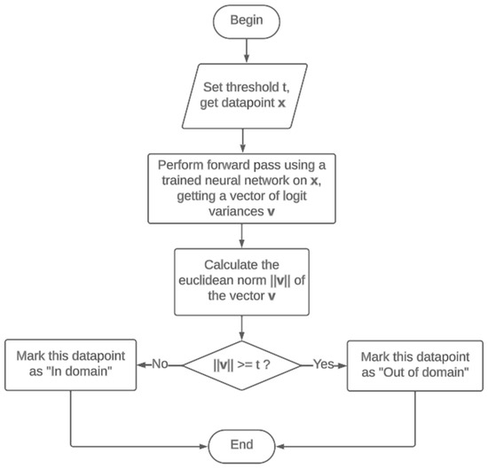
Figure 1.
Flowchart of the OOD data detector.
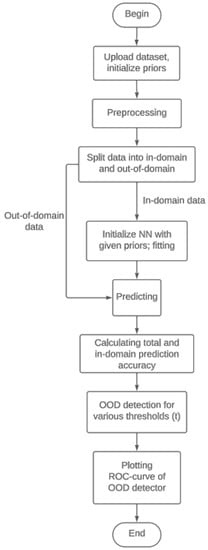
Figure 2.
Flowchart of the OOD data detection experiment.
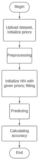
Figure 3.
Flowchart of measuring the accuracy.
3. Results
3.1. Accuracy of in-Domain Data Classification
The accuracy of BNNs under various prior constraints proved to be higher compared to their deterministic ensemble counterparts for both architectures. This can be stated for most of the participants (Figure 4 and Figure 5) for both architectures. These differences proved to be statistically insignificant for EEGNet architecture (Ensemble vs. IG: T = 10.5, p = 0.16, IG vs. IG + t: T = 15.0, p = 0.67, IG vs. CG + t: T = 16.5, p = 0.57), though, which is shown by Wilcoxon signed rank test. However, for Shallow ConvNet architecture, there are some statistical differences, shown by the Wilcoxon signed rank test (Ensemble vs. IG: T = 5.5, p = 0.04, IG vs. IG + t: T = 3.5, p = 0.07, IG vs. CG + t: T = 2.0, p = 0.01). Group average data are shown for EEGNet and Shallow ConvNet in Figure 6 and Figure 7, respectively; noticeably, Shallow ConvNet accuracy seems to increase with prior complexity.
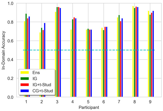
Figure 4.
Values of In-Domain 2-classes accuracy for all participants, using different prior constraints compared to the ensemble for EEGNet architecture. Ens stands for ‘Ensemble of 120 deterministic models’, IG stands for Isotropic Gaussian prior for all layers, IG + t-Stud stands for IG for all layers and t-Student prior for the classification layer, CG + t-Stud stands for Correlated Gaussian prior for temporal and spatial convolution layers, t-Student prior for the classification layer and IG for all other layers. The cyan dashed line represents the 0.5 threshold of random guessing.
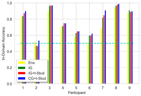
Figure 5.
Values of In-Domain 2-classes accuracy for all participants, using different prior constraints compared to the ensemble for Shallow ConvNet architecture. The cyan dashed line represents the 0.5 threshold of random guessing. See Figure 3 caption for other details.
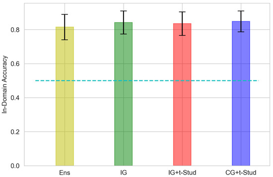
Figure 6.
Values of In-Domain 2-classes accuracy averaged across all participants, using different prior constraints compared to the ensemble for EEGNet architecture. The error bar represents the 95% confidence interval. The cyan dashed line represents the 0.5 threshold of random guessing. See Figure 3 caption for other details.
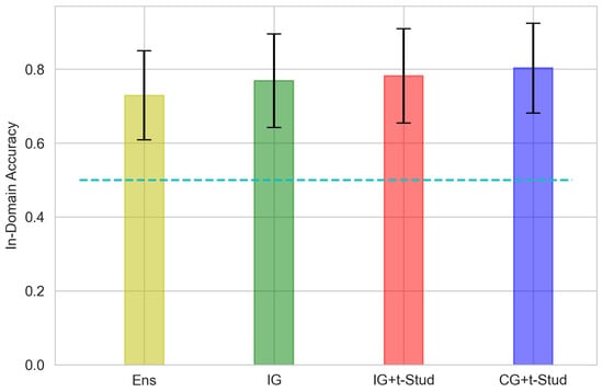
Figure 7.
Values of In-Domain 2-classes accuracy averaged across all participants, using different prior constraints compared to the ensemble for Shallow ConvNet architecture. The error bar represents the 95% confidence interval. The cyan dashed line represents the 0.5 threshold of random guessing. See Figure 3 caption for other details.
As for the experiment involving all four classes of data (Figure 8 and Figure 9), the Bayesian networks outperformed their deterministic counterparts, according to the Wilcoxon signed-rank test (EEGNet vs. Bayesian EEGNet: T = 0.0, p = 0.004, Shallow ConvNet vs. Bayesian ShallowConvNet: T = 0.0, p = 0.01).
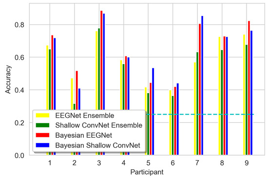
Figure 8.
The 4-classes accuracy for all participants in four classes. The cyan dashed line represents the 0.25 threshold of random guessing.
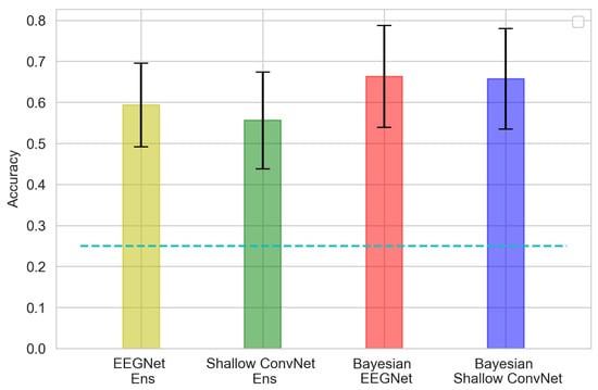
Figure 9.
The 4-classes accuracy distribution averaged across all participants. Ens stands for ‘Ensemble of 120 deterministic models’. The error bar represents the 95% confidence interval. The cyan dashed line represents the 0.25 threshold of random guessing.
3.2. Out-Of-Domain Data Detection
The bar chart, showing the distribution of ROC-AUCs of the OOD data detection method discussed above, is presented in Figure 10 and Figure 11. Unfortunately, the results of the Wilcoxon signed rank test state the absence of statistically significant differences between the ensemble and BNN under isotropic prior constraint (T = 15.0, p = 0.67) for EEGNet architecture. The same picture is for different prior constraints (IG vs. IG + t: T = 17.0, p = 0.88, IG vs. CG + t: T = 18.0, p = 0.65). Similar conclusions can be made for the Shallow ConvNet architecture (IG vs. Ensemble: T = 12.5, p = 0.25, IG vs. IG + t: T = 11.0, p = 0.33, IG vs. CG + t: T = 7.5, p = 0.07).
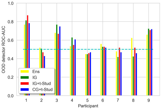
Figure 10.
ROC-AUC of OOD detection method, for all participants, using logit vector norm variance as data for different prior constraints compared to the ensemble for EEGNet architecture. Ens stands for ‘Ensemble of 120 deterministic models’, IG stands for Isotropic Gaussian prior for all layers, IG + t-Stud stands for IG for all layers and t-Student prior for the classification layer, CG + t-Stud stands for Correlated Gaussian prior for temporal and spatial convolution layers, t-Student prior for the classification layer and IG for all other layers. The cyan dashed line represents the ROC-AUC of a random classifier, which is equal to 0.5.
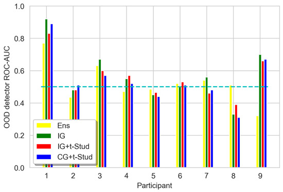
Figure 11.
ROC-AUC of OOD detection method, for all participants, using logit vector norm variance as data for different prior constraints compared to the ensemble for Shallow ConvNet architecture. The cyan dashed line represents the ROC-AUC of a random classifier, which is equal to 0.5. See Figure 9 caption for other details.
However, the average (Figure 12 and Figure 13) results are unsatisfying, though the average ROC-AUC of BNNs is slightly higher than that of the ensemble.
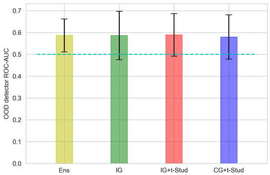
Figure 12.
ROC-AUC of OOD detection method, averaged across all participants, using logit vector norm variance as data for different prior constraints compared to the ensemble for EEGNet architecture. The error bar presents the 95% confidence interval. The cyan dashed line represents the ROC-AUC of a random classifier, which is equal to 0.5. See Figure 9 caption for other details.
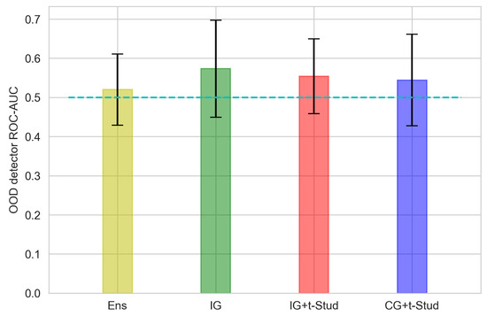
Figure 13.
ROC-AUC of OOD detection method, averaged across all participants, using logit vector norm variance as data for different prior constraints compared to the ensemble for Shallow ConvNet architecture. The error bar presents the 95% confidence interval. The cyan dashed line represents the ROC-AUC of a random classifier, which is equal to 0.5. See Figure 9 caption for other details.
4. Discussion
The first observation in this study was the increase in accuracy for the BNNs compared to baseline neural network classifiers. While this increase was not significant for the architecture based on EEGNet, it was significant for Shallow ConvNet with two of three tested priors and was especially strong for the most complex prior. This could likely happen because the most complex prior was able to capture the temporal and spatial correlation in data, providing better and smarter regularization. The higher generalization properties of the BNNs compared to their deterministic analogs have been known and already applied for BCI tasks [12,16]. Also, various Bayesian methods not involving deep learning, such as sparse Bayesian classifiers, were successfully used for BCIs for different types of brain activity, such as ERP [34] or motor imaging [35]. There were attempts to use Bayesian classifiers for online BCI experiments [36,37]. However, here, the BNNs were used for the first time, to our knowledge, for enhancing the neural network classifiers most widely used in BCI research, EEGNet, and Shallow ConvNet. Our results should be considered quite preliminary, and the results we obtained should be further verified on larger datasets collected in a number of different BCI tasks. We expect, however, that further research on the different informative prior constraints may enable additional improvement of the classification quality. One of the main objectives of this study was to test Bayesian machine learning methods on a type of data that is unconventional within the machine learning academic community. It sparked curiosity to observe how these methods, which are known for their excellent performance on benchmarks and presumed generality, would fare in a real-world machine learning environment.
While the Bayesian framework succeeded in enhancing generalization, it fell short in providing accurate uncertainty estimates, at least at the group level. This indicates that the field of EEG classification requires further adaptation of the framework to render it genuinely valuable for this specific domain. We think that the suggested method might have performed inconsistently because of the inadequate prior. The priors we used are the baseline priors in the field of image recognition. Specifically, to develop adequate priors for EEG classification tasks, one should have some expertise in the frequency and spatial distributions of the EEG signals.
The inadequate uncertainty estimation of the predictions resulted in less promising performance for out-of-distribution (OOD) detection. Our OOD detection methods failed to perform consistently, although there were some participants on which it performed well. Interestingly, the performance of the OOD detector dropped in the same participants, whereas the performance of the classifier itself was less satisfactory. Thus, it is worth assessing how the quality and non-stationarity of the input data are related to the poor performance of the OOD detector. Also, this may happen due to the suboptimal training of the classifier. This leads to the presence of the wrongly classified in-domain data on both sides of every dividing hyperplane, together with the out-of-domain data. This mixing can undermine the quality of the OOD data detector. Furthermore, we expect that the performance of the detector can be improved by hyperparameter optimization of the prior distributions’ parameters and varying the uncertainty metrics. For instance, the entropy or the likelihood may be used as such metrics.
Note that the OOD detection problem was addressed only in our study. Concerning the two other studies that dealt with uncertainty estimation, Milanes-Hermosilla et al. [12] used a similar threshold method with entropy as the uncertainty measure. However, they used that method for a different task, namely, classification with rejection. The purpose of the classification task with rejection is to reject all data with high uncertainty, i.e., where the classifier can make random predictions. It is quite closely related to the OOD data detection problem, but there are some differences. In an OOD data detection problem, one states if the sample is from a known data distribution or not, whereas in classification with a rejection problem, one needs to assign a class label to a sample if it is from the data distribution. Duan et al. [11] also studied uncertainty estimation, but they focused on its reduction. Moreover, they used a dropout for making predictions on a test set as a Bayesian feature of architecture, which is a very restricted case of the Bayesian deep learning framework.
This may raise the question of the perspectives of BNN-based OOD detection methods in BCIs, especially in online (real-time) experiments. With our hardware, it took a couple of hours to train a BNN, whereas the training of the deterministic ensemble of the same size requires less than an hour. The amounts of time consumed for the experiments’ conduction are presented in Table 2. One may refer to the variational inference methods as the faster ones, but we expect that they provide a less accurate approximation. We state that mainly relying on two arguments: firstly, the family of known distributions to approximate the posterior is quite sparse; secondly, the obtained approximations of the posterior can significantly differ from a real one [38].
Table 2.
Time consumed by classifier training for different experiments.
Interestingly, the Bayesian algorithms made from EEGNet were trained faster than the deterministic ones. It happens because we had to start training each new instance of the ensemble from randomly initialized weights, while for the Bayesian model, we just continued the same Markov chain to collect new samples of the weights.
The intractability of the integrals in Bayes’ theorem, complex approximations, and a bulky mathematical apparatus come as a hindrance to the possible successful usage of these methods in online experiments, mainly because of higher time complexity, which comes as a consequence of the architectural drawbacks. The problem of time complexity can be solved by using more modern GPUs. The complex math also may be the cause of the higher entry-level, which can affect the spreading of the BNN-based methods negatively. This might be overcome by a significant increase in the quality of classification or OOD detection quality when few learning data are available.
Irrespective of the opportunities to improve the OOD detection method we suggested here, we would like to emphasize that OOD detection methods are no less important for BCIs than for other applications. Other ways to address the OOD challenge in BCIs could develop more specific novel methods or adapt existing ones from other areas of science, for example, distance-based [39] or density-based [40].
5. Conclusions
In this study, we explored the application of Bayesian methods to wide-spread convolutional neural networks (CNNs) used for BCI (Brain–Computer Interface) classification tasks. To achieve this, we employed advanced techniques from Bayesian machine learning, such as stochastic gradient MCMC samplers, and experimented with various prior assumptions about the distribution of neural network weights. These techniques led to some improvements in the generalization properties of the models. However, the detection of out-of-distribution (OOD) input data was satisfactory only on some participants’ data. One possible reason for this could be the use of prior distributions that proved effective in uncertainty estimation for computer vision tasks but possibly are not well suited for EEG data classification. This suggests that this domain demands more specific prior constraints on model weights. In further studies, such constraints could be derived from expert knowledge in the field or by encoding functional constraints directly into the model output.
The usage of BNNs comes with increased computational complexity, which can hinder their usage for real-time experiments, but we think that this challenge could be overcome by using more modern hardware, particularly GPUs. However, we expect that real-time OOD detection is possible if the algorithm was trained in advance of the experiment.
Author Contributions
Conceptualization, B.L.K. and E.I.C.; methodology, B.L.K. and E.I.C.; supervision, B.L.K. and S.L.S.; investigation, E.I.C.; visualization, E.I.C.; software, E.I.C.; original draft writing, E.I.C.; draft revision and editing, S.L.S., B.L.K. and E.I.C.; project administration, S.L.S.; grant acquisition, S.L.S. All authors have read and agreed to the published version of the manuscript.
Funding
This research was funded by the Russian Science Foundation, grant 22-19-00528.
Data Availability Statement
The code of the experiments is available on https://github.com/CheHumbleProgger/BNN_OOD_Paper (accessed on 27 July 2023).
Conflicts of Interest
The authors declare no conflict of interest.
References
- Lotte, F.; Bougrain, L.; Cichocki, A.; Clerc, M.; Congedo, M.; Rakotomamonjy, A.; Yger, F. A review of classification algorithms for EEG-based brain–computer interfaces: A 10 year update. J. Neural Eng. 2018, 15, 031005. [Google Scholar] [CrossRef] [PubMed]
- Wojcikiewicz, W.; Vidaurre, C.; Kawanabe, M. Stationary Common Spatial Patterns: Towards robust classification of non-stationary EEG signals. In Proceedings of the 2011 IEEE International Conference on Acoustics, Speech and Signal Processing (ICASSP), Prague, Czech Republic, 22–27 May 2011; IEEE: Prague, Czech Republic, 2011; pp. 577–580. [Google Scholar]
- Zheng, Y.; Chen, G.; Huang, M. Out-of-Domain Detection for Natural Language Understanding in Dialog Systems. IEEE/ACM Trans. Audio Speech Lang. Process 2020, 28, 1198–1209. [Google Scholar] [CrossRef]
- Zeng, Z.; He, K.; Yan, Y.; Liu, Z.; Wu, Y.; Xu, H.; Jiang, H.; Xu, W. Modeling Discriminative Representations for Out-of-Domain Detection with Supervised Contrastive Learning 2021. Available online: http://arxiv.org/abs/2105.14289 (accessed on 3 August 2023).
- Ryu, S.; Koo, S.; Yu, H.; Lee, G.G. Out-of-domain Detection based on Generative Adversarial Network. In Proceedings of the Proceedings of the 2018 Conference on Empirical Methods in Natural Language Processing, Brussels, Belgium, 31 October–4 November 2018; Association for Computational Linguistics: Brussels, Belgium, 2018; pp. 714–718. [Google Scholar]
- Major, D.; Lenis, D.; Wimmer, M.; Berg, A.; Neubauer, T.; Bühler, K. On the Importance of Domain Awareness in Classifier Interpretations in Medical Imaging. IEEE Trans. Med. Imaging 2023, 42, 2286–2298. [Google Scholar] [CrossRef]
- Wellhausen, L.; Ranftl, R.; Hutter, M. Safe Robot Navigation Via Multi-Modal Anomaly Detection. IEEE Robot. Autom. Lett. 2020, 5, 1326–1333. [Google Scholar] [CrossRef]
- Caron, S.; Hendriks, L.; Verheyen, R. Rare and Different: Anomaly Scores from a combination of likelihood and out-of-distribution models to detect new physics at the LHC. SciPost Phys. 2022, 12, 77. [Google Scholar] [CrossRef]
- Maddox, W.J.; Izmailov, P.; Garipov, T.; Vetrov, D.P.; Wilson, A.G. A.G. A Simple Baseline for Bayesian Uncertainty in Deep Learning. In Advances in Neural Information Processing Systems; Wallach, H., Larochelle, H., Beygelzimer, A., Alché-Buc, F.d., Fox, E., Garnett, R., Eds.; Curran Associates, Inc.: Red Hook, NY, USA, 2019; Volume 32, Available online: https://proceedings.neurips.cc/paper_files/paper/2019/file/118921efba23fc329e6560b27861f0c2-Paper.pdf (accessed on 15 August 2023).
- Hendrycks, D.; Gimpel, K. A Baseline for Detecting Misclassified and Out-of-Distribution Examples in Neural Networks 2018. Available online: http://arxiv.org/abs/1610.02136 (accessed on 3 August 2023).
- Duan, T.; Wang, Z.; Liu, S.; Srihari, S.N.; Yang, H. Uncertainty Detection and Reduction in Neural Decoding of EEG Signals 2022. Available online: http://arxiv.org/abs/2201.00627 (accessed on 9 February 2023).
- Milanés-Hermosilla, D.; Trujillo-Codorniú, R.; Lamar-Carbonell, S.; Sagaró-Zamora, R.; Tamayo-Pacheco, J.J.; Villarejo-Mayor, J.J.; Delisle-Rodriguez, D. Robust Motor Imagery Tasks Classification Approach Using Bayesian Neural Network. Sensors 2023, 23, 703. [Google Scholar] [CrossRef]
- Jospin, L.V.; Laga, H.; Boussaid, F.; Buntine, W.; Bennamoun, M. Hands-On Bayesian Neural Networks—A Tutorial for Deep Learning Users. IEEE Comput. Intell. Mag. 2022, 17, 29–48. [Google Scholar] [CrossRef]
- Joyce, J. Bayes’ Theorem. In The Stanford Encyclopedia of Philosophy; Zalta, E.N., Ed.; Metaphysics Research Lab, Stanford University: Stanford, CA, USA, 2021; Available online: https://plato.stanford.edu/archives/fall2021/entries/bayes-theorem/ (accessed on 18 July 2023).
- Wang, H.; Yeung, D.-Y. A Survey on Bayesian Deep Learning. ACM Comput. Surv. 2021, 53, 1–37. [Google Scholar] [CrossRef]
- Li, M.; Li, F.; Pan, J.; Zhang, D.; Zhao, S.; Li, J.; Wang, F. The MindGomoku: An Online P300 BCI Game Based on Bayesian Deep Learning. Sensors 2021, 21, 1613. [Google Scholar] [CrossRef]
- Siddique, T.; Mahmud, M.S. Classification of fNIRS Data Under Uncertainty: A Bayesian Neural Network Approach 2021. Available online: http://arxiv.org/abs/2101.07128 (accessed on 28 June 2023).
- Blundell, C.; Cornebise, J.; Kavukcuoglu, K.; Wierstra, D. Weight Uncertainty in Neural Networks 2015. Available online: http://arxiv.org/abs/1505.05424 (accessed on 9 February 2023).
- Schupbach, J.; Sheppard, J.W.; Forrester, T. Quantifying Uncertainty in Neural Network Ensembles using U-Statistics. In Proceedings of the 2020 International Joint Conference on Neural Networks (IJCNN), Glasgow, UK, 19–24 July 2020; IEEE: Glasgow, UK, 2020; pp. 1–8. [Google Scholar]
- Zeng, X.; Wu, J.; Wang, D.; Zhu, X.; Long, Y. Assessing Bayesian model averaging uncertainty of groundwater modeling based on information entropy method. J. Hydrol. 2016, 538, 689–704. [Google Scholar] [CrossRef]
- Henning, C.; D’Angelo, F.; Grewe, B.F. Are Bayesian Neural Networks Intrinsically Good at Out-of-Distribution Detection? 2021. Available online: http://arxiv.org/abs/2107.12248 (accessed on 21 June 2023).
- Lawhern, V.J.; Solon, A.J.; Waytowich, N.R.; Gordon, S.M.; Hung, C.P.; Lance, B.J. EEGNet: A Compact Convolutional Network for EEG-based Brain-Computer Interfaces. J. Neural Eng. 2018, 15, 056013. [Google Scholar] [CrossRef] [PubMed]
- Schirrmeister, R.T.; Springenberg, J.T.; Fiederer, L.D.J.; Glasstetter, M.; Eggensperger, K.; Tangermann, M.; Hutter, F.; Burgard, W.; Ball, T. Deep learning with convolutional neural networks for EEG decoding and visualization: Convolutional Neural Networks in EEG Analysis. Hum. Brain Mapp. 2017, 38, 5391–5420. [Google Scholar] [CrossRef] [PubMed]
- Brunner, C.; Leeb, R.; Müller-Putz, G.; Schlögl, A.; Pfurtscheller, G. BCI Competition 2008–Graz Data Set A; Institute for Knowledge Discovery (Laboratory of Brain-Computer Interfaces), Graz University of Technology: Styria, Austria, 2008; Volume 16, pp. 1–6. [Google Scholar]
- Fortuin, V.; Garriga-Alonso, A.; Ober, S.W.; Wenzel, F.; Rätsch, G.; Turner, R.E.; van der Wilk, M.; Aitchison, L. Bayesian Neural Network Priors Revisited 2022. Available online: http://arxiv.org/abs/2102.06571 (accessed on 9 February 2023).
- Springenberg, J.T.; Klein, A.; Falkner, S.; Hutter, F. Bayesian Optimization with Robust Bayesian Neural Networks. In Advances in Neural Information Processing Systems; Lee, D., Sugiyama, M., Luxburg, U., Guyon, I., Garnett, R., Eds.; Curran Associates, Inc.: Red Hook, NY, USA, 2016; Volume 29, Available online: https://proceedings.neurips.cc/paper_files/paper/2016/file/a96d3afec184766bfeca7a9f989fc7e7-Paper.pdf (accessed on 18 July 2023).
- Loshchilov, I.; Hutter, F. Decoupled Weight Decay Regularization 2019. Available online: http://arxiv.org/abs/1711.05101 (accessed on 11 July 2023).
- Paszke, A.; Gross, S.; Massa, F.; Lerer, A.; Bradbury, J.; Chanan, G.; Killeen, T.; Lin, Z.; Gimelshein, N.; Antiga, L.; et al. Pytorch: An imperative style, high-performance deep learning library. Adv. Neural Inf. Process. Syst. 2019, 32, 8024–8035. [Google Scholar]
- Gramfort, A. MEG and EEG data analysis with MNE-Python. Front. Neurosci. 2013, 7, 267. [Google Scholar] [CrossRef] [PubMed]
- Hunter, J.D. Matplotlib: A 2D Graphics Environment. Comput. Sci. Eng. 2007, 9, 90–95. [Google Scholar] [CrossRef]
- Waskom, M. seaborn: Statistical data visualization. JOSS 2021, 6, 3021. [Google Scholar] [CrossRef]
- Virtanen, P.; Gommers, R.; Oliphant, T.E.; Haberland, M.; Reddy, T.; Cournapeau, D.; Burovski, E.; Peterson, P.; Weckesser, W.; Bright, J.; et al. SciPy 1.0: Fundamental algorithms for scientific computing in Python. Nat Methods 2020, 17, 261–272. [Google Scholar] [CrossRef]
- Tran, B.-H.; Rossi, S.; Milios, D.; Filippone, M. All You Need is a Good Functional Prior for Bayesian Deep Learning. J. Mach. Learn. Res. 2022, 23, 1–56. [Google Scholar]
- Zhang, Y.; Zhou, G.; Jin, J.; Zhao, Q.; Wang, X.; Cichocki, A. Sparse Bayesian Classification of EEG for Brain–Computer Interface. IEEE Trans. Neural Netw. Learning Syst. 2016, 27, 2256–2267. [Google Scholar] [CrossRef]
- Wang, W.; Qi, F.; Wipf, D.; Cai, C.; Yu, T.; Li, Y.; Yu, Z.; Wu, W. Sparse Bayesian Learning for End-to-End EEG Decoding. IEEE Trans. Pattern Anal. Mach. Intell. 2023, 1–18. [Google Scholar] [CrossRef]
- Higger, M.; Quivira, F.; Akcakaya, M.; Moghadamfalahi, M.; Nezamfar, H.; Cetin, M.; Erdogmus, D. Recursive Bayesian Coding for BCIs. IEEE Trans. Neural Syst. Rehabil. Eng. 2017, 25, 704–714. [Google Scholar] [CrossRef] [PubMed]
- Sun, S.; Lu, Y.; Chen, Y. The stochastic approximation method for adaptive Bayesian classifiers: Towards online brain–computer interfaces. Neural Comput. Applic 2011, 20, 31–40. [Google Scholar] [CrossRef]
- Blei, D.M.; Kucukelbir, A.; McAuliffe, J.D. Variational Inference: A Review for Statisticians. J. Am. Stat. Assoc. 2017, 112, 859–877. [Google Scholar] [CrossRef]
- Chen, X.; Lan, X.; Sun, F.; Zheng, N. A Boundary Based Out-of-Distribution Classifier for Generalized Zero-Shot Learning 2022. Available online: http://arxiv.org/abs/2008.04872 (accessed on 7 July 2023).
- Tonin, F.; Pandey, A.; Patrinos, P.; Suykens, J.A.K. Unsupervised Energy-based Out-of-distribution Detection using Stiefel-Restricted Kernel Machine. In Proceedings of the 2021 International Joint Conference on Neural Networks (IJCNN), Shenzhen, China, 18–22 July 2021; IEEE: Shenzhen, China, 2021; pp. 1–8. [Google Scholar]
Disclaimer/Publisher’s Note: The statements, opinions and data contained in all publications are solely those of the individual author(s) and contributor(s) and not of MDPI and/or the editor(s). MDPI and/or the editor(s) disclaim responsibility for any injury to people or property resulting from any ideas, methods, instructions or products referred to in the content. |
© 2023 by the authors. Licensee MDPI, Basel, Switzerland. This article is an open access article distributed under the terms and conditions of the Creative Commons Attribution (CC BY) license (https://creativecommons.org/licenses/by/4.0/).