CTprintNet: An Accurate and Stable Deep Unfolding Approach for Few-View CT Reconstruction

Abstract

In this paper, we propose a new deep learning approach based on unfolded neural networks for the reconstruction of X-ray computed tomography images from few views. We start from a model-based approach in a compressed sensing framework, described by the minimization of a least squares function plus an edge-preserving prior on the solution. In particular, the proposed network automatically estimates the internal parameters of a proximal interior point method for the solution of the optimization problem. The numerical tests performed on both a synthetic and a real dataset show the effectiveness of the framework in terms of accuracy and robustness with respect to noise on the input sinogram when compared to other different data-driven approaches.

1. Introduction

It is very important to have reliable and trustworthy methods to obtain good X-ray computed tomography (CT) scans with the lowest level of radiation to achieve medical diagnoses. A common strategy, known as sparse-view CT, reduces the radiation dose by capturing a limited number of data. The CT imaging process can mathematically be expressed as the following model:

$$y=\mathcal{D}\left(H\overline{x}\right),$$

(1)

where $\overline{x}\in {\mathbb{R}}^n$ is the image we want to reconstruct, $y\in {\mathbb{R}}^m$ is the acquired data (also called a sinogram), $\mathcal{D}$ is the noise perturbation, and $H\in {\mathbb{R}}^{m\times n}$ is the linear tomographic operator. Due to the limited number of data, the sparse-view CT problem can be cast into the compressed sensing framework [1,2], which includes a large variety of imaging problems, e.g., diffuse optic tomography [3], magnetic resonance imaging [4], image deblurring [5], optical coherence tomography [6], and synthetic-aperture radar imaging [7].

In addition to being indeterminate, the inverse problem (1) is typically also ill-conditioned, and the more traditional analytical methods such as filtered back projection (FBP) produce images dominated by noise and artifacts. An efficient alternative to invert (1) is the model-based approach, where an iterative algorithm solves a minimization problem by incorporating prior information on the reconstruction as either regularization functions or constraint. Among the several proposals in literature, the total variation (TV) function is certainly the most widely used in medical CT (see, e.g., [8]). The advantages of model-based methods are their explainability and the data consistency imposed by the physical model. However, they require hard parameter tuning and a long execution time.

In the last decade, motivated by the availability of huge datasets and new efficient computational devices, such as dedicated graphics processing units (GPUs), deep neural networks (DNNs), in particular convolutional neural networks (CNNs), have been successfully employed for X-ray CT image reconstruction, producing very accurate reconstructions at the expense of explainability and robustness to noise. Deep-learning-based methods used for CT can be grouped into four classes. The first class is called data-to-image, and here, the neural network directly maps the acquired sinogram to the reconstructed image (see, for example, [9]). This approach is not widely used since it is well known that it is not stable with respect to noise in the data [10]. The second class is composed of networks directly mapping coarse reconstructed images to accurate reconstructions, and for this reason, it is named image-to-image. Most of the proposed methods use CNNs, taking as input FBP reconstructions (see, e.g., [11,12,13]). The third class is the plug-and-play-type approaches, where a network is trained outside of the iterative process and then included within it, thus allowing the iteration to be run indefinitely [14,15,16]. The last approach is known as iterative mapping, and it is realized through the so-called unrolled (or unfolded) neural networks [17]. The aim of these methods is to mimic the action of a minimization problem by simultaneously learning the hyper-parameters of the model, such as the regularization hyper-parameters, the iterative solution algorithms, and/or the model operators.

The first deep unfolding networks were applied to specific inverse problems [18], and they demonstrated improved performance compared to the more traditional optimization algorithms. Since then, deep unfolding has been extended to compressive sensing [19,20], image deblurring [21], and tomographic image reconstruction. To cite some examples, the first proposals were from J. Adler and O. Öktem in [22,23], where they unrolled a proximal primal–dual method. More recent works are: (a) [24], which concerns the fast iterative shrinkage/thresholding algorithm (FISTA), which can be applied to solve CT and electromagnetic tomography reconstruction problems; (b) [25], in which a few iterations of a gradient descent method were applied to a field-of-experts regularized least squares functional; and (c) [26], where the authors unfolded the dual block forward–backward (DBFB) algorithm embedded in an iterative re-weighted scheme for region-of-interest CT image reconstruction. A different scheme is investigated in [27], where the pseudodifferential operator is learned for limited-angle CT.

The unfolding-deep-learning-based approach is of great interest to the mathematical community and for scientific research since, by exploiting the physical model of the CT inversion and the regularization properties imposed on the solution by the prior, it maintains coherence between the reconstruction and the sinogram; therefore, it is more explainable and exhibits higher stability properties than other deep learning methods.

Contributions. The aim of this work is to propose an accurate and robust unfolded approach, named CTprintNet in the following, for the reconstruction of CT images from sparse views. The main ingredients of the CTprintNet architecture are those of the iRestNet approach, proposed in [21] for image deblurring, which unrolls the proximal interior point algorithm for the solution of a regularized minimization problem and learns the regularization parameter of the model, as well as two more proper parameters of the algorithm. We consider as prior a smooth generalization of the TV regularizer, which is very effective in medical imaging, in particular in CT, at both reducing the noise and preserving the edges of objects, such as masses or fibers, which is useful for diagnosis [28,29,30].

We conducted tests of CTprintNet in the presence of different noise intensities with respect to the noise used for training to check the stability property of the framework. Our network proves to be very stable with respect to the noise on the input sinogram; when compared to an image-to-image method, it shows greater robustness with respect to noise.

Organization of the paper. This paper is organized as follows. In Section 2, we briefly recall the CT imaging problem and reformulate it as an inverse problem. The optimization method exploited to address its solution is detailed in Section 3, while the CTprintNet architecture built by unfolding the iterations of this method is illustrated in Section 4, together with some implementation choices made for the numerical tests. The experimental results are presented in Section 5. Finally, some concluding remarks and considerations are given in Section 6.

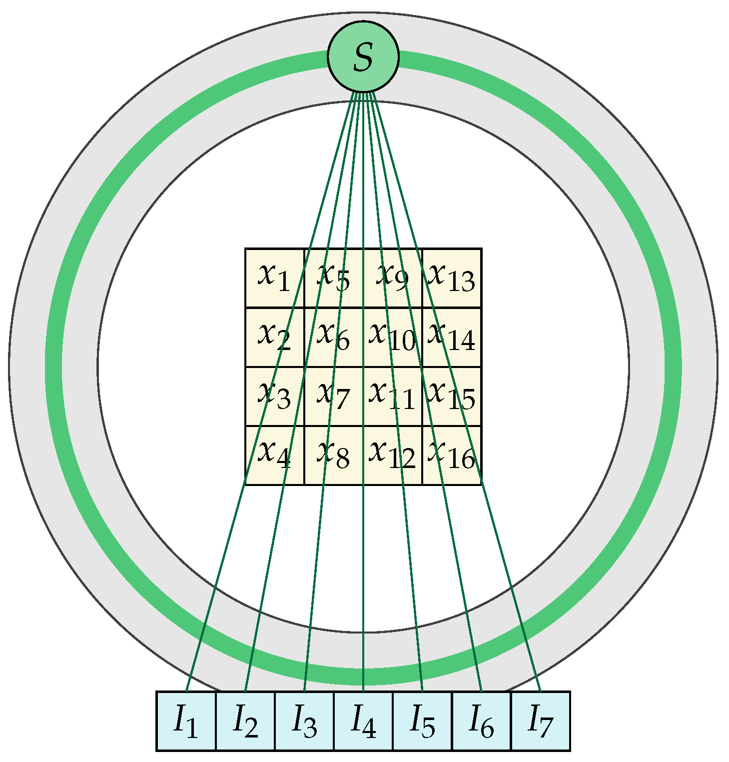
2. The Numerical Model

In this section, we briefly introduce a description of the 2D X-ray CT acquisition process, including some mathematical notations.

The main focus of CT studies is to develop safer protocols to reduce the radiation dose for the patient since limiting the negative effects produced by the radiation allows the use of the CT technique in a wider class of medical examinations. This goal can be pursued by either decreasing the X-ray tube current at each scan (low-dose CT) or reducing the number of X-ray projections (few-view CT). In the first case, the measured data present high levels of noise; however, in the second case, the incompleteness of the projection data leads to create images with pronounced artifacts. In particular, in this paper, we focus on the few-view CT case, where image reconstruction is particularly difficult.

Over the years, different tomographic devices have been designed to fit different medical needs, and this has led to the creation of various protocols and geometries. In particular, in this study, we focus on fan-beam geometry, schematized in Figure 1, since it is among the most widespread geometries nowadays. It is characterized by a source that emits fan-beam X-rays whose intensity is recorded, after passing through a body, by a decoder with $N_p$ elements.

The aim of CT imaging is to reconstruct the attenuation coefficient function $\mu (x,y)$ of the object when passing through a body from the $N_{\theta }$ projections acquired at equally spaced ${\theta }_k$ angles, with $k=1,\cdots ,N_{\theta }$, and performed in the angular range $[-\mathsf{\Theta },\mathsf{\Theta }]$ (in our case, $\mathsf{\Theta }=\frac{\pi }{2}$). Each individual projection is modelled by the Radon transform, which is the integral along the line L describing the path of an X-ray beam at a fixed angle. According to Beer–Lambert’s law, given $I_0$ as the intensity emitted by the X-ray source and I as the intensity measured by the detector, we have

$$-ln\left(\frac{I}{I_0}\right)={\int }_L\mu (x,y)d(x,y).$$

(2)

In the real (discrete) case, the function $\mu (x,y)$, which describes the object, is discretized in $N=N_x\times N_y$ pixels, with values that can be lexicographically re-ordered in a vector $x\in {\mathbb{R}}^N$.

Analysing a single projection acquired at a fixed angle ${\theta }_k$ from $N_p$ cells of the decoder, Equation (2) can be discretized into a sum over all the pixels as

$$y_i^{{\theta }_k}=\sum _{j=1}^N{H}_{i,j}^{{\theta }_k}{x}_{j}i=1,\cdots ,N_p$$

(3)

where $y_i^{{\theta }_k}=-ln\left(\frac{I_i}{I_0}\right)$ and $I_i$ is the intensity measured by the i-th cell. Repeating for all the angles ${\theta }_k$, with $k=1,\cdots ,N_{\theta }$, and using a compact notation, we obtain the linear system

$$y=Hx,$$

(4)

where $x\in {\mathbb{R}}^N$ denotes the CT image to be reconstructed, $y\in {\mathbb{R}}^{N_d}$ is the synogram obtained with the projection measurements (with $N_d=N_{\theta }\times N_p$), and $H\in {\mathbb{R}}^{N_d\times N}$ is a sparse matrix representing the discrete line integrals in (2). Hence, tomographic image reconstruction is mathematically modeled as an ill-conditioned inverse problem, whose solutions can be dominated by noise. In particular, in the few-view CT case, the linear system is also under-determined due to the lack of projections, and, therefore, it might have infinite solutions.

The model-based approach is introduced to address these numerical controversies, with the aim to model the CT imaging process as a minimization problem of a suitable cost function. The main idea is to combine a fidelity measure on the data with some a priori information on the solution, thus leading to the following problem:

$$\underset{x\in {\mathbb{R}}^N}{argmin}f(Hx,y)+\lambda \mathcal{R}\left(x\right)$$

(5)

where $f:{\mathbb{R}}^N\to \mathbb{R}$ is the data-fidelity term, $\mathcal{R}:{\mathbb{R}}^N\to \mathbb{R}$ is a regularization function, and $\lambda \in (0,+\infty )$ is the regularization parameter.

The data-fitting function is related to the statistics of the noise on the data, and we consider the least squares function

$$f(Hx,y)={\parallel Hx-y\parallel }_2^2,$$

(6)

which provides a good maximum a posteriori estimate for the log-Poisson noise affecting the measured sinograms [31]. Different functions have been proposed in the CT literature as regularization terms. In particular, the TV function is suitable for use with tomographic images that are rather uniform inside the organs while having fast variations on the borders. Since, in our scheme, we need the objective function in (5) to be differentiable, we consider a smoothed version of the TV function, defined as

$$T{V}_{\delta }\left(x\right)=\sum _{j=1}^N\sqrt{{\left(D_{h}x\right)}_j^2+{\left(D_{v}x\right)}_j^2+{\delta }^2}$$

(7)

where $D_h,D_v\in {\mathbb{R}}^{N\times N}$ are the horizontal and vertical gradient operators, respectively, and $\delta$ is a small positive parameter. Finally, hard constraints on the values of the image’s pixels are typically added to preserve the physical properties of the attenuation coefficients. A standard assumption is to force the solution to belong to the N-dimensional hypercube $\mathcal{C}={[0,1]}^N$, thus leading to the constrained optimization problem

$$\underset{x\in {[0,1]}^N}{argmin}{\parallel Hx-y\parallel }_2^2+\lambda T{V}_{\delta }\left(x\right).$$

(8)

3. Proximal Interior Point Method for CT Reconstruction

Problem (8) involves the constrained minimization of a smooth and convex objective function, which can be performed by means of a large variety of optimization methods. In our paper, we consider the proximal interior point approach [32], in which the original constrained minimization problem (8) is replaced by a sequence of unconstrained problems

$$\underset{x\in {\mathbb{R}}^N}{argmin}{\parallel Hx-y\parallel }_2^2+\lambda T{V}_{\delta }\left(x\right)+\mu \mathcal{B}\left(x\right),$$

(9)

where $\mathcal{B}:{\mathbb{R}}^N\to \mathbb{R}\cup \{+\infty \}$ is the logarithmic barrier function, defined as

$$\mathcal{B}\left(x\right)=\left\{\begin{array}{cc}-\sum _{j=1}^N(ln\left(x_j\right)+ln(1-x_j))\hfill & x\in {(0,1)}^N\hfill \\ +\infty \hfill & \mathrm{otherwise},\hfill \end{array}\right.$$

(10)

and $\mu \in (0,+\infty )$ is the barrier parameter, which goes to zero along the minimization.

Following [21], we address the minimization of (9) by means of the forward–backward proximal interior point (FBPIP) method, whose iterations are defined in Algorithm 1, where

$${\mathrm{prox}}_{\mu \mathcal{B}}\left(x\right)=\underset{u\in {\mathbb{R}}^n}{\mathrm{argmin}}\frac{1}{2}{\parallel x-u\parallel }^2+\mu \mathcal{B}\left(u\right)$$

(11)

is the proximity operator of $\mu \mathcal{B}$ at x [33].

The following proposition directly derives from ([21], Proposition 2); we report its statement and proof adapted to problem (9) and (10) to show the closed-form expression of the proximal point defining $x_{k+1}$ in Algorithm 1, together with its derivatives with respect to x, $\mu$, and $\gamma$.

Algorithm 1: Proximal interior point algorithm.

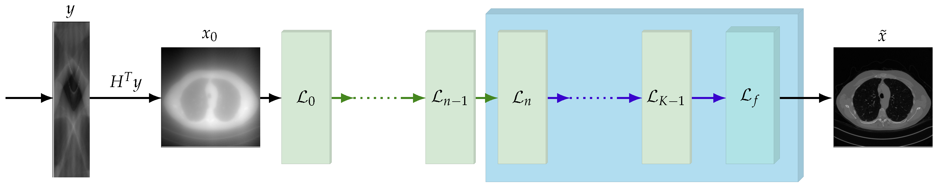
Let $x_0\in \mathrm{int}\mathcal{C}$, $\underline{\gamma }>0$ and ${\left({\gamma }_k\right)}_{k\in \mathbb{N}}$ be a sequence such that $(\forall k\in \mathbb{N})$$\underline{\gamma }\le {\gamma }_k$; for$k=0,1,\dots$do    $x_{k+1}={\mathrm{prox}}_{{\gamma }_k{\mu }_k\mathcal{B}}\left(x_k-{\gamma }_k\left(H^{\top }(H{x}_k-y)+\lambda \nabla T{V}_{\delta }\left(x_k\right)\right)\right)$ end for

Proposition 1.

Let $\gamma ,\mu >0$ and let ${\mathcal{B}}_i\left(u\right)$ be the barrier function associated with the set $[0,1]$, defined as

$${\mathcal{B}}_i\left(u\right)=\left\{\begin{array}{cc}-ln\left(1-u_i\right)-ln\left(u_i\right)\hfill & \mathrm{if}0<u_i<1\hfill \\ +\infty \hfill & \mathit{otherwise}\hfill \end{array}\right..$$

(12)

Then, for every $x\in {\mathbb{R}}^N$, the proximity operator associated with $\gamma \mu {\mathcal{B}}_i$ is given by

$${\phi }_i(x,\mu ,\gamma ):={\mathrm{prox}}_{\gamma \mu {\mathcal{B}}_i}\left(x\right)=x+(\kappa (x,\mu ,\gamma )-u_i)e_i,$$

(13)

where $\kappa (x,\mu ,\gamma )$ is the unique solution in $(0,1)$ of the cubic equation

$$z^3-\left(1+u_i\right)z^2+\left(u_i-2\gamma \mu \right)z+\gamma \mu =0$$

(14)

and $e_i$ is the i-th vector of the canonical basis of ${\mathbb{R}}^N$. The Jacobian matrix of φ with respect to x and the gradients of φ with respect to μ and γ are given by

$$J_{\left(x\right)}{\phi }_i(x,\mu ,\gamma )={\mathbb{I}}_n+\left(\frac{\kappa (x,\mu ,\gamma )\left(\kappa \right(x,\mu ,\gamma )-1)}{\eta (x,\mu ,\gamma )}-1\right)e_i{e}_i^T$$

(15)

$${\nabla }_{\left(\mu \right)}{\phi }_i(x,\mu ,\gamma )=\frac{-\gamma (1-2\kappa (x,\mu ,\gamma \left)\right)}{\eta (x,\mu ,\gamma )}{e}_i$$

(16)

$${\nabla }_{\left(\gamma \right)}{\phi }_i(x,\mu ,\gamma )=\frac{-\mu (1-2\kappa (x,\mu ,\gamma \left)\right)}{\eta (x,\mu ,\gamma )}{e}_i$$

(17)

where

$$\eta (x,\mu ,\gamma )=\kappa (x,\mu ,\gamma )(\kappa (x,\mu ,\gamma )-1)-(1-2\kappa (x,\mu ,\gamma ))(\kappa (x,\mu ,\gamma )-x_i)-2\gamma \mu .$$

(18)

Proof. 

The formal derivation of the proximity operator (13) can be found in [34]. Let $x\in {\mathbb{R}}^N$, $\gamma ,\mu \in (0,+\infty )$, and F be defined as

$$\begin{array}{cc}\hfill F(x,\mu ,\gamma ,z)& =z(z-1)(z-x_i)+\gamma \mu (1-2z)\end{array}$$

(19)

$$\begin{array}{cc}& =z^3-(x_i+1)z^2+(x_i-2\gamma \mu )z+\gamma \mu \end{array}$$

(20)

for all $z\in (0,1)$. By definition of $\kappa (x,\mu ,\gamma )$, $F(x,\mu ,\gamma ,\kappa (x,\mu ,\gamma \left)\right)=0$. The derivative of F with respect to the last variable is equal to

$${\nabla }_{\left(z\right)}F(x,\mu ,\gamma ,z)=z(z-1)-(1-2z)(z-x_i)-2\gamma \mu .$$

(21)

We observe that both $\kappa (x,\mu ,\gamma )\left(\kappa \right(x,\mu ,\gamma )-1)$ and $-2\gamma \mu$ are negative quantities. Moreover, since $F(x,\mu ,\gamma ,\kappa (x,\mu ,\gamma \left)\right)=0$, it follows from (19) that $\kappa (x,\mu ,\gamma )-x_i$ and $1-2\kappa (x,\mu ,\gamma )$ share the same sign. Hence,

$$\eta (x,\mu ,\gamma )=\nabla F_{\left(z\right)}(x,\mu ,\gamma ,\kappa (x,\mu ,\gamma )\ne 0.$$

(22)

The gradient of $\kappa$ with respect to x and the partial derivatives of $\kappa$ with respect to $\mu$ and $\gamma$ for the implicit function theorem exist and are equal to

$${\nabla }_{\left(x\right)}\kappa (x,\mu ,\gamma )=\frac{\kappa (x,\mu ,\gamma )\left(\kappa \right(x,\mu ,\gamma )-1)}{\eta (x,\mu ,\gamma )}{e}_i$$

(23)

$${\nabla }_{\left(\mu \right)}\kappa (x,\mu ,\gamma )=\frac{-\gamma (1-2\kappa (x,\mu ,\gamma \left)\right)}{\eta (x,\mu ,\gamma )}$$

(24)

$${\nabla }_{\left(\gamma \right)}\kappa (x,\mu ,\gamma )=\frac{-\mu (1-2\kappa (x,\mu ,\gamma \left)\right)}{\eta (x,\mu ,\gamma )}$$

(25)

Using these equations to differentiate (13) leads to the results of the proposition.    □

We end this section by remarking that, since the barrier function $\mathcal{B}$ in (10) is the sum of the functions ${\mathcal{B}}_i$ in (12) and each of these acts only on the i-th component of the vector u, then the proximity operator associated to $\gamma \mu \mathcal{B}$ is the vector $\phi (x,\mu ,\gamma )\in {\mathbb{R}}^N$, defined as

$${\left(\phi (x,\mu ,\gamma )\right)}_i:={\phi }_i(x,\mu ,\gamma )\forall i\in \{1,\dots ,N\}.$$

(26)

4. CTprintNet

We now describe the proposed CTprintNet, which unfolds in its layers the FBPIP iterations. As mentioned in the Introduction, its architecture reflects that of iRestNet, which is used for the deblurring of natural images and was described in Section 4.1, with the obvious modification of starting from the sinograms instead of the blurred images. The main differences between the two approaches can be seen in the implementation of the forward operator and its adjoint, as well as the consequent setting of all the hyperparameters, which will be discussed in Section 4.2. The whole architecture was implemented in Python using the PyTorch library.

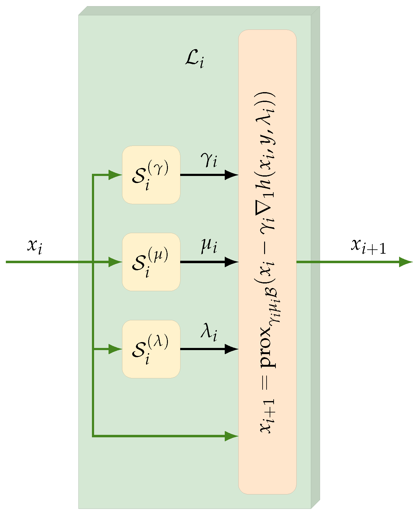
4.1. CTprintNet Architecture

Figure 2 shows the flowchart describing the architecture. It is composed of K iterative layers $({\mathcal{L}}_0,\dots ,{\mathcal{L}}_{K-1})$ and a final block of post-processing layers $\left({\mathcal{L}}_f\right)$. In each layer, the network learns three parameters, which are supposed to change at each algorithm iteration: the regularization parameter $\lambda$ (which was supposed constant in the model description in Section 3), the stepsize $\gamma$, and the barrier parameter $\mu$. Since the simultaneous optimization of the parameters of all the K layers is infeasible due to memory issues, for the first n layers ${\left({\mathcal{L}}_i\right)}_{0\le i\le n-1}$, a greedy approach is adopted throughout the training by sequentially optimizing the output of each iteration and providing it as the starting image for the following iteration. The remaining $K-n$ layers and the final layer, the light blue block in Figure 2, are trained in a standard end-to-end way and will later be referred to as ${\mathcal{L}}_n\circ \cdots \circ {\mathcal{L}}_{K-1}\circ {\mathcal{L}}_f$.

In all our tests, we kept the original choice of iRestNet by setting $K=40$ and $n=30$.

Regarding the details of the construction of one iterative layer ${\left({\mathcal{L}}_i\right)}_{0\le i\le K-1}$, as can be seen from Figure 3, it is composed of three substructures, denoted by $({\mathcal{S}}_i^{\left(\gamma \right)},{\mathcal{S}}_i^{\left(\mu \right)},{\mathcal{S}}_i^{\left(\lambda \right)})$, inferring the step size ${\gamma }_i$, the barrier parameter ${\mu }_i$, and the regularization parameter ${\lambda }_i$, respectively. They are constructed by analyzing the mathematical constraint imposed on the three parameters.

In particular, for all $i=0,\dots ,K-1$:

•

Since the step size ${\gamma }_i$ must be positive, this constraint is imposed by estimating the step size as

$${\gamma }_i={\mathcal{S}}_i^{\left(\gamma \right)}=\mathrm{Softplus}\left(a_i\right),$$

(27)

where $a_i$ is a scalar parameter of the architecture learned during the training and the $\mathrm{Softplus}$ function is defined as

$$\mathrm{Softplus}\left(z\right)=ln(1+exp(z\left)\right)\forall z\in \mathbb{R};$$

(28)

•

The barrier parameter ${\mu }_i$ is computed by twice alternating a convolutional layer and an average pooling layer, followed by a fully connected layer and a final Softplus activation function;

•

The regularization parameter ${\lambda }_i$ is estimated as follows:

$${\lambda }_i={\mathcal{S}}_i^{\left(\lambda \right)}\left(x_i\right)=\frac{\mathrm{Softplus}\left(b_i\right)\widehat{\sigma }\left(y\right)}{\eta \left(x_i\right)+\mathrm{Softplus}\left(c_i\right)},\widehat{\sigma }\left(y\right)=\mathrm{median}\left(\right|W_{H}y\left|\right)/0.6745,$$

(29)

where $\eta \left(x_i\right)$ is the standard deviation of the concatenated spatial gradients of $x_i$, $(b_i,c_i)$ are scalars learned by the architecture, and $|W_{H}y|$ is the absolute value of the diagonal coefficients of the first-level Haar wavelet decomposition of y. The rationale behind this choice is to provide an initial guess from the ratio between the estimated data fidelity magnitude and the regularizer magnitude (represented by the noise level and the gradient variations, respectively), suitably adjusted by two learned constants.

The outputs of the three substructures are then used to compute $x_{k+1}$ by applying an iteration of the iterative method, Algorithm 1, as shown in Figure 3.

Since some initial convergence issues were encountered in a (very) limited number of tests, in CTprintNet, we introduced a quality check on the output image of the very first layer ${\mathcal{L}}_0$, requiring it to exceed a minimum value of mean square error. If this test fails, ${\mathcal{L}}_0$ is re-trained with different random initializations.

The network is completed by the final block, as displayed in Figure 4, which acts as a form of post-processing to enhance the quality of the image obtained from the iterative layers. It is built with nine convolutional layers with filters of size $3\times 3$ with a different dilation factor between one and the other; each layer is followed by a ReLU activation function and batch normalization. At the end of these layers, there is a skip connection between the input and output of the block and a final sigmoid activation function.

4.2. Forward/Backward Operators and Hyper-Parameter Setting

The iterative methods for the reconstruction of tomographic images require two linear operators, usually referred to as the forward and the backward (or back-projection) projectors, which describe the geometry and the physics of the problem. In order to make the best use of the hardware and the memory hierarchy, it is common to use different discretization techniques for the two operators. This choice implies that the standard routines implementing discretized versions of the Radon transform and its adjoint (such as, e.g., the radon and iradon functions in Matlab’s Image Processing Toolbox and Python’s scikit-image one) lead to an unmatched projector/back-projector pair, in which the matrix representing the back-projection is not exactly equal to the transposed matrix of the projector operator. Although this mismatch contributes to speeding every iteration up and to reducing the global computational cost, it can lead to a less accurate reconstruction since the convergence properties of the iterative method are lost [35,36]. In order to overcome this issue, we discretized the projection operator with a ray tracing algorithm and stored it in memory as a sparse row matrix, H. We then used its exact transpose, $H^T$, as a back-projection. Since we could not make use of the built-in implementation of the PyTorch functions acting on tensors, we implemented the functions necessary to compute the partial derivatives, which are essential during the back-propagation algorithm.

This choice represents the crucial difference with respect to iRestNet, in which this matter was not an issue since the convolution operator and its adjoint can be easily and exactly executed through fast Fourier transforms and the conjugate operator. Moreover, it strongly affects the choice of some hyper-parameters, such as the number of epochs and the batch size, which had to be set to lower values with respect to the iRestNet values due to the lower amount of available memory, especially in the end-to-end training of the final ${\mathcal{L}}_n\circ \cdots \circ {\mathcal{L}}_{K-1}\circ {\mathcal{L}}_f$ block. Their final values, together with the learning rate values, were set following several experimental tests and are reported in

Table 1. Training hyper-parameters.

Parameters	${\mathcal{L}}_0$	${\left({\mathcal{L}}_{\mathit{i}}\right)}_{1\le \mathit{i}\le 29}$	${\mathcal{L}}_{30}\circ \cdots \circ {\mathcal{L}}_{39}\circ {\mathcal{L}}_{\mathit{f}}$
epochs	5	10	50
batchsize	8	8	5
learning rate	${10}^{-1}$	${10}^{-2}$	${10}^{-1}$

.

All the training and tests of the network were performed on an Nvidia RTX A4000 GPU. We have chosen the mean square error (MSE) as a loss function in the learning process and stochastic gradient descent as an optimizer, which performed better with respect to the structural similarity index measure (SSIM) and the Adam optimizer exploited in iRestNet.

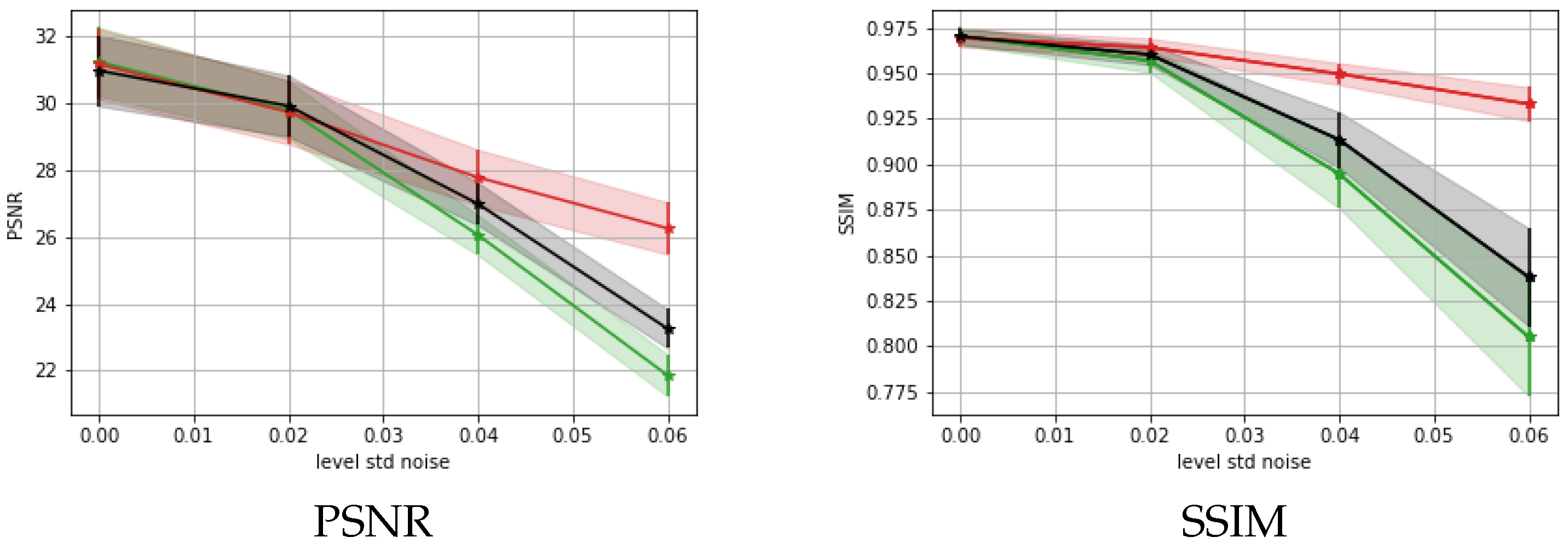
5. Results and Discussion

In this section, we show and analyze the performance of the proposed CTprintNet architecture for two different datasets composed of synthetic images with geometric elements and real medical images. Let us first describe the training procedure and the experimental setting.

In all the implemented experiments, we used the same protocol to simulate the few-view geometry, i.e., a reduced scanning trajectory limited to 180 degrees with $N_{\theta }=60$ scanning views that were equally distributed, with $n_p=512$ and $n_p=1024$ for the synthetic and realistic datasets, respectively. We constructed the test problem as

$$\tilde{y}=Hx+\mathcal{N}(0,\sigma )·N_{\theta },$$

(30)

where $\mathcal{N}(0,\sigma )$ is a realization of a normally distributed random variable with a mean equal to zero and a standard deviation equal to $\sigma$. As we will see in the results, different values of $\sigma$ were considered in the training and testing phases. The sinogram was then used to compute the first iteration $x_0=H^{T}y$.

The results obtained with the proposed architecture were compared with both an iterative solver and a deep learning approach. For the first class of methods, we chose the scaled gradient projection method (SGP) [37], which has already been used several times to reconstruct CT images [38,39,40]. Regarding the choice of a competitor among the deep learning methods, it has been very hard for us to exploit existing unfolding architectures specifically designed for tomographic image reconstruction problems. Although algorithms of this type can be found in the literature (see, e.g., the references cited in the Introduction), the codes required to produce the results either are not available or require a notable amount of modifications to be usable. As a result of this, we decided to compare CTprintNet with an image-to-image approach constituted of a UNet residual network applied to a coarse FBP reconstruction. We will denote this framework as LPP in the following. In particular, the different LPP trainings were carried out on the same datasets used for CTprintNet by performing 100 epochs for the synthetic dataset and 50 for the realistic one.

We evaluated the performances through qualitative visual comparisons and by quantitatively computing the peak signal-to-noise ratio (PSNR) and the SSIM [41].

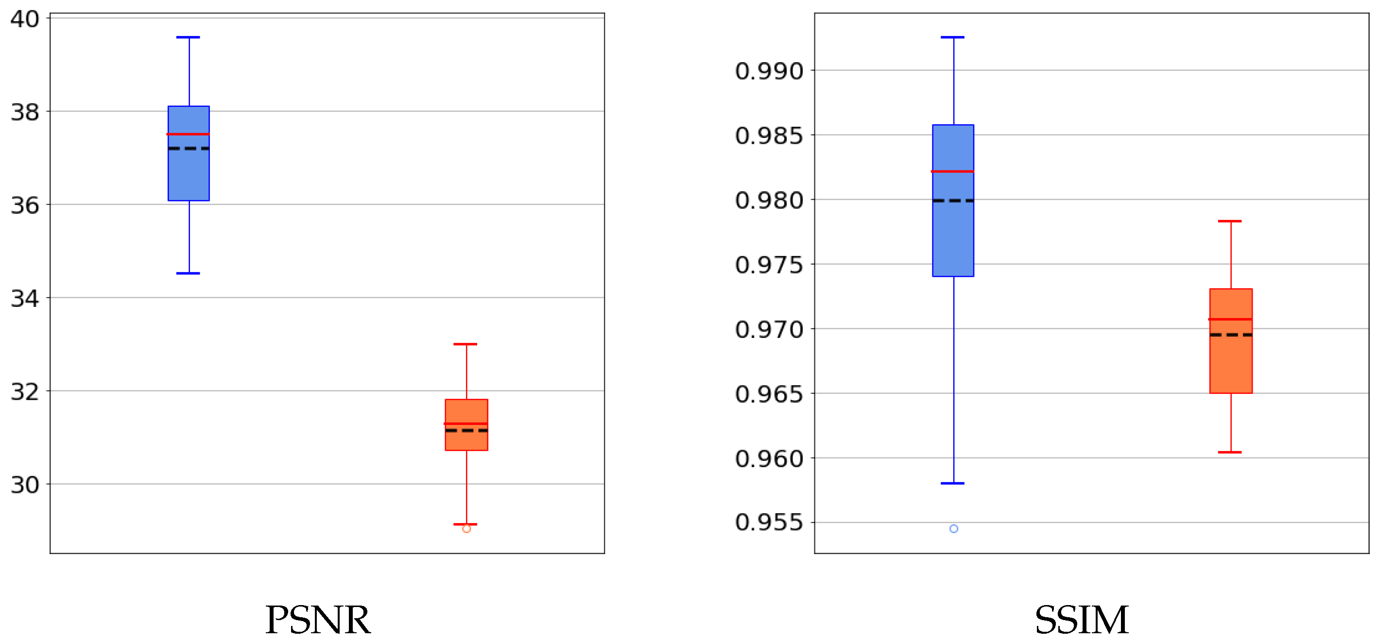
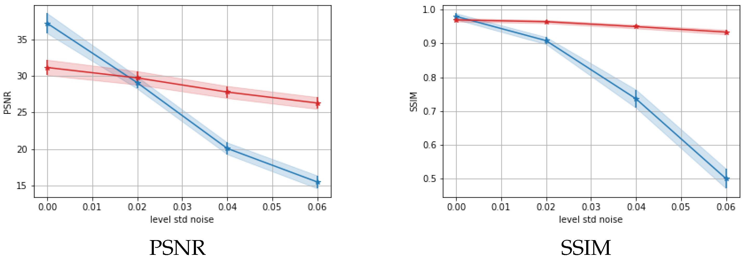
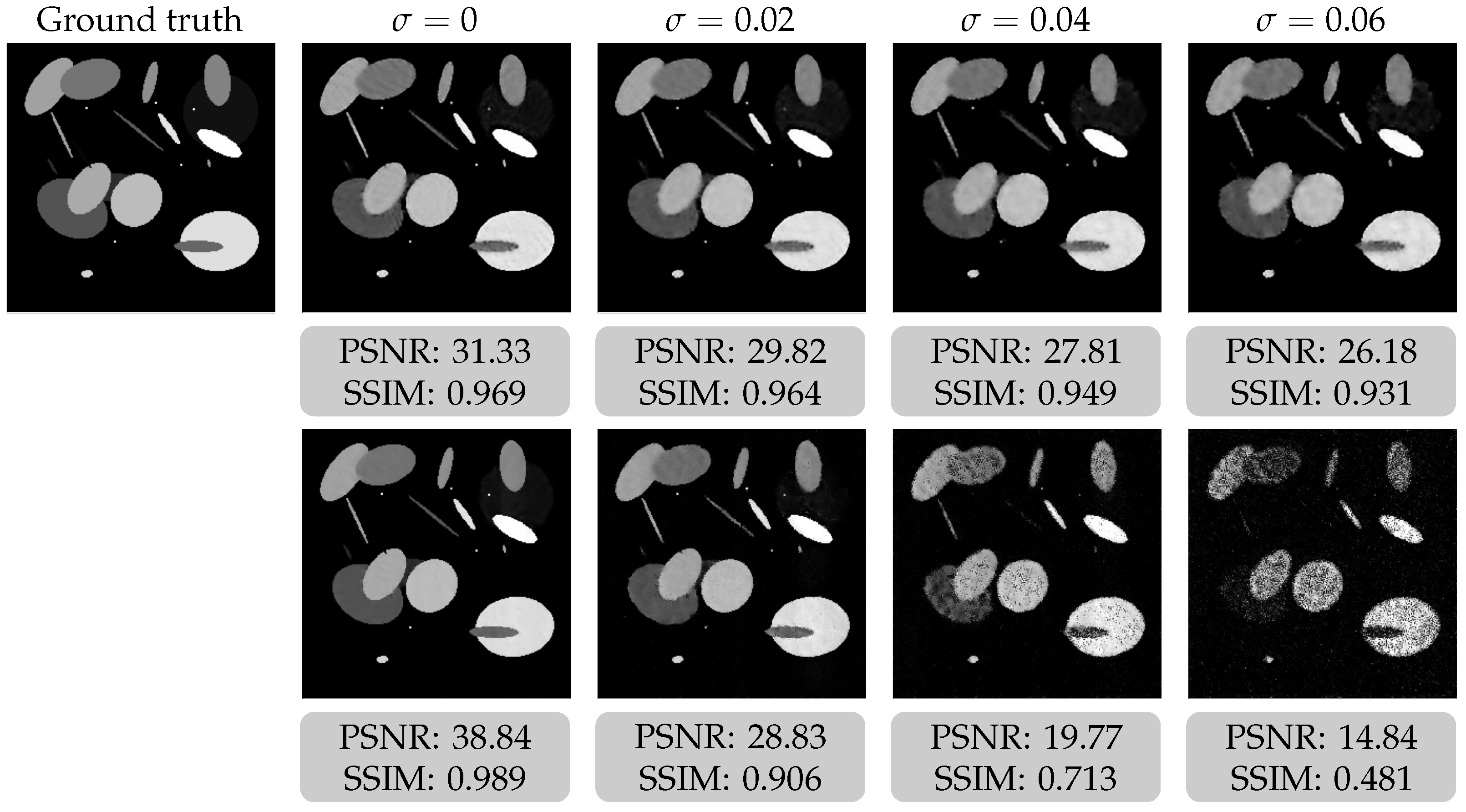
5.1. Results on a Synthetic Dataset

We first tested the algorithms on the synthetic dataset “Contrasted Overlapping Uniform Lines and Ellipses” (COULE) (https://www.kaggle.com/datasets/loiboresearchgroup/coule-dataset, accessed on 13 November 2021), which contains 430 sparse-gradient grayscale images of size $256\times 256$. Among the 430 images, we used 400 for training and the remaining 30 for the test phase.

Experiment A. In this experiment, we trained and tested CTprintNet and LPP considering data without noise. From Figure 5, showing the boxplots relative to PSNR, SSIM (in blue for LPP and in orange for CTprintNet), we can see that LPP defines better reconstructions, on average. In fact, it is well known that the post-processing architectures perform particularly well in standard conditions where the training and testing data are obtained from similar conditions.

Experiment B. Under real conditions, however, the projection data are naturally compromised by noise. To test the stability of the proposed framework with respect to noise in the sinogram, we first analyzed the behavior of the architecture when varying the values of the noise’s standard deviation $\sigma$ introduced in the training and test phases. In Experiment B, we trained the two architectures by adding Gaussian noise as in (30) with $\sigma =0.05$ both to the training set and test set. The results obtained, shown in Figure 6, demonstrate that noise influences the performance of the two architectures, which now are more competitive with each other. In particular, the SSIM index, indicating the visual quality of the image, is far better for CTprintNet.

Experiment C. Since it is well known that a drawback of neural networks, particularly post-processing ones, is that their performance on data never seen or far from the training data is not always satisfying, in Experiment C, we trained the two architectures without noise on the data ($\sigma =0$), and we tested them with variable standard deviations in the interval $[0,0.06]$. In Figure 7, we plot the average values of the two metrics as the standard deviation of the noise added on the test set changes (the blue and red lines correspond to LPP and CTprintNet, respectively). The results clearly show that the proposed architecture is stable with respect to noise, whereas the LPP initially provides better performance; however, as the noise increases, its behavior worsens considerably (see also the reconstructions of a representative test image in Figure 8). Conversely, CTprintNet is able to guarantee good results by limiting the damage caused by increased noise despite being trained with noise-free images.

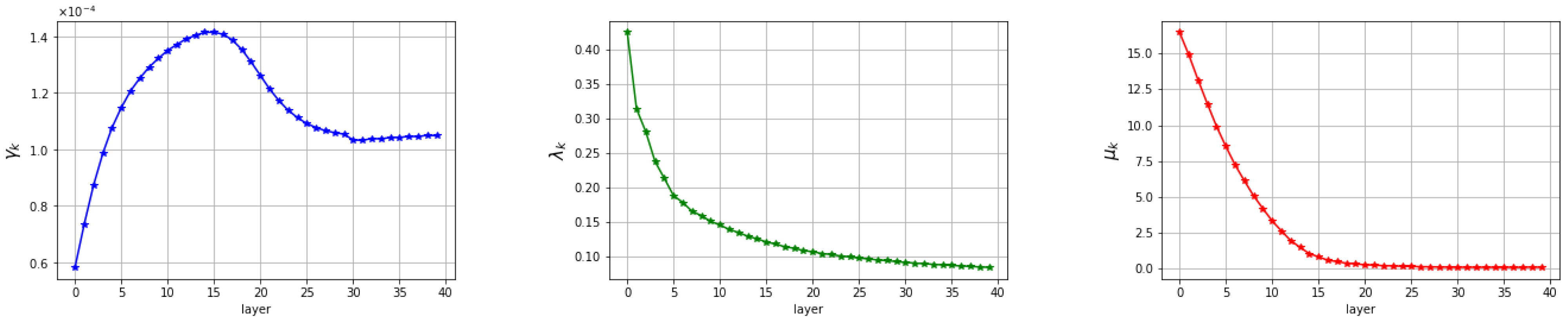
5.2. Discussion of the Learned Parameters

In this section, we study how the choice of $\lambda$ affects the performance of the network by examining a further learning technique and providing a brief excursus on the behavior of the three learned parameters. To this aim, we initially fixed $\lambda$, as it happens in general in the iterative method, while the remaining parameters ($\mu ,\gamma$) were learned from the architecture. We performed Experiment C with different values of $\lambda$ set by analyzing those learned from the network in previous experiments, and we saved the best-performing values.

We then utilized a different technique, described in [42,43], for learning the regularization parameter, leaving the techniques used to learn $\mu$ and $\gamma$ untouched. The idea behind this technique is to provide a local TV regularization by setting a specific parameter for each pixel, thus obtaining a weighted TV (WTV), as follows:

$$WTV\left(x\right)=\sum _{i=1}^N{\lambda }_i\sqrt{{\left(D_{h}x\right)}_i^2+{\left(D_{v}x\right)}_i^2}.$$

(31)

This choice allows to diversify the level of the regularization within the single image, e.g., by regularizing more on constant patches and less on patches with complex textures. From the implementation point of view, the parameters ${\lambda }_i$ ($i=1,\dots ,N$) in the k-th layer for the i-th pixel are computed as

$${\lambda }_i^{\left(k\right)}=\frac{\mathrm{Softplus}\left(d_i\right)}{2N}\frac{\left|\right|H{x}_k-y{\left|\right|}_2^2}{\sqrt{{\left(D_h{x}_k\right)}_i^2+{\left(D_v{x}_k\right)}_i^2}},$$

(32)

where $d_i$ is a scalar parameter of the architecture learned during the training. In this way, the smaller the gradient magnitude is, the greater the regularization provided at pixel i is.

We modified the architecture using this procedure for the computation of $\lambda$ in the substructure ${\mathcal{S}}^{\left(\lambda \right)}$ in Figure 3 and carried out several trainings. What is evident is that, although the architecture with this modification is able to yield slightly better performances than those obtained with the technique described in (32), it becomes worse in terms of stability.

We plot in Figure 9 the results obtained from Experiment C with a fixed $\lambda$ (black line), with Equation (29) (red line) and with Equation (32) (green line). They show that the proposed new learning rule weakens the network stability.

Next, we analyzed the behavior of the parameters learned from the architecture within the different layers. We observed from all the performed experiments that these parameters show very similar trends regardless of the image and the presence or absence of noise. In Figure 10, we plot the values, obtained from Experiment B, of the three parameters as the iterations increase. Concerning the step size, it initially increases, and then it decreases and stabilizes. The central panel of Figure 10 shows that the regularization parameter tends to vanish as the layers advance since the presence of noise decreases; as a result of this, the contribution of the regularization term becomes weaker. Finally, the barrier parameter vanishes along the minimization process according to the theoretical issues presented in Section 3.

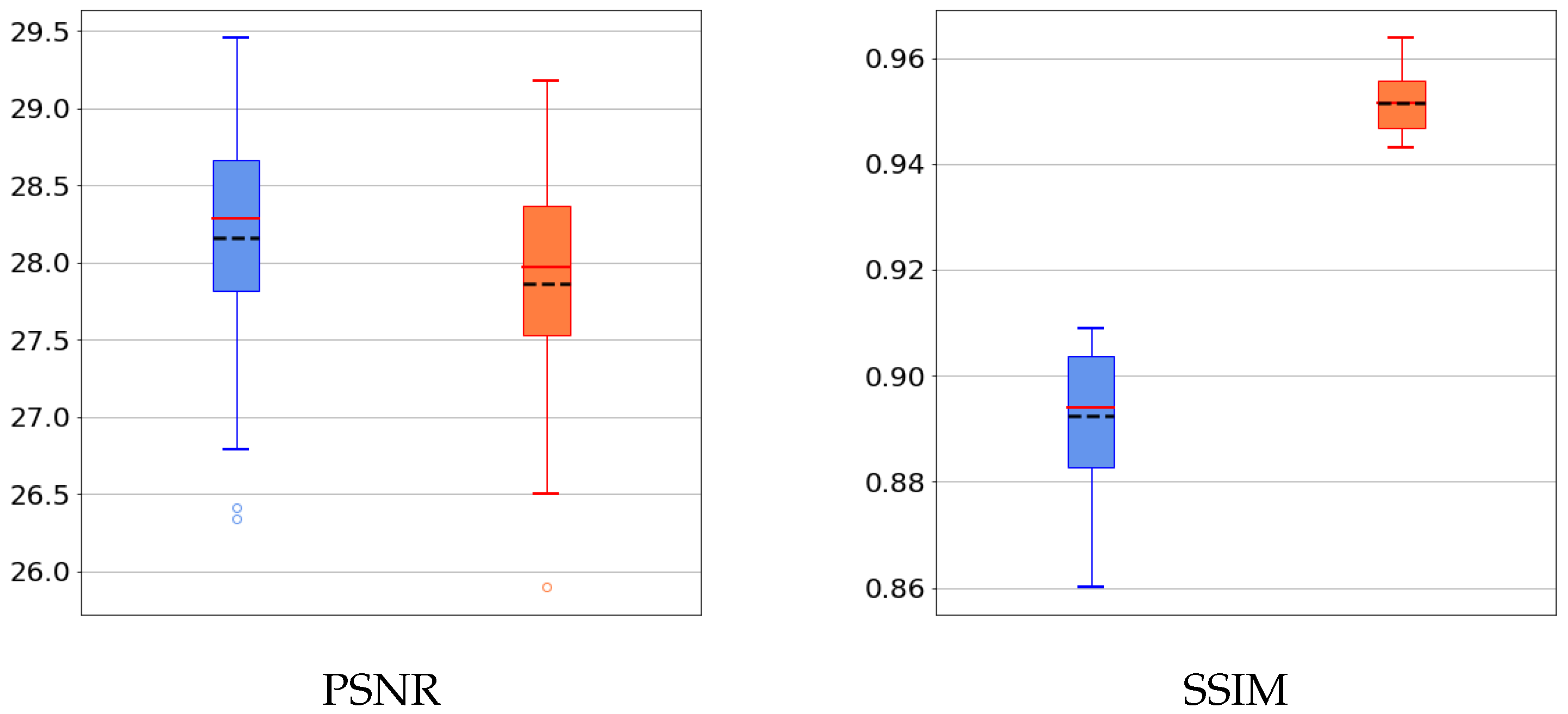
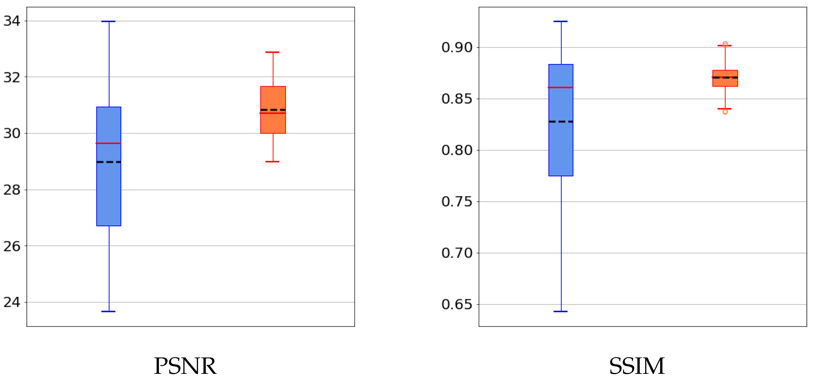
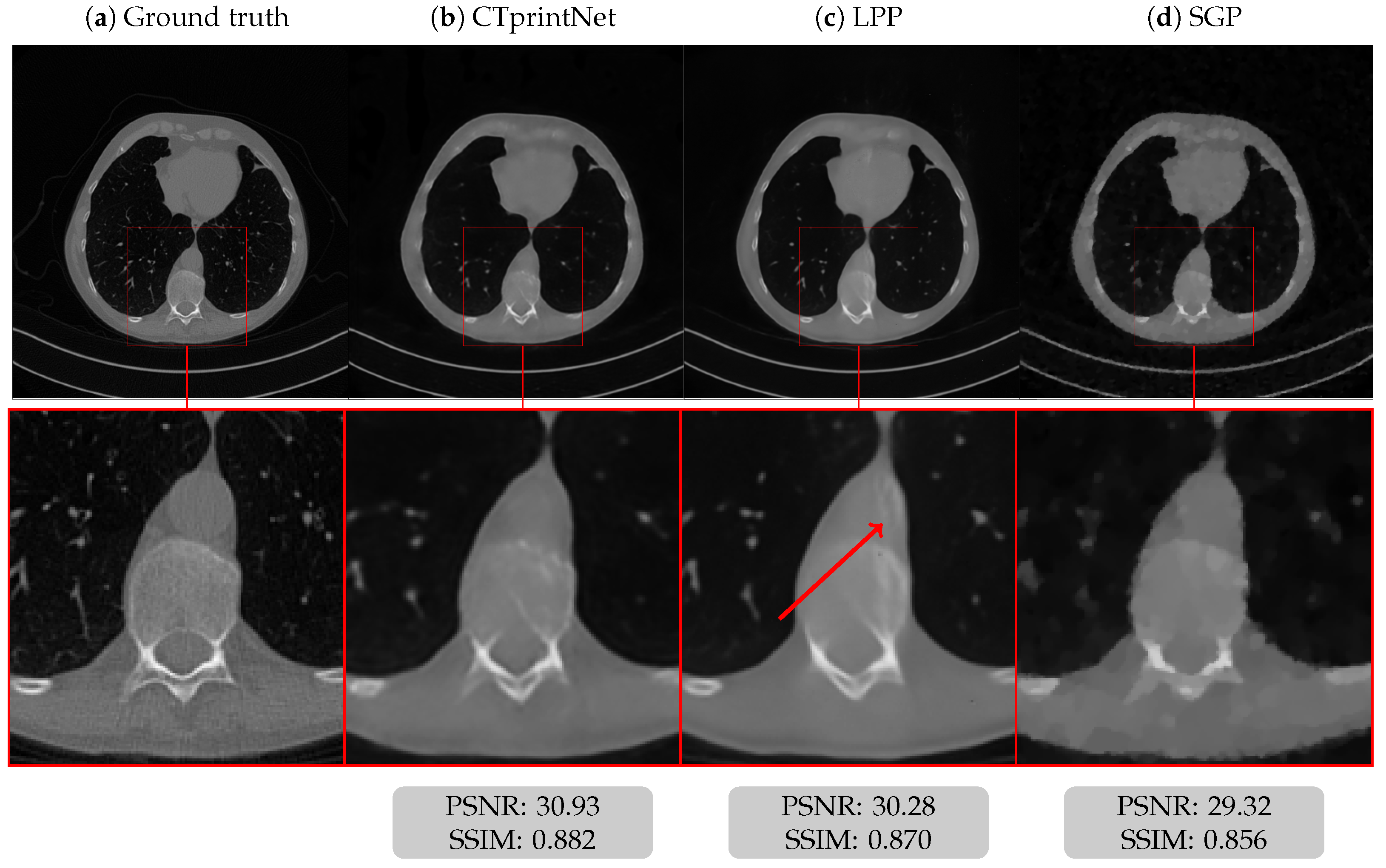
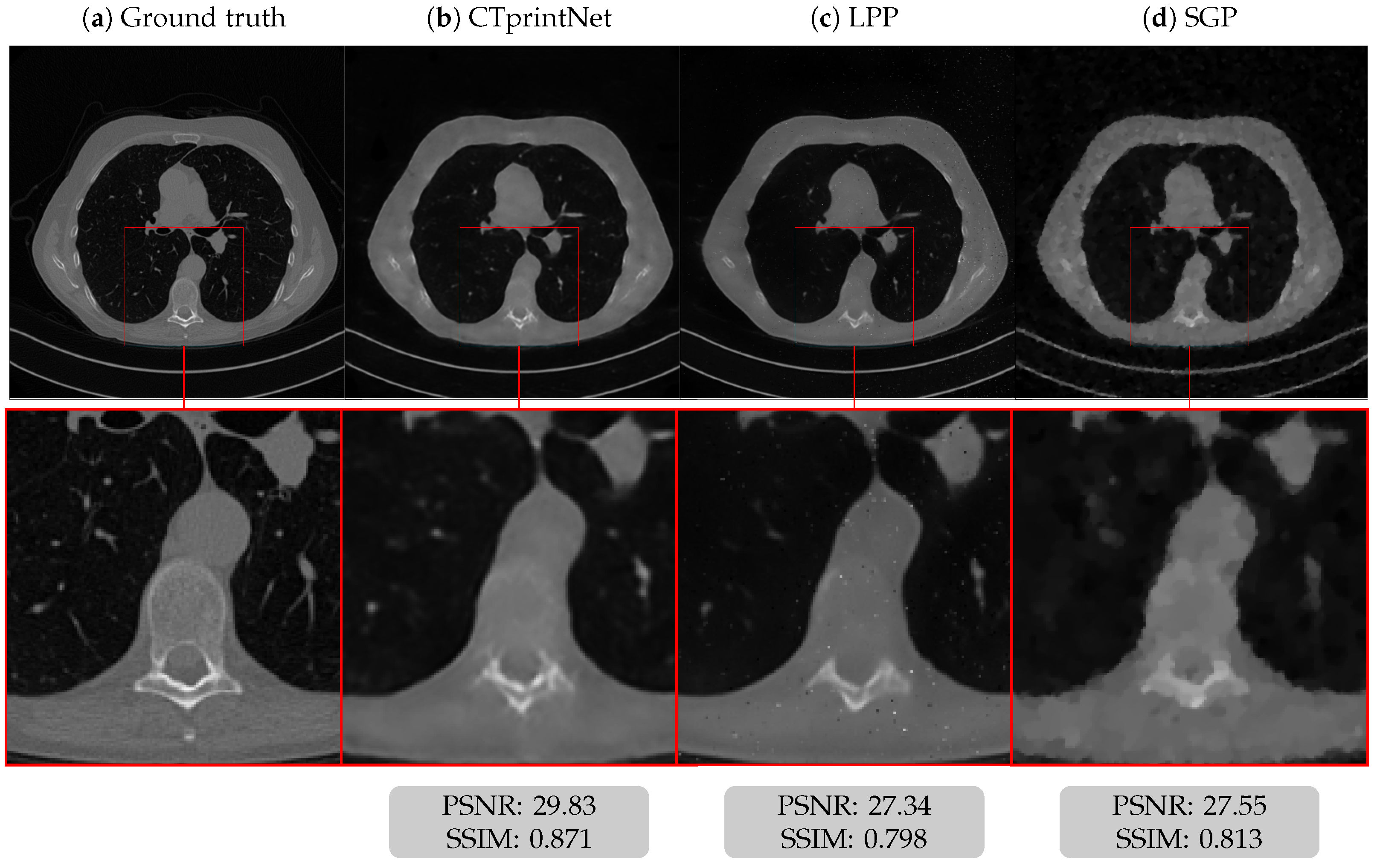
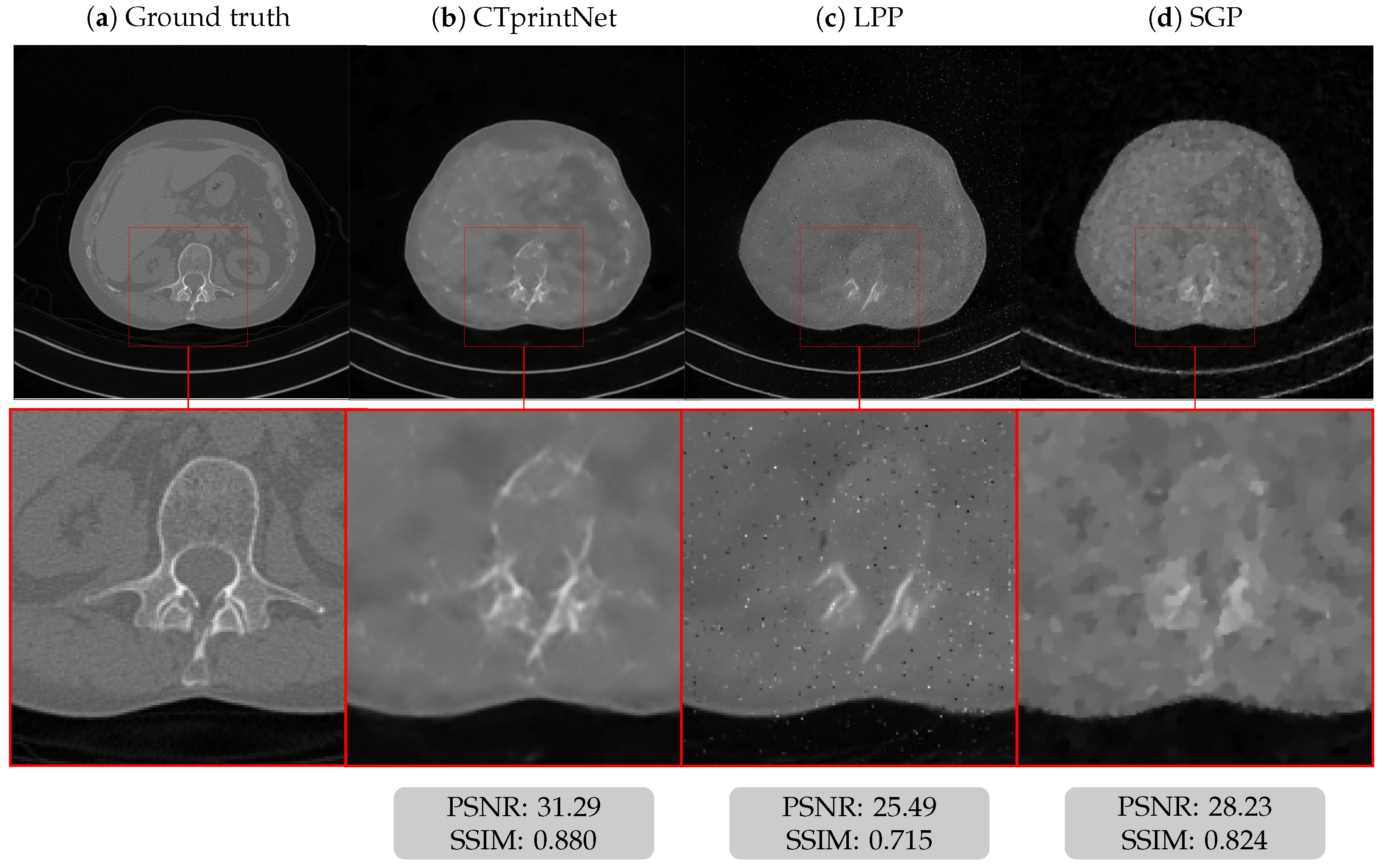
5.3. Results on a Realistic Dataset

As our realistic dataset, we used a set of clinical images from the AAPM Low-Dose CT Grand Challenge dataset by the Mayo Clinic (https://www.aapm.org/GrandChallenge/LowDoseCT/, accessed on 22 May 2023). This datset contains images of the human abdomen with a size of $512\times 512$ pixels obtained from full-dose acquisitions. From the entire dataset, we selected about 1500 images for the training phase and 327 for the testing phase.

Experiment D. In this experiment, we trained the two architectures on data affected by noise with a standard deviation $\sigma =0.05$ and tested them on data with noise with $\sigma$ chosen randomly in the range $[0.04,0.08]$. Figure 11 shows the boxplots relative to the considered metrics in blue for LPP and in orange for CTprintNet. As can be seen from the boxplots, CTprintNet obtains better performances on average; in addition, it is also more stable with respect to different noise intensities. Moreover, we observe that CTprintNet boxplots are smaller with closer means and medians with respect to the LPP boxplots, confirming its superior stability.

In the following, we will show and comment on three reconstructions obtained from test images with standard deviation values of 0.04, 0.065, and 0.075. We compared the reconstructions obtained from the proposed method with those obtained from the SGP algorithm where the regularization parameter was selected according to the high PSNR among 20 different tested values. The reconstructions from CTprintNet and LPP were obtained by considering the same training as before.

Reconstruction D.1. This example is obtained from a test image corrupted by noise with variance $\sigma =0.04$. Figure 12 depicts the reconstructed images and reports, for each one, the values of PSNR and SSIM. We observe that both CTprintNet and LPP effectively remove the typical artifacts of the few-view geometry and, in particular, they suppress the noise. However, in the LPP image, a white ghost detail appears. The SGP reconstruction looks blocky, and many details in the dark background are lost.

Reconstruction D.2. The second example is obtained from a test image corrupted by noise with variance $\sigma =0.065$. Figure 13 depicts the reconstructed images and reports, for each one, the values of PSNR and SSIM. The image obtained from the LPP framework presents over-smoothing and some incorrect pixels, as can be highlighted by the zoomed-in image. Hence, we can infer that CTprintNet reconstruction is advantageous over the other methods in terms of both metrics and noise reduction.

Reconstruction D.3. The last example is obtained from a test image corrupted by the highest amount of noise with a variance of $\sigma =0.075$. Figure 14 shows that, despite the excessive noise compared to that used in the training, the proposed network is able to provide the best-quality reconstruction. In particular, the SGP image is extremely blocky, as in the previous case, and the LPP image presents again an excessive amount of smoothing and number of corrupted pixels.

The results obtained from the various experiments on the realistic dataset confirmed that our architecture is stable, as already observed in Section 5.1.

6. Conclusions

In this paper, we have proposed CTprintNet, a neural network for the reconstruction of CT images from few views. CTprintNet fixes the low-sample problem in a compressed sensing setting by means of the total variation prior, which is achieved by unrolling the proximal interior point method. A final post-processing phase is used to enhance the reconstructed image’s quality. The network has been tested on both simulated and real test sets, with particular attention paid to its robustness with respect to unseen noise in the input data. Compared with a more traditional image-to-image deep-learning-based approach, it shows greater stability without requiring a higher amount of computational effort. The very promising results open this neural network to possible future improvements, such as the introduction of a different regularizer than TV or extension to the 3D case using a lighter network architecture.

References

1. Candès, E.J.; Romberg, J.K.; Tao, T. Robust uncertainty principles: Exact signal reconstruction from highly incomplete frequency information. IEEE Trans. Inf. Theory 2006, 52, 489–509. [Google Scholar] [CrossRef]
2. Donoho, D.L. Compressed sensing. IEEE Trans. Inf. Theory 2006, 52, 1289–1306. [Google Scholar] [CrossRef]
3. Süzen, M.; Giannoula, A.; Durduran, T. Compressed sensing in diffuse optical tomography. Opt. Express 2010, 18, 23676–23690. [Google Scholar] [CrossRef] [PubMed]
4. Montefusco, L.B.; Lazzaro, D.; Papi, S.; Guerrini, C. A fast compressed sensing approach to 3D MR image reconstruction. IEEE Trans. Med. Imaging 2011, 30, 1064–1075. [Google Scholar] [CrossRef]
5. Rostami, M.; Michailovich, O.V.; Wang, Z. Image Deblurring Using Derivative Compressed Sensing for Optical Imaging Application. IEEE Trans. Image Process. 2012, 21, 3139–3149. [Google Scholar] [CrossRef] [PubMed]
6. Mohan, N.; Stojanovic, I.; Karl, W.C.; Saleh, B.E.A.; Teich, M.C. Compressed sensing in optical coherence tomography. In Proceedings of the Three-Dimensional and Multidimensional Microscopy: Image Acquisition and Processing XVII; Conchello, J.A., Cogswell, C.J., Wilson, T., Brown, T.G., Eds.; International Society for Optics and Photonics, SPIE: Bellingham, WA, USA, 2010; Volume 7570, p. 75700L. [Google Scholar]
7. Uğur, S.; Arıkan, O. SAR image reconstruction and autofocus by compressed sensing. Digit. Signal Process. 2012, 22, 923–932. [Google Scholar] [CrossRef]
8. Hauptmann, A.; Hämäläinen, K.; Harhanen, L.; Kallonen, A.; Niemi, E.; Siltanen, S. Total variation regularization for large-scale X-ray tomography. Int. J. Tomogr. Simul. 2014, 25, 1–25. [Google Scholar]
9. He, J.; Wang, Y.; Ma, J. Radon inversion via deep learning. IEEE Trans. Med. Imaging 2020, 39, 2076–2087. [Google Scholar] [CrossRef]
10. Antun, V.; Renna, F.; Poon, C.; Adcock, B.; Hansen, A.C. On instabilities of deep learning in image reconstruction and the potential costs of AI. Proc. Natl. Acad. Sci. USA 2020, 117, 30088–30095. [Google Scholar] [CrossRef]
11. Jin, K.H.; McCann, M.T.; Froustey, E.; Unser, M. Deep convolutional neural network for inverse problems in imaging. IEEE Trans. Image Process. 2017, 26, 4509–4522. [Google Scholar] [CrossRef]
12. Chen, H.; Zhang, Y.; Kalra, M.K.; Lin, F.; Chen, Y.; Liao, P.; Zhou, J.; Wang, G. Low-dose CT with a residual encoder-decoder convolutional neural network. IEEE Trans. Med. Imaging 2017, 36, 2524–2535. [Google Scholar] [CrossRef] [PubMed]
13. Morotti, E.; Evangelista, D.; Loli Piccolomini, E. A green prospective for learned post-processing in sparse-view tomographic reconstruction. J. Imaging 2021, 7, 139. [Google Scholar] [CrossRef] [PubMed]
14. Gupta, H.; Jin, K.H.; Nguyen, H.Q.; McCann, M.T.; Unser, M. CNN-based projected gradient descent for consistent CT image reconstruction. IEEE Trans. Med. Imaging 2018, 37, 1440–1453. [Google Scholar] [CrossRef] [PubMed]
15. Lunz, S.; Öktem, O.; Schönlieb, C.B. Adversarial Regularizers in Inverse Problems. In Proceedings of the 32nd International Conference on Neural Information Processing Systems, Montreal, QC, Canada, 2–8 December 2018; NIPS’18. pp. 8516–8525. [Google Scholar]
16. Chang, J.R.; Li, C.L.; Póczos, B.; Vijaya Kumar, B.; Sankaranarayanan, A.C. One Network to Solve Them All—Solving Linear Inverse Problems Using Deep Projection Models. In Proceedings of the 2017 IEEE International Conference on Computer Vision (ICCV), Venice, Italy, 22–29 October 2017; pp. 5889–5898. [Google Scholar]
17. Monga, V.; Li, Y.; Eldar, Y.C. Algorithm Unrolling: Interpretable, Efficient Deep Learning for Signal and Image Processing. IEEE Signal Process. Mag. 2021, 38, 18–44. [Google Scholar] [CrossRef]
18. Gregor, K.; LeCun, Y. Learning Fast Approximations of Sparse Coding. In Proceedings of the 27th International Conference on Machine Learning, Haifa, Israel, 21–24 June 2010; ICML’10. pp. 399–406. [Google Scholar]
19. Zhang, J.; Ghanem, B. ISTA-Net: Interpretable optimization-inspired deep network for image compressive sensing. In Proceedings of the 2018 IEEE/CVF Conference on Computer Vision and Pattern Recognition (CVPR), Salt Lake City, UT, USA, 18–23 June 2018; pp. 1828–1837. [Google Scholar]
20. Yang, Y.; Sun, J.; Li, H.; Xu, Z. ADMM-CSNet: A deep learning approach for image compressive sensing. IEEE Trans. Pattern Anal. Mach. Intell. 2018, 42, 521–538. [Google Scholar] [CrossRef] [PubMed]
21. Bertocchi, C.; Chouzenoux, E.; Corbineau, M.C.; Pesquet, J.C.; Prato, M. Deep unfolding of a proximal interior point method for image restoration. Inverse Probl. 2020, 36, 034005. [Google Scholar] [CrossRef]
22. Adler, J.; Öktem, O. Solving ill-posed inverse problems using iterative deep neural networks. Inverse Probl. 2017, 33, 124007. [Google Scholar] [CrossRef]
23. Adler, J.; Öktem, O. Learned Primal-Dual Reconstruction. IEEE Trans. Med. Imaging 2018, 37, 1322–1332. [Google Scholar] [CrossRef]
24. Xiang, J.; Dong, Y.; Yang, Y. FISTA-Net: Learning a fast iterative shrinkage thresholding network for inverse problems in imaging. IEEE Trans. Med. Imaging 2021, 40, 1329–1339. [Google Scholar] [CrossRef]
25. Chen, H.; Zhang, Y.; Chen, Y.; Zhang, J.; Zhang, W.; Sun, H.; Lv, Y.; Liao, P.; Zhou, J.; Wang, G. LEARN: Learned Experts’ Assessment-Based Reconstruction Network for Sparse-Data CT. IEEE Trans. Med. Imaging 2018, 37, 1333–1347. [Google Scholar] [CrossRef]
26. Savanier, M.; Chouzenoux, E.; Pesquet, J.C.; Riddell, C. Deep Unfolding of the DBFB Algorithm with Application to ROI CT Imaging with Limited Angular Density; Technical Report hal-03881278; Inria Saclay: Palaiseau, France, 2022. [Google Scholar]
27. Bubba, T.A.; Galinier, M.; Lassas, M.; Prato, M.; Ratti, L.; Siltanen, S. Deep Neural Networks for Inverse Problems with Pseudodifferential Operators: An Application to Limited-Angle Tomography. SIAM J. Imaging Sci. 2021, 14, 470–505. [Google Scholar] [CrossRef]
28. Sidky, E.Y.; Kao, C.M.; Pan, X. Accurate image reconstruction from few-views and limited-angle data in divergent-beam CT. J. X-ray Sci. Technol. 2006, 14, 119–139. [Google Scholar]
29. Landi, G.; Piccolomini, E.L. An efficient method for nonnegatively constrained Total Variation-based denoising of medical images corrupted by Poisson noise. Comput. Med. Imaging Graph. 2012, 36, 38–46. [Google Scholar] [CrossRef] [PubMed]
30. Hansen, P.C.; Jørgensen, J.H. Total variation and tomographic imaging from projections. In Proceedings of the 36th Conference Dutch-Flemish Numerical Analysis Communities Woudschouten, Zeist, The Netherlands, 5–7 October 2011. [Google Scholar]
31. Siltanen, S.; Kolehmainen, V.; Järvenpää, S.; Kaipio, J.P.; Koistinen, P.; Lassas, M.; Pirttilä, J.; Somersalo, E. Statistical inversion for medical X-ray tomography with few radiographs: I. General theory. Phys. Med. Biol. 2003, 48, 1437–1463. [Google Scholar] [CrossRef] [PubMed]
32. Wright, M.H. Interior methods for constrained optimization. Acta Numer. 1992, 1, 341–407. [Google Scholar] [CrossRef]
33. Bauschke, H.H.; Combettes, P.L. Convex Analysis and Monotone Operator Theory in Hilbert Spaces; CMS Books on Mathematics; Springer: Cham, Switzerland, 2017. [Google Scholar]
34. Chaux, C.; Combettes, P.L.; Pesquet, J.C.; Wajs, V.R. A variational formulation for frame-based inverse problems. Inverse Probl. 2007, 23, 1495. [Google Scholar] [CrossRef]
35. Elfving, T.; Hansen, P.C. Unmatched Projector/Backprojector Pairs: Perturbation and Convergence Analysis. SIAM J. Sci. Comput. 2018, 40, A573–A591. [Google Scholar] [CrossRef]
36. Chouzenoux, E.; Contreras, A.; Pesquet, J.C.; Savanier, M. Convergence Results for Primal-Dual Algorithms in the Presence of Adjoint Mismatch. SIAM J. Imaging Sci. 2023, 16, 1–34. [Google Scholar] [CrossRef]
37. Bonettini, S.; Prato, M. New convergence results for the scaled gradient projection method. Inverse Probl. 2015, 31, 1196–1211. [Google Scholar] [CrossRef]
38. Loli Piccolomini, E.; Morotti, E. A model-based optimization framework for iterative digital breast tomosynthesis image reconstruction. J. Imaging 2021, 7, 36. [Google Scholar] [CrossRef]
39. Loli Piccolomini, E.; Coli, V.L.; Morotti, E.; Zanni, L. Reconstruction of 3D X-ray CT images from reduced sampling by a scaled gradient projection algorithm. Comput. Optim. Appl. 2018, 71, 171–191. [Google Scholar] [CrossRef]
40. Bubba, T.A.; Labate, D.; Zanghirati, G.; Bonettini, S. Shearlet-based regularized reconstruction in region-of-interest computed tomography. Math. Model. Nat. Phenom. 2018, 13, 34. [Google Scholar] [CrossRef]
41. Wang, Z.; Bovik, A.C.; Sheikh, H.R.; Simoncelli, E.P. Image quality assessment: From error visibility to structural similarity. IEEE Trans. Image Process. 2004, 13, 600–612. [Google Scholar] [CrossRef] [PubMed]
42. Cascarano, P.; Sebastiani, A.; Comes, M.C.; Franchini, G.; Porta, F. Combining Weighted Total Variation and Deep Image Prior for natural and medical image restoration via ADMM. In Proceedings of the 2021 21st International Conference on Computational Science and Its Applications (ICCSA), Cagliari, Italy, 13–16 September 2021; pp. 39–46. [Google Scholar]
43. Bortolotti, V.; Brown, R.J.S.; Fantazzini, P.; Landi, G.; Zama, F. Uniform Penalty inversion of two-dimensional NMR relaxation data. Inverse Probl. 2016, 33, 015003. [Google Scholar] [CrossRef]
Figure 1. Diagram of a fan-beam projection. During the scanner process, the source S rotates along a circular trajectory around the discretized object, denoted by { x 0 , , x 16 } , and the decoder measures the intensities { I 1 , , I 7 } of X-rays.
Algorithms 16 00270 g001
Figure 2. Diagram of the CTprintNet architecture.
Algorithms 16 00270 g002
Figure 3. Diagram of the layer L i .
Algorithms 16 00270 g003
Figure 4. Diagram of the final layer L f .
Algorithms 16 00270 g004
Figure 5. Boxplots of the PSNR (left) and SSIM (right) concerning LPP (blue line) and CTprintNet (orange line) for the COULE dataset without noise in the training and in the testing images. The red line indicates the median, and the black line indicates the mean value.
Algorithms 16 00270 g005
Figure 6. Boxplots of the PSNR (left) and SSIM (right) concerning LPP (blue line) and CTprintNet (orange line) for the COULE dataset with noise given by σ = 0.05 in the training and in the testing. The red line indicates the median, and the black line indicates the mean value.
Algorithms 16 00270 g006
Figure 7. Trends of average values of PSNR (left) and SSIM (right) as functions of the standard deviation of the noise added to the test set, in blue for LPP and in red for CTprintNet, considering the COULE dataset and trained without noise. Bars and shades indicate standard deviation values over the test set images.
Algorithms 16 00270 g007
Figure 8. Experiment C: From left to right, the ground truth of one test image and the reconstructions obtained with CTprintNet (top row) and LPP (bottom row) with increasing noise levels on the sinogram.
Algorithms 16 00270 g008
Figure 9. Trend of average values of PSNR (left) and SSIM (right) obtained by CTprintNet considering the COULE dataset and Experiment C with the regularization parameter manually fixed (black), learned through the technique described in (29) (red), and learned through the technique described in (32) (green). Bars and shades indicate standard deviation values over the test set images.
Algorithms 16 00270 g009
Figure 10. Trends for step size γ (left), regularization parameter λ (middle), and step size barrier parameter μ (right) learned from CTprintNet as the layers change.
Algorithms 16 00270 g010
Figure 11. Boxplots of the PSNR (left) and SSIM (right) concerning LPP (blue line) and CTprintNet (orange line) and trained and tested on Mayo dataset. The noise variance is σ = 0.05 in the training images, and σ is chosen randomly in the range [ 0.04 , 0.08 ] in the testing images. The red line indicates the median, and the black line indicates the mean value.
Algorithms 16 00270 g011
Figure 12. Reconstruction D.1: (a) ground truth, (b) CTprintNet, (c) LPP, and (d) SGP. The arrow highlight a white ghost detail appearing in the LPP image.
Algorithms 16 00270 g012
Figure 13. Reconstruction D.2: (a) ground truth, (b) CTprintNet, (c) LPP, and (d) SGP.
Algorithms 16 00270 g013
Figure 14. Reconstruction D.3: (a) ground truth, (b) CTprintNet, (c) LPP, and (d) SGP.
Algorithms 16 00270 g014