Predicting Online Item-Choice Behavior: A Shape-Restricted Regression Approach

Abstract

This paper examines the relationship between user pageview (PV) histories and their itemchoice behavior on an e-commerce website. We focus on PV sequences, which represent time series of the number of PVs for each user–item pair. We propose a shape-restricted optimization model that accurately estimates item-choice probabilities for all possible PV sequences. This model imposes monotonicity constraints on item-choice probabilities by exploiting partial orders for PV sequences, according to the recency and frequency of a user’s previous PVs. To improve the computational efficiency of our optimization model, we devise efficient algorithms for eliminating all redundant constraints according to the transitivity of the partial orders. Experimental results using real-world clickstream data demonstrate that our method achieves higher prediction performance than that of a state-of-the-art optimization model and common machine learning methods.

1. Introduction

A growing number of companies are now operating e-commerce websites that allow users to browse and purchase a variety of items [1]. Within this context, there is great potential value in analyzing users’ item-choice behavior from clickstream data, which is a record of user pageview (PV) histories on an e-commerce website. By grasping users’ purchase intention as revealed by PV histories, we can lead users to target pages or design special sales promotions, providing companies with opportunities to build profitable relationships with users [2,3]. Companies can also use clickstream data to improve the quality of operational forecasting and inventory management [4]. Meanwhile, users often find it difficult to select an appropriate item from among the plethora of choices presented by e-commerce websites [5]. Analyzing item-choice behavior can improve the performance of recommendation systems that help users discover items of interest [6]. For these reasons, a number of prior studies have investigated clickstream data from various perspectives [7]. In this study, we focused on closely examining the relationship between PV histories and item-choice behavior on an e-commerce website.

It has been demonstrated that the recency and frequency of a user’s past purchases are critical indicators for purchase prediction [8,9] and sequential pattern mining [10]. Accordingly, Iwanaga et al. [11] developed a shape-restricted optimization model for estimating item-choice probabilities from the recency and frequency of a user’s previous PVs. Their method creates a two-dimensional probability table consisting of item-choice probabilities for all recency–frequency combinations in a user’s previous PVs. Nishimura et al. [12] employed latent-class modeling to integrate item heterogeneity into a two-dimensional probability table. These prior studies demonstrated experimentally that higher prediction performance was achieved with the two-dimensional probability table than with common machine learning methods, namely, logistic regression, kernel-based support vector machines, artificial neural networks, and random forests. Notably, however, reducing PV histories to two dimensions (recency and frequency) can markedly decrease the amount of information contained in PV histories reflecting item-choice behavior.

This study focused on PV sequences, which represent time series of the number of PVs for each user–item pair. In contrast to the two-dimensional probability table, PV sequences allow us to retain detailed information contained in the PV history. However, the huge number of possible PV sequences makes it extremely difficult to accurately estimate item-choice probabilities for all of them. To overcome this difficulty, we propose a shape-restricted optimization model that imposes monotonicity constraints on item-choice probabilities based on a partially ordered set (poset) for PV sequences. While this optimization model contains a huge number of constraints, redundant constraints can be eliminated according to the transitivity of the partial order. To accomplish this, we compute a transitive reduction [13] of a directed graph representing the poset. We demonstrate the effectiveness of our method through experiments using real-world clickstream data.

The main contributions of this paper are as follows:

• We propose a shape-restricted optimization model for estimating item-choice probabilities from a user’s previous PV sequence. This PV sequence model exploits the monotonicity constraints to precisely estimate item-choice probabilities.
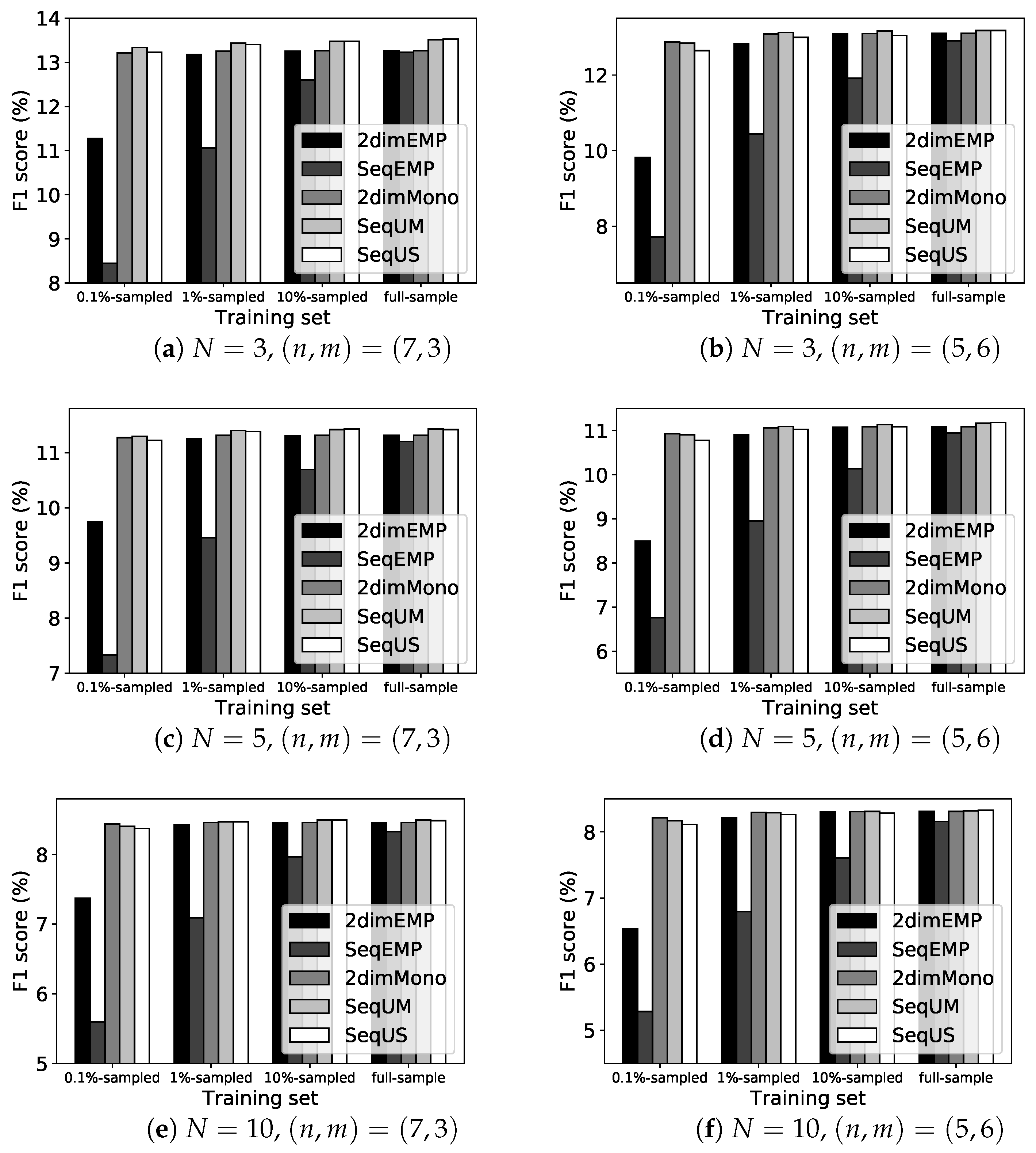
• We derive two types of PV sequence posets according to the recency and frequency of a user’s previous PVs. Experimental results show that the monotonicity constraints based on these posets greatly enhances the prediction performance of our PV sequence model.
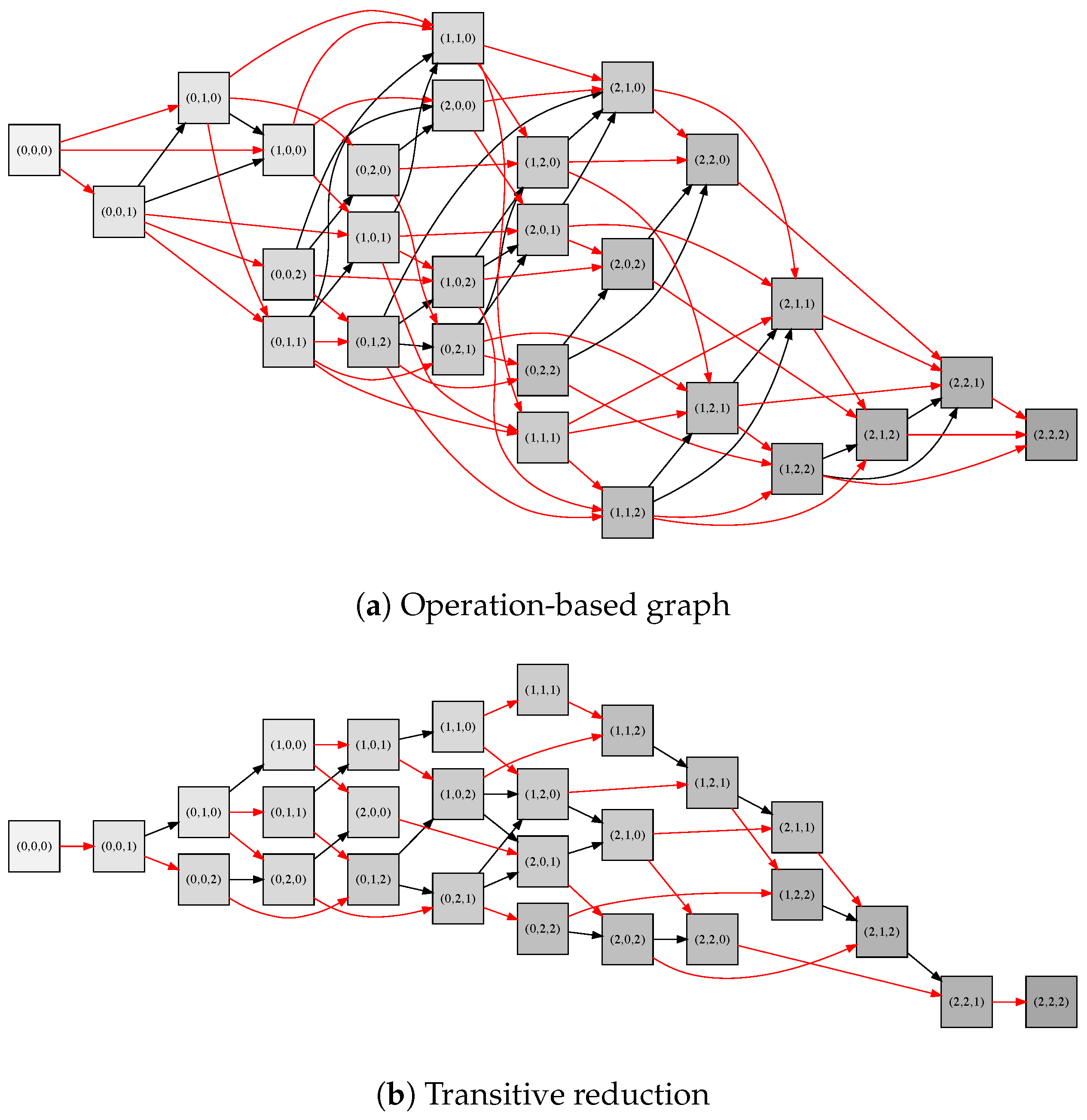
• We devise constructive algorithms for transitive reduction specific to these posets. The time complexity of our algorithms is much smaller than that of general-purpose algorithms. Experimental results reveal that transitive reduction improves efficiency in terms of both the computation time and memory usage of our PV sequence model.
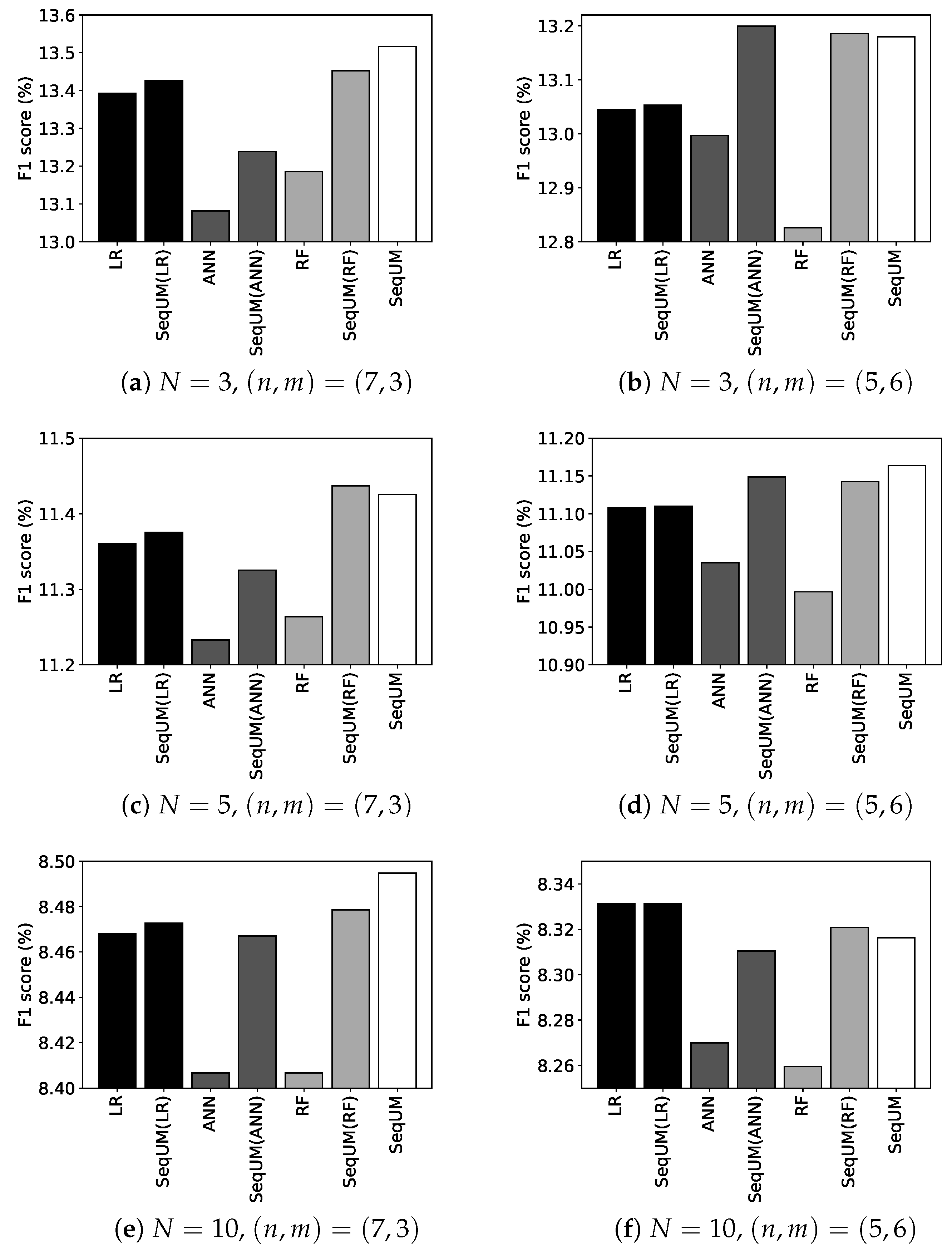
• We verify experimentally that higher prediction performance is achieved with our method than with the two-dimensional probability table and common machine learning methods, namely, logistic regression, artificial neural networks, and random forests.

The remainder of this paper is organized as follows. Section 2 provides a brief review of related work. Section 3 describes the two-dimensional probability table [11], and Section 4 presents our PV sequence model. Section 5 describes our constructive algorithms for transitive reduction. Section 6 evaluates the effectiveness of our method based on experimental results. Section 7 concludes with a brief summary of this work and a discussion of future research directions.

2. Related Work

This section briefly surveys methods for predicting online user behavior and discusses some related work on shape-restricted regression.

2.1. Prediction of Online User Behavior

A number of prior studies have aimed at predicting users’ purchase behavior on e-commerce websites [14]. Mainstream research has applied stochastic or statistical models for predicting purchase sessions [9,15,16,17,18,19,20], but these approaches do not consider which items users choose.

Various machine learning methods have been used to predict online item-choice behavior, including logistic regression [21,22], association rule mining [23], support vector machines [22,24], ensemble learning methods [25,26,27,28,29], and artificial neural networks [30,31,32]. Tailored statistical models have also been proposed. For instance, Moe [33] devised a two-stage multinomial logit model that separates the decision-making process into item views and purchase decisions. Yao et al. [34] proposed a joint framework consisting of user-level factor estimation and item-level factor aggregation based on the buyer decision process. Borges and Levener [35] used Markov chain models to estimate the probability of the next link choice of a user.

These prior studies effectively utilized clickstream data in various prediction methods and showed that the consideration of time-evolving user behavior is crucial for the precise prediction of online item-choice behavior. We therefore focused on user PV sequences to estimate item-choice probabilities on e-commerce websites.

On the other hand, various predictive features have been used for analyzing online user behavior; these include user demographics, item characteristics, transaction timestamps, accessing devices, touchpoints, and user locations [14]. Indeed, Nishimura et al. [12] demonstrated that the prediction performance can be improved by combining PV histories with item categories. To further upgrade the prediction performance, we aim at exploiting the detailed information contained in the PV history rather than developing a comprehensive model that integrates various predictive features. If successful, we can improve the prediction performance of comprehensive models through ensemble learning. Additionally, user PV histories are often easily accessible in practical situations, whereas detailed personal information can be unavailable due to a privacy issue.

Recently, deep learning methods have been actively studied to predict online user behavior especially in recommender systems; these include the multilayer perceptron, the autoencorder, convolutional/recurrent neural networks, and neural attention models [36]. In particular, graph neural networks [37,38] that operate on graph data have been used effectively because most of the information about users’ item-choice behavior has a graph structure. Sophisticated methods based on graph neural networks have been proposed for purchase prediction [39,40,41,42], and these can be considered as a top line on the prediction performance. In contrast, our method has a different advantage from such deep learning methods; it is a simple interpretable nonparametric model specialized in handling PV sequences based on properties indicated by the recency and frequency. Moreover, we evaluated the validity of our method by comparison with machine learning methods that have commonly been used in prior studies.

2.2. Shape-Restricted Regression

In many practical situations, prior information is known about the relationship between explanatory and response variables. For instance, utility functions can be assumed to be increasing and concave according to economic theory [43], and option pricing functions to be monotone and convex according to finance theory [44]. Shape-restricted regression fits a nonparametric function to a set of given observations under shape restrictions such as monotonicity, convexity, concavity, or unimodality [45,46,47,48].

Isotonic regression is the most common method for shape-restricted regression. In general, isotonic regression is the problem of estimating a real-valued monotone (non-decreasing or non-increasing) function with respect to a given partial order of observations [49]. Some regularization techniques [50,51] and estimation algorithms [49,52,53] have been proposed for isotonic regression.

One of the greatest advantages of shape-restricted regression is that it mitigates overfitting, thereby improving the prediction performance of regression models [54]. To utilize this advantage, Iwanaga et al. [11] devised a shape-restricted optimization model for estimating item-choice probabilities on e-commerce websites. Along similar lines, we propose a shape-restricted optimization model based on order relations of PV sequences to improve prediction performance.

3. Two-Dimensional Probability Table

This section briefly reviews the two-dimensional probability table proposed by Iwanaga et al. [11].

3.1. Empirical Probability Table

Table 1. Pageview history of six user–item pairs.

		#PVs				Choice
User	Item	1 April	2 April	3 April		4 April	$(\mathit{r},\mathit{f})$	$({\mathit{v}}_{\mathbf{1}},{\mathit{v}}_{\mathbf{2}},{\mathit{v}}_{\mathbf{3}})$
$u_1$	$i_2$	1	0	1		0	$(3,2)$	$(1,0,1)$
$u_1$	$i_4$	0	1	0		1	$(2,1)$	$(0,1,0)$
$u_2$	$i_1$	3	0	0		0	$(1,3)$	$(0,0,3)$
$u_2$	$i_3$	0	0	3		1	$(3,3)$	$(3,0,0)$
$u_2$	$i_4$	1	1	1		0	$(3,3)$	$(1,1,1)$
$u_3$	$i_2$	2	0	1		0	$(3,3)$	$(1,0,2)$

gives an example of a PV history for six user–item pairs. For instance, user $u_1$ viewed the page for item $i_2$ once on 1 and 3 April, respectively. We focus on user choices (e.g., revisit and purchase) on 4 April, which we call the base date. For instance, user $u_1$ chose item $i_4$ rather than item $i_2$ on the base date. We suppose for each user–item pair that recency and frequency are characterized by the last PV day and the total number of PVs, respectively. As shown in the table, the PV history can be summarized by the recency–frequency combination $(r,f)\in R\times F$, where R and F are index sets representing recency and frequency, respectively.

Let $n_{rf}$ be the number of user–item pairs having $(r,f)\in R\times F$, and set $q_{rf}$ be the number of choices occurring by user–item pairs that have $(r,f)\in R\times F$ on the base date. In the case of Table 1, the empirical probability table is calculated as

$$\begin{array}{cc}\hfill {\left({\widehat{x}}_{rf}:=\frac{q_{rf}}{n_{rf}}\right)}_{(r,f)\in R\times F}& \hfill =\left(\begin{array}{ccc}0/0& 0/0& 0/1\\ 1/1& 0/0& 0/0\\ 0/0& 0/1& 1/3\end{array}\right)\approx \left(\begin{array}{ccc}\hfill 0.00\hfill & \hfill 0.00\hfill & \hfill 0.00\hfill \\ \hfill 1.00\hfill & \hfill 0.00\hfill & \hfill 0.00\hfill \\ \hfill 0.00\hfill & \hfill 0.00\hfill & \hfill 0.33\hfill \end{array}\right),\hfill \end{array}$$

(1)

where, for reasons of expediency, ${\widehat{x}}_{rf}:=0$ for $(r,f)\in R\times F$ with $n_{rf}=0$.

3.2. Two-Dimensional Monotonicity Model

It is reasonable to assume that the recency and frequency of user–item pairs are positively associated with user item-choice probabilities. To estimate user item-choice probabilities $x_{rf}$ for all recency–frequency combinations $(r,f)\in R\times F$, the two-dimensional monotonicity model [11] minimizes the weighted sum of squared errors under monotonicity constraints with respect to recency and frequency.

$$\begin{array}{cc}\hfill \underset{{\left(x_{rf}\right)}_{(r,f)\in R\times F}}{\mathrm{minimize}}& \hfill \sum _{(r,f)\in R\times F}{n}_{rf}{(x_{rf}-{\widehat{x}}_{rf})}^2\hfill \end{array}$$

(2)

$$\begin{array}{cc}\hfill \mathrm{subject}\mathrm{to}& \hfill x_{rf}\le x_{r+1,f}((r,f)\in R\times F),\hfill \end{array}$$

(3)

$$\begin{array}{cc}\hfill & \hfill x_{rf}\le x_{r,f+1}((r,f)\in R\times F),\hfill \end{array}$$

(4)

$$\begin{array}{cc}\hfill & \hfill 0\le x_{rf}\le 1((r,f)\in R\times F).\hfill \end{array}$$

(5)

Note, however, that PV histories are often indistinguishable according to recency and frequency. A typical example is the set of user–item pairs $(u_2,i_3)$, $(u_2,i_4)$, and $(u_3,i_2)$ in Table 1; although their PV histories are actually different, they have the same value $(r,f)=(3,3)$ for recency–frequency combinations. As described in the next section, we exploit the PV sequence to distinguish between such PV histories.

4. PV Sequence Model

This section presents our shape-restricted optimization model for estimating item-choice probabilities from a user’s previous PV sequence.

4.1. PV Sequence

The PV sequence for each user–item pair represents a time series of the number of PVs, and is written as

$$\mathit{v}:=(v_1,v_2,\dots ,v_n),$$

where $v_j$ is the number of PVs j periods earlier for $j=1,2,\dots ,n$ (see Table 1). Note that sequence terms are arranged in reverse chronological order; thus, $v_j$ moves into the past as the index j increases.

Throughout the paper, we express sets of consecutive integers as

$$[m_1,m_2]:=\{m_1,m_1+1,\dots ,m_2\}\subseteq \mathbb{Z},$$

where $[m_1,m_2]=\varnothing$ when $m_1>m_2$. The set of possible PV sequences is defined as

$$\Gamma :={[0,m]}^n={\{0,1,\dots ,m\}}^n,$$

where m is the maximum number of PVs in each period, and n is the number of periods considered.

Our objective is to estimate item-choice probabilities $x_{\mathit{v}}$ for all PV sequences $\mathit{v}\in \Gamma$. However, the huge number of PV sequences makes it extremely difficult to accurately estimate such probabilities. In the case of $(n,m)=\left(\right|R|,|F\left|\right)=(5,6)$, for instance, the number of different PV sequences is ${(m+1)}^n=16,807$, whereas the number of recency–frequency combinations is only $\left|R\right|·\left|F\right|=30$. To avoid this difficulty, we effectively utilize monotonicity constraints on item-choice probabilities as in the optimization model (2)–(5). In the next section, we introduce three operations underlying the development of the monotonicity constraints.

4.2. Operations Based on Recency and Frequency

From the perspective of frequency, it is reasonable to assume that item-choice probability increases as the number of PVs in a particular period increases. To formulate this, we define the following operation:

Definition 1

($\mathtt{Up}$). On the domain

$${\mathcal{D}}_{\mathtt{U}}:=\{(\mathit{v},s)\in \Gamma \times [1,n]\mid v_s\le m-1\},$$

the function $\mathtt{Up}:{\mathcal{D}}_{\mathtt{U}}\to \Gamma$ is defined as

$$((\dots ,v_s,\dots ),s)\mapsto (\dots ,v_s+1,\dots ).$$

For instance, we have $\mathtt{Up}\left(\right(0,1,1),1)=(1,1,1)$, and $\mathtt{Up}\left(\right(1,1,1),2)=(1,2,1)$. Since this operation increases PV frequencies, the monotonicity constraint $x_{(0,1,1)}\le x_{(1,1,1)}\le x_{(1,2,1)}$ should be satisfied by item-choice probabilities.

From the perspective of recency, we assume that more-recent PVs have a larger effect on increasing item-choice probability. To formulate this, we consider the following operation for moving one PV from an old period to a new period:

Definition 2

($\mathtt{Move}$). On the domain

$$\begin{array}{c}\hfill {\mathcal{D}}_{\mathtt{M}}:=\{(\mathit{v},s,t)\in \Gamma \times [1,n]\times [1,n]\mid v_s\le m-1,v_t\ge 1,s<t\},\hfill \end{array}$$

the function $\mathtt{Move}:{\mathcal{D}}_{\mathtt{M}}\to \Gamma$ is defined as

$$((\dots ,v_s,\dots ,v_t,\dots ),s,t)\mapsto (\dots ,v_s+1,\dots ,v_t-1,\dots ).$$

For instance, we have $\mathtt{Move}\left(\right(1,1,1),2,3)=(1,2,0)$, and $\mathtt{Move}\left(\right(1,2,0),1,2)=(2,1,0)$. Because this operation increases the number of recent PVs, item-choice probabilities should satisfy the monotonicity constraint $x_{(1,1,1)}\le x_{(1,2,0)}\le x_{(2,1,0)}$.

The PV sequence $\mathit{v}=(1,1,1)$ represents a user’s continued interest in a certain item over three periods. In contrast, the PV sequence $\mathit{v}=(1,2,0)$ implies that a user’s interest decreased over the two most-recent periods. In this sense, the monotonicity constraint $x_{(1,1,1)}\le x_{(1,2,0)}$ may not be validated. Accordingly, we define the following alternative operation, which exchanges numbers of PVs to increase the number of recent PVs:

Definition 3

($\mathtt{Swap}$). On the domain

$${\mathcal{D}}_{\mathtt{S}}:=\{(\mathit{v},s,t)\in \Gamma \times [1,n]\times [1,n]\mid v_s<v_t,s<t\},$$

the function $\mathtt{Swap}:{\mathcal{D}}_{\mathtt{S}}\to \Gamma$ is defined as

$$((\dots ,v_s,\dots ,v_t,\dots ),s,t)\mapsto (\dots ,v_t,\dots ,v_s,\dots ).$$

We thus have $\mathtt{Swap}\left(\right(1,0,2),2,3)=(1,2,0)$ because $v_2<v_3$, and $\mathtt{Swap}\left(\right(1,2,0),1,2)=(2,1,0)$ because $v_1<v_2$. Since this operation increases the number of recent PVs, item-choice probabilities should satisfy the monotonicity constraint $x_{(1,0,2)}\le x_{(1,2,0)}\le x_{(2,1,0)}$. Note that the monotonicity constraint $x_{(1,1,1)}\le x_{(1,2,0)}$ is not implied by this operation.

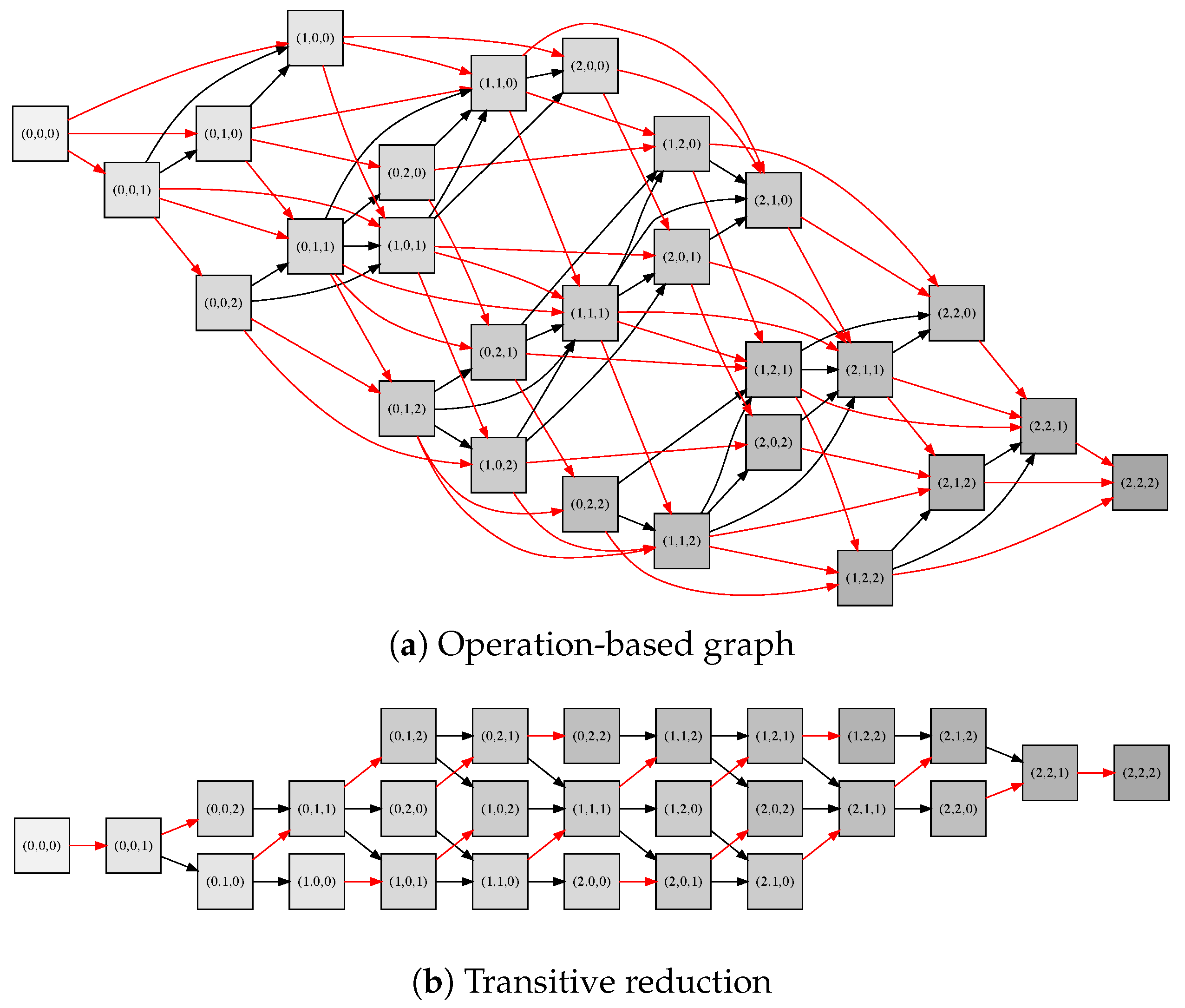
4.3. Partially Ordered Sets

Let $U\subseteq \Gamma$ be a subset of PV sequences. The image of each operation is then defined as

$$\begin{array}{cc}\hfill \mathtt{Up}\left(U\right)& \hfill =\{\mathtt{Up}(\mathit{u},s)\mid \mathit{u}\in U,(\mathit{u},s)\in {\mathcal{D}}_{\mathtt{U}}\},\hfill \\ \hfill \mathtt{Move}\left(U\right)& \hfill =\{\mathtt{Move}(\mathit{u},s,t)\mid \mathit{u}\in U,(\mathit{u},s,t)\in {\mathcal{D}}_{\mathtt{M}}\},\hfill \\ \hfill \mathtt{Swap}\left(U\right)& \hfill =\{\mathtt{Swap}(\mathit{u},s,t)\mid \mathit{u}\in U,(\mathit{u},s,t)\in {\mathcal{D}}_{\mathtt{S}}\}.\hfill \end{array}$$

We define $\mathtt{UM}\left(U\right):=\mathtt{Up}\left(U\right)\cup \mathtt{Move}\left(U\right)$ for $U\subseteq \Gamma$. The following definition states that the binary relation $\mathit{u}{\prec }_{\mathtt{UM}}\mathit{v}$ holds when $\mathit{u}$ can be transformed into $\mathit{v}$ by the repeated application of Up and Move:

Definition 4

(${⪯}_{\mathtt{UM}}$). Suppose $\mathit{u},\mathit{v}\in \Gamma$. We write $\mathit{u}{\prec }_{\mathtt{UM}}\mathit{v}$ if and only if there exists $k\ge 1$ such that

$$\mathit{v}\in {\mathtt{UM}}^k\left(\left\{\mathit{u}\right\}\right)=\underset{k\mathrm{compositions}}{\underbrace{\mathtt{UM}\circ \cdots \circ \mathtt{UM}\circ \mathtt{UM}}}\left(\left\{\mathit{u}\right\}\right).$$

We also write $\mathit{u}{⪯}_{\mathtt{UM}}\mathit{v}$ if $\mathit{u}{\prec }_{\mathtt{UM}}\mathit{v}$ or $\mathit{u}=\mathit{v}$.

Similarly, we define $\mathtt{US}\left(U\right):=\mathtt{Up}\left(U\right)\cup \mathtt{Swap}\left(U\right)$ for $U\subseteq \Gamma$. Then, the binary relation $\mathit{u}{\prec }_{\mathtt{US}}\mathit{v}$ holds when $\mathit{u}$ can be transformed into $\mathit{v}$ by the repeated application of Up and Swap.

Definition 5

(${⪯}_{\mathtt{US}}$). Suppose $\mathit{u},\mathit{v}\in \Gamma$. We write $\mathit{u}{\prec }_{\mathtt{US}}\mathit{v}$ if and only if there exists $k\ge 1$, such that

$$\mathit{v}\in {\mathtt{US}}^k\left(\left\{\mathit{u}\right\}\right)=\underset{k\mathrm{compositions}}{\underbrace{\mathtt{US}\circ \cdots \circ \mathtt{US}\circ \mathtt{US}}}\left(\left\{\mathit{u}\right\}\right).$$

We also write $\mathit{u}{⪯}_{\mathtt{US}}\mathit{v}$ if $\mathit{u}{\prec }_{\mathtt{US}}\mathit{v}$ or $\mathit{u}=\mathit{v}$.

To prove properties of these binary relations, we can use the lexicographic order, which is a well-known linear order [55]:

Definition 6

(${⪯}_{\mathtt{lex}}$). Suppose $\mathit{u},\mathit{v}\in \Gamma$. We write $\mathit{u}{\prec }_{\mathtt{lex}}\mathit{v}$ if and only if there exists $s\in [1,n]$, such that $u_s<v_s$ and $u_j=v_j$ for $j\in [1,s-1]$. We also write $\mathit{u}{⪯}_{\mathtt{lex}}\mathit{v}$ if $\mathit{u}{\prec }_{\mathtt{lex}}\mathit{v}$ or $\mathit{u}=\mathit{v}$.

Each application of Up, Move, and Swap makes a PV sequence greater in the lexicographic order. Therefore, we can obtain the following lemma:

Lemma 1.

Suppose $\mathit{u},\mathit{v}\in \Gamma$. If $\mathit{u}{⪯}_{\mathtt{UM}}\mathit{v}$ or $\mathit{u}{⪯}_{\mathtt{US}}\mathit{v}$, then $\mathit{u}{⪯}_{\mathtt{lex}}\mathit{v}$.

The following theorem states that a partial order of PV sequences is derived by operations Up and Move.

Theorem 1.

The pair $(\Gamma ,{⪯}_{\mathtt{UM}})$ is a poset.

Proof. 

From Definition 4, the relation ${⪯}_{\mathtt{UM}}$ is reflexive and transitive. Suppose $\mathit{u}{⪯}_{\mathtt{UM}}\mathit{v}$ and $\mathit{v}{⪯}_{\mathtt{UM}}\mathit{u}$. It follows from Lemma 1 that $\mathit{u}{⪯}_{\mathtt{lex}}\mathit{v}$ and $\mathit{v}{⪯}_{\mathtt{lex}}\mathit{u}$. Since the relation ${⪯}_{\mathtt{lex}}$ is antisymmetric, we have $\mathit{u}=\mathit{v}$, thus proving that the relation ${⪯}_{\mathtt{UM}}$ is also antisymmetric.    □

We can similarly prove the following theorem for operations Up and Swap:

Theorem 2.

The pair $(\Gamma ,{⪯}_{\mathtt{US}})$ is a poset.

4.4. Shape-Restricted Optimization Model

Let $n_{\mathit{v}}$ be the number of user–item pairs that have the PV sequence $\mathit{v}\in \Gamma$. Moreover, $q_{\mathit{v}}$ is the number of choices arising from user–item pairs having $\mathit{v}\in \Gamma$ on the base date. Similarly to Equation (1), we can calculate empirical item-choice probabilities as

$$\begin{array}{c}\hfill {\widehat{x}}_{\mathit{v}}:=\frac{q_{\mathit{v}}}{n_{\mathit{v}}}(\mathit{v}\in \Gamma ).\end{array}$$

(6)

Our shape-restricted optimization model minimizes the weighted sum of squared errors subject to the monotonicity constraint:

$$\begin{array}{cc}\hfill \underset{{\left(x_{\mathit{v}}\right)}_{\mathit{v}\in \Gamma }}{\mathrm{minimize}}& \hfill \sum _{\mathit{v}\in \Gamma }{n}_{\mathit{v}}{(x_{\mathit{v}}-{\widehat{x}}_{\mathit{v}})}^2\hfill \end{array}$$

(7)

$$\begin{array}{cc}\hfill \mathrm{subject}\mathrm{to}& \hfill x_{\mathit{u}}\le x_{\mathit{v}}(\mathit{u},\mathit{v}\in \Gamma \mathrm{with}\mathit{u}\prec \mathit{v}),\hfill \end{array}$$

(8)

$$\begin{array}{cc}\hfill & \hfill 0\le x_{\mathit{v}}\le 1(\mathit{v}\in \Gamma ),\hfill \end{array}$$

(9)

where $\mathit{u}\prec \mathit{v}$ in Equation (8) is defined by one of the partial orders ${\prec }_{\mathtt{UM}}$ or ${\prec }_{\mathtt{US}}$.

The monotonicity constraint (8) enhances the estimation accuracy of item-choice probabilities. In addition, our shape-restricted optimization model can be used in a post-processing step to improve the prediction performance of other machine learning methods. Specifically, we first compute item-choice probabilities using a machine learning method and then substitute the computed values into ${\left({\widehat{x}}_{\mathit{v}}\right)}_{\mathit{v}\in \Gamma }$ to solve the optimization model (7)–(9). Consequently, we can obtain item-choice probabilities corrected by the monotonicity constraint (8). Section 6.4 illustrates the usefulness of this approach.

However, since $|\Gamma |={(m+1)}^n$, it follows that the number of constraints in Equation (8) is $\mathcal{O}\left({(m+1)}^{2n}\right)$, which can be extremely large. When $(n,m)=(5,6)$, for instance, we have ${(m+1)}^{2n}=282,475,249$. The next section describes how we mitigate this difficulty by removing redundant constraints in Equation (8).

5. Algorithms for Transitive Reduction

This section describes our constructive algorithms for transitive reduction to decrease the problem size in our shape-restricted optimization model.

5.1. Transitive Reduction

A poset $(\Gamma ,⪯)$ can be represented by a directed graph $(\Gamma ,E)$, where $\Gamma$ and $E\subseteq \Gamma \times \Gamma$ are sets of nodes and directed edges, respectively. Each directed edge $(\mathit{u},\mathit{v})\in E$ in this graph corresponds to the order relation $\mathit{u}\prec \mathit{v}$, so the number of directed edges coincides with the number of constraints in Equation (8).

Figure 1 and Figure 2 show directed graph representations of posets $(\Gamma ,{⪯}_{\mathtt{UM}})$ and $(\Gamma ,{⪯}_{\mathtt{US}})$, respectively. Each edge in Figure 1a and Figure 2a corresponds to one of the operations Up, Move, or Swap. Edge $(\mathit{u},\mathit{v})$ is red if $\mathit{v}\in \mathtt{Up}\left(\right\{\mathit{u}\left\}\right)$ and black if $\mathit{v}\in \mathtt{Move}\left(\right\{\mathit{u}\left\}\right)$ or $\mathit{v}\in \mathtt{Swap}\left(\right\{\mathit{u}\left\}\right)$. The directed graphs in Figure 1a and Figure 2a can be easily created.

Suppose there are three edges $(\mathit{u},\mathit{w}),(\mathit{w},\mathit{v}),(\mathit{u},\mathit{v})\in E$. In this case, edge $(\mathit{u},\mathit{v})$ is implied by the other edges due to the transitivity of partial order

$$\langle \mathit{u}\prec \mathit{w},\mathit{w}\prec \mathit{v}\rangle \Rightarrow \mathit{u}\prec \mathit{v},$$

or, equivalently,

$$\langle x_{\mathit{u}}\le x_{\mathit{w}},x_{\mathit{w}}\le x_{\mathit{v}}\rangle \Rightarrow x_{\mathit{u}}\le x_{\mathit{v}}.$$

As a result, edge $(\mathit{u},\mathit{v})$ is redundant and can be removed from the directed graph.

A transitive reduction, also known as a Hasse diagram, of a directed graph $(\Gamma ,E)$ is its subgraph $(\Gamma ,E^{*})$ such that all redundant edges are removed using the transitivity of partial order [13]. Figure 1b and Figure 2b show transitive reductions of the directed graphs shown in Figure 1a and Figure 2a, respectively. By computing transitive reductions, the number of edges is reduced from 90 to 42 in Figure 1, and from 81 to 46 in Figure 2. This transitive reduction is known to be unique [13].

5.2. General-Purpose Algorithms

The transitive reduction $(\Gamma ,E^{*})$ is characterized by the following lemma [55]:

Lemma 2.

Suppose $(\mathit{u},\mathit{v})\in \Gamma \times \Gamma$. Then, $(\mathit{u},\mathit{v})\in E^{*}$ holds if and only if both of the following conditions are fulfilled:

(C1)

$\mathit{u}\prec \mathit{v}$, and

(C2)

if $\mathit{w}\in \Gamma$ satisfies $\mathit{u}⪯\mathit{w}⪯\mathit{v}$, then $\mathit{w}\in \{\mathit{u},\mathit{v}\}$.

The basic strategy in general-purpose algorithms for transitive reduction involves the following steps:

Step 1:

An exhaustive directed graph $(\Gamma ,E)$ is generated from a given poset $(\Gamma ,⪯)$.

Step 2:

The transitive reduction $(\Gamma ,E^{*})$ is computed from the directed graph $(\Gamma ,E)$ using Lemma 2.

Various algorithms for speeding up the computation in Step 2 have been proposed. Recall that $|\Gamma |={(m+1)}^n$ in our situation. Warshall’s algorithm [56] has time complexity $\mathcal{O}\left({(m+1)}^{3n}\right)$ for completing Step 2 [55]. By using a sophisticated algorithm for fast matrix multiplication, this time complexity can be reduced to $\mathcal{O}\left({(m+1)}^{2.3729n}\right)$ [57].

However, such general-purpose algorithms are clearly inefficient, especially when n is very large, and Step 1 requires a huge number of computations. To resolve this difficulty, we devised specialized algorithms for directly constructing a transitive reduction.

5.3. Constructive Algorithms

Let $(\Gamma ,E_{\mathtt{UM}}^{*})$ be a transitive reduction of a directed graph $(\Gamma ,E_{\mathtt{UM}})$ representing the poset $(\Gamma ,{⪯}_{\mathtt{UM}})$. Then, the transitive reduction can be characterized by the following theorem:

Theorem 3.

Suppose $(\mathit{u},\mathit{v})\in \Gamma \times \Gamma$. Then, $(\mathit{u},\mathit{v})\in E_{\mathtt{UM}}^{*}$ holds if and only if any one of the following conditions is fulfilled:

(UM1)

$\mathit{v}=\mathtt{Up}(\mathit{u},n)$, or

(UM2)

there exists $s\in [1,n]$ such that $\mathit{v}=\mathtt{Move}(\mathit{u},s,s+1)$.

Proof. 

See Appendix A.1.    □

Theorem 3 provides a constructive algorithm that directly computes the transitive reduction $(\Gamma ,E_{\mathtt{UM}}^{*})$ without generating an exhaustive directed graph $(\Gamma ,E)$. Our algorithm is based on the breadth-first search [58]. Specifically, we start with a node list $L=\left\{\right(0,0,\dots ,0\left)\right\}\subseteq \Gamma$. At each iteration of the algorithm, we choose $\mathit{u}\in L$, enumerate $\mathit{v}\in \Gamma$ such that $(\mathit{u},\mathit{v})\in E_{\mathtt{UM}}^{*}$, and add these nodes to L.

Table 2. Process of enumerating $\mathit{v}\in \Gamma$ such that $(\mathit{u},\mathit{v})\in E_{\mathtt{UM}}^{*}$.

u	Operation	v	(UM1)	(UM2)
$(0,2,1)$	$\mathtt{Up}(\mathit{u},1)$	$(1,2,1)$	unsatisfied	—
	$\mathtt{Up}(\mathit{u},3)$	$(0,2,2)$	satisfied	—
	$\mathtt{Move}(\mathit{u},1,2)$	$(1,1,1)$	—	satisfied
	$\mathtt{Move}(\mathit{u},1,3)$	$(1,2,0)$	—	unsatisfied

shows this enumeration process for $\mathit{u}=(0,2,1)$ with $(n,m)=(3,2)$. The operations Up and Move generate $\mathit{v}\in \left\{\right(1,2,1),(0,2,2),(1,1,1),(1,2,0\left)\right\}$, which amounts to searching edges $(\mathit{u},\mathit{v})$ in Figure 1a. We next check whether each $\mathit{v}$ satisfies conditions (UM1) or (UM2) in Theorem 3. As shown in Table 2, we choose $\mathit{v}\in \left\{\right(0,2,2),(1,1,1\left)\right\}$ and add them to list L; this amounts to enumerating edges $(\mathit{u},\mathit{v})$ in Figure 1b.

Appendix B.1 presents a pseudocode for our constructive algorithm (Algorithm A1). Recalling the time complexity analysis of the breadth-first search [58], one readily sees that the time complexity of Algorithm A1 is $\mathcal{O}\left(n{(m+1)}^n\right)$, which is much smaller than $\mathcal{O}\left({(m+1)}^{2.3729n}\right)$, as achieved by the general-purpose algorithm [57], especially when n is very large.

Next, we focus on the transitive reduction $(\Gamma ,E_{\mathtt{US}}^{*})$ of a directed graph $(\Gamma ,E_{\mathtt{US}})$ representing the poset $(\Gamma ,{⪯}_{\mathtt{US}})$. The transitive reduction can then be characterized by the following theorem:

Theorem 4.

Suppose $(\mathit{u},\mathit{v})\in \Gamma \times \Gamma$. Then, $(\mathit{u},\mathit{v})\in E_{\mathtt{US}}^{*}$ holds if and only if any one of the following conditions is fulfilled:

(US1)

there exists $s\in [1,n]$ such that $\mathit{v}=\mathtt{Up}(\mathit{u},s)$ and $u_j\notin \{u_s,u_s+1\}$ for all $j\in [s+1,n]$, or

(US2)

there exists $(s,t)\in [1,n]\times [1,n]$ such that $\mathit{v}=\mathtt{Swap}(\mathit{u},s,t)$ and $u_j\notin [u_s,u_t]$ for all $j\in [s+1,t-1]$.

Proof. 

See Appendix A.2.    □

Theorem 4 also gives a constructive algorithm for computing the transitive reduction $(\Gamma ,E_{\mathtt{US}}^{*})$. Let us again consider $\mathit{u}=(0,2,1)$ as an example with $(n,m)=(3,2)$. As shown in

Table 3. Process of enumerating $\mathit{v}\in \Gamma$ such that $(\mathit{u},\mathit{v})\in E_{\mathtt{US}}^{*}$.

u	Operation	v	(US1)	(US2)
$(0,2,1)$	$\mathtt{Up}(\mathit{u},1)$	$(1,2,1)$	unsatisfied	—
	$\mathtt{Up}(\mathit{u},3)$	$(0,2,2)$	satisfied	—
	$\mathtt{Swap}(\mathit{u},1,2)$	$(2,0,1)$	—	satisfied
	$\mathtt{Swap}(\mathit{u},1,3)$	$(1,2,0)$	—	satisfied

, operations Up and Swap generate $\mathit{v}\in \left\{\right(1,2,1),(0,2,2),(2,0,1),(1,2,0\left)\right\}$, and we choose $\mathit{v}\in \left\{\right(0,2,2),(2,0,1),(1,2,0\left)\right\}$ (see also Figure 2a,b).

Appendix B.2 presents the pseudocode for our constructive algorithm (Algorithm A2). Its time complexity is estimated to be $\mathcal{O}\left(n^2{(m+1)}^n\right)$, which is larger than that of Algorithm A1 but much smaller than that of the general-purpose algorithm [57], especially when n is very large.

6. Experiments

The experimental results reported in this section evaluate the effectiveness of our method for estimating item-choice probabilities. We consider the task of predicting the items that a particular user will view again from those which the user has viewed in the past. The performance evaluation methodology is explained in detail in Section 6.2.

We used real-world clickstream data collected from a Chinese e-commerce website, Tmall (https://tianchi.aliyun.com/dataset/, accessed on 21 August 2023). We used a dataset (https://www.dropbox.com/sh/dbzmtq4zhzbj5o9/AACldzQWbw-igKjcPTBI6ZPAa?dl=0, accessed on 21 August 2023) preprocessed by Ludewig and Jannach [59]. Each record corresponds to one PV and contains information such as user ID, item ID, and a timestamp. The dataset includes 28,316,459 unique user–item pairs composed from 422,282 users and 624,221 items.

6.1. Methods for Comparison

We compared the performance of the methods listed in

Table 4. Methods for comparison.

Abbreviation	Method
2dimEmp	Empirical probability table (1) [11]
2dimMono	Two-dimensional monotonicity model (2)–(5) [11]
SeqEmp	Empirical probabilities (6) for PV sequences
SeqUM	Our PV sequence model (7)–(9) using $(\Gamma ,{⪯}_{\mathtt{UM}})$
SeqUS	Our PV sequence model (7)–(9) using $(\Gamma ,{⪯}_{\mathtt{US}})$
LR	$L_2$-regularized logistic regression
ANN	Artificial neural networks for regression using
	one fully-connected hidden layer of 100 units
RF	Random forest of regression trees

. All computations were performed on an Apple MacBook Pro computer (Apple Inc., Cupertino, CA, USA) with an Intel Core i7-5557U CPU (3.10 GHz) (Intel Corporation, Santa Clara, CA, USA) and 16 GB of memory.

The optimization models (2)–(5) and (7)–(9) were solved using OSQP (https://osqp.org/docs/index.html, accessed on 21 August 2023) [60], a numerical optimization package for solving convex quadratic optimization problems. As in Table 1, daily-PV sequences were calculated for each user–item pair, where m is the maximum number of daily PVs and n is the number of terms (past days) in the PV sequence. In this process, all PVs from more than n days earlier were added to the number of PVs n days earlier, and numbers of daily PVs exceeding m were rounded down to m. Similarly, the recency–frequency combinations $(r,f)\in R\times F$ were calculated using daily PVs as in Table 1, where $\left(\right|R|,|F\left|\right)=(n,m)$.

Other machine learning methods (LR, ANN, and RF) were respectively implemented using the LogisticRegressionCV, MLPRegressor, and RandomForestRegressor functions in scikit-learn, a Python library of machine learning tools. We tuned the following hyperparameters through three-fold cross-validation according to the parameter settings in a benchmark study [61]: Activation functions, solvers, and learning rate schedules for ANN; and the number of trees, the minimum weighted fraction at a leaf node, and the number of features considered at each split for RF. We used default values for the other hyperparameters. These machine learning methods employed the PV sequence $(v_1,v_2,\dots ,v_n)$ as n input variables for computing item-choice probabilities. We standardized each input variable and performed undersampling to improve prediction performance.

6.2. Performance Evaluation Methodology

There are five pairs of training and validation sets of clickstream data in the preprocessed dataset [59]. As shown in

Table 5. Training and validation periods.

	Training
Pair ID	Start	End	Validation
1	21 May 2015	18 August 2015	19 August 2015
2	31 May 2015	28 August 2015	29 August 2015
3	10 June 2015	7 September 2015	8 September 2015
4	20 June 2015	17 September 2015	18 September 2015
5	30 June 2015	27 September 2015	28 September 2015

, each training period is 90 days, and the next day is the validation period. The first four pairs of training and validation sets, which we call the training set, were used for model estimation, and the fifth pair was used for performance evaluation. To examine how sample size affects prediction performance, we prepared small-sample training sets by randomly choosing user–item pairs from the original training set. Here, the sampling rates are 0.1%, 1%, and 10%, and the original training set is referred to as the full sample. Note that the results were averaged over 10 trials for the sampled training sets.

We considered the top-N selection task to evaluate prediction performance. Specifically, we focused on items that were viewed by a particular user during a training period. From among these items, we selected $I_{\mathrm{sel}}$, a set of top-N items for the user according to estimated item-choice probabilities. The most-recently viewed items were selected when two or more items had the same choice probability. Let $I_{\mathrm{view}}$ be the set of items viewed by the user in the validation period. Then, the F1 score is defined by the harmonic average of $Recall:=|I_{\mathrm{sel}}\cap I_{\mathrm{view}}|/|I_{\mathrm{view}}|$ and $Precision:=|I_{\mathrm{sel}}\cap I_{\mathrm{view}}|/|I_{\mathrm{sel}}|$ as

$$\mathrm{F}1\mathrm{score}:=\frac{2·\mathrm{Recall}·\mathrm{Precision}}{\mathrm{Recall}+\mathrm{Precision}}.$$

In the following sections, we examine F1 scores averaged over all users. The percentage of user–item pairs leading to item choices is only 0.16%.

6.3. Effects of the Transitive Reduction

We generated constraints in Equation (8) based on the following three directed graphs:

Case 1 (Enumeration):

All edges $(\mathit{u},\mathit{v})$ satisfying $\mathit{u}\prec \mathit{v}$ were enumerated.

Case 2 (Operation):

Edges corresponding to operations Up, Move, and Swap were generated as in Figure 1a and Figure 2a.

Case 3 (Reduction):

Transitive reduction was computed using our algorithms as in Figure 1b and Figure 2b.

Table 6. Problem size of our PV sequence model (7)–(9).

			#Cons in Equation (8)
			Enumeration			Operation			Reduction
$\mathit{n}$	$\mathit{m}$	#Vars	SeqUM	SeqUS		SeqUM	SeqUS		SeqUM	SeqUS
5	1	32	430	430		160	160		48	48
5	2	243	21,383	17,945		1890	1620		594	634
5	3	1024	346,374	255,260		9600	7680		3072	3546
5	4	3125	3,045,422	2,038,236		32,500	25,000		10,500	12,898
5	5	7776	18,136,645	11,282,058		86,400	64,800		28,080	36,174
5	6	16,807	82,390,140	48,407,475		195,510	144,060		63,798	85,272
1	6	7	21	21		6	6		6	6
2	6	49	1001	861		120	105		78	93
3	6	343	42,903	32,067		1638	1323		798	1018
4	6	2401	1,860,622	1,224,030		18,816	14,406		7350	9675
5	6	16,807	82,390,140	48,407,475		195,510	144,060		63,798	85,272

shows the problem size of our PV sequence model (7)–(9) for some $(n,m)$ settings of the PV sequence. Here, the “#Vars” column shows the number of decision variables (i.e., ${(m+1)}^n$), and the subsequent columns show the number of constraints in Equation (8) for the three cases mentioned above.

The number of constraints grew rapidly as n and m increased in the enumeration case. In contrast, the number of constraints was always kept smallest by the transitive reduction among the three cases. When $(n,m)=(5,6)$, for instance, transitive reductions reduced the number of constraints in the operation case to 63,798/195,510 $\approx 32.6\%$ for SeqUM and 85,272/144,060 $\approx 59.2\%$ for SeqUS.

The number of constraints was larger for SeqUM than for SeqUS in the enumeration and operation cases. In contrast, the number of constraints was often smaller for SeqUM than for SeqUS in the reduction case. Thus, the transitive reduction had a greater impact on SeqUM than on SeqUS in terms of the number of constraints.

Table 7. Computation times for our PV sequence model (7)–(9).

			Time [s]
			Enumeration			Operation			Reduction
$\mathit{n}$	$\mathit{m}$	#Vars	SeqUM	SeqUS		SeqUM	SeqUS		SeqUM	SeqUS
5	1	32	0.00	0.01		0.00	0.00		0.00	0.00
5	2	243	2.32	1.66		0.09	0.07		0.03	0.02
5	3	1024	558.22	64.35		3.41	0.71		0.13	0.26
5	4	3125	OM	OM		24.07	13.86		1.72	5.80
5	5	7776	OM	OM		180.53	67.34		9.71	36.94
5	6	16,807	OM	OM		906.76	522.84		86.02	286.30
1	6	7	0.00	0.00		0.00	0.00		0.00	0.00
2	6	49	0.03	0.01		0.01	0.00		0.00	0.00
3	6	343	12.80	1.68		0.20	0.03		0.05	0.02
4	6	2401	OM	OM		8.07	4.09		2.12	2.87
5	6	16,807	OM	OM		906.76	522.84		86.02	286.30

lists the computation times required for solving the optimization problem (7)–(9) for some $(n,m)$ settings of the PV sequence. Here, “OM” indicates that computation was aborted due to a lack of memory. The enumeration case often caused out-of-memory errors because of the huge number of constraints (see Table 6), but the operation and reduction cases completed the computations for all $(n,m)$ settings for the PV sequence. Moreover, the transitive reduction made computations faster. A notable example is SeqUM with $(n,m)=(5,6)$, for which the computation time in the reduction case (86.02 s) was only one-tenth of that in the operation case (906.76 s). These results demonstrate that transitive reduction improves efficiency in terms of both computation time and memory usage.

Table 8. Computational performance of our PV sequence model (7)–(9).

			#Cons in Equation (8)			Time [s]			F1 Score [%], $\mathit{N}=3$
$\mathit{n}$	$\mathit{m}$	#Vars	SeqUM	SeqUS		SeqUM	SeqUS		SeqEmp	SeqUM	SeqUS
3	30	29,791	84,630	118,850		86.72	241.46		12.25	12.40	12.40
4	12	28,561	99,372	142,800		198.82	539.76		12.68	12.93	12.95
5	6	16,807	63,798	85,272		86.02	286.30		12.90	13.18	13.18
6	4	15,625	62,500	76,506		62.92	209.67		13.14	13.49	13.48
7	3	16,384	67,584	76,818		96.08	254.31		13.23	13.52	13.53
8	2	6561	24,786	25,879		19.35	17.22		13.11	13.37	13.35
9	2	19,683	83,106	86,386		244.15	256.42		13.07	13.40	13.37

shows the computational performance of our optimization model (7)–(9) for some $(n,m)$ settings of PV sequences. Here, for each $n\in \{3,4\dots ,9\}$, the largest m was chosen such that the computation finished within 30 min. Both SeqUM and SeqUS always delivered higher F1 scores than SeqEmp did. This indicates that our monotonicity constraint (8) works well for improving prediction performance. The F1 scores provided by SeqUM and SeqUS were very similar and were the largest with $(n,m)=(7,3)$. In light of these results, we use the setting $(n,m)\in \left\{\right(7,3),(5,6\left)\right\}$ in the following sections.

6.4. Prediction Performance of Our PV Sequence Model

Figure 3 shows F1 scores of the two-dimensional probability table and our PV sequence model using the sampled training sets, where the number of selected items is $N\in \{3,5,10\}$, and the setting of the PV sequence is $(n,m)\in \left\{\right(7,3),(5,6\left)\right\}$.

When the full-sample training set was used, SeqUM and SeqUS always delivered a better prediction performance than the other methods did. When the 1%- and 10%-sampled training sets were used, the prediction performance of SeqUS decreased slightly, whereas SeqUM still performed best among all the methods. When the 0.1%-sampled training set was used, 2dimMono always performed better than SeqUS did, and 2dimMono also had the best prediction performance in the case of $(n,m)=(5,6)$. These results suggest that our PV sequence model performs very well, especially when the sample size is sufficiently large. The prediction performance of SeqEmp deteriorated rapidly as the sampling rate decreased, and this performance was always much worse than that of 2dimEmp. Meanwhile, SeqUM and SeqUS maintained high prediction performance even when the 0.1%-sampled training set was used. This suggests that the monotonicity constraint (8) in our PV sequence model is more effective than the monotonicity constraints (3) and (4) in the two-dimensional monotonicity model.

Figure 4 shows F1 scores for the machine learning methods (LR, ANN, and RF) and our PV sequence model (SeqUM) using the full-sample training set, where the number of selected items is $N\in \{3,5,10\}$, and the PV sequence setting is $(n,m)\in \left\{\right(7,3),(5,6\left)\right\}$. Note that in this figure, SeqUM(*) represents the optimization model (7)–(9), where the item-choice probabilities computed by each machine learning method were substituted into ${\left({\widehat{x}}_{\mathit{v}}\right)}_{\mathit{v}\in \Gamma }$ (see Section 4.4).

Prediction performance was better for SeqUM than for all the machine learning methods, except in the case of Figure 4f, where LR showed better prediction performance. Moreover, SeqUM(*) improved the prediction performance of the machine leaning methods, particularly for ANN and RF. This suggests that our monotonicity constraint (8) is also very helpful in correcting prediction values from other machine learning methods.

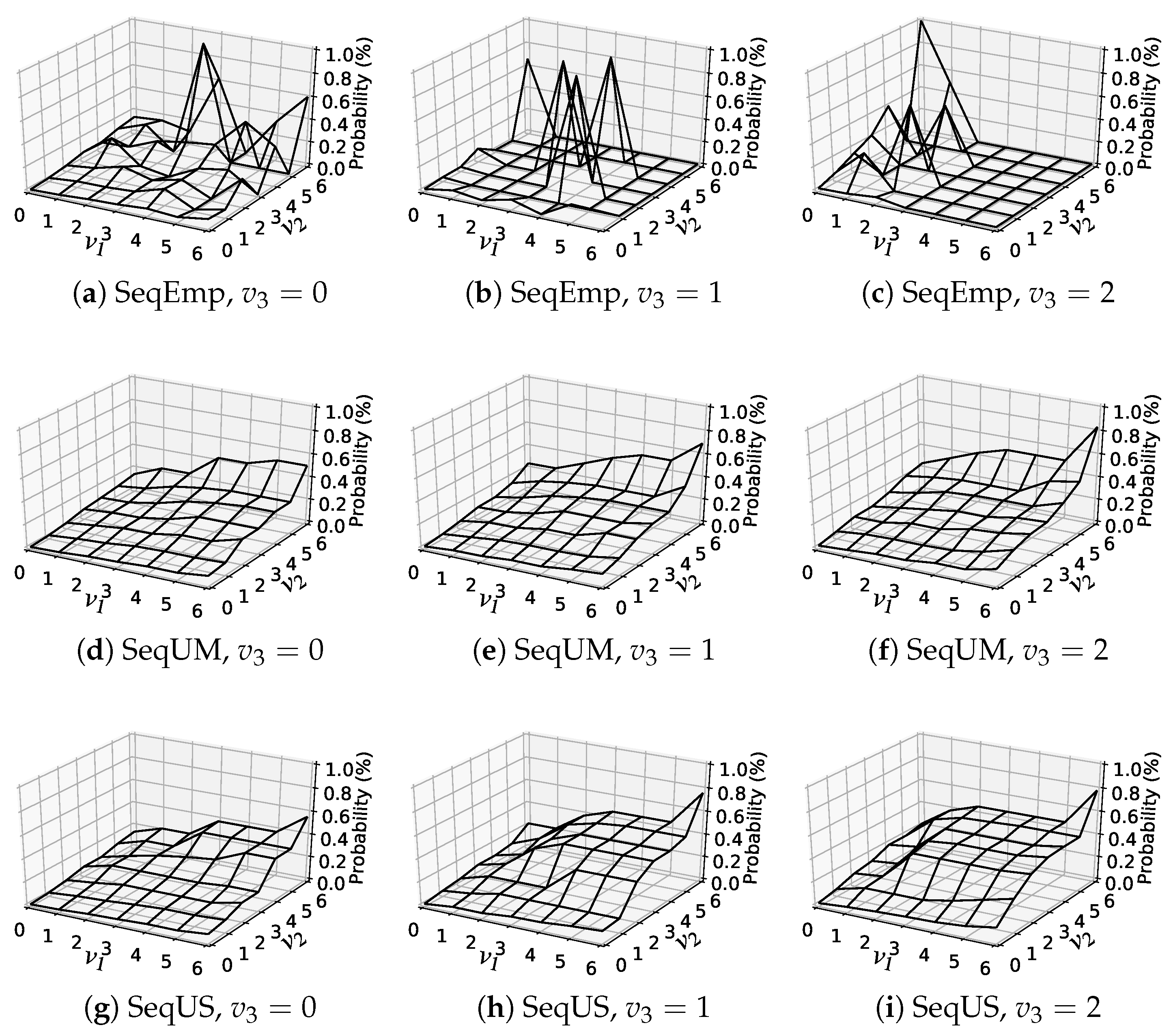
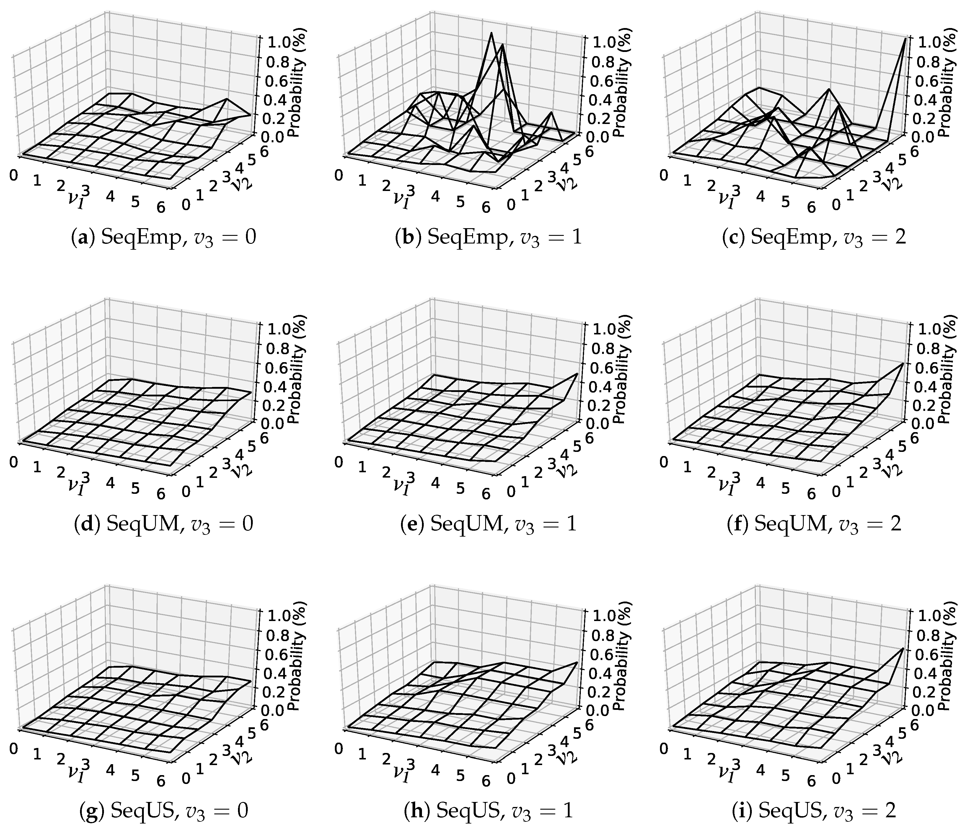
6.5. Analysis of Estimated Item-Choice Probabilities

Figure 5 shows item-choice probabilities estimated by our PV sequence model using the full-sample training set, where the PV sequence setting is $(n,m)=(5,6)$. Here, we focus on PV sequences in the form $\mathit{v}=(v_1,v_2,v_3,0,0)\in \Gamma$ and depict estimates of item-choice probabilities on $(v_1,v_2)\in [0,m]\times [0,m]$ for each $v_3\in \{0,1,2\}$. Note also that the number of associated user–item pairs decreased as the value of $v_3$ increased.

Because SeqEmp does not consider the monotonicity constraint (8), item-choice probabilities estimated by SeqEmp have irregular shapes for $v_3\in \{1,2\}$. In contrast, item-choice probabilities estimated with the monotonicity constraint (8) are relatively smooth. Because of the Up operation, item-choice probabilities estimated by SeqUM and SeqUS increase as $(v_1,v_2)$ moves from $(0,0)$ to $(6,6)$. Because of the Move operation, item-choice probabilities estimated by SeqUM also increase as $(v_1,v_2)$ moves from $(0,6)$ to $(6,0)$. item-choice probabilities estimated by SeqUS are relatively high, at around $(v_1,v_2)=(3,3)$. This highlights the difference in the monotonicity constraint (8) between posets $(\Gamma ,{⪯}_{\mathtt{UM}})$ and $(\Gamma ,{⪯}_{\mathtt{US}})$.

Figure 6 shows item-choice probabilities estimated by our PV sequence model using the 10%-sampled training set, where the PV sequence setting is $(n,m)=(5,6)$. Since the sample size was reduced in this case, item-choice probabilities estimated by SeqEmp are highly unstable. In particular, item-choice probabilities were estimated to be zero for all $(v_1,v_2)$ with $v_1\ge 3$ in Figure 6c, but this is unreasonable from the perspective of frequency. In contrast, SeqUM and SeqUS estimated item-choice probabilities that increase monotonically with respect to $(v_1,v_2)$.

7. Conclusions

We presented a shape-restricted optimization model for estimating item-choice probabilities on an e-commerce website. Our monotonicity constraints based on tailored order relations could better estimate item-choice probabilities for all possible PV sequences. To improve the computational efficiency of our optimization model, we devised constructive algorithms for transitive reduction that remove all redundant constraints from the optimization model.

We assessed the effectiveness of our method through experiments using real-world clickstream data. Experimental results demonstrated that transitive reduction enhanced the efficiency of our optimization model in terms of both computation time and memory usage. In addition, our method delivered a better prediction performance than did the two-dimensional monotonicity model [11] and common machine learning methods. Our method was also helpful in correcting prediction values computed by other machine learning methods.

This study made three main contributions. First, we derived two types of posets by exploiting the properties of recency and frequency of a user’s previous PVs. These posets allow us to place appropriate monotonicity constraints on item-choice probabilities. Next, we developed algorithms for the transitive reduction of our posets. These algorithms are more efficient than general-purpose algorithms in terms of time complexity for transitive reduction. Finally, our method further expanded the potential of shape-restricted regression for predicting user behavior on e-commerce websites.

Once the optimization model for estimating item-choice probabilities has been solved, the obtained results can easily be put into practical use on e-commerce websites. Accurate estimates of item-choice probabilities will be useful for customizing sales promotions according to the needs of a particular user. In addition, our method can estimate user preferences from clickstream data, therefore aiding in the creation of high-quality user–item rating matrices for recommendation algorithms [6].

In future studies, we will develop new posets that further improve the prediction performance of our PV sequence model. Another direction of future research will be to incorporate user–item heterogeneity into our optimization model, as in the case of latent-class modeling with a two-dimensional probability table [12]. It is also important to compare the prediction performance of our method with that of topline graph neural networks [37,38].

References

1. Turban, E.; Outland, J.; King, D.; Lee, J.K.; Liang, T.P.; Turban, D.C. Electronic Commerce 2018: A Managerial and Social Networks Perspective; Springer: Cham, Switzerland, 2017. [Google Scholar]
2. Kannan, P.; Li, H. Digital marketing: A framework, review and research agenda. Int. J. Res. Mark. 2017, 34, 22–45. [Google Scholar] [CrossRef]
3. Ngai, E.W.; Xiu, L.; Chau, D.C. Application of data mining techniques in customer relationship management: A literature review and classification. Expert Syst. Appl. 2009, 36, 2592–2602. [Google Scholar] [CrossRef]
4. Huang, T.; Van Mieghem, J.A. Clickstream data and inventory management: Model and empirical analysis. Prod. Oper. Manag. 2014, 23, 333–347. [Google Scholar] [CrossRef]
5. Aggarwal, C.C. Recommender Systems; Springer: Cham, Switzerland, 2016; Volume 1. [Google Scholar]
6. Iwanaga, J.; Nishimura, N.; Sukegawa, N.; Takano, Y. Improving collaborative filtering recommendations by estimating user preferences from clickstream data. Electron. Commer. Res. Appl. 2019, 37, 100877. [Google Scholar] [CrossRef]
7. Bucklin, R.E.; Sismeiro, C. Click here for Internet insight: Advances in clickstream data analysis in marketing. J. Interact. Mark. 2009, 23, 35–48. [Google Scholar] [CrossRef]
8. Fader, P.S.; Hardie, B.G.; Lee, K.L. RFM and CLV: Using iso-value curves for customer base analysis. J. Mark. Res. 2005, 42, 415–430. [Google Scholar] [CrossRef]
9. Van den Poel, D.; Buckinx, W. Predicting online-purchasing behaviour. Eur. J. Oper. Res. 2005, 166, 557–575. [Google Scholar] [CrossRef]
10. Chen, Y.L.; Kuo, M.H.; Wu, S.Y.; Tang, K. Discovering recency, frequency, and monetary (RFM) sequential patterns from customers purchasing data. Electron. Commer. Res. Appl. 2009, 8, 241–251. [Google Scholar] [CrossRef]
11. Iwanaga, J.; Nishimura, N.; Sukegawa, N.; Takano, Y. Estimating product-choice probabilities from recency and frequency of page views. Knowl.-Based Syst. 2016, 99, 157–167. [Google Scholar] [CrossRef]
12. Nishimura, N.; Sukegawa, N.; Takano, Y.; Iwanaga, J. A latent-class model for estimating product-choice probabilities from clickstream data. Inf. Sci. 2018, 429, 406–420. [Google Scholar] [CrossRef]
13. Aho, A.V.; Garey, M.R.; Ullman, J.D. The transitive reduction of a directed graph. SIAM J. Comput. 1972, 1, 131–137. [Google Scholar] [CrossRef]
14. Cirqueira, D.; Hofer, M.; Nedbal, D.; Helfert, M.; Bezbradica, M. Customer purchase behavior prediction in e-commerce: A conceptual framework and research agenda. In Proceedings of the International Workshop on New Frontiers in Mining Complex Patterns, Würzburg, Germany, 16 September 2019; Springer: Cham, Switzerland, 2019; pp. 119–136. [Google Scholar]
15. Baumann, A.; Haupt, J.; Gebert, F.; Lessmann, S. Changing perspectives: Using graph metrics to predict purchase probabilities. Expert Syst. Appl. 2018, 94, 137–148. [Google Scholar] [CrossRef]
16. Koehn, D.; Lessmann, S.; Schaal, M. Predicting online shopping behaviour from clickstream data using deep learning. Expert Syst. Appl. 2020, 150, 113342. [Google Scholar] [CrossRef]
17. Moe, W.W.; Fader, P.S. Dynamic conversion behavior at e-commerce sites. Manag. Sci. 2004, 50, 326–335. [Google Scholar] [CrossRef]
18. Montgomery, A.L.; Li, S.; Srinivasan, K.; Liechty, J.C. Modeling online browsing and path analysis using clickstream data. Mark. Sci. 2004, 23, 579–595. [Google Scholar] [CrossRef]
19. Park, C.H.; Park, Y.H. Investigating purchase conversion by uncovering online visit patterns. Mark. Sci. 2016, 35, 894–914. [Google Scholar] [CrossRef]
20. Sismeiro, C.; Bucklin, R.E. Modeling purchase behavior at an e-commerce web site: A task-completion approach. J. Mark. Res. 2004, 41, 306–323. [Google Scholar] [CrossRef]
21. Dong, Y.; Jiang, W. Brand purchase prediction based on time-evolving user behaviors in e-commerce. Concurr. Comput. Pract. Exp. 2019, 31, e4882. [Google Scholar] [CrossRef]
22. Zhang, Y.; Pennacchiotti, M. Predicting purchase behaviors from social media. In Proceedings of the International Conference on World Wide Web, Rio de Janeiro, Brazil, 13–17 May 2013; pp. 1521–1532. [Google Scholar]
23. Pitman, A.; Zanker, M. Insights from applying sequential pattern mining to e-commerce click stream data. In Proceedings of the 2010 IEEE International Conference on Data Mining Workshops, Sydney, Australia, 13 December 2010; pp. 967–975. [Google Scholar]
24. Qiu, J.; Lin, Z.; Li, Y. Predicting customer purchase behavior in the e-commerce context. Electron. Commer. Res. 2015, 15, 427–452. [Google Scholar] [CrossRef]
25. Li, Q.; Gu, M.; Zhou, K.; Sun, X. Multi-classes feature engineering with sliding window for purchase prediction in mobile commerce. In Proceedings of the 2015 IEEE International Conference on Data Mining Workshop (ICDMW), Atlantic City, NJ, USA, 14–17 November 2015; pp. 1048–1054. [Google Scholar]
26. Li, D.; Zhao, G.; Wang, Z.; Ma, W.; Liu, Y. A method of purchase prediction based on user behavior log. In Proceedings of the 2015 IEEE International Conference on Data Mining Workshop (ICDMW), Atlantic City, NJ, USA, 14–17 November 2015; pp. 1031–1039. [Google Scholar]
27. Romov, P.; Sokolov, E. RecSys challenge 2015: Ensemble learning with categorical features. In Proceedings of the 2015 International ACM Recommender Systems Challenge, Vienna, Austria, 16–20 September 2015; pp. 1–4. [Google Scholar]
28. Yi, Z.; Wang, D.; Hu, K.; Li, Q. Purchase behavior prediction in m-commerce with an optimized sampling methods. In Proceedings of the 2015 IEEE International Conference on Data Mining Workshop (ICDMW), Atlantic City, NJ, USA, 14–17 November 2015; pp. 1085–1092. [Google Scholar]
29. Zhao, Y.; Yao, L.; Zhang, Y. Purchase prediction using Tmall-specific features. Concurr. Comput. Pract. Exp. 2016, 28, 3879–3894. [Google Scholar] [CrossRef]
30. Jannach, D.; Ludewig, M.; Lerche, L. Session-based item recommendation in e-commerce: On short-term intents, reminders, trends and discounts. User Model. User-Adapt. Interact. 2017, 27, 351–392. [Google Scholar] [CrossRef]
31. Vieira, A. Predicting online user behaviour using deep learning algorithms. arXiv 2015, arXiv:1511.06247. [Google Scholar]
32. Wu, Z.; Tan, B.H.; Duan, R.; Liu, Y.; Mong Goh, R.S. Neural modeling of buying behaviour for e-commerce from clicking patterns. In Proceedings of the 2015 International ACM Recommender Systems Challenge, Vienna, Austria, 16–20 September 2015; pp. 1–4. [Google Scholar]
33. Moe, W.W. An empirical two-stage choice model with varying decision rules applied to internet clickstream data. J. Mark. Res. 2006, 43, 680–692. [Google Scholar] [CrossRef]
34. Yeo, J.; Kim, S.; Koh, E.; Hwang, S.w.; Lipka, N. Predicting online purchase conversion for retargeting. In Proceedings of the Tenth ACM International Conference on Web Search and Data Mining, Cambridge, UK, 6–10 February 2017; pp. 591–600. [Google Scholar]
35. Borges, J.; Levene, M. Evaluating variable-length Markov chain models for analysis of user web navigation sessions. IEEE Trans. Knowl. Data Eng. 2007, 19, 441–452. [Google Scholar] [CrossRef]
36. Zhang, S.; Yao, L.; Sun, A.; Tay, Y. Deep learning based recommender system: A survey and new perspectives. ACM Comput. Surv. 2019, 52, 1–38. [Google Scholar] [CrossRef]
37. Wu, S.; Sun, F.; Zhang, W.; Xie, X.; Cui, B. Graph neural networks in recommender systems: A survey. ACM Comput. Surv. 2022, 55, 1–37. [Google Scholar] [CrossRef]
38. Zhou, J.; Cui, G.; Hu, S.; Zhang, Z.; Yang, C.; Liu, Z.; Wang, L.; Li, C.; Sun, M. Graph neural networks: A review of methods and applications. AI Open 2020, 1, 57–81. [Google Scholar] [CrossRef]
39. Huang, C.; Wu, X.; Zhang, X.; Zhang, C.; Zhao, J.; Yin, D.; Chawla, N.V. Online purchase prediction via multi-scale modeling of behavior dynamics. In Proceedings of the 25th ACM SIGKDD International Conference on Knowledge Discovery & Data Mining, Anchorage, AK, USA, 4–8 August 2019; pp. 2613–2622. [Google Scholar]
40. Li, Z.; Xie, H.; Xu, G.; Li, Q.; Leng, M.; Zhou, C. Towards purchase prediction: A transaction-based setting and a graph-based method leveraging price information. Pattern Recognit. 2021, 113, 107824. [Google Scholar] [CrossRef]
41. Liu, Z.; Wang, X.; Li, Y.; Yao, L.; An, J.; Bai, L.; Lim, E.P. Face to purchase: Predicting consumer choices with structured facial and behavioral traits embedding. Knowl.-Based Syst. 2022, 235, 107665. [Google Scholar] [CrossRef]
42. Sun, Y. E-commerce purchase prediction based on graph neural networks. In Proceedings of the 2022 International Conference on Information Technology, Communication Ecosystem and Management (ITCEM), Bangkok, Thailand, 19–21 December 2022; pp. 72–75. [Google Scholar]
43. Matzkin, R.L. Semiparametric estimation of monotone and concave utility functions for polychotomous choice models. Econom. J. Econom. Soc. 1991, 59, 1315–1327. [Google Scholar] [CrossRef]
44. Aıt-Sahalia, Y.; Duarte, J. Nonparametric option pricing under shape restrictions. J. Econom. 2003, 116, 9–47. [Google Scholar] [CrossRef]
45. Chatterjee, S.; Guntuboyina, A.; Sen, B. On risk bounds in isotonic and other shape restricted regression problems. Ann. Stat. 2015, 43, 1774–1800. [Google Scholar] [CrossRef]
46. Groeneboom, P.; Jongbloed, G. Nonparametric Estimation under Shape Constraints; Cambridge University Press: Cambridge, UK, 2014; Volume 38. [Google Scholar]
47. Guntuboyina, A.; Sen, B. Nonparametric shape-restricted regression. Stat. Sci. 2018, 33, 568–594. [Google Scholar] [CrossRef]
48. Wang, J.; Ghosh, S.K. Shape restricted nonparametric regression with Bernstein polynomials. Comput. Stat. Data Anal. 2012, 56, 2729–2741. [Google Scholar] [CrossRef]
49. Pardalos, P.M.; Xue, G. Algorithms for a class of isotonic regression problems. Algorithmica 1999, 23, 211–222. [Google Scholar] [CrossRef]
50. Gaines, B.R.; Kim, J.; Zhou, H. Algorithms for fitting the constrained lasso. J. Comput. Graph. Stat. 2018, 27, 861–871. [Google Scholar] [CrossRef] [PubMed]
51. Tibshirani, R.J.; Hoefling, H.; Tibshirani, R. Nearly-isotonic regression. Technometrics 2011, 53, 54–61. [Google Scholar] [CrossRef]
52. Han, Q.; Wang, T.; Chatterjee, S.; Samworth, R.J. Isotonic regression in general dimensions. Ann. Stat. 2019, 47, 2440–2471. [Google Scholar] [CrossRef]
53. Stout, Q.F. Isotonic regression for multiple independent variables. Algorithmica 2015, 71, 450–470. [Google Scholar] [CrossRef]
54. Altendorf, E.E.; Restificar, A.C.; Dietterich, T.G. Learning from sparse data by exploiting monotonicity constraints. In Proceedings of the Twenty-First Conference on Uncertainty in Artificial Intelligence, Edinburgh, UK, 26–29 July 2005; pp. 18–26. [Google Scholar]
55. Schröder, B. Ordered Sets: An Introduction with Connections from Combinatorics to Topology; Birkhäuser: Basel, Switzerland, 2016. [Google Scholar]
56. Warshall, S. A theorem on boolean matrices. J. ACM 1962, 9, 11–12. [Google Scholar] [CrossRef]
57. Le Gall, F. Powers of tensors and fast matrix multiplication. In Proceedings of the 39th International Symposium on Symbolic and Algebraic Computation, Kobe, Japan, 23–25 July 2014; pp. 296–303. [Google Scholar]
58. Cormen, T.H.; Leiserson, C.E.; Rivest, R.L.; Stein, C. Introduction to Algorithms; MIT Press: Cambridge, MA, USA, 2009. [Google Scholar]
59. Ludewig, M.; Jannach, D. Evaluation of session-based recommendation algorithms. User Model. User-Adapt. Interact. 2018, 28, 331–390. [Google Scholar] [CrossRef]
60. Stellato, B.; Banjac, G.; Goulart, P.; Bemporad, A.; Boyd, S. OSQP: An operator splitting solver for quadratic programs. Math. Program. Comput. 2020, 12, 637–672. [Google Scholar] [CrossRef]
61. Orzechowski, P.; La Cava, W.; Moore, J.H. Where are we now? A large benchmark study of recent symbolic regression methods. In Proceedings of the Genetic and Evolutionary Computation Conference, Kyoto, Japan, 15–19 July 2018; pp. 1183–1190. [Google Scholar]
Figure 1. Directed graph representations of the poset ( Γ , UM ) with ( n , m ) = ( 3 , 2 ) .
Algorithms 16 00415 g001
Figure 2. Directed graph representations of the poset ( Γ , US ) with ( n , m ) = ( 3 , 2 ) .
Algorithms 16 00415 g002
Figure 3. Comparison of prediction performance with the two-dimensional probability table.
Algorithms 16 00415 g003
Figure 4. Comparison of prediction performance with machine learning methods.
Algorithms 16 00415 g004
Figure 5. Item-choice probabilities estimated from the full-sample training set with ( n , m ) = ( 5 , 6 ) .
Algorithms 16 00415 g005
Figure 6. Item-choice probabilities estimated from the 10%-sampled training set with ( n , m ) = ( 5 , 6 ) .
Algorithms 16 00415 g006