Discrete versus Continuous Algorithms in Dynamics of Affective Decision Making

Abstract

The dynamics of affective decision making is considered for an intelligent network composed of agents with different types of memory: long-term and short-term memory. The consideration is based on probabilistic affective decision theory, which takes into account the rational utility of alternatives as well as the emotional alternative attractiveness. The objective of this paper is the comparison of two multistep operational algorithms of the intelligent network: one based on discrete dynamics and the other on continuous dynamics. By means of numerical analysis, it is shown that, depending on the network parameters, the characteristic probabilities for continuous and discrete operations can exhibit either close or drastically different behavior. Thus, depending on which algorithm is employed, either discrete or continuous, theoretical predictions can be rather different, which does not allow for a uniquely defined description of practical problems. This finding is important for understanding which of the algorithms is more appropriate for the correct analysis of decision-making tasks. A discussion is given, revealing that the discrete operation seems to be more realistic for describing intelligent networks as well as affective artificial intelligence.

1. Introduction

Algorithms of modeling dynamic decision making are important for understanding and predicting the behavior of societies with regard to many principal problems that people encounter in their life. As examples of such problems, it is possible to mention climate change, factory production, traffic control, firefighting, driving a car, military command, and so on. Research in dynamic decision making has focused on investigating the extent to which decision makers can use the obtained information and the acquisition of experience in making decisions. Dynamic decision making is a multiple, interdependent, real-time decision process, occurring in a changing environment. The latter can change independently or as a function of a sequence of actions by decision makers [1,2,3,4].

A society of decision makers forms a network, where separate agents play the role of network nodes. Decision making in networks has been studied in many papers that are summarized in the recent reviews [5,6,7,8]. The role of moral preferences in following their personal and social norms has been studied [7].

Here, we consider dynamic decision making in a network of intelligent agents. The agents make decisions in the frame of affective decision theory that is a probabilistic theory where the agents choose alternatives taking account of both utility and emotions [9,10]. This theory can serve as a basis for creating affective artificial intelligence [11]. The society of intelligent agents forms an intelligent network. Interactions between the agents occur through the exchange of information and through herding effect.

Real-life situations are usually modeled by computer simulations, which is termed microworld modeling [1,12]. The derivation of equations in dynamic decision making can be achieved by assuming the time variation of an observable quantity in the presence of noise and then passing to the equations for the corresponding probabilities [13]. An important point in dynamic decision making is that living beings need to accumulate information adaptively in order to make sound decisions [14,15]. This stresses the necessity of obtaining sufficient information for making optimal decisions. The received information accumulates in memory, which can be of different types, say, long-term and short-term. Generally, the type of memory depends on the environment and on the personality of decision makers. For example, in quickly changing environments, animals use decision strategies that value recent observations more than older ones [16,17,18], although in gradually varying environments, they can have rather long-term memory. Human beings can have both types of memory, long-term and short-term memories [19].

Decision making in a society of many agents includes several problems. One of them is associated with multi-agent reinforcement learning [20]. In the latter, one considers a society of many agents in an environment shared by all members. The agents can accomplish actions leading to the change of the environmental state with a transition probability usually characterized by a Markov process. At each step of the procedure, each agent receives an immediate reward, generally diminishing with time due to time discounting. The aim of each agent is to find a behavioral policy, which is a strategy that can guide the agent to take sequential actions that maximize the discounted cumulative reward.

The setup we consider has some analogies, although being quite different from multi-agent reinforcement learning. We consider a society where the environment for an agent consists of other society members. The state of the society is the set of probabilities of choosing alternatives by each member, with the probabilities taking account of the utility of alternatives as well as their attractiveness influencing the agents’ emotions. The actions executed by the agents are the exchange of information on the choice of all other members. The aim of the agents is to find out whether stable distributions over the set of alternatives exist and, if so, what type of attractors they correspond to. The principal difference from multi-agent reinforcement learning is in two aspects: first, the aim is not a maximal reward, but a stable probability distribution over the given alternatives; and second, the influence of emotions is taken into account.

Considering a sequence of multistep decision events, it is possible to accept two types of dynamics, based on either an algorithm with discrete time or with continuous time. The aim of the present paper is to compare these two kinds of algorithms in order to understand whether they are equivalent or not, and if they could lead to qualitatively differing results. If it happens that the conclusions are principally different, it is necessary to decide which of the ways has to be used for the correct description of realistic situations.

The layout of the paper is as follows. In order that the reader could better understand the approach to affective decision making used in the present paper, it seems necessary to recall the main points of this approach, which is presented in Section 2. In Section 3, the process of affective decision making in a society is formulated. In Section 4, the picture is specified for a society composed of two groups of agents choosing between two alternatives in a multistep dynamics of decision making. One group of agents enjoys long-term memory, while the other short-term memory. Section 5 reformulates the dynamical process of multistep discrete decision making into a continuous process characterized by continuous time. In Section 6, a detailed numerical investigation is analyzed comparing the discrete and continuous algorithms of affective decision making. Section 7 concludes.

2. Affective Decision Making by Individuals

The usual approach to decision making is based on constructing a utility functional for each of the alternatives from the considered set [21,22]. In order to include the role of emotions, the expected utility is modified by adding the terms characterizing the influence of emotions [23,24,25,26]. Thus, one tries to incorporate into utility at once both sides of decision making: rational reasoning, based on logical normative rules, and irrational unconscious emotions, such as joy, sadness, anger, fear, happiness, disgust, and surprise. The alternative that corresponds to the largest expected utility is treated as optimal and is certainly to be preferred.

The approach we are using is principally different in several aspects: (i) This is a probabilistic theory, where the main characteristics are the probabilities of choosing each of the given alternatives. (ii) The probability of a choice is the sum of a utility factor, describing the probability of a choice based on rational reasoning, and an attraction factor, characterizing the influence of emotions. (iii) The optimal, or more correctly, a stochastically optimal alternative, is that which is associated with the largest probability.

The mathematically rigorous axiomatic formulation of the theory has been carried out in Refs. [9,10,11]. The theory starts with the process of making decisions by separate individuals. Here, we state the main points of the approach in order that the reader could better understand the extension to decision making by a society, as is presented in this paper.

First of all, decision making is understood as a probabilistic process. Let us consider decision makers choosing between the alternatives from a set

$$\mathbb{A}=\{A_n:n=1,2,\dots ,N_A\}.$$

(1)

The decision makers are considered as separate agents making decisions independently from each other. Equivalently, it is possible to keep in mind a single decision maker deciding on the given alternatives. The aim is to define the probability $p\left(A_n\right)$ of choosing an alternative $A_n$. This probability can be understood as either the fraction of agents choosing this alternative or the frequency of choices of the alternative $A_n$ by a separate decision maker. Of course, the probability is normalized:

$$\sum _{n=1}^{N_A}p\left(A_n\right)=1,0\le p\left(A_n\right)\le 1.$$

(2)

The process of taking decisions consists of two sides. One evaluates the utility of alternatives as well as the attractiveness of alternatives that is influenced by emotions with respect to the choice of the alternatives. Therefore, the probability $p\left(A_n\right)$ of choosing an alternative $A_n$ is a behavioral probability consisting of two terms: a utility factor $f\left(A_n\right)$ and an attraction factor $q\left(A_n\right)$:

$$p\left(A_n\right)=f\left(A_n\right)+q\left(A_n\right).$$

(3)

The utility factor $f\left(A_n\right)$ shows the rational probability of choosing an alternative $A_n$ being based on the rational evaluation of the alternative utility, with the normalization

$$\sum _{n=1}^{N_A}f\left(A_n\right)=1,0\le f\left(A_n\right)\le 1.$$

(4)

The attraction factor characterizes the influence of emotions in the process of choice of the alternative $A_n$. Emotions can be positive or negative. For instance, the positive emotions are joy, happiness, pride, calm, serenity, love, gratitude, cheerfulness, euphoria, satisfaction (moral or physical), inspiration, amusement, pleasure, etc. Examples of negative emotions are sadness, anger, fear, disgust, guilt, shame, anxiety, loneliness, disappointment, etc. Taking into account Conditions (2)–(4) implies

$$\sum _{n=1}^{N_A}q\left(A_n\right)=0,-1\le q\left(A_n\right)\le 1.$$

(5)

To be more precise, the attraction factor varies in the interval

$$-f\left(A_n\right)\le q\left(A_n\right)\le 1-f\left(A_n\right).$$

(6)

An alternative $A_{opt}$ is stochastically optimal if and only if it corresponds to the maximal behavioral probability

$$p\left(A_{opt}\right)=\underset{n}{max}p\left(A_n\right).$$

(7)

Let the alternatives be characterized by utilities (or value functionals) $U\left(A_n\right)$. The utility factor (rational probability) $f\left(A_n\right)$ can be derived from the minimization of the information functional

$$I\left[f\left(A_n\right)\right]=\sum _{n}f\left(A_n\right)\ln \frac{f\left(A_n\right)}{f_0\left(A_n\right)}+\alpha \left[1-\sum _{n}f\left(A_n\right)\right]+\beta \left[U-\sum _{n}f\left(A_n\right)U\left(A_n\right)\right],$$

(8)

where $f_0\left(A_n\right)$ is a prior distribution defined by the Luce rule [27,28], which gives

$$f\left(A_n\right)=\frac{f_0\left(A_n\right)e^{\beta U\left(A_n\right)}}{{\sum }_n{f}_0\left(A_n\right)e^{\beta U\left(A_n\right)}}.$$

(9)

The parameter $\beta$ is a belief parameter characterizing the level of certainty of a decision maker in the fairness of the decision task and in the subject confidence with respect to their understanding of the overall rules and conditions of the decision problem [9,10,11]. Here, we keep in mind rational beliefs representing reasonable, objective, flexible, and constructive conclusions or inferences about reality [29,30].

The attraction factor is a random quantity that is different for different decision makers and even for the same decision maker at different times. The average values for positive or negative emotions of the attraction factor can be estimated by non-informative priors as $\pm 0.25$, respectively [10,11]. The description of decision making by independent agents in the frame of probabilistic affective decision making has been studied and expounded in detail in Refs. [9,10,11]. The aim of the present paper is to consider the extension of the theory from single-step affective decision making of a single agent to multistep dynamic affective decision making by a society of many decision makers.

Utility factors are objective quantities that can be calculated provided the utility of alternatives $U\left(A_n\right)$ are defined. Generally, $U\left(A_n\right)$ can be an expected utility, a value functional, or any other functional measuring the rational utility of alternatives. For example, in the case of multi-criteria decision making, this can be an objective function defined by one of the known multi-criteria evaluation methods [31,32,33,34]. For the purpose of the present paper, we do not need to plunge into numerous methods of evaluating the utility of alternatives. We assume that the utility factor is defined in one of the ways. Our basic goal is the investigation of the role of emotions.

In what follows, we assume that the utility factors, evaluated at the initial moment of time, do not change, since their values have been objectively defined. On the contrary, The attraction factors depend on emotions that change in the process of decision making due to the exchange of information between the society members and because the behavior of decision makers is influenced by the actions of other members of a society.

3. Discrete Dynamics in Affective Decision Making

The approach to affective decision making, considered in the present paper, is based on the probabilistic theory [9,10,11] characterized by probabilities of choosing an alternative among the set of given alternatives, taking account of utility as well as emotions. In studying dynamic equations, one has to define initial conditions, that is, the utility factors and attraction factors at time $t=0$. At the initial time, the decisions are taken by agents independently, since they have no time for exchanging information and observing the behavior of their neighbors. Thus, the initial behavioral probabilities define the required initial conditions for the following dynamics.

A society, or a network, is considered to consist of many agents. For each member of a society, the other members play the role of surrounding. The agents of a society interact with each other through the exchange of information and by imitating the actions of others. The probability dynamics is due to these features [35,36,37].

Let us consider $N_A$ alternatives between which one needs to make a choice. The alternatives are enumerated by the index $n=1,2,\dots ,N_A$. A society of $N_{tot}$ agents is making a choice among the available alternatives. The overall society is structured into N groups enumerated by the index $j=1,2,\dots ,N$. Each group differs from other groups by its specific features, such as its type of memory and the inclination to replicate the actions of others, which is termed herding. The herding effect is well known and has been studied in voluminous literature [38,39,40,41,42,43,44,45,46].

The number of agents in a group j is $N_j$ so that the summation over all groups gives the total number of agents,

$$\sum _{j=1}^N{N}_j=N_{tot}.$$

(10)

The number of agents in a group j choosing an alternative $A_n$ at time t is $N_j(A_n,t)$. Since each member of a group j chooses one alternative, then

$$\sum _{n=1}^{N_A}{N}_j(A_n,t)=N_j.$$

(11)

The probability that a member of a group j chooses an alternative $A_n$ at time t is

$$p_j(A_n,t)\equiv \frac{N_j(A_n,t)}{N_j},$$

(12)

which satisfies the normalization condition

$$\sum _{n=1}^{N_A}{p}_j(A_n,t)=1,0\le p_j(A_n,t)\le 1.$$

(13)

Probability (12) is a functional of the utility factor $f_j(A_n,t)$ and the attraction factor $q_j(A_n,t)$. The utility factor characterizes the utility of an alternative $A_n$ at time t and obeys the normalization condition

$$\sum _{n=1}^{N_A}{f}_j(A_n,t)=1,0\le f_j(A_n,t)\le 1.$$

(14)

The attraction factor quantifies the influence of emotions when selecting an alternative $A_n$ at time t and satisfies the normalization condition

$$\sum _{n=1}^{N_A}{q}_j(A_n,t)=0,-1\le q_j(A_n,t)\le 1.$$

(15)

At the initial moment of time $t=0$, the functional dependence of the probability on the utility and attraction factors has the form

$$p_j(A_n,0)=f_j(A_n,0)+q_j(A_n,0),$$

(16)

where the initial utility factor and attraction factor can be calculated following the rules explained in detail in earlier works [9,10,11,46,47,48].

The tendency of agents of a group j to replicate the actions of the members of other groups is described by the herding parameters ${\epsilon }_j$, which lay in the interval

$$0\le {\epsilon }_j\le 1(j=1,2,\dots ,N).$$

(17)

The other meaning of these parameters is the level of tendency for acting as others, which in the present setup models the agents’ cooperation.

Generally, the value ${\epsilon }_j$ can vary in time. However, this variation is usually very slow so that the herding parameters can be treated as constants characterizing the members of the related groups.

The time evolution, consisting of a number of subsequent decisions at discrete moments of time $t/\tau =1,2,\dots$, is given by the dynamic equation

$$\begin{gathered} p_j(A_n,t+\tau )=(1-{\epsilon }_j)[f_j(A_n,t)+q_j(A_n,t)] \\ +\frac{{\epsilon }_j}{N-1}\sum _{i(\ne j)}^N[f_i(A_n,t)+q_i(A_n,t)], \end{gathered}$$

(18)

where $\tau$ is a delay time required for taking a decision by an agent. It is possible to measure time in units of $\tau$ keeping in mind the dimensionless time $t=1,2,\dots$. The time dependence of the utility factor can be prescribed by a discount function [11,49,50], and the temporal dependence of the attraction factor for an agent of a group j,

$$q_j(A_n,t)=q_j(A_n,0)\exp \{-M_j\left(t\right)\},$$

(19)

is defined by the amount of information received from other society members and kept in the memory $M_j\left(t\right)$ by time t. The derivation of Relation (19) can be achieved by resorting to the theory of quantum measurements [51] or by accepting the empirical fact [52,53,54,55,56,57,58,59,60,61,62,63,64,65,66] that the increase in information kept in the memory decreases the role of emotions so that $\delta q_j=-q_j\delta M_j$.

At the beginning, when $t<1$, there is no yet any memory with respect to the choice between the present alternatives so that

$$M_j\left(t\right)=0(t<1),$$

(20)

and one returns to the initial condition (16). For the time $t⩾1$, the memory is written as

$$M_j\left(t\right)=\Theta (t-1)\sum _{t^{\prime }=1}^t\sum _{i=1}^N{J}_{ij}(t,t^{\prime }){\mu }_{ji}\left(t^{\prime }\right),$$

(21)

where $J_{ij}(t,t^{\prime })$ is the interaction transfer function describing the interaction between the agents i and j during the time from $t^{\prime }$ to t, ${\mu }_{ji}$ is the information gain received by the agent j from the agent i, and the unit-step function is used

$$\begin{array}{c}\hfill \Theta (t-1)=\left\{\begin{array}{cc}0,\hfill & t<1\hfill \\ 1,\hfill & t\ge 1\hfill \end{array}.\right.\end{array}$$

In contemporary societies, the interaction between agents is of long-range type, since the society members are able to interact by exchanging information through numerous sources not depending on the distance, e.g., through phone, Skype, Whatsapp, and a number of other messengers. The long-range interactions are characterized by the expression

$$J_{ij}(t,t^{\prime })=\frac{J(t,t^{\prime })}{N-1}.$$

(22)

On the contrary, in the case of short-range interactions, $J_{ij}(t,t^{\prime })$ essentially depends on the fixed location of agents. However, the members of modern societies are not fixed forever to precise prescribed locations. This concerns not only human societies, but animal groups as well. Therefore, the long-range interaction (22) looks to be the most realistic case.

The information gain can be taken in the Kullback–Leibler [67,68] form

$${\mu }_{ji}(t,t^{\prime })=\sum _{n=1}^{N_A}{p}_j(A_n,t)\ln \frac{p_j(A_n,t)}{p_i(A_n,t)}.$$

(23)

Thus, the memory function (21) reads as

$$M_j\left(t\right)=\Theta (t-1)\sum _{t^{\prime }=1}^t\frac{J(t,t^{\prime })}{N-1}\sum _{i=1}^N{\mu }_{ji}\left(t^{\prime }\right).$$

(24)

From the point of view of duration, there exist two types of memory: long-term and short-term memory [19,69,70,71,72]. Long-term memory allows us to store information for long periods of time, including information that can be retrieved. This implies weak dependence of the interaction transfer on time,

$$J(t,t^{\prime })=J(long-term),$$

(25)

which defines the long-term memory

$$M_j\left(t\right)=\Theta (t-1)\frac{J}{N-1}\sum _{t^{\prime }=1}^t\sum _{i=1}^N{\mu }_{ji}\left(t^{\prime }\right).$$

(26)

Short-term memory is the capacity to store a small amount of information in the mind and keep it readily available for a short period of time. Then, the interaction transfer is modeled by the function

$$J(t,t^{\prime })=J{\delta }_{t{t}^{\prime }}(short-term),$$

(27)

so that the short-term memory takes the form

$$M_j\left(t\right)=\Theta (t-1)\frac{J}{N-1}\sum _{i=1}^N{\mu }_{ji}\left(t\right).$$

(28)

4. Two Groups with Binary Choice

For concreteness, let us study the case where the choice is between two alternatives, $A_1$ and $A_2$. Then, it is convenient to simplify the notation by setting the probabilities

$$p_j(A_1,t)\equiv p_j\left(t\right),p_j(A_2,t)=1-p_j\left(t\right),$$

(29)

the utility factors

$$f_j(A_1,t)\equiv f_j\left(t\right),f_j(A_2,t)=1-f_j\left(t\right),$$

(30)

and the attraction factors

$$q_j(A_1,t)\equiv q_j\left(t\right),q_j(A_2,t)=-q_j\left(t\right),$$

(31)

where the normalization conditions (13)–(15) are taken into account.

Let the society consist of two groups, one whose members possess long-term memory and the other group consisting of the members with short-term memory. In the following numerical modeling, we set $J=1$. Now, the long-term memory reads as

$$M_1\left(t\right)=\Theta (t-1)\sum _{t^{\prime }=1}^t{\mu }_{12}\left(t^{\prime }\right)(long-term),$$

(32)

while the short-term memory becomes

$$M_2\left(t\right)=\Theta (t-1){\mu }_{21}\left(t^{\prime }\right)(short-term).$$

(33)

The information gain (23) takes the form

$${\mu }_{ij}\left(t\right)=p_i\left(t\right)\ln \frac{p_i\left(t\right)}{p_j\left(t\right)}+[1-p_i\left(t\right)]\ln \frac{1-p_i\left(t\right)}{1-p_j\left(t\right)}.$$

(34)

For brevity, let us use the notations

$$f_j\left(0\right)\equiv f_j,q_j\left(0\right)\equiv q_j.$$

(35)

Also, we assume that the process of making decisions concerns the alternatives with given utilities so that

$$f_j\left(t\right)=f_j=const,$$

(36)

although emotions can vary due to the exchange of information between the agents.

Thus, we come to the equations of dynamic decision making

$$p_1(t+1)=(1-{\epsilon }_1)[f_1+q_1\left(t\right)]+{\epsilon }_1[f_2+q_2\left(t\right)],$$

$$p_2(t+1)=(1-{\epsilon }_2)[f_2+q_2\left(t\right)]+{\epsilon }_2[f_1+q_1\left(t\right)],$$

(37)

with the initial conditions

$$p_1\left(0\right)=f_1+q_1,p_2\left(0\right)=f_2+q_2.$$

(38)

The attraction factors have the form

$$q_1\left(t\right)=q_1\exp \{-M_1\left(t\right)\},q_2\left(t\right)=q_2\exp \{-M_2\left(t\right)\},$$

(39)

with the long- and short-term memories (32) and (33).

5. Continuous Dynamics of Affective Decision Making

Repeated multistep decision making is a discrete process, as is described above. However, if the time of taking a decision is much shorter than the whole multistep process, $\tau /t\ll 1$, then it looks admissible to pass from the equations with discrete time to continuous time by expanding the probabilities in powers of $\tau /t$,

$$p_j(A_n,t+\tau )\simeq p_j(A_n,t)+\frac{\partial p_j(A_n,t)}{\partial t}\tau .$$

(40)

Measuring time again in units of $\tau$ gives

$$p_j(A_n,t+1)\simeq p_j(A_n,t)+\frac{\partial p_j(A_n,t)}{\partial t}.$$

(41)

Using this, Equation (18) transforms into

$$\begin{gathered} \frac{\partial p_j(A_n,t)}{\partial t}=(1-{\epsilon }_j)[f_j(A_n,t)+q_j(A_n,t)] \\ +\frac{{\epsilon }_j}{N-1}\sum _{i(\ne j)}^N[f_i(A_n,t)+q_i(A_n,t)]-p_j(A_n,t). \end{gathered}$$

(42)

For the binary case of the previous section, we obtain

$$\frac{d{p}_1\left(t\right)}{dt}=(1-{\epsilon }_1)[f_1+q_1\left(t\right)]+{\epsilon }_1[f_2+q_2\left(t\right)]-p_1\left(t\right),$$

$$\frac{d{p}_2\left(t\right)}{dt}=(1-{\epsilon }_2)[f_2+q_2\left(t\right)]+{\epsilon }_2[f_1+q_1\left(t\right)]-p_2\left(t\right).$$

(43)

For small $\tau$, it is possible to use the relation

$$\sum _{t^{\prime }=\tau }^t{\mu }_{12}\left(t^{\prime }\right)\simeq {\int }_{\tau }^t{\mu }_{12}\left(t^{\prime }\right)d{t}^{\prime }(\tau \to 0,t\ge \tau ),$$

which yields the long-term memory

$$M_1\left(t\right)={\int }_0^t{\mu }_{12}\left(t^{\prime }\right)d{t}^{\prime }.$$

(44)

Employing the approximate equality

$$\Theta (t-\tau )\simeq \tanh \left(\frac{t}{\tau }\right)(\tau \to 0,t\ge 0),$$

the short-term memory can be represented as

$$M_2\left(t\right)=\tanh \left(\frac{t}{\tau }\right){\mu }_{21}\left(t\right).$$

(45)

In numerical calculations, $\tau$ is taken as a step of the used numerical scheme.

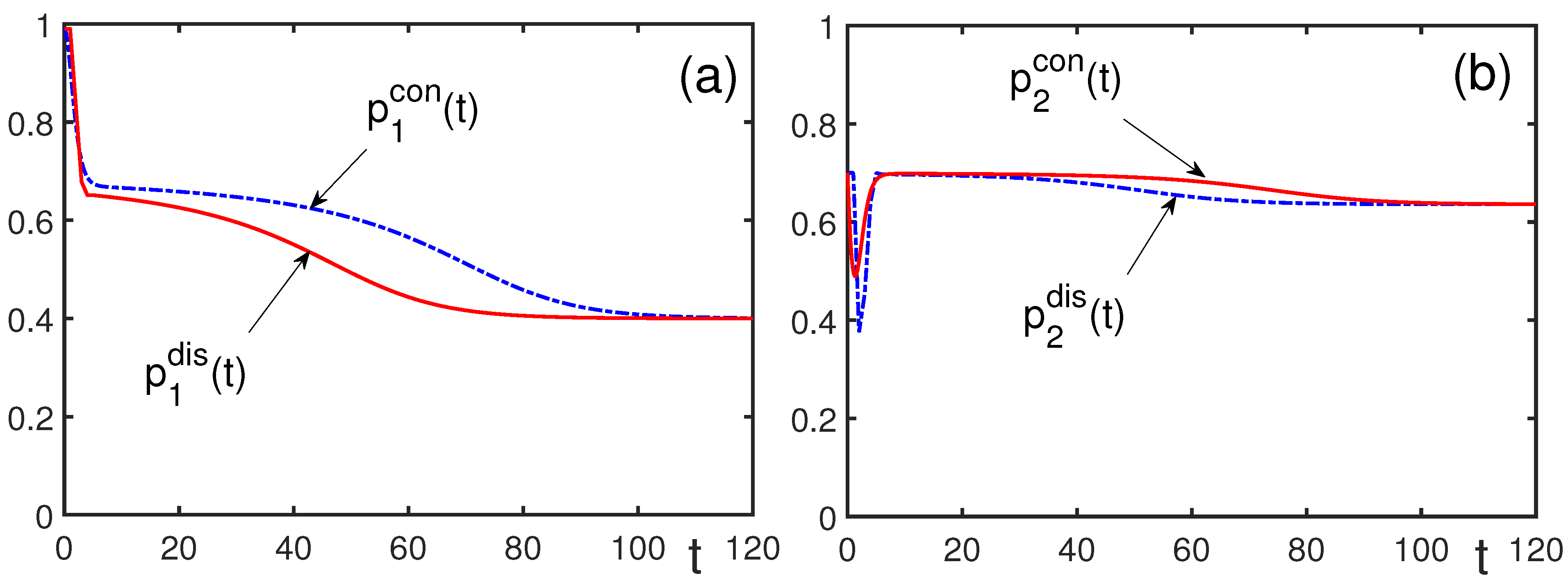
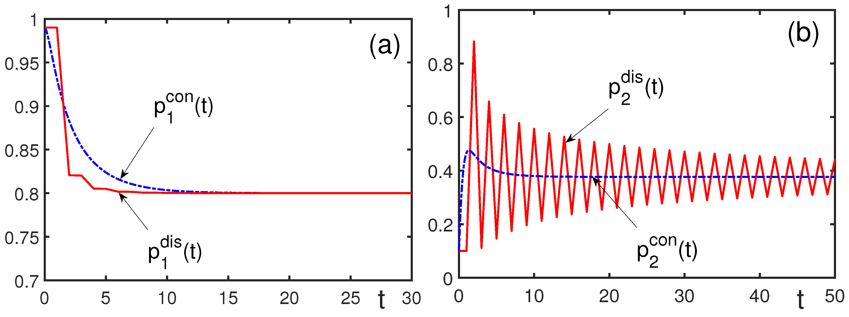
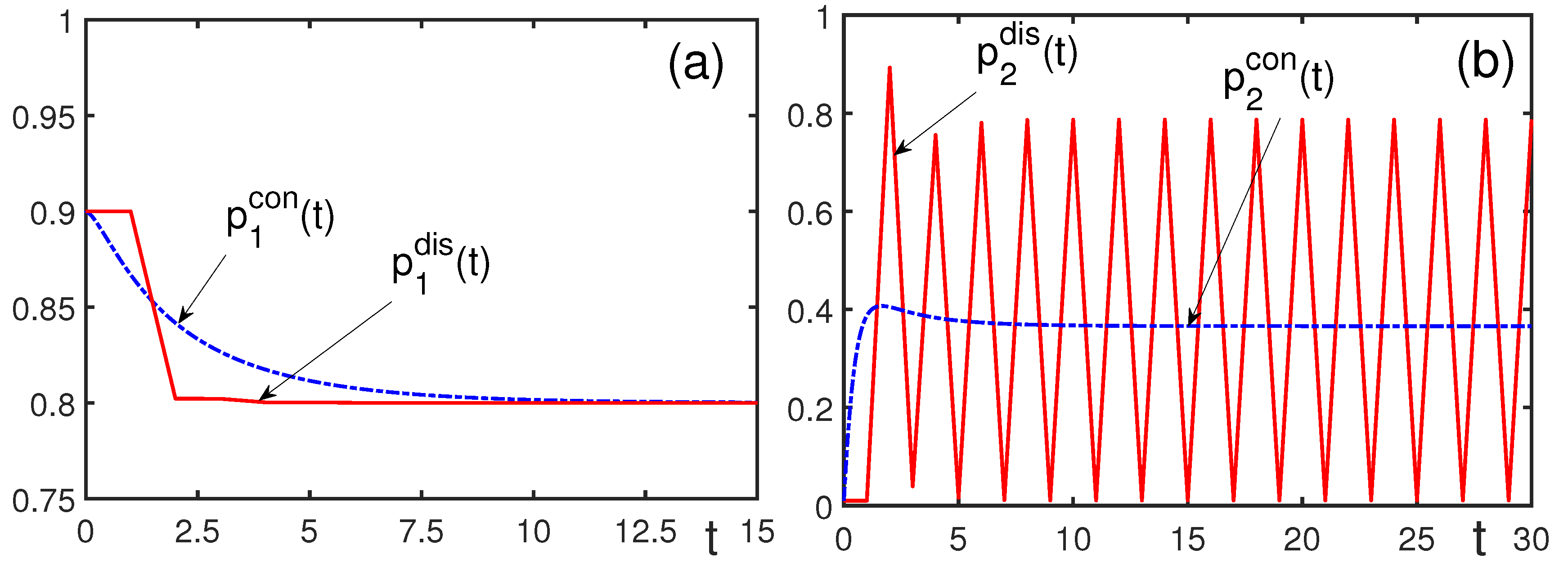
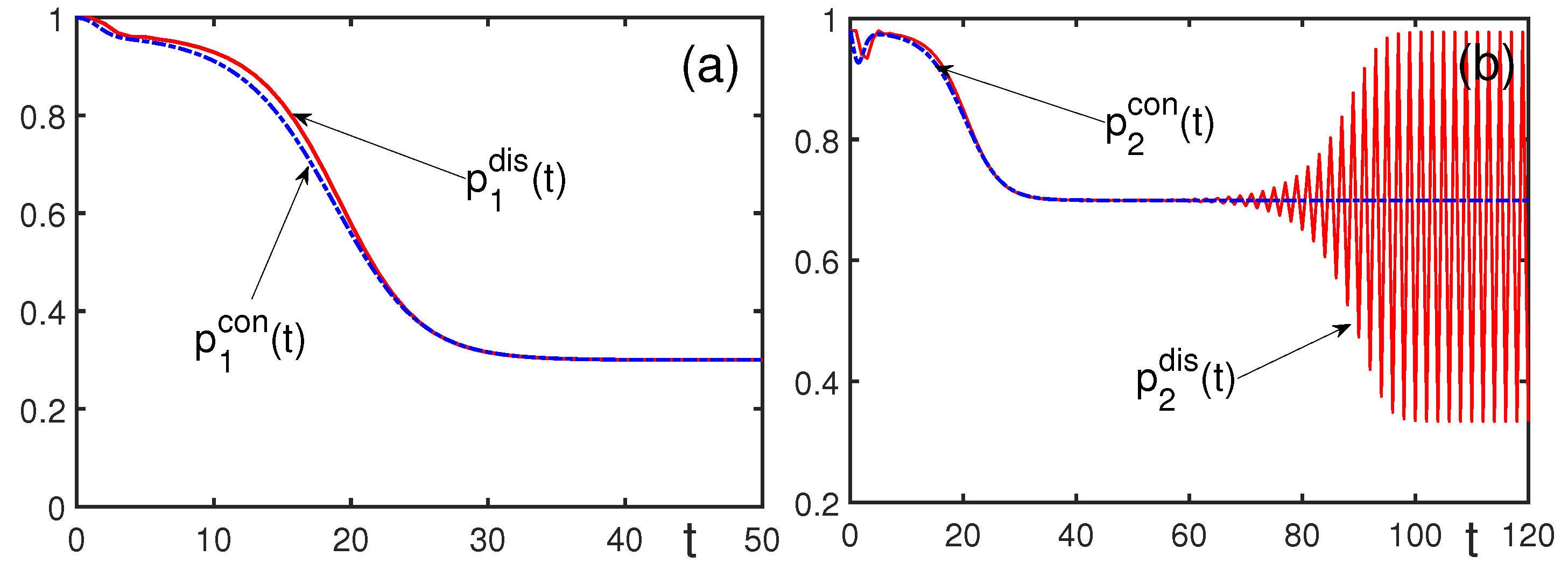
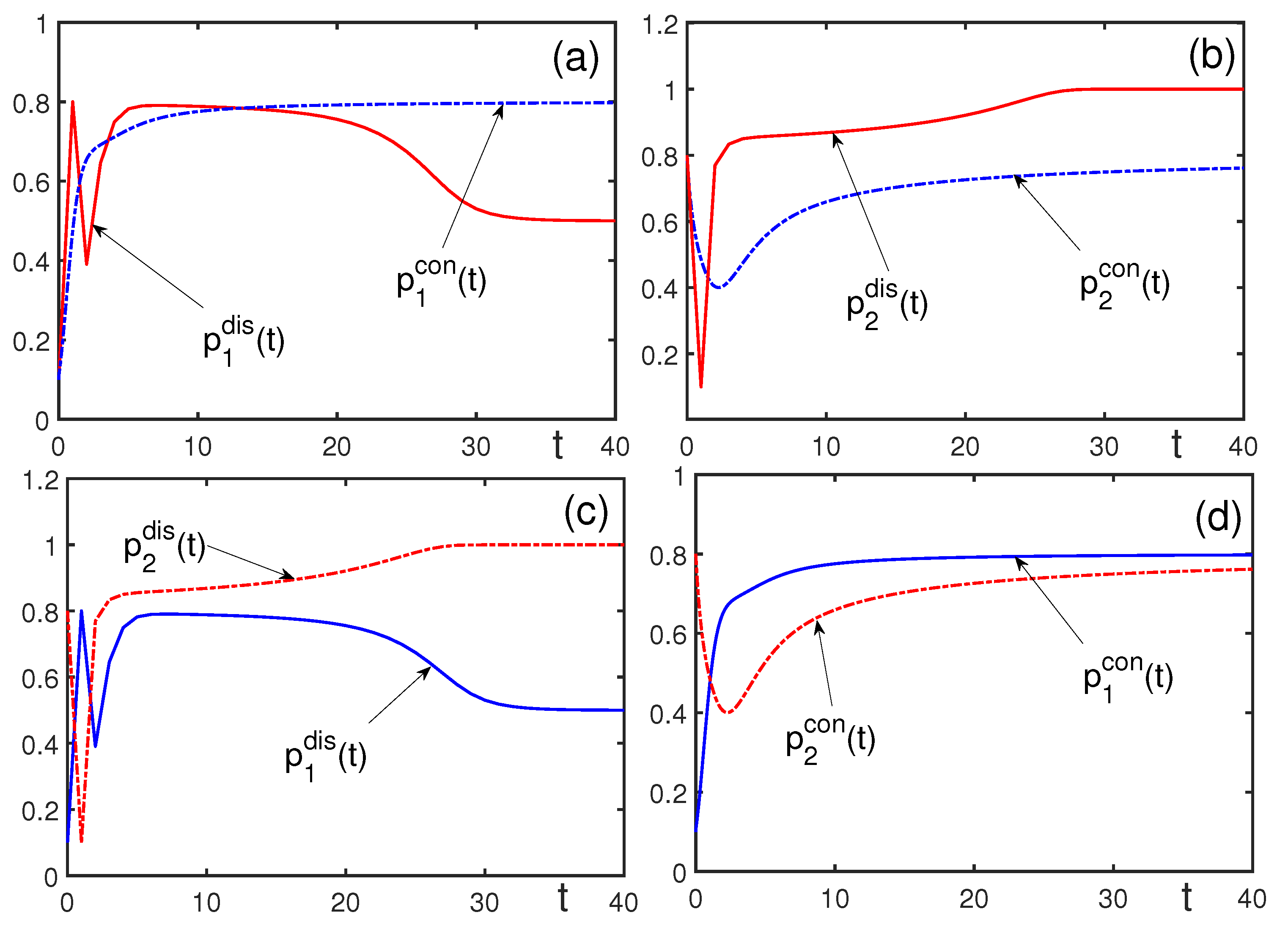
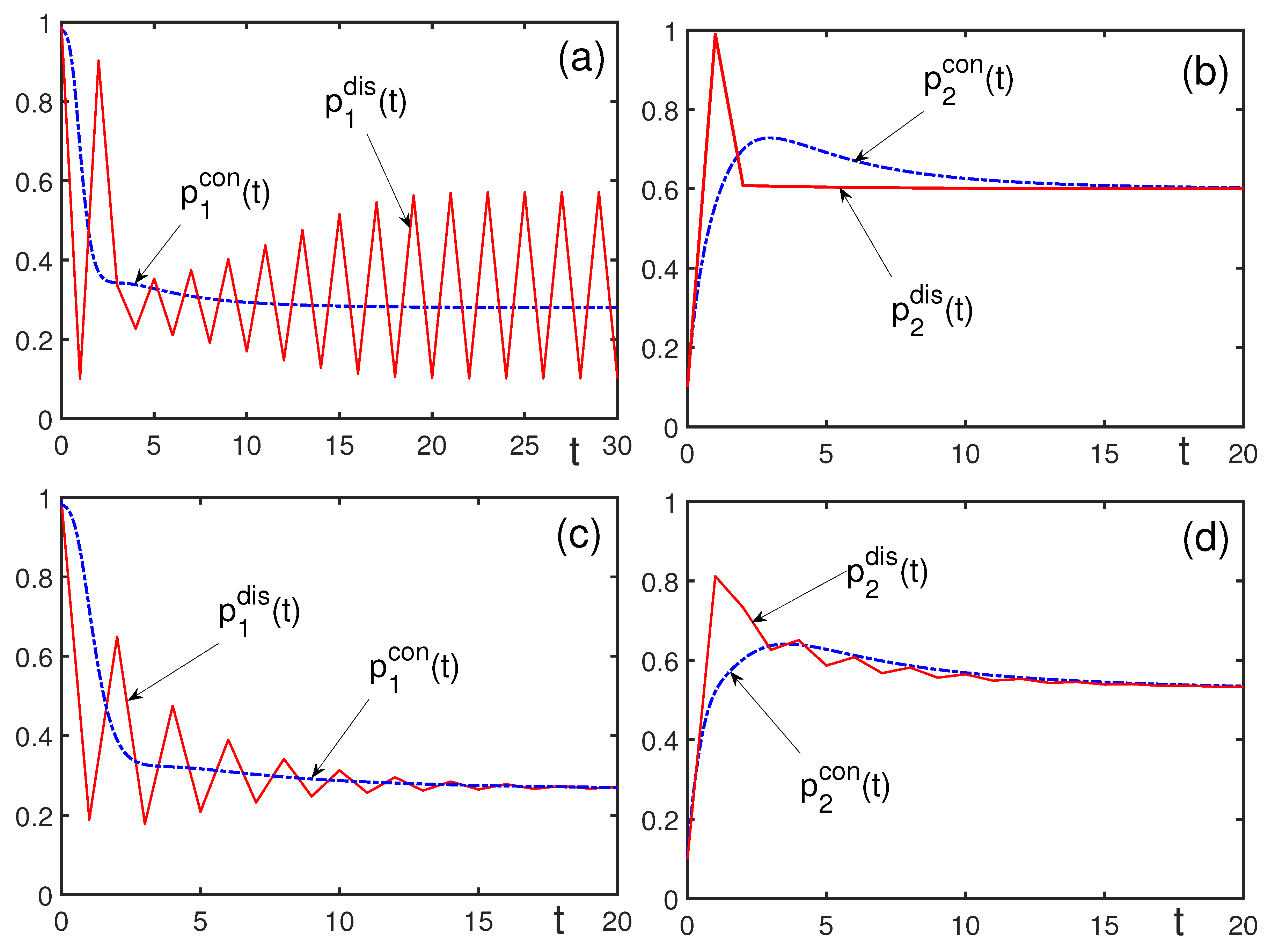
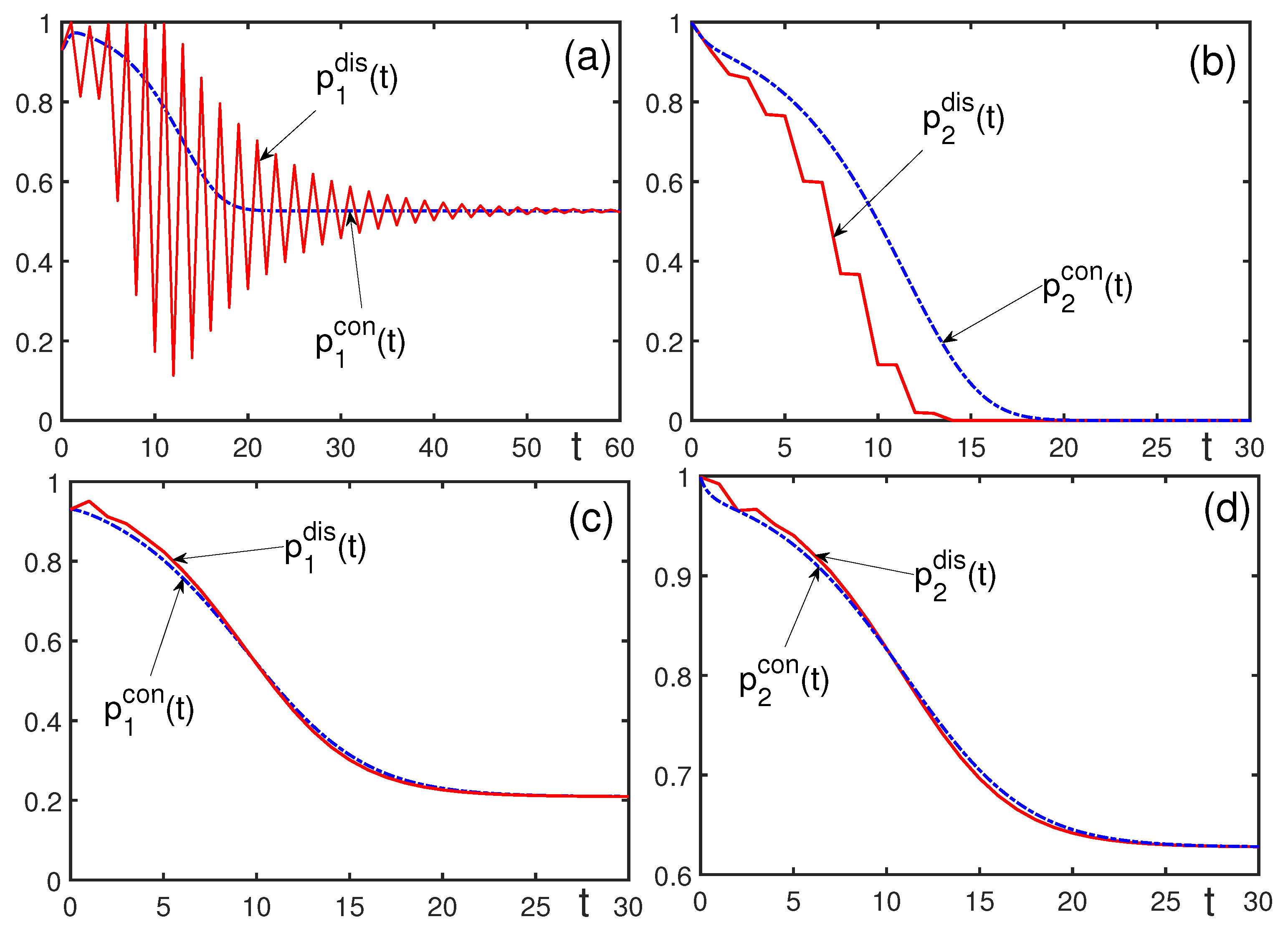
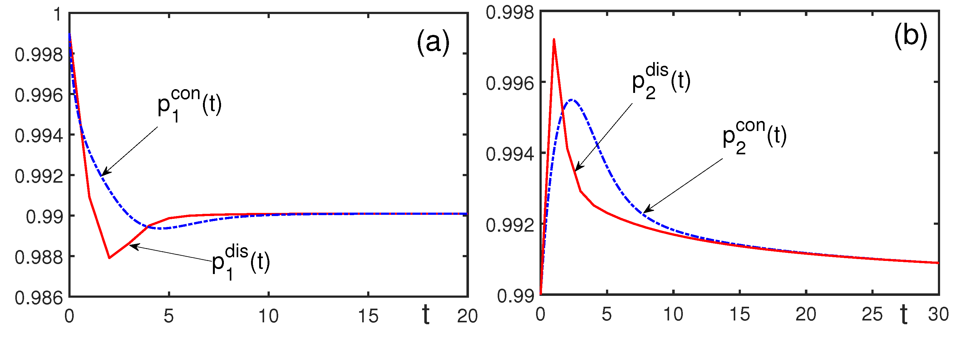
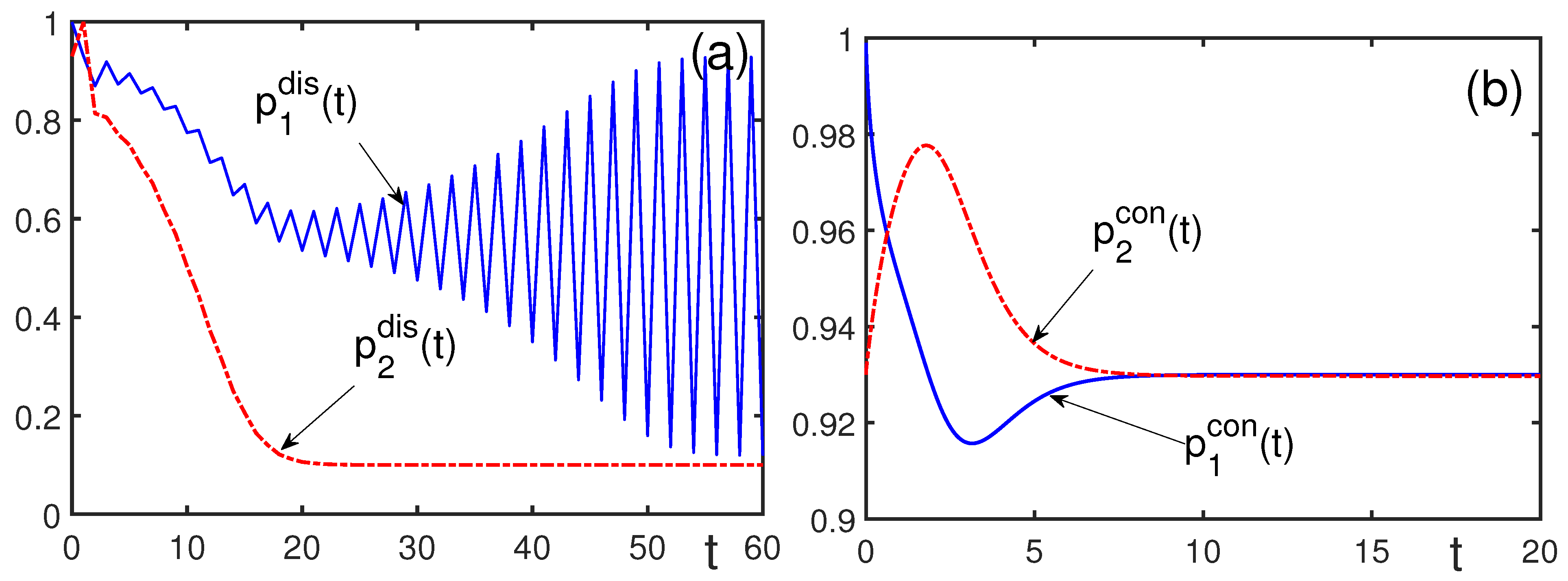
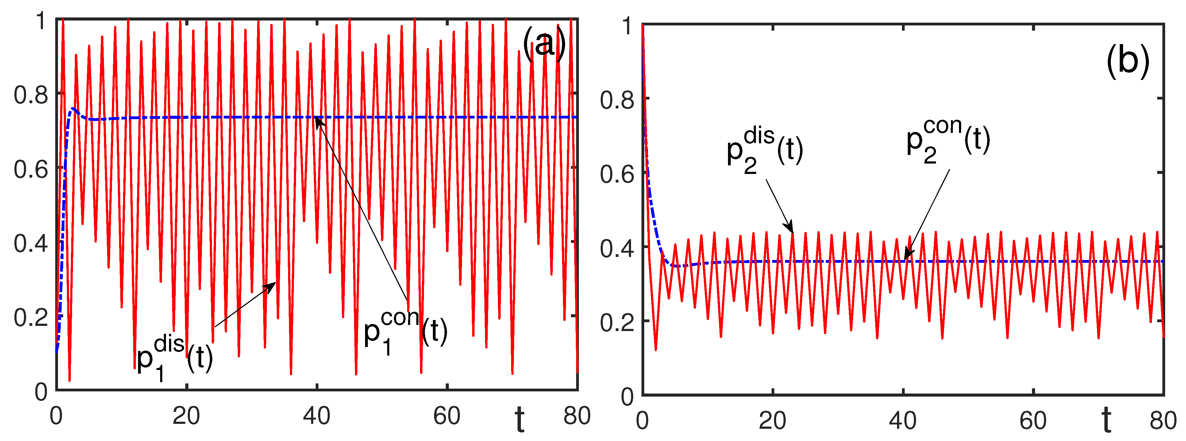
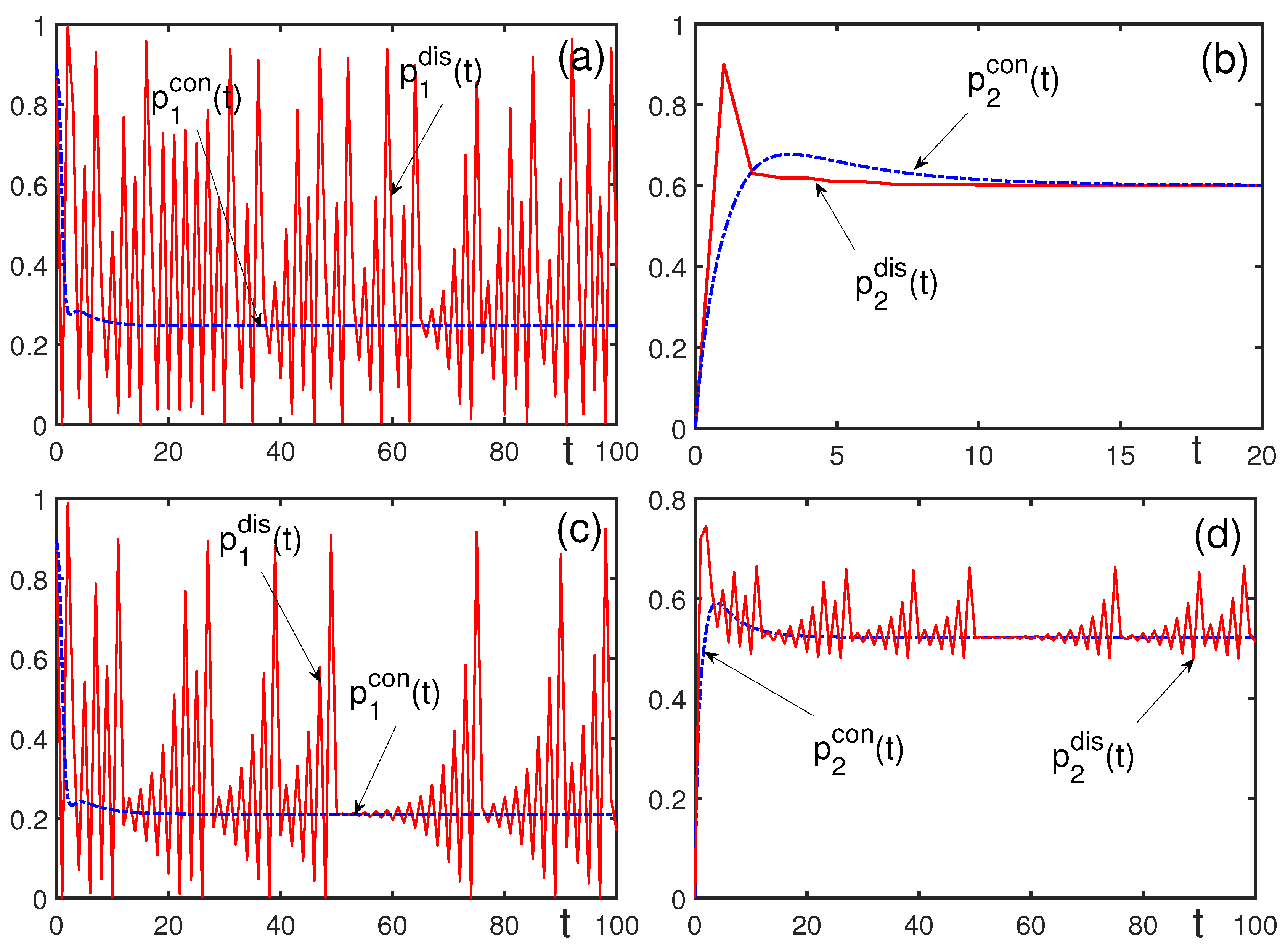
6. Comparison of Discrete versus Continuous Algorithms

Formally, it looks that the fixed points, if they exist, of the discrete (37) and continuous (43) dynamical systems are the same, being given by the equations

$$p_1^{\ast }=(1-{\epsilon }_1)(f_1+q_1^{\ast })+{\epsilon }_1(f_2+q_2^{\ast }),$$

$$p_2^{\ast }=(1-{\epsilon }_2)(f_2+q_2^{\ast })+{\epsilon }_2(f_1+q_1^{\ast }),$$

(46)

where $q_j^{\ast }$ is the limit of $q_j\left(t\right)$ as time goes to infinity. However, strictly speaking, the discrete and continuous limits can be different, since the related expressions for the memory functions in the discrete and continuous cases are different. Also, the considered equations are not autonomous and contain time delay. In addition, even if the fixed points would be the same, the stability conditions of discrete, continuous, and delay equations, generally, are different [73,74,75]. Thus, numerical investigations are necessary.

We have compared the solutions to discrete-time Equation (37) and continuous-time Equation (43), for the same sets of parameters and initial conditions. The society is composed of two groups, one whose members enjoy long-term memory and the other group, consists of members with short-term memory. Solutions for discrete equations are marked as $p_j^{dis}\left(t\right)$ and for continuous equations as $p_j^{con}\left(t\right)$. In all figures, time is dimensionless, being measured in units of $\tau$. The results are discussed below.

Figure 1 presents the case where the fractions (probabilities) $p_j^{con}\left(t\right)$ and $p_j^{dis}\left(t\right)$ starting from the same values smoothly tend to the same fixed points, being only slightly different at intermediate times.

Figure 2 shows the situation when the probabilities of choosing an alternative by agents with long-term memory smoothly tend to the same fixed point, but the probabilities for agents with short-term memory, although tending to the same fixed point, tend in a rather different way. The continuous solution tends smoothly, while the discrete solution, through oscillations.

Figure 3 demonstrates that the fixed points of discrete and continuous solutions can be of different nature. Thus, for the group of agents with long-term memory, the discrete and continuous solutions tend to the same stable node. However, for the agents with short-term memory, it is a stable node for the continuous solution, but a center for the discrete solution.

Figure 4 shows that the fixed points of agents with long-term memory can coincide for discrete and continuous solutions, both being stable nodes, while for agents with short-term memory, the continuous solution tends to a stable node, whereas the discrete solution at the beginning almost coincides with the continuous one, but starts oscillating from a finite time and after this continues oscillating for all times.

Figure 5 explains that discrete and continuous probabilities, though both being stable nodes, tend to different fixed points, which do not coincide. This happens in the presence of a strong herding effect.

Figure 6 and Figure 7 illustrate qualitatively different behaviors of discrete and continuous solutions in the presence of the herding effect, when the related $p_j^{dis}\left(t\right)$ and $p_j^{con}\left(t\right)$ can either tend to coinciding stable nodes or $p_j^{dis}\left(t\right)$ can exhibit oscillations, while $p_j^{con}\left(t\right)$ smoothly tends to a stable node.

Figure 8 shows a rare case, where all probabilities for the groups with long-term memory as well as short-term memory, for discrete as well as continuous solutions, tend to the common fixed point $p_{1dis}^{\ast }=p_{1con}^{\ast }=p_{2dis}^{\ast }=p_{2con}^{\ast }=f_2+q_2=0.99$.

Figure 9 gives an example where continuous solutions for both groups, with long-term and short-term memory, can tend to coinciding limits, while the related discrete solutions for these groups are very different: One solution permanently oscillates, and the other tends to a stable node.

Finally, Figure 10 and Figure 11 demonstrate the possibility of chaotic behavior for discrete solutions, when, for the same parameters, continuous solutions smoothly converge to stable nodes.

Summarizing the possible types of behavior, we see that continuous decision making always displays smooth behavior of probabilities for both groups, with either long-term or short-term memory always converging to a stable node. However, discrete decision making can exhibit, for the same probabilities, a larger variety of behavior types, which can be smooth, tending to a stable node, or oscillating, hence tending to a stable focus, or even chaotic.

As far as the temporal behavior of the probabilities of choosing the related alternatives for discrete and continuous decision making can be essentially different, the natural question arises: Which of the algorithms, discrete or continuous, better corresponds to the real decision making of social groups? It seems there are activities, such as car driving, where decisions can be well approximated by a continuous process. At the same time, it looks like such processes can be described by a series of decisions occurring discretely, although with rather small time intervals between the subsequent steps. It may happen that, despite the small time intervals, the discrete and continuous decision algorithms lead to different conclusions. From our point of view, the discrete algorithm is preferable, since decisions, anyway, are complex, discrete actions composed of several subactions: receiving information, processing this information, and making a decision, so that always there is a delay time from the start of receiving information to the moment of making a decision. The continuous algorithm can provide a reasonable approximation in some cases, although sometimes can result in wrong conclusions.

When a probability $p_j\left(t\right)$ converges to a stable node, the corresponding stationary limit $p_j^{\ast }$ plays the role of the optimal decision taken after multiple steps of decision making, including the exchange of information with other agents of all groups, taking account of agents’ emotions, and the tendency of the agents to herding. When a probability oscillates either periodically or chaotically, this implies that the agents are not able to come to a decision, but cannot stop hesitating. There exist numerous examples of chaotic behavior of decision making in medicine, economics, and different types of management [76,77,78,79,80,81,82,83,84,85,86,87].

The mathematical reason why the considered continuous solutions for the probabilities cannot display chaos is as follows. The probabilities, by definition, are bounded, hence Lagrange stable. Then, for a plane motion, the Poincare–Bendixson theorem tells us that if a trajectory of a continuous two-dimensional dynamical system is Lagrange stable, then it approaches either a stable node or a limit cycle [75]. However, for discrete equations, there is no such theorem, and a discrete dynamical system can exhibit chaos.

7. Conclusions

We have considered affective dynamic decision making, where there are several groups of agents choosing between several alternatives. A multistep process of decision making takes into account the utility of the alternatives, their attractiveness, and the inclination of the society members to mimic the actions of others (herding effect). Two possible algorithms are compared, one algorithm treating multistep decision making as a sequence of discrete decisions, while the other algorithm studies the overall process as one continuous action. Dynamic regimes of both algorithms are thoroughly investigated for the case of two alternatives and two groups of agents. One group consists of agents with long-term memory and the other, of agents with short-term memory.

It is worth stressing that our aim has been not a study of some specific cases, but the general understanding of which of the possible algorithms is more appropriate for the description in a wide range of parameters corresponding to different situations.

It turns out that the discrete algorithm exhibits much richer behavior that includes the tendency to a stable node, or to stable focus, or to chaotic behavior. Contrary to this, the continuous algorithm always results in the convergence to a stable node. In real life, as empirical studies show, chaotic decision making can occur in the presence of risk and uncertainty. Therefore, it appears that the discrete algorithm is more general, while the continuous algorithm can be treated as an approximation that in some cases gives a reasonable description, while in many other cases it is not applicable. Anyway, from the physiological point of view, multistep decision making better corresponds to a sequence of separate decisions than to a single continuous action.

For clarity, above, we kept in mind the frequentist interpretation of probability as a fraction of group members. As far as the decision making of a single agent is also a probabilistic process, the theory can also be applied to separate agents possessing different types of memory.

Instead of separate agents, it is possible to consider the nodes of an intelligent network. For instance, one can keep in mind a neural network, where neurons exchange information in order to come to a state represented by a fixed point. The chaotic performance of an intelligent network can be interpreted as due to some uncertainty in the process of choice. For humans, uncertainty can be caused by the complexity of the studied problem or by defects in a neural network. Overall, affective intelligence, whether artificial or natural, seems to be better described by discrete algorithms than by their continuous approximations. The results of this paper can be useful for the creation of affective artificial intelligence.

The probabilistic model of affective decision making, considered in this paper, can be extended in several aspects. It is possible to include into consideration more than two groups, for instance differing from each other by memory longevity or by the strength of mutual interactions in the process of exchanging information. It is also possible to take into account time discounting diminishing the utility factors with time. These extensions are planned for future research.

References

1. Turkle, S. The Second Self: Computers and the Human Spirit; Granada: London, UK, 1984. [Google Scholar]
2. Brehmer, B. Dynamic decision making: Human control of complex systems. Psychologica 1992, 81, 211–241. [Google Scholar] [CrossRef] [PubMed]
3. Beresford, B.; Sloper, T. Understanding the Dynamics of Decision-Making and Choice: A Scoping Study of Key Psychological Theories to Inform the Design and Analysis of the Panel Study; University of York: York/Heslington, UK, 2008. [Google Scholar]
4. Evertsz, R.; Thangarajah, J.; Ly, T. Practical Modelling of Dynamic Decision Making; Springer: Cham, Switzerland, 2019. [Google Scholar]
5. Perc, M.; Gomez-Gardenes, J.; Szolnoki, A.; Floria, L.M.; Moreno, Y. Evolutionary dynamics of group interactions on structured populations: A review. J. R. Soc. Interface 2013, 10, 20120997. [Google Scholar] [CrossRef] [PubMed]
6. Perc, M.; Jordan, J.J.; Rand, D.G.; Wang, Z.; Boccaletti, S.; Szolnoki, A. Statistical physics of human cooperation. Phys. Rep. 2017, 687, 1–51. [Google Scholar] [CrossRef]
7. Capraro, V.; Perc, M. Mathematical foundations of moral preferences. J. R. Soc. Interface 2021, 18, 20200880. [Google Scholar] [CrossRef] [PubMed]
8. Jusup, M.; Holme, P.; Kanazawa, K.; Takayasu, M.; Romic, I.; Wang, Z.; Gecek, S.; Lipic, T.; Podobnik, B.; Wang, L.; et al. Social physics. Phys. Rep. 2022, 948, 1–148. [Google Scholar] [CrossRef]
9. Yukalov, V.I. A resolution of St. Petersburg paradox. J. Math. Econ. 2021, 97, 102537. [Google Scholar] [CrossRef]
10. Yukalov, V.I. Quantification of emotions in decision making. Soft Comput. 2022, 26, 2419–2436. [Google Scholar] [CrossRef]
11. Yukalov, V.I. Quantum operation of affective artificial intelligence. Laser Phys. 2023, 33, 065204. [Google Scholar] [CrossRef]
12. Gonzalez, C.; Vanyukov, P.; Martin, M.K. The use of microworlds to study dynamic decision making. Comput. Hum. Behav. 2005, 21, 273–286. [Google Scholar] [CrossRef]
13. Barendregt, N.W.; Josić, K.; Kilpatrick, Z.P. Analyzing dynamic decision-making models using Chapman-Kolmogorov equations. J. Comput. Neurosci. 2019, 47, 205–222. [Google Scholar] [CrossRef]
14. Behrens, T.E.; Woolrich, M.W.; Walton, M.E.; Rushworth, M.F. Learning the value of information in an uncertain world. Nat. Neurosci. 2007, 10, 1214. [Google Scholar] [CrossRef] [PubMed]
15. Ossmy, O.; Moran, R.; Pfeffer, T.; Tsetsos, K.; Usher, M.; Donner, T.H. The timescale of perceptual evidence integration can be adapted to the environment. Curr. Biol. 2013, 23, 981–986. [Google Scholar] [CrossRef]
16. Yu, A.J.; Cohen, J.D. Sequential effects: Superstition or rational behavior? Adv. Neural Inform. Process. Syst. 2008, 21, 1873–1880. [Google Scholar]
17. Brea, J.; Urbanczik, R.; Senn, W. A normative theory of forgetting: Lessons from the fruit fly. PLoS Comput. Biol. 2014, 10, 1003640. [Google Scholar] [CrossRef] [PubMed]
18. Urai, A.E.; Braun, A.; Donner, T.H. Pupil-linked arousal is driven by decision uncertainty and alters serial choice bias. Nature Commun. 2017, 8, 14637. [Google Scholar] [CrossRef]
19. Baddeley, A. Working Memory, Thought, and Action; Oxford University Press: Oxford, UK, 2007. [Google Scholar]
20. Albrecht, S.V.; Christianos, F.; Schäfer, L. Multi-Agent Reinforcement Learning: Foundations and Modern Approaches; Massachusetts Institute of Technology: Cambridge, MA, USA, 2023. [Google Scholar]
21. Von Neumann, J.; Morgenstern, O. Theory of Games and Economic Behavior; Princeton University Press: Princeton, NJ, USA, 1953. [Google Scholar]
22. Savage, L.J. The Foundations of Statistics; Wiley: New York, NY, USA, 1954. [Google Scholar]
23. Kurtz-David, V.; Persitz, D.; Webb, R.; Levy, D.J. The neural computation of inconsistent choice behaviour. Nat. Commun. 2019, 10, 1583. [Google Scholar] [CrossRef]
24. Yaari, M.E. The dual theory of choice under risk. Econometrica 1987, 55, 95–115. [Google Scholar] [CrossRef]
25. Reynaa, V.F.; Brainer, C.J. Dual processes in decision making and developmental neuroscience: A fuzzy-trace model. Developm. Rev. 2011, 31, 180–206. [Google Scholar] [CrossRef] [PubMed]
26. Woodford, M. Modeling imprecision in perception, valuation and choice. Annu. Rev. Econ. 2020, 12, 579–601. [Google Scholar] [CrossRef]
27. Luce, R.D. Individual Choice Behavior: A Theoretical Analysis; Wiley: New York, NY, USA, 1959. [Google Scholar]
28. Luce, R.D.; Raiffa, R. Games and Decisions: Introduction and Critical Survey; Dover: New York, NY, USA, 1989. [Google Scholar]
29. Brandt, R.B. The concept of rational belief. Monist 1985, 68, 3–23. [Google Scholar] [CrossRef]
30. Swinburne, R. Faith and Reason; Oxford University: Oxford, UK, 2005. [Google Scholar]
31. Steuer, R.E. Multiple Criteria Optimization: Theory, Computation and Application; Wiley: New York, NY, USA, 1986. [Google Scholar]
32. Triantaphyllou, E. Multi-Criteria Decision Making: A Comparative Study; Kluwer: Dordrecht, The Netherlands, 2000. [Google Scholar]
33. Köksalan, M.; Wallenius, J.; Zionts, S. Multiple Criteria Decision Making: From Early History to the 21st Century; World Scientific: Sinapore, 2011. [Google Scholar]
34. Basilio, M.P.; Pereira, V.; Costa, H.G.; Santos, M.; Ghosh, A. A systematic review of the applications of multi-criteria decision aid methods (1977–2022). Electronics 2022, 11, 1720. [Google Scholar] [CrossRef]
35. Yukalov, V.I.; Yukalova, E.P.; Sornette, D. Information processing by networks of quantum decision makers. Phys. A 2018, 492, 747–766. [Google Scholar] [CrossRef]
36. Yukalov, V.I.; Yukalova, E.P.; Sornette, D. Role of collective information in networks of quantum operating agents. Phys. A 2022, 598, 127365. [Google Scholar] [CrossRef]
37. Yukalov, V.I.; Yukalova, E.P. Self-excited waves in complex social systems. Physica D 2022, 433, 133188. [Google Scholar] [CrossRef]
38. Martin, E.D. The Behavior of Crowds: A Psychological Study; Harper & Brothers: New York, NY, USA, 1920. [Google Scholar]
39. Sherif, M. The Psychology of Social Norms; Harper & Brothers: New York, NY, USA, 1936. [Google Scholar]
40. Smelser, N.J. Theory of Collective Behavior; Macmillan: New York, NY, USA, 1965. [Google Scholar]
41. Merton, R.K. Social Theory and Social Structure; Macmillan: New York, NY, USA, 1968. [Google Scholar]
42. Turner, R.H.; Killian, L.M. Collective Behavior; Prentice-Hall: Englewood Cliffs, NJ, USA, 1993. [Google Scholar]
43. Hatfield, E.; Cacioppo, J.T.; Rapson, R.L. Emotional Contagion; Cambridge University Press: New York, NY, USA, 1993. [Google Scholar]
44. Brunnermeier, M.K. Asset Pricing under Asymmetric Information: Bubbles, Crashes, Technical Analysis, and Herding; Oxford University Press: New York, NY, USA, 2001. [Google Scholar]
45. Sornette, D. Why Stock Markets Crash; Princeton University Press: Princeton, NJ, USA, 2003. [Google Scholar]
46. Yukalov, V.I. Selected topics of social physics: Equilibrium systems. Physics 2023, 5, 590–635. [Google Scholar] [CrossRef]
47. Yukalov, V.I.; Sornette, D. Manupulating decision making of typical agents. IEEE Trans. Syst. Man Cybern. Syst. 2014, 44, 1155–1168. [Google Scholar] [CrossRef]
48. Yukalov, V.I.; Sornette, D. Quantitative predictions in quantum decision theory. IEEE Trans. Syst. Man Cybern. Syst. 2018, 48, 366–381. [Google Scholar] [CrossRef]
49. Read, D.; Loewenstein, G. Time and decision: Introduction to the special issue. J. Behav. Decis. Mak. 2000, 13, 141–144. [Google Scholar] [CrossRef]
50. Frederick, S.; Loewenstein, G.; O’Donoghue, T. Time discounting and time preference: A critical review. J. Econ. Liter. 2002, 40, 351–401. [Google Scholar] [CrossRef]
51. Yukalov, V.I.; Sornette, D. Role of information in decision making of social agents. Int. J. Inform. Technol. Decis. Mak. 2015, 14, 1129–1166. [Google Scholar] [CrossRef]
52. Kühberger, A.; Komunska, D.; Perner, J. The disjunction effect: Does it exist for two-step gambles? Org. Behav. Human Decis. Process. 2001, 85, 250–264. [Google Scholar] [CrossRef]
53. Charness, G.; Rabin, M. Understanding social preferences with simple tests. Quart. J. Econ. 2002, 117, 817–869. [Google Scholar] [CrossRef]
54. Cooper, D.; Kagel, J. Are two heads better than one? Team versus individual play in signaling games. Am. Econ. Rev. 2005, 95, 477–509. [Google Scholar] [CrossRef]
55. Blinder, A.; Morgan, J. Are two heads better than one? An experimental analysis of group versus individual decision-making. J. Money Credit Bank. 2005, 37, 789–811. [Google Scholar]
56. Sutter, M. Are four heads better than two? An experimental beauty-contest game with teams of different size. Econ. Lett. 2005, 88, 41–46. [Google Scholar] [CrossRef]
57. Tsiporkova, E.; Boeva, V. Multi-step ranking of alternatives in a multi-criteria and multi-expert decision making environment. Inform. Sci. 2006, 176, 2673–2697. [Google Scholar] [CrossRef]
58. Charness, G.; Karni, E.; Levin, D. Individual and group decision making under risk: An experimental study of Bayesian updating and violations of first-order stochastic dominance. J. Risk Uncert. 2007, 35, 129–148. [Google Scholar] [CrossRef]
59. Charness, G.; Rigotti, L.; Rustichini, A. Individual behavior and group membership. Am. Econ. Rev. 2007, 97, 1340–1352. [Google Scholar] [CrossRef]
60. Chen, Y.; Li, S. Group identity and social preferences. Am. Econ. Rev. 2009, 99, 431–457. [Google Scholar] [CrossRef]
61. Liu, H.H.; Colman, A.M. Ambiguity aversion in the long run: Repeated decisions under risk and uncertainty. J. Econ. Psychol. 2009, 30, 277–284. [Google Scholar] [CrossRef]
62. Charness, G.; Karni, E.; Levin, D. On the conjunction fallacy in probability judgement: New experimental evidence regarding Linda. Games Econ. Behav. 2010, 68, 551–556. [Google Scholar] [CrossRef]
63. Sung, S.Y.; Choi, J.N. Effects of team management on creativity and financial performance of organizational teams. Org. Behav. Human Decis. Process. 2012, 118, 4–13. [Google Scholar] [CrossRef]
64. Schultze, T.; Mojzisch, A.; Schulz-Hardt, S. Why groups perform better than individuals at quantitative judgement tasks. Org. Behav. Human Decis. Process. 2012, 118, 24–36. [Google Scholar] [CrossRef]
65. Xu, Z. Approaches to multi-stage multi-attribute group decision making. Int. J. Inf. Technol. Decis. Mak. 2011, 10, 121–146. [Google Scholar] [CrossRef]
66. Tapia Garcia, J.M.; Del Moral, M.J.; Martinez, M.A.; Herrera-Viedma, E. A consensus model for group decision-making problems with interval fuzzy preference relations. Int. J. Inf. Technol. Decis. Mak. 2012, 11, 709–725. [Google Scholar] [CrossRef]
67. Kullback, S.; Leibler, R.A. On information and sufficiency. Ann. Math. Stat. 1951, 22, 79–86. [Google Scholar] [CrossRef]
68. Kullback, S. Information Theory and Statistics; Peter Smith: Gloucester, MA, USA, 1978. [Google Scholar]
69. James, W. The Principles of Psychology; Holt: New York, NY, USA, 1890. [Google Scholar]
70. Fitts, P.M.; Posner, M.I. Human Performance; Brooks/Cole: Boston, MA, USA, 1967. [Google Scholar]
71. Cowan, N. What are the differences between long-term, short-term, and working memory. Prog. Brain Res. 2008, 169, 323–338. [Google Scholar]
72. Camina, E.; Güell, F. The neuroanatomical, neurophysiological and psychological basis of memory: Current models and their origins. Front. Pharmacol. 2017, 8, 438. [Google Scholar] [CrossRef]
73. Gershenfeld, N.A. The Nature of Mathematical Modeling; Cambridge University Press: Cambridge, UK, 1999. [Google Scholar]
74. Matsumoto, A.; Szidarovszky, F. Dynamic Oligopolicies with Time Delays; Springer: Singapore, 2018. [Google Scholar]
75. Yukalov, V.I. Selected topics of social physics: Nonequilibrium systems. Physics 2023, 5, 704–751. [Google Scholar] [CrossRef]
76. Baumol, W.; Benhabib, J. Chaos: Significance, mechanism, and economic applications. J. Econ. Perspect. 1989, 3, 77–105. [Google Scholar] [CrossRef]
77. Mayer-Kress, G.; Grossman, S. Chaos in the international arms race. Nature 1989, 337, 701–704. [Google Scholar]
78. Richards, D. Is strategic decision making chaotic? Behav. Sci. 1990, 35, 219–232. [Google Scholar] [CrossRef]
79. Radzicki, M.J. Institutional dynamics, deterministic chaos, and self-organizing systems. J. Econ. Issues 1990, 24, 57–102. [Google Scholar] [CrossRef]
80. Goldberger, A.L.; Rigney, D.R.; West, B.J. Chaos and fractals in physiology. Sci. Am. 1990, 263, 43–49. [Google Scholar]
81. Cartwright, T.J. Planning and chaos theory. J. Am. Plann. Assoc. 1991, 57, 44–56. [Google Scholar] [CrossRef]
82. Levy, D. Chaos theory and strategy: Theory, application, and managerial implications. Strateg. Manag. J. 1994, 15, 167–178. [Google Scholar] [CrossRef]
83. Barton, S. Chaos, self-organization, and psychology. Am. Psychol. 1994, 49, 5–14. [Google Scholar] [CrossRef]
84. Krippner, S. Humanistic psychology and chaos theory: The third revolution and the third force. J. Human. Psychol. 1994, 34, 48–61. [Google Scholar] [CrossRef]
85. Marion, R. The Edge of Organisations: Chaos and Complexity Theories of Formal Social Systems; Sage Publications: Thousand Oaks, CA, USA, 1999. [Google Scholar]
86. McKenna, R.J.; Martin-Smith, B. Decision making as a simplification process: New conceptual perspectives. Manag. Decis. 2005, 43, 821–836. [Google Scholar] [CrossRef]
87. McBride, N. Chaos theory as a model for interpreting information systems in organisations. Inform. Syst. J. 2005, 15, 233–254. [Google Scholar] [CrossRef]
Figure 1. Solutions to discrete Equation (37) and to continuous Equation (43) for the initial conditions f 1 = 0.4 , f 2 = 0.1 , q 1 = 0.59 , and q 2 = 0.6 , in the absence of herding effect, when ε 1 = ε 2 = 0 : (a) Discrete solution p 1 d i s ( t ) (solid line) and continuous solution p 1 c o n ( t ) (dashed-dotted line). Both solutions tend to the same fixed point p 1 = 0.4 ; (b) Discrete solution p 2 d i s ( t ) (solid line) and continuous solution p 2 c o n ( t ) (dashed-dotted line). Both solutions tend to the same fixed point p 2 = 0.636 , which is a stable node.
Algorithms 16 00416 g001
Figure 2. Solutions to discrete Equation (37) and to continuous Equation (43) for the initial conditions f 1 = 0.8 , f 2 = 0.9 , q 1 = 0.19 , and q 2 = 0.8 , when there is no herding effect, hence ε 1 = ε 2 = 0 : (a) Discrete solution p 1 d i s ( t ) (solid line) and continuous solution p 1 c o n ( t ) (dashed-dotted line). Both solutions tend to the same fixed point p 1 = 0.8 ; (b) Discrete solution p 2 d i s ( t ) (solid line) and continuous solution p 2 c o n ( t ) (dashed-dotted line). Probability p 2 c o n ( t ) tends monotonically, while p 2 d i s ( t ) tends with oscillations to the same fixed point p 2 = 0.377 . Discrete and continuous solutions tend to the same fixed point, but for the agents with long-term memory the fixed point is a stable node, however for the agents with short-term memory, the continuous solution tends to a stable node, while for the discrete solution, to a stable focus.
Algorithms 16 00416 g002
Figure 3. Solutions to discrete Equation (37) and to continuous Equation (43) for the initial conditions f 1 = 0.8 , f 2 = 1 , q 1 = 0.1 , and q 2 = 0.99 , in the absence of herding effect, when ε 1 = ε 2 = 0 : (a) Discrete solution p 1 d i s ( t ) (solid line) and continuous solution p 1 c o n ( t ) (dashed-dotted line). Solutions p 1 c o n ( t ) and p 1 d i s ( t ) tend to the same fixed point p 1 = 0.8 ; (b) Discrete solution p 2 d i s ( t ) (solid line) and continuous solution p 2 c o n ( t ) (dashed-dotted line). Solution p 2 c o n ( t ) tends to the fixed point p 2 = 0.366 , whereas p 2 d i s ( t ) oscillates around p 2 with the constant amplitude. For the agents with long-term memory, both probabilities, discrete and continuous, tend to the same stable node, but for the agents with short-term memory, the fixed point for discrete probability is a stable limit cycle, while the continuous probability tends to a stable node.
Algorithms 16 00416 g003
Figure 4. Solutions to discrete Equation (37) and to continuous Equation (43) for the initial conditions f 1 = 0.3 , f 2 = 0 , q 1 = 0.699 , and q 2 = 0.98 , without the herding effect, when ε 1 = ε 2 = 0 : (a) Discrete solution p 1 d i s ( t ) (solid line) and continuous solution p 1 c o n ( t ) (dashed-dotted line). Solutions p 1 c o n ( t ) and p 1 d i s ( t ) tend to the same fixed point p 1 = 0.3 ; (b) Discrete solution p 2 d i s ( t ) (solid line) and continuous solution p 2 c o n ( t ) (dashed-dotted line). Solution p 2 c o n ( t ) tends to p 2 = 0.699 , whereas p 2 d i s ( t ) oscillates around p 2 , starting at a finite time and continues oscillating for t with a constant amplitude. The fixed points of agents with long-term memory coincide for discrete and continuous solutions, both being stable nodes, while for agents with short-term memory, the continuous solution tends to a stable node, whereas the discrete one oscillates.
Algorithms 16 00416 g004
Figure 5. Solutions to discrete Equation (37) and to continuous Equation (43) for the initial conditions f 1 = 1 , f 2 = 0.2 , q 1 = 0.9 , and q 2 = 0.6 , in the presence of strong herding effect, when ε 1 = ε 2 = 1 : (a) Discrete solution p 1 d i s ( t ) (solid line) tends to the fixed point p 1 d i s = 0.5 and continuous solution p 1 c o n ( t ) (dashed-dotted line) tends to the fixed point p 1 c o n = f 2 + q 2 = 0.8 = p 2 c o n ; (b) Discrete solution p 2 d i s ( t ) (solid line) tends to p 2 d i s = 1 , while continuous solution p 2 c o n ( t ) (dashed-dotted line) tends to p 2 c o n = p 1 c o n = 0.8 ; (c) Solutions p 1 d i s ( t ) and p 2 d i s ( t ) ; (d) Solutions p 1 c o n ( t ) and p 2 c o n ( t ) . For t , solutions p 1 c o n ( t ) and p 2 c o n ( t ) tend to the same fixed point p 1 c o n = p 2 c o n = f 2 + q 2 = 0.8 , however solution p 1 d i s ( t ) tends to p 1 d i s = 0.5 , whereas solution p 2 d i s ( t ) tends to p 2 d i s = 1 . Discrete and continuous probabilities, though both being stable nodes, but tend to different fixed points.
Algorithms 16 00416 g005
Figure 6. Solutions to discrete Equation (37) and to continuous Equation (43) for the initial conditions f 1 = 0.6 , f 2 = 1 , q 1 = 0.39 , and q 2 = 0.9 : (a) Discrete solution p 1 d i s ( t ) (solid line) and continuous solution p 1 c o n ( t ) (dashed-dotted line) for the herding parameters ε 1 = ε 2 = 1 . Solution p 1 c o n (t) tends to the fixed point p 1 c o n = 0.280 , whereas solution p 1 d i s ( t ) oscillates with a constant amplitude around p 1 c o n for t ; (b) Discrete solution p 2 d i s ( t ) (solid line) and continuous solution p 2 c o n ( t ) (dashed-dotted line) for the herding parameters ε 1 = ε 2 = 1 . Solutions p 2 d i s ( t ) and p 2 c o n ( t ) tend to the same fixed point p 2 d i s = p 2 c o n = f 1 = 0.6 ; (c) Discrete solution p 1 d i s ( t ) (solid line) and continuous solution p 1 c o n ( t ) (dashed-dotted line) for the herding parameters ε 1 = 0.9 and ε 2 = 0.8 . Solution p 1 d i s ( t ) oscillates, and solution p 1 c o n ( t ) monotonically tends to the fixed point p 1 c o n = 0.265 ; (d) Discrete solution p 2 d i s ( t ) (solid line) and continuous solution p 2 c o n ( t ) (dashed-dotted line) for the herding parameters ε 1 = 0.9 and ε 2 = 0.8 . Solution p 2 d i s ( t ) oscillates, and solution p 2 c o n ( t ) monotonically tends to the limit p 2 c o n = 0.525 . The behavior of discrete and continuous solutions is qualitatively different.
Algorithms 16 00416 g006
Figure 7. Solutions to discrete Equation (37) and to continuous Equation (43) for the initial conditions f 1 = 0 , f 2 = 0.1 , q 1 = 0.93 , and q 2 = 0.899 : (a) Discrete solution p 1 d i s ( t ) (solid line) and continuous solution p 1 c o n ( t ) (dashed-dotted line) for the herding parameters ε 1 = ε 2 = 1 . Solutions p 1 c o n ( t ) , monotonically, and p 1 d i s ( t ) , with oscillations, tend to the same limit p 1 d i s = p 1 c o n = 0.526 ; (b) Solutions p 2 d i s ( t ) (solid line) and p 2 c o n ( t ) (dashed-dotted line) for the herding parameters ε 1 = ε 2 = 1 . Solutions p 2 d i s ( t ) and p 2 c o n ( t ) tend to the same limit p 2 d i s = p 2 c o n = f 1 = 0 ; (c) Solutions p 1 d i s ( t ) (solid line) and p 1 c o n ( t ) (dashed-dotted line) for the herding parameters ε 1 = 0.3 and ε 2 = 0.1 . Solution p 1 d i s ( t ) , and solution p 1 c o n ( t ) monotonically tend to the same limit p 1 d i s = p 1 c o n = 0.209 ; (d) Solutions p 2 d i s ( t ) (solid line) and p 2 c o n ( t ) (dashed-dotted line) for the herding parameters ε 1 = 0.3 and ε 2 = 0.1 . Solution p 2 d i s ( t ) , and solution p 2 c o n ( t ) monotonically tend to the same limit p 2 d i s = p 2 c o n = 0.628 . Discrete and continuous probabilities tend to common fixed points, but in a different way.
Algorithms 16 00416 g007
Figure 8. Solutions to discrete Equation (37) and continuous Equation (43) for the initial conditions f 1 = 0.3 , f 2 = 0 , q 1 = 0.699 , and q 2 = 0.99 , with the herding parameters ε 1 = 0.9 and ε 2 = 0.8 : (a) Solutions p 1 d i s ( t ) (solid line) and p 1 c o n ( t ) (dashed-dotted line). Solutions p 1 d i s ( t ) and p 1 c o n ( t ) tend to the same limit p 1 = f 2 + q 2 = 0.99 ; (b) Solutions p 2 d i s ( t ) (solid line) and p 2 c o n ( t ) (dashed-dotted line). Solutions p 2 d i s ( t ) and p 2 c o n ( t ) tend to the same limit p 2 = f 2 + q 2 = 0.99 . Note that here p 1 = p 2 . All probabilities for the groups with long-term memory as well as short-term memory, for discrete as well as continuous solutions, tend to the common fixed point.
Algorithms 16 00416 g008
Figure 9. Solutions to discrete Equation (37) and to continuous Equation (43) for the initial conditions f 1 = 0.1 , f 2 = 0 , q 1 = 0.899 , and q 2 = 0.93 , with the herding parameters ε 1 = ε 2 = 1 : (a) Solution to discrete Equation (37) p 1 d i s ( t ) (solid line) oscillates, but solution p 2 d i s ( t ) (dashed-dotted line) tends to the fixed point p 2 = f 1 = 0.1 ; (b) Solutions to continuous Equation (43) p 1 c o n ( t ) (solid line) and p 2 c o n ( t ) (dashed-dotted line) tend to the same fixed point p 1 = p 2 = f 2 + q 2 = 0.93 . Continuous solutions for both groups, with long-term and short-term memory, tend to coinciding limits, while the related discrete solutions for these groups are very different: One solution permanently oscillates, and the other tends to a stable node.
Algorithms 16 00416 g009
Figure 10. Solutions to discrete Equation (37) and continuous Equation (43) for the initial conditions f 1 = 0.2 , f 2 = 0 , q 1 = 0.1 , and q 2 = 0.999 , with the herding parameters ε 1 = 1 and ε 2 = 0.7 : (a) Solutions p 1 d i s ( t ) (solid line) and p 1 c o n ( t ) (dashed-dotted line). Discrete solution p 1 d i s ( t ) chaotically oscillates and continuous solution p 1 c o n ( t ) tends to the limit p 1 c o n = 0.735 ; (b) Discrete solution p 2 d i s ( t ) (solid line) and continuous solution p 2 c o n ( t ) (dashed-dotted line). Discrete solution p 2 d i s ( t ) chaotically oscillates, while continuous solution p 2 c o n ( t ) tends to the limit p 2 c o n = 0.360 . Discrete solutions are chaotic, while, for the same parameters, continuous solutions smoothly converge to stable nodes.
Algorithms 16 00416 g010
Figure 11. Solutions to discrete Equation (37) and to continuous Equation (43) for the initial conditions f 1 = 0.6 , f 2 = 1 , q 1 = 0.3 , and q 2 = 0.999 : (a) Discrete solution p 1 d i s ( t ) (solid line) and continuous solution p 1 c o n ( t ) (dashed-dotted line) for the herding parameters ε 1 = ε 2 = 1 . Solution p 1 c o n ( t ) tends to the limit p 1 c o n = 0.246 , while p 1 d i s ( t ) chaotically oscillates around p 1 d i s ; (b) Discrete solution p 2 d i s ( t ) (solid line) and p 2 c o n ( t ) (dashed-dotted line) for the herding parameters ε 1 = ε 2 = 1 . Solutions p 2 d i s ( t ) and p 2 c o n ( t ) tend to the same limit p 2 d i s = p 2 c o n = f 1 = 0.6 ; (c) Solutions p 1 d i s ( t ) (solid line) and p 1 c o n ( t ) (dashed-dotted line) for the herding parameters ε 1 = 1 and ε 2 = 0.8 . Solution p 1 c o n ( t ) tends to the limit p 1 c o n = 0.210 , but solution p 1 d i s ( t ) chaotically oscillates for all times t ; (d) Solutions p 2 d i s ( t ) (solid line) and p 2 c o n ( t ) (dashed-dotted line) for the herding parameters ε 1 = 1 and ε 2 = 0.8 . Solution p 2 c o n ( t ) tends to the limit p 2 c o n = 0.522 , while solution p 2 d i s ( t ) chaotically oscillates around p 2 d i s . Examples of chaotic behavior of discrete solutions.
Algorithms 16 00416 g011
Disclaimer/Publisher’s Note: The statements, opinions and data contained in all publications are solely those of the individual author(s) and contributor(s) and not of MDPI and/or the editor(s). MDPI and/or the editor(s) disclaim responsibility for any injury to people or property resulting from any ideas, methods, instructions or products referred to in the content.