A Hybrid Simulation and Reinforcement Learning Algorithm for Enhancing Efficiency in Warehouse Operations

Abstract

The use of simulation and reinforcement learning can be viewed as a flexible approach to aid managerial decision-making, particularly in the face of growing complexity in manufacturing and logistic systems. Efficient supply chains heavily rely on steamlined warehouse operations, and therefore, having a well-informed storage location assignment policy is crucial for their improvement. The traditional methods found in the literature for tackling the storage location assignment problem have certain drawbacks, including the omission of stochastic process variability or the neglect of interaction between various warehouse workers. In this context, we explore the possibilities of combining simulation with reinforcement learning to develop effective mechanisms that allow for the quick acquisition of information about a complex environment, the processing of that information, and then the decision-making about the best storage location assignment. In order to test these concepts, we will make use of the FlexSim commercial simulator.

1. Introduction

Manufacturing and logistic systems play a pivotal role in companies, serving as the backbone of their operations. Effective management of manufacturing and logistic systems is crucial for meeting customer demand, reducing costs, improving operational efficiency, and gaining a competitive advantage in the market. In today’s ever-evolving landscape of manufacturing and logistic systems, characterized by increasing complexity and interdependencies, simulation has emerged as a powerful and versatile tool that can significantly aid managerial decision-making [1]. Simulation serves as a powerful tool for accurately modeling and analyzing intricate and dynamic systems that exhibit non-linear interactions. Among various simulation approaches, discrete-event simulation (DES) is widely adopted across multiple industries. A plethora of commercial simulators such as Simio, AnyLogic, FlexSim, and others, as well as non-commercial ones like SimPy and Salabim, provide robust capabilities for DES modeling. The potential of these simulators can be greatly amplified by integrating them with advanced optimization or machine learning tools. Connecting DES platforms with external programming languages such as Python or R can enhance simulation modeling by leveraging additional mathematical and algorithmic capabilities, thereby enabling more sophisticated analyses and insights [2].

Reinforcement learning (RL) [3] is an increasingly popular field of machine learning in artificial intelligence, which studies how intelligent agents ought to take actions in an environment with the aim of maximizing the cumulative reward. RL has plenty of applications in a wide range of fields such as natural language processing, image processing, recommendation systems, and marketing, among others. In the context of warehouse operations, RL can be used for various applications to optimize and automate tasks, improve efficiency, and reduce costs [4]. Some examples of RL applications in this context include inventory management (decisions on when to reorder, how much to reorder, and where to store items), order picking optimization (decisions on the most efficient routes for order picking), warehouse layout optimization (decisions on the arrangement of aisles, racks, and storage areas), autonomous guided vehicles routing, energy management (decisions on energy usage, such as scheduling equipment operations, adjusting temperature setpoints, and optimizing lighting), and quality control (decisions on item inspection based on factors such as item characteristics, inspection history, and inspection costs).

Combining advanced simulation environments and RL can be used for training an agent to find efficient policies that take into account realistic conditions such as those present in a warehouse. In this context, our work explores the potential of combining the well-established commercial simulation software FlexSim [5] and various RL implementations, programmed in Python [6]. FlexSim has several advantages that make it suitable for this project: (i) the focus on warehouse and manufacturing applications; (ii) the visual aspect, which facilitates the validation and also boosts managerial decision-making and insights by graphically showing the content of the model and the progress of the simulation; and (iii) the option to communicate with Python [7]. On the other hand, Python stands out as an open source, platform-independent, and general-purpose programming language. It offers plenty of comprehensive packages for data analysis, machine learning, scientific computing, and application development, among others. We present a case study where a dynamic version of the storage location assignment problem [8] is addressed. It illustrates the benefits and limitations of this approach and boosts a discussion on its potential in warehouse operations.

The work presented in this paper serves as a feasibility demonstration, in which the integration of two elements (namely, FlexSim and Python) that have not been previously documented as working together in scientific literature is showcased. This novel combination posed non-trivial challenges to the case study analyzed, i.e., learning from the realistic feedback of a commercial software implementation is not guaranteed. As reported in the related work section, the use of simplified simulation environments is a common approach, and consequently, the use of a more realistic model for the RL environment can be considered as the main contribution of this study. The second contribution is the resolution of a dynamic version of the storage location problem without using any prior knowledge and with a relatively small effort, at least for the validation instance considered. This problem, for a more realistic instance, is very difficult, or even intractable, using traditional methods. The study also covers a performance discussion, where the validation instance is scaled up, and the results are reassessed. The final contribution of this article is devoted to indicating where further research effort could go. In fact, this work can be seen as the first step in order to lay the ground for more advanced studies, in particular in the use of commercial simulation software in the context of digital twin optimization. The selection of a simplified case was carried out on purpose in order to be able to demonstrate its feasibility, to validate the effectiveness of the RL approach, and to provide a benchmark on the topic.

The rest of the paper is structured as follows. Section 2 reviews recent work on the combination of simulation and RL applied to warehouse operations. Afterward, Section 3 describes the algorithmic implementation for combining simulation and reinforcement learning. The case study is described in Section 4. Finally, Section 5 discusses open research lines in this area, while Section 6 highlights the most important findings and draws some conclusions.

2. Related Work

As the demand for fast and efficient warehouse operations continues to grow, there is a pressing need for advanced optimization techniques. In recent years, there has been an increasing number of publications on the use of RL and simulation related to warehouse operations (see Figure 1).

Figure 1. Documents by year in the Scopus database. Search query: “reinforcement learning”, “simulation”, and “warehouse” appear in the title, abstract, or keywords; the documents are either conference papers or articles; and the language is English. Information retrieved on 18 April 2023.

2.1. Early Work on RL with Simulation for Warehouse Operations

One of the first studies on the combination of simulation with RL was carried out by Kinoshita et al. [9], who proposed a novel approach for automated warehouse management using autonomous block agents with field intelligence. The field intelligence was developed through a RL process, allowing the agents to optimize the loading and ordering of crates. The simulation results demonstrated the adaptive process of field intelligence, mutual agent interactions, and the optimization of the automatic warehouse. Another early work was proposed by Rao et al. [10], which presented a simulation-based methodology for studying decentralized supply chain decision-making problems using stochastic game models. The authors used RL techniques to find near-optimal policies for non-zero sum stochastic games. The methodology was shown to be effective in capturing the short-term behavior of non-zero sum stochastic games, providing insights into the practical applications of inventory planning in warehouses. Later, focusing on large-scale data centers, Yan et al. [11] explored the application of RL in run-time scheduling to optimize energy consumption. By carefully optimizing RL algorithms, the authors demonstrated significant energy savings in IT equipment while maintaining performance. The study showcased the potential of RL in reducing operational costs and improving energy efficiency in warehouse data centers. In warehouse management problems, Estanjini et al. [12] presented a novel approximate dynamic programming algorithm. The algorithm utilized a least squares temporal difference learning method and operated on imperfect state observations. Simulation results confirmed the effectiveness of the algorithm in minimizing operating costs and outperforming existing heuristics in warehouse management. Similarly, Dou et al. [13] proposed a hybrid solution for intelligent warehouses, combining genetic algorithm-based task scheduling with RL-based path planning for multi-robot systems. The simulation results demonstrated the effectiveness of the proposed approach in optimizing travel time and overall system efficiency. The combination of simulation models with RL continued to advance with the work carried out by Rabe and Dross [14], which presented a decision support system (DSS) for logistics networks based on a data-driven discrete-event simulation model. The authors integrated RL into the DSS using SQL queries and a data warehouse to measure key performance indicators. The study provided a foundation for developing RL agents that can enhance decision-making in logistics networks. In another study, Wang et al. [15] proposed a novel incremental learning scheme for RL in dynamic environments where reward functions can change over time. The scheme aimed to adapt the optimal policy to accommodate environmental changes. The authors demonstrated the improved adaptability and applicability of RL in dynamic environments through simulation experiments in maze navigation and intelligent warehouse systems. In manufacturing scheduling, Drakaki and Tzionas [16] presented a method using Timed Colored Petri Nets and RL. The scheduling agent employed the Q-learning algorithm to search for optimal solutions. Through simulation experiments and performance evaluation, the proposed method showed promise in addressing manufacturing system adaptation and evolution in warehouse environments.

2.2. Applications of RL with Simulation in Warehouse Operations

Kono et al. [17] introduced an automatic policy selection method for transfer learning in RL, based on spreading activation theory. The proposed method enhanced the adaptability of RL algorithms in transfer learning. Simulation results validated the effectiveness of the proposed activation function and spreading sequence in automated policy selection. The combination also expanded to address specific tasks within warehouses with Li et al. [18], which focused on task selection in material handling and presented a deep reinforcement learning (DRL) methodology for autonomous vehicles in a warehouse context. The authors conducted simulation-based experiments to train and evaluate the capabilities of the proposed method. The results demonstrated the efficacy of the DRL approach for task selection in material handling scenarios. More recently, Sartoretti et al. [19] introduced PRIMAL, a framework that combined reinforcement and imitation learning to teach fully decentralized policies for multi-agent path-finding (MAPF) in warehouse automation. PRIMAL utilized demonstrations from an expert planner, reward shaping, and environment sampling during training. The framework scaled to different team sizes and world dimensions, enabling implicit coordination and reactive path planning. The study demonstrated the effectiveness of PRIMAL on randomized worlds with up to 1024 agents, highlighting its advantages over centralized planning approaches. Li et al. [20] presented a Deep Q-network (DQN)-based model for dispatching and routing autonomous mobile robots in warehouse environments. The DQN model outperformed traditional shortest travel distance rules by considering traffic conflicts, task completion makespan, and system mean time. Through discrete event simulation experiments, the study validated the effectiveness of the DQN model in improving task selection and performance in warehouse settings. Moreover, the integration of RL into supply chain control was explored by Barat et al. [21]. The authors proposed an RL controller trained through closed-loop multi-agent simulation. The framework aimed to maximize product availability while minimizing wastage under constraints. By combining RL with an actor-based multi-agent simulation, the study demonstrated the efficacy of the approach in controlling supply chain networks and optimizing warehouse operations. Another method was proposed by Sun and Li [22], which introduced an end-to-end path planning method for automated guided vehicles (AGVs) in intelligent logistics warehouses. This method utilized a DRL approach, combining visual image and LIDAR information. The algorithm employed a DQN with prioritized experience replay and a double DQN with the dueling architecture. Simulation experiments demonstrated the effectiveness of the proposed method in handling unknown and dynamic environments, improving AGV path planning in warehouses. Moreover, the challenge of learning decentralized policies for multi-robot tasks in warehouses was addressed by Xiao et al. [23]. The proposed approach was a macro-action-based decentralized multi-agent double deep recurrent Q-net (MacDec-MADDRQN). The method leveraged a centralized Q-net for action selection and allowed for centralized or decentralized exploration. The study demonstrated the advantages of the approach through simulation results, achieving near-centralized results and successful deployment of real robots in a warehouse task. Similarly, Yang et al. [24] proposed a DQN algorithm for multi-robot path planning in unmanned warehouse dispatching systems. The algorithm combined Q-learning, an empirical playback mechanism, and productive neural networks. The improved DQN algorithm showed faster convergence and better learning solutions for path-planning problems in multi-robot scenarios. Following the exploration of reinforcement learning in warehouse management, Ushida et al. [25] presented a method for transferring policies learned in simulation to real-world control of an Omni wheel robot in a warehouse environment. RL was used to acquire state-action policies for obstacle avoidance and reaching a destination. The proposed method utilized transfer learning to refine action control on real robots, addressing uncertainties in the real environment. Experimental results validated the effectiveness of the acquired policy in a real-world setting. In another multi-AVG scenario, Shen et al. [26] proposed the MAA3C algorithm, combining the A3C algorithm with an attention mechanism, for multi-AGV path planning in warehouse environments. The algorithm incorporated advantages functions, entropy, and both centralized and decentralized exploration. Simulation results demonstrated the superiority of the MAA3C algorithm in terms of convergence and average reward, effectively optimizing path planning and collaboration of multiple AGVs in warehouses. Newaz and Alam [27] addressed task and motion planning (TAMP) in stochastic environments. The proposed method utilized MDPs and a DRL algorithm to synthesize high-level tasking policies and low-level control policies for quad rotors in a warehouse setting. The method achieved near-centralized results and efficiently accomplished tasks through physics-based simulations, highlighting the effectiveness of the approach. Similarly, Peyas et al. [28] presented the application of Deep Q-learning (DQL) to address navigation, obstacle avoidance, and space utilization problems in autonomous warehouse robots. The model was tested for single-robot and multi-robot cases, showcasing successful navigation, obstacle avoidance, and space optimization in warehouse environments through 2D simulation experiments. Building upon automated warehouse systems, Ha et al. [29] presented a scheduling system that utilized an AGV. The system incorporated a genetic algorithm (GA) for task scheduling and a Q-Learning algorithm for path planning. The introduction of a Collision Index (CI), based on AGV locations, in the GA’s fitness function enhanced safety. The simulations demonstrated the effectiveness of the CI in optimizing time, efficiency, and safety in an automated warehouse system. In the context of multi-robot tasks in warehouses, Liu et al. [30] addressed multi-agent path finding (MAPF) in formation. The authors proposed a decentralized partially observable RL algorithm that used a hierarchical structure to decompose the task into unrelated sub-tasks. They introduced a communication method to facilitate cooperation among agents. Simulation experiments demonstrated the performance of their approach compared with other end-to-end RL methods, with scalability to larger world sizes. Furthermore, Ushida et al. [31] focused on developing an autonomous mobile robot for warehouse environments. Five learning types were applied in a hybrid static and dynamic environment in simulations, with the aim of verifying the effectiveness of these learning methods. The research laid the groundwork for learning in an actual machine and demonstrated the potential of RL for path planning and obstacle avoidance. In a similar manner, Lee and Jeong [32] explored the application of RL technology for optimizing mobile robot paths in warehouse environments with automated logistics. The authors compared the results of experiments conducted using two basic algorithms and utilized RL techniques for path optimization. The findings contributed to understanding the characteristics and differences of RL algorithms, providing insights for future developments. Addressing the dynamic scheduling problem of order picking in intelligent unmanned warehouses, Tang et al. [33] proposed a hierarchical Soft Actor–Critic algorithm. The algorithm incorporated sub-goals and two learning levels, with the actor maximizing expected intrinsic reward and entropy. Experimental results demonstrated the effectiveness of the proposed algorithm in improving multi-logistics AGV robots’ collaboration and reward in sparse environments.

2.3. Advancements in RL with Simulation for Warehouse Operations

Li et al. [34] investigated the deployment of a Virtual Warehouse using Kubernetes and Docker. The authors employed an RL algorithm to optimize the placement of the Virtual Warehouse, adapting to changing environmental conditions. Simulation modeling was used to train the model and to obtain the optimal warehouse placement. The research highlighted the superiority of the RL algorithm in Kubernetes warehouse placement. DRL was another technique proposed by Ren and Huang [35], which presented an optimal path-planning algorithm for mobile robots in warehouses. The algorithm combined potential fields guidance with DRL to collect high-quality training data and to improve data efficiency. Simulation results demonstrated the successful navigation and obstacle avoidance capabilities of the DRL algorithm in warehouse environments. Similarly, Balachandran et al. [36] presented an autonomous navigation system for an autonomous mobile robot (AMR) in a warehouse environment. The system utilized a DQN algorithm trained with LIDAR-based robot models in a ROS Gazebo environment. The results demonstrated the successful navigation of the mobile robot in unknown environments through simulation and real-life experiments. Shifting the focus to transaction sequencing, Arslan and Ekren [37] focused on transaction sequencing in a tier-to-tier Shuttle-based Storage and Retrieval System (SBSRS). The authors proposed a DQL method to optimize the transaction selection of shuttles. By comparing the performance of DQL with heuristic approaches, such as first-come-first-serve (FIFO) and shortest process time (SPT) rules, the study demonstrated the advantages of DQL in reducing process time and improving the efficiency of the SBSRS. Continuing research in mobile robotic applications, Lewis et al. [38] addressed the challenge of autonomous navigation in mobile robotic applications. The authors proposed a novel approach that combined RL with object detection for collision-free point-goal navigation. The reward function was designed to grant rewards based on successful object detection with varying confidence levels. The results indicated significant improvements in point-goal navigation behavior compared with simpler reward function designs. In the context of task scheduling in automated warehouses, Ho et al. [39] focused on heterogeneous autonomous robotic (HAR) systems. The authors proposed a DRL-based algorithm using proximal policy optimization (PPO) to achieve optimal task scheduling. Additionally, a federated learning algorithm was introduced to enhance the performance of the PPO agents. Simulation results demonstrated the superiority of the proposed algorithm in terms of average queue length compared with existing methods. Later, Zhou et al. [40] addressed the order batching and sequencing problem in warehouses, a known NP-hard problem. The authors proposed an improved iterated local search algorithm based on RL to minimize tardiness. The algorithm incorporated an operator selecting scheme and adaptive perturbation mechanism to enhance global search ability. Extensive simulation experiments demonstrated the effectiveness and efficiency of the proposed approach compared with state-of-the-art methods. Similarly, Cestero et al. [41] presented Storehouse, a customizable environment for warehouse simulations designed to optimize warehouse management using RL techniques. The environment was validated against state-of-the-art RL algorithms and compared with human and random policies. The findings demonstrated the effectiveness of Storehouse in optimizing warehouse management processes. Choi et al. [42] focused on the cooperative path control of multiple AGVs in warehouse systems. The authors proposed a QMIX-based scheme that utilized cooperative multi-agent RL algorithms. Novel techniques, including sequential action masking and additional local loss, were introduced to eliminate collision cases and to enhance collaboration among individual AGVs. Simulation results confirmed the superiority of the proposed scheme in various layouts, highlighting the importance of cooperation among AGVs. Another approach was proposed by Elkunchwar et al. [43], which addressed the autonomous source seeking capability for small unmanned aerial vehicles (UAVs) in challenging environments. Inspired by bacterial chemotaxis, a simple gradient-following algorithm was employed for source seeking while avoiding obstacles. Real-time demonstrations showcased the success rate of the algorithm in navigating towards fire or light sources while maintaining obstacle avoidance. Moving to warehouse operations, Wang et al. [44] proposed a hybrid picking mode for real-time order picking in warehouse centers. Multiple picking stations were utilized to handle a large number of orders arriving at inconsistent quantities. The authors designed a RL algorithm called PRL to address the challenges of real-time order arrivals. Numerical simulations demonstrated the algorithm’s ability to handle a large number of orders simultaneously and to improve picking efficiency. Similarly, Y. Ekren and Arslan [45] presented an RL approach, specifically Q-learning, for transaction scheduling in a shuttle-based storage and retrieval system (SBS/RS). The proposed approach outperformed static scheduling approaches, demonstrating its effectiveness in improving the performance of SBS/RS. Furthermore, Yu [46] focused on the logistics transportation scheduling of fresh products. A DNQ algorithm based on a pointer network was proposed to solve the efficient logistics scheduling problem in fresh product distribution service centers. Simulation experiments validated the algorithm’s accuracy and stability, making it suitable for addressing complex logistics and transportation scheduling problems. Shifting to energy efficiency in mobile edge networks, Sun et al. [47] addressed this challenge by proposing an intelligent caching strategy based on DRL. The strategy utilized a DQN framework to design an intelligent content caching policy. By reducing duplicate content transmissions between edge networks and a remote cloud, the proposed strategy significantly enhanced the energy efficiency of mobile edge networks. Continuing the investigation of bridging the gap between simulation and real environments, Ushida et al. [48] focused on proposed a transfer learning method to improve the action control of an Omni wheel robot in real environments. The effectiveness of the acquired policy was verified through experiments, demonstrating the potential of sim-to-real transfer learning in supporting real-world applications of RL. Exploring the sparse reward problem in learning paths for multiple mobile robots in automated warehouses, Lee et al. [49] employed a multi-agent RL (MARL) approach. The proposed dual reward model incorporated complex actions and various routes to enhance learning progress and to mitigate the sparse reward problem. Experiments conducted in a simulated automated warehouse environment validated the effectiveness and stability of the proposed reward model method. Liang et al. [50] focused on effective resource allocation in Industrial Internet of Things (IIoT) systems. A DQN-based scheme was proposed to optimize bandwidth utilization and energy efficiency. The DQN model utilized deep neural networks (DNNs) and Q-learning to select appropriate actions for improving resource allocation. Simulation results demonstrated the efficacy of the proposed scheme in enhancing both bandwidth utilization and energy efficiency compared with other representative schemes. More recently, Guo and Li [51] presented an intelligent path-planning model for AGV-UAV transportation in smart warehouses using DRL. The model utilized proximal policy optimization with covariance matrix adaptation (PPO-CMA) in the imitation learning and DRL networks. Simulation experiments conducted in warehousing scenarios validated the performance of the proposed model in optimizing transportation routes for AGV-UAV collaboration. Finally, Yan et al. [52] introduced a methodology for optimizing control strategies in vehicular systems using DRL. The methodology utilized a variable-agent, multi-task approach and was experimentally validated on mixed autonomy traffic systems. The study demonstrated the efficacy of the proposed methodology in improving control strategies, surpassing human driving baselines.

In Table 1, a classification of the studies presented in this section is provided. The classification is conducted according to three different categories, namely, (i) whether the application is related to an improvement at the supply-chain or warehouse (macro) level, or the application is related to improvements to the navigation of robots or autonomous vehicles; (ii) whether the RL component makes use of DNNs; and (iii) whether the simulation component used is a dedicated simulation software. By “dedicated simulation software”, we refer herein to the use of a separate environment (third-party) in which the programmed RL algorithm interacts and learns from. This taxonomy allows for deriving some interesting insights about the context of the present study. There is an approximately equal split between papers covering warehouse/supply chain and the autonomous vehicle navigation area. Also, approximately half of the papers make use of DNN, being nonetheless more common in the context of autonomous vehicle navigation. Finally, the use of dedicated simulation software is not commonly found in the literature, with only 20% of studies making use of it. The reasons are obviously the increased complexity of handling the inter-software communication and the potentially richer environment from which the agent needs to learn, as exemplified in the present work with FlexSim.

Table 1. Taxonomical classification of the papers found in the literature review.

References	Warehouse /Supply Chain Management	AGV /Robot Motion	Use DNN	Dedicated Simulation Software
Kinoshita et al. [9]		✓
Rao et al. [10]	✓			Arena
Yan et al. [11]	✓
Estanjini et al. [12]	✓
Dou et al. [13]	✓
Rabe and Dross [14]	✓			SimChain
Wang et al. [15]		✓
Drakaki and Tzionas [16]	✓		✓
Kono et al. [17]		✓
Li et al. [18]	✓		✓
Sartoretti et al. [19]		✓
Li et al. [20]		✓	✓
Barat et al. [21]	✓
Sun and Li [22]		✓	✓
Xiao et al. [23]	✓		✓
Yang et al. [24]		✓	✓
Ushida et al. [25]		✓
Shen et al. [26]		✓	✓
Newaz and Alam [27]	✓		✓	CoppeliaSim
Peyas et al. [28]		✓	✓
Ha et al. [29]		✓
Liu et al. [30]		✓
Ushida et al. [31]		✓	✓
Lee and Jeong [32]		✓
Tang et al. [33]	✓		✓
Li et al. [34]	✓			CloudSim
Ren and Huang [35]		✓	✓
Balachandran et al. [36]		✓	✓	Gazebo
Arslan and Ekren [37]	✓		✓
Lewis et al. [38]		✓	✓	NVIDIA Isaac Sim
Ho et al. [39]	✓		✓
Zhou et al. [40]	✓
Cestero et al. [41]	✓		✓
Choi et al. [42]		✓	✓
Elkunchwar et al. [43]		✓
Wang et al. [44]	✓
Y. Ekren and Arslan [45]	✓			Arena
Yu [46]	✓		✓
Sun et al. [47]	✓		✓
Ushida et al. [48]		✓
Lee et al. [49]		✓	✓
Liang et al. [50]	✓		✓
Guo and Li [51]		✓	✓	Unity
Yan et al. [52]		✓	✓	SUMO

Table 1. Taxonomical classification of the papers found in the literature review.

References	Warehouse /Supply Chain Management	AGV /Robot Motion	Use DNN	Dedicated Simulation Software
Kinoshita et al. [9]		✓
Rao et al. [10]	✓			Arena
Yan et al. [11]	✓
Estanjini et al. [12]	✓
Dou et al. [13]	✓
Rabe and Dross [14]	✓			SimChain
Wang et al. [15]		✓
Drakaki and Tzionas [16]	✓		✓
Kono et al. [17]		✓
Li et al. [18]	✓		✓
Sartoretti et al. [19]		✓
Li et al. [20]		✓	✓
Barat et al. [21]	✓
Sun and Li [22]		✓	✓
Xiao et al. [23]	✓		✓
Yang et al. [24]		✓	✓
Ushida et al. [25]		✓
Shen et al. [26]		✓	✓
Newaz and Alam [27]	✓		✓	CoppeliaSim
Peyas et al. [28]		✓	✓
Ha et al. [29]		✓
Liu et al. [30]		✓
Ushida et al. [31]		✓	✓
Lee and Jeong [32]		✓
Tang et al. [33]	✓		✓
Li et al. [34]	✓			CloudSim
Ren and Huang [35]		✓	✓
Balachandran et al. [36]		✓	✓	Gazebo
Arslan and Ekren [37]	✓		✓
Lewis et al. [38]		✓	✓	NVIDIA Isaac Sim
Ho et al. [39]	✓		✓
Zhou et al. [40]	✓
Cestero et al. [41]	✓		✓
Choi et al. [42]		✓	✓
Elkunchwar et al. [43]		✓
Wang et al. [44]	✓
Y. Ekren and Arslan [45]	✓			Arena
Yu [46]	✓		✓
Sun et al. [47]	✓		✓
Ushida et al. [48]		✓
Lee et al. [49]		✓	✓
Liang et al. [50]	✓		✓
Guo and Li [51]		✓	✓	Unity
Yan et al. [52]		✓	✓	SUMO

3. Reinforcement Learning in FlexSim

In complex real-life warehouse environments, there are decisions that are oftentimes made by humans, based on their current knowledge and their intuition. Some of these decisions could potentially be handled by so-called artificial intelligence. Let us consider a couple of examples: a worker might need to decide where to place a product in an intermediate storage area before the item can be processed by some equivalent working stations or a worker needs to decide what product to pick up next from a given set of orders. In both situations, the sheer amount of information and the interaction patterns to be handled can easily surpass the capacity of a single human mind, resulting in inefficient processes. Therefore, if a RL agent is trained in order to make the right decisions in such a complex contexts, it could enhance the efficiency of the overall warehouse system. Even though there are many applications that could benefit from this line of research, there are not many studies integrating simulation and RL algorithms in the context of warehouse management and, in particular, to solve a dynamic version of the storage location assignment problem. Furthermore, to the best of the authors’ knowledge, there are no studies in the literature that illustrate the combination of FlexSim and RL for such purpose.

Being a simulation tool, FlexSim is not specifically designed to provide implementations of particular RL algorithms developed in the scientific literature. Nonetheless, it is straightforward to consider the possibility of using FlexSim as the environment in which external RL agents train and learn. One of the main reasons to use FlexSim as an environment for RL is that it helps to create very detailed models of logistic environments very easily. For instance, the daily operations of a large warehouse could be modelled with relatively small effort and to a level of detail that would be difficult if they were to be modelled from scratch using a generic programming language or an open source alternative. In order to combine both software, a communication protocol is required between FlexSim and the outer world, so that an external program that executes a RL framework can incorporate a FlexSim simulation as a training environment. For that purpose, FlexSim allows communication with external processes via sockets, using its internal programming language, FlexScript. In Figure 2, the classical state–action–reward RL scheme is adapted in order to illustrate the methodology followed in this study. This is also shown in Algorithm 1, where the reinforcement learning loop is repeated during t timesteps until the training finishes. This framework is generic and will allow us, in Section 4.3, to train and compare different RL Models using the same FlexSim environment.

Figure 2. Schematic representation of the reinforcement learning framework implemented and simplified view of the use case.

In line with the growing interest in this subject, in 2022, FlexSim released a version of its software that simplifies the work of setting up FlexSim as an environment for RL training. The software now contains a graphical user interface in which the different elements required for training an RL algorithm can be easily set up, namely, the observation space, the reward function, and the actions. The interface provided can communicate with an external program, written in any programming language, which in turn is required to have the corresponding functions or methods for exchanging messages with FlexSim.

Algorithm 1 Reinforcement learning framework.
Input: Environment, Agent
Output: Agent	▹ The trained Agent with the learned Policy
1: initialize$\left(Agent\right)$
2: while $t\le maxTimeStep$ do	▹ Equivalent to running$\sim N$ Episodes
3:  $s_t,r_t\leftarrow$ initialize$\left(Environment\right)$	▹ Start a new Episode = instance of FlexSim
4:  while isFinished$\left(Environment\right)\ne \mathbf{true}$ do
5:   $Agent\leftarrow$ updatePolicy($s_t,r_t$)	▹ Learning from current state and reward
6:   $a_t\leftarrow$ chooseAction($Agent,s_t$)	▹ Using the best available Policy
7:   $t+1\leftarrow$ step$(Environment,a_t)$
8:   $s_{t+1},r_{t+1}\leftarrow$ observe$\left(Environment\right)$
9:   $s_t,r_t\leftarrow s_{t+1},r_{t+1}$
10:   $t\leftarrow t+1$
11:  close$\left(Environment\right)$
12: return Agent
13: $\mathbf{end}$

4. Case Study

This section provides a detailed description of the case study used to illustrate the application of RL algorithms in a FlexSim simulated environment. Firstly, the warehouse environment is explained, outlining the different elements contained in it and the configuration of the main RL components, namely, actions, observations, and rewards. After that, three different but well-known RL algorithms were trained within it, in order to observe the difference in performance. In order to do so, the case study is divided in a small validation instance and a larger performance instance. Finally, the outcomes of the RL training and a brief discussion on performance are presented. All implemented algorithms are coded in Python and run on a Windows 10 operating system, with an i7-10750H CPU 2.60 GHz and 16 GB RAM. FlexSim version 22.1.2 was employed for the simulation model.

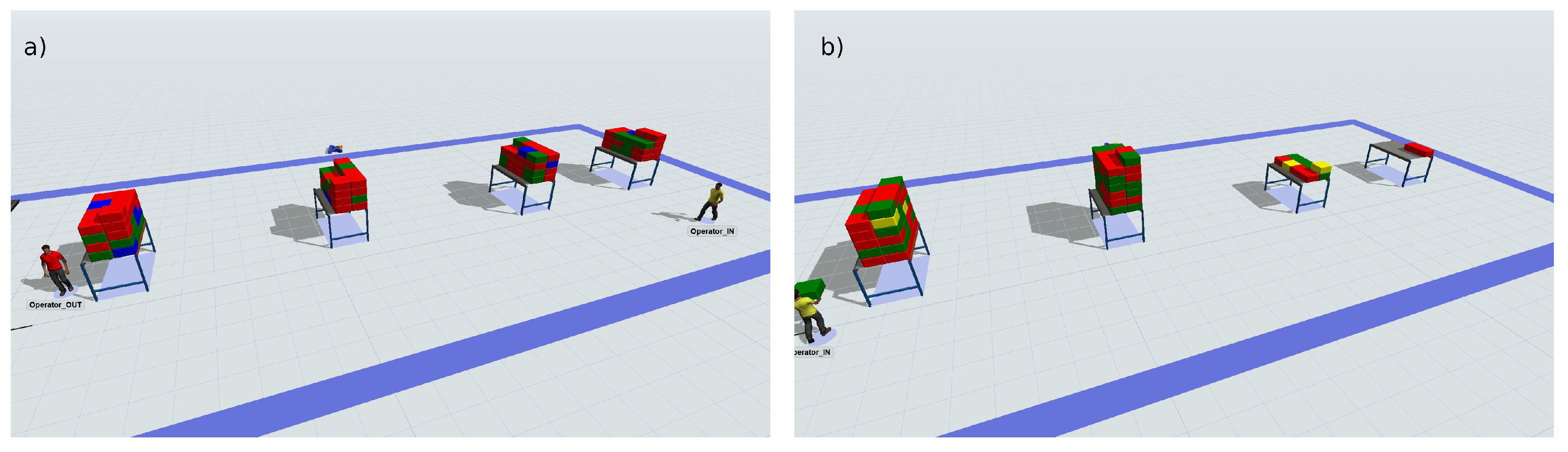
4.1. Use Case Description

The case study developed in this work is a simplified but dynamic version of a storage location assignment problem (SLAP), where items arrive at an entry point and have to be stored in different racks. In the most generic version, the goal of the SLAP is to define the optimal allocation for items in the available locations in a given warehouse, while considering the impact of this allocation on the handling cost or the storage space efficiency. The use of predefined policies (e.g., random, fixed, or class-based) is one of the most common approaches for dealing with the SLAP in a real-life warehouse context. In the version presented herein, the location assignment needs to be made upon the arrival of the items, as opposed to being predefined for the entire warehouse. This means that the problem is, in that sense, dynamic because the policy can change with time depending on the current status of the warehouse. The dynamism just described increases the difficulty of solving the SLAP, which could be arduous to solve using classic methods for warehouse optimization, such as metaheuristics. This type of dynamic problem, which requires real-time decision-making, could be potentially better addressed by employing either learnheuristics [53] or, as proposed in this paper, an RL agent that learns the policy to be applied given the status of the warehouse and the incoming items. In order to compensate for the additional difficulty of the use case problem definition, a minimalistic problem set-up will be considered, as shown in Figure 3.

Figure 3. Schematic representation of the use case (top) and screenshot of the simulation set-up (bottom). It can be seen that the positions of the input (IN) and output (OUT) points make the first storage location the most appropriate for reducing the traveled distance of the operators, if no other restriction is considered.

The available locations of the warehouse are reduced to only four locations in which the incoming products can be placed. The rate at which the items arrive to the input point is fixed, and the type of products that arrive belong to four different categories (A, B, C, and D), depending on how frequently they are received in (or shipped out from) the warehouse. The movement frequency is assigned to the items according to a certain probability distribution, in particular, items of type A arrive and are requested with a $50\%$ chance, items of type B arrive and are requested with $31\%$ probability, items type C arrive and are requested with $13\%$ probability, and items type D arrive and are requested with $6\%$ probability. Furthermore, the capacity of the racks is limited to 50 items. This implies that, given the relative position of the rack with respect to the input and output points, there are locations (racks) in the warehouse that are more convenient than others depending on the product type and the space available. Hence, the goal is to let an artificial intelligence autonomously learn what are the most convenient locations for the next arriving product given the current status of the warehouse. In order to verify if the artificial intelligence (i.e., the trained RL model) is actually learning the best possible policy, a couple of benchmark policies were defined. These are the random policy (Algorithm 2) and the greedy policy (Algorithm 3). In Section 4.5, the results of these policies are compared against the result from the RL framework shown in Algorithm 1.

This simplified setting has some advantages for the purposes of this work: (i) the time for training the algorithm can be reduced, since the FlexSim simulation can run to termination very quickly, allowing for more learning episodes to be employed; (ii) the number of factors influencing the evolution of the simulation is limited, so the decisions made by the RL agent can still be interpreted to a great extent by researchers and practitioners; (iii) the performance of policy obtained can be validated, given the fact that a very effective policy for this warehouse set-up is known beforehand, namely, a greedy policy; and (iv) a simple and well-defined warehouse scenario, for which the performance metric is easy to obtain, could be employed as a benchmark instance for future research efforts. On the last point, a FlexSim simulation environment could be added to a collection of environments used for validation and benchmarking of RL algorithms, such as the one available for the Python Gym library, which is presented below.

Algorithm 2 Random policy.

Input: Item, Locations  Output: Location      ▹ Location ∈ Locations to which the Item is assigned 1: while isAssigned$\left(Item\right)$$\ne \mathbf{true}$ do 2:  $k\leftarrow$ randomUniformBetween$(1,count(Locations\left)\right)$ 3:  $Location\leftarrow$ selectLocation$(Locations,k)$ 4:  if isFull$\left(Location\right)$$=\mathbf{true}$ then 5:   $Locations\leftarrow$ removeLocation$(Locations,Location)$ 6:  else 7:   $Location\leftarrow$ assignItem$(Location,Item)$ 8: return Location 9: $\mathbf{end}$

Algorithm 3 Greedy policy.

Input: Item, Locations  Output: Location 1: while isAssigned$\left(Item\right)$$\ne \mathbf{true}$ do 2:  $k\leftarrow$ minDistance$(Locations,Item)$ 3:  $Location\leftarrow$ selectLocation$(Locations,k)$ 4:  if isFull$\left(Location\right)$$=\mathbf{true}$ then 5:   $Locations\leftarrow$ removeLocation$(Locations,Location)$ 6:  else 7:   $Location\leftarrow$ assignItem$(Location,Item)$ 8: return Location 9: $\mathbf{end}$

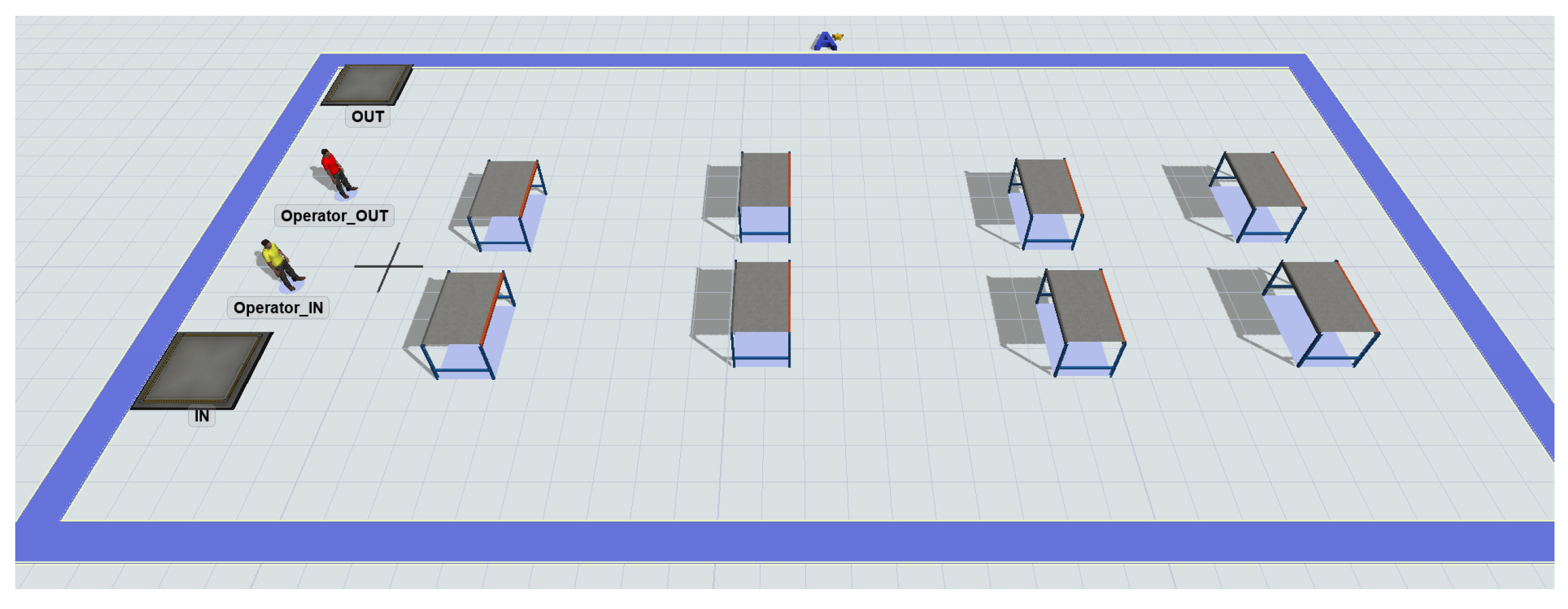
4.2. Simulation Environment

In Figure 2 and in Algorithm 1, how the classical RL loop (action–state–reward) was embedded in a communication framework between the Python RL algorithm and the FlexSim environment is shown. The simulation model contained two pickers, one dedicated to the input activity and one dedicated to the output activity. Given that only one product is picked during each travel, there is no requirement for a specific routing policy. Instead, the optimal route between the input or output point and the racks is determined using the $A^{*}$ algorithm, avoiding collision with the various obstacles present (namely, racks and the other worker). To prevent overcomplicating the model, the rest of the parameters, such as pickers’ average speed or processing times, were left to the FlexSim default values. As described in Section 4.1, the action to be taken by the RL agent is the warehouse location where to place the next item. This means that the action space is discrete and can take an integer value between 1 and 4, representing each one of the four racks shown in Figure 3. In order to learn from the environment, the current state of all the location are sent back as observations to the learning agent. This means that the observation space is also discrete, consisting in the integer amount of product of each type per rack. The incoming item is also sent as part of the observations. The observation of the environment status is made every time that a new item arrives (set at a fixed interval), and the information of the new item is also included in the observation, codified as an integer (type A = 1, type B = 2, etc.). Finally, the reward used for updating the RL policy is based on the distance workers need to travel within the warehouse to position and retrieve the items. The objective function or metrics used to evaluate and optimize SLAP can vary depending on the specific goals and requirements of the problem. Some common objective metrics include travel distance, retrieval time, space utilization, and handling costs. In many studies reviewed by [8], the total travel distance is commonly employed as the objective metric. Hence, in this case study, we adopt the travel distance as the reward function for our RL algorithms. In particular, the main driver for the reward is the inverse of the difference between the travelled distance in the current time step and the previous time step, so that a higher reward is obtained when the difference is smaller. Following the classical RL notation, the formula for the selected reward can be expressed as follows:

$$r_t=R(s_t,s_{t-1},a_{t-1})=\frac{C}{d(a_{t-1},s_t)-d(a_{t-1},s_{t-1})},$$

(1)

where $r_t$ is the actual reward obtained at time-step t, which is a function R that depends on the current state $s_t$, the previous action $a_{t-1}$, and previous state $s_{t-1}$. The function is calculated based on a constant C, which can be tuned to aid the learning, and the difference in total traveled distance d between current and previous state. We decided to refer the reward to the previous state and previous action in order to maintain the Markov property and to ensure that the agent is learning within a Markov Decision Process where the current state is dependent only upon the previous state and action.

4.3. Reinforcement Learning Implementations

Following the example provided by FlexSim on their web page (https://docs.flexsim.com/en/22.1/ModelLogic/ReinforcementLearning/KeyConcepts/KeyConcepts.html, accessed on 26 August 2023), the case study presented herein used the Python OpenAI Gym library [54] and the Stable-Baselines3 implementations of RL algorithms [55]. Gym is an open source Python library that provides a standard API to communicate between RL algorithms and a collection of environments which simulate various real-world situations, in this case with FlexSim. Similarly, Stable-Baselines3 is a popular open source Python library built on top of PyTorch, providing a collection of state-of-the-art RL algorithms. It is part of the Stable-Baselines project, which aims to offer reliable and well-tested implementations of various RL algorithms, making it easy for researchers and practitioners to experiment with and apply these algorithms to their specific problems. Three different RL algorithms from Stable-Baselines3 were employed in this paper: (i) Advantage Actor Critic (A2C), (ii) Proximal Policy Optimization (PPO), and (iii) Deep Q-Network (DQN) algorithms.

A2C is an on-policy reinforcement learning algorithm that combines elements of both policy gradient methods and value function approximation [56]. It involves training an actor (policy) network and a critic (value) network simultaneously. The actor is responsible for selecting actions, while the critic evaluates the value of state–action pairs. The advantage function, which represents how much better or worse an action is compared with the average action in a given state, plays a crucial role in A2C. During training, the actor network is updated using the policy gradient technique to maximize the expected cumulative reward. The critic network is updated to minimize the difference between the estimated value function and the actual cumulative reward. A2C often exhibits good sample efficiency and is relatively easy to implement compared with other algorithms. PPO is an on-policy RL algorithm that addresses some of the limitations of traditional policy gradient methods [57]. PPO optimizes the policy by iteratively updating it in a way that avoids large policy updates, which could lead to instability during training. The key idea behind PPO is to clip the objective function during optimization to prevent drastic changes in the policy. This clipping, referred to as the “surrogate objective”, ensures that the updated policy remains close to the previous one. PPO also uses multiple epochs of mini-batch updates to improve data efficiency. DQN is an off-policy Q-learning algorithm that leverages deep neural networks to approximate the Q-function, which estimates the expected cumulative reward for each state–action pair [58]. DQN introduced the idea of using deep learning to represent the Q-function, allowing it to handle high-dimensional state spaces like images. The algorithm employs an experience replay buffer to store and sample transitions from past interactions with the environment. It uses a target network with delayed updates to stabilize the training process. During training, DQN minimizes the mean squared error between the Q-value predictions and the target Q-values, which are calculated using the Bellman equation.

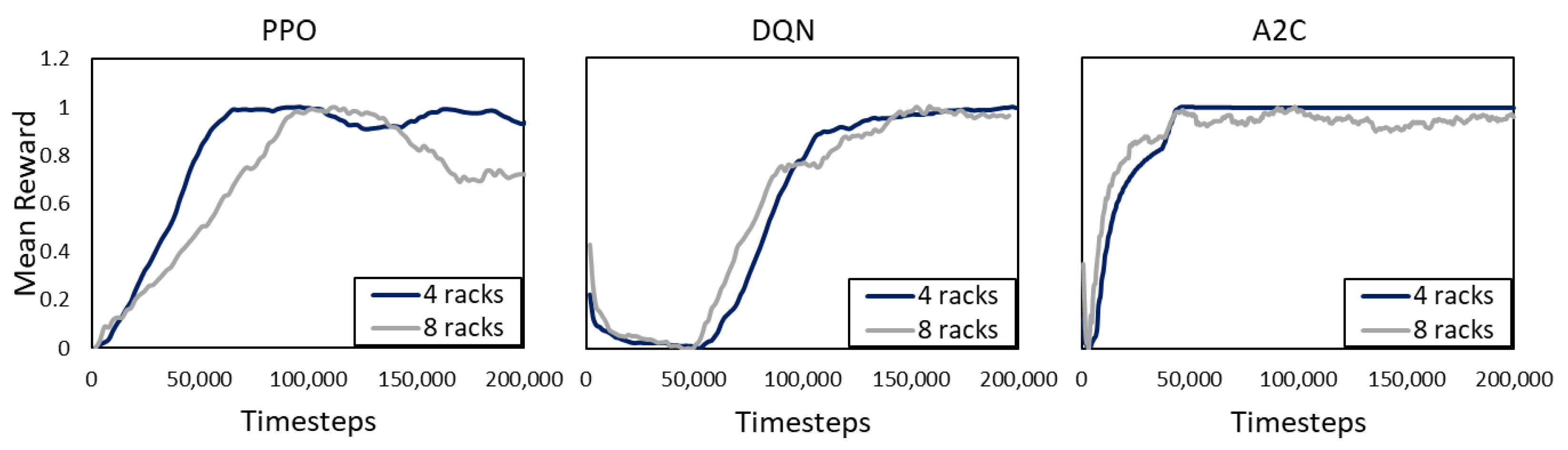
4.4. Training Results

In the current study, the total number of time steps used for training the models was fixed to 200,000, and the simulation time of FlexSim model was fixed to 5000 s. In addition, all three different RL algorithm hyperparameters were set to the default values provided via Stable-Baselines3. In fact, the hyperparameters were left unmodified since a good performance was expected with the default hyperparameter values.

Figure 4 shows the average reward obtained during the training process for three different RL algorithms, where the horizontal and vertical axes represent the timesteps of the training process and the obtained average reward, respectively. Notice that for every RL algorithm, as the training time advances, the average reward tends to increase, finally reaching an average reward of around 85. This trend indicates that the agent has learned how to place items based on the received reward, until the reward cannot be further increased. The differences in learning behavior observed among the three RL algorithms can be attributed to the underlying design and optimization strategies of the algorithms. The A2C algorithm’s behavior seems the most efficient, as in the initial phase of the training process, there is a very short descending trend in the average reward, corresponding to the exploration phase. Subsequently, as the training time advances, the average reward increases steadily, quickly reaching a plateau for the rest of the training process. Similarly, the PPO algorithm exhibits a short exploration phase in the initial training process, and as the training time advances, the average reward increases steadily. However, the average reward oscillates in the later stages of training, indicating that the PPO algorithm incorporates some exploration during the exploitation phase. In contrast, the DQN algorithm behaves somewhat differently from the other RL algorithms. The ample descending trend in the mean reward in the initial phase of the training process can be attributed to a long exploration phase, where the agent explores suboptimal actions and learns from its mistakes. Once it has collected sufficient data, the algorithm starts exploiting the learned Q-values and improves its performance. This is not surprising, as DQN is a value-based algorithm that learns to approximate the optimal Q-value function using a deep neural network. This approach generally requires more training time than A2C and PPO due to the algorithm’s need to explore the state–action space to learn the optimal Q-values.

Figure 4. Comparison of the mean reward evolution during training for three different RL algorithms using the use case simulation as environment.

4.5. Validation Results

Table 2 show the main results obtained for the use case when applying the different trained policies. The first metric evaluated is simply the distance traveled by the operators, which is used as a reward for the learning, as explained above. The second one is the number of processed items during the time defined for each simulation episode. In order to evaluate the productivity and efficiency of a warehouse (or any production system in general), a very common metric is the throughput, which evaluates the number of items processed per unit time. This is provided as the last metric in the table, which is equivalent to the number of items since the simulation time for each episode is fixed.

Table 2. Main results of the validation use case, comparing the different benchmark policies (random and greedy) against the RL agent learned policy (PPO, DQN, and A2C).

Policy	Distance Traveled (m)	Items Processed	Throughput (Items/min)
Random	7763	172	2.06
Greedy	6680	241	2.89
PPO	6801	241	2.89
DQN	6894	241	2.89
A2C	6676	241	2.89

The random policy (see Algorithm 2) can be considered the lower bound for evaluating the learning performance of the RL algorithm. On the other hand, the greedy policy (see Algorithm 3) can be used as a reference for the performance of the RL policies. This is because, if the available space within each rack is not limited, the greedy strategy is in fact the best possible strategy: the items would be placed and retrieved from the first rack, minimizing the traveled distance. However, due to the fact that a restriction in the number of items per rack was introduced, the greedy strategy is not the best possible strategy. The reason is that placing all items in the first rack regardless of their movement class (A, B, C, and D) or the state of the racks could result in filling up the first rack and being forced to place less frequent incoming items further away, which then are to be retrieved from those far away positions. On the contrary, if some space is saved in the first rack for the less frequent items, they can be input and output directly from the first rack, reducing the overall travel distance. It can be seen that the results for the different RL policies match and, in the case of the A2C algorithm, even slightly improving those of the greedy policy. This means that the RL agents are indeed learning from the underlying structure of the problem and proposing a very competitive policy. For illustrative purposes, Figure 5 shows the graphical outputs of the simulation for the untrained (random) and the trained RL policy (PPO), so they can be compared visually. With this simple but effective use case, it is demonstrated that the use of standard RL libraries in combination with advanced simulation environments can be used for training an artificial intelligence to find efficient policies that take into account realistic conditions such as those present in a warehouse.

Figure 5. Screenshot of the result (a) when the random policy is used and (b) when the trained RL policy (PPO) is used. It can be seen that in (a) that products are stored without following an assignment logic (at random) in all four racks. In (b), most items are placed in the first two racks, resulting in a reduced overall travel distance for the operators.

4.6. Performance Discussion

In order to understand the implications of scaling up the validation use case in the algorithm’s performance, an extended simulation instance was developed as shown in Figure 6. The RL training procedure described in Algorithm 1 was undertaken using the new instance and the RL implementations already presented in Section 4.3. It can be observed that the number of racks was doubled, from four to eight racks, which could represent a more realistic warehouse instance. The rest of the elements present in the simulation were kept the same (workers, input and output points, etc.) so that the impact of the increase in warehouse size can be fairly assessed. Also, the reward function defined in Equation (1) and the RL hyperparameters (learning rates, discount factors, etc.) were kept unmodified. It is important to note that the main aim of this section is not to compare the different RL implementation to find the “best” one but, rather, to showcase what there are the differences between them and how the algorithm performance was affected by the increase in size of the validation instance.

Figure 6. Screenshot of the simulation environment considered for evaluating the performance of the RL algorithm in bigger instances. The eight racks were distributed in two rows and four columns.

The three RL implementations presented in Section 4.3 were able to learn and provide very similar result in the extended instance. This meant that the different RL algorithms “understood” the simulation environment context and maximized their expected reward in the successive training episodes until the learning rate stabilized. Nonetheless, significant differences could be observed between the three different RL implementations in terms of their learning profile, as it is shown in Figure 7, where the curves were normalized, i.e., scaled so that the values fall between 0 and 1. This adjustment was performed because the absolute value of the reward is not important (it depends on a constant and the distance covered according to Equation (1)); the critical aspect is to understand if the RL agent is learning a policy that can provide good actions that can lead to increase in reward in the following environment states. The normalization allows for comparing the learning behavior across different instances, with potentially different distances between racks. It is important to note that the computational effort is equivalent in both the validation use case (four racks) and the performance use case (eight racks) simply because the length of the training is a parameter that can be adjusted. As in the validation case (see Section 4.4), the number of timesteps for training was set to 200,000.

Figure 7. Comparison of the normalized mean reward evolution during training for the three RL algorithms in both the validation environment (four racks) and the performance environment (eight racks).

One interesting result is the fact that both the DQN and the A2C algorithms displayed a very similar training behavior in both instances, suggesting that their learning profile was not significantly affected by the increased size of the warehouse. This is very likely linked to the use of the default hyperparameters, which controls how the algorithm train and learn from the simulation environment. A noticeable difference between both instances for those RL algorithms are the “ripples” that can be observed in the eight-rack instance curves. These undulations on the curves could be interpreted as the increased difficulty that the RL agent finds to the learning in the bigger instance, i.e., finding the best rack for a given item given that the current status is not as simple due to the larger observational and action spaces and, hence, the learning progress is not as stable. On the other hand, the PPO algorithm displayed a difference in behavior between both instances. In spite of the overall shape being very similar, the PPO algorithm in the eight-rack instance presents a delay of about 50,000 timesteps, making the slope of learning progress much less steep. Also, the decrease in mean reward after reaching the plateau (signifying an exploratory phase of the training) is much deeper in the eight-rack instance for the same reasons provided for the uneven curves in the DQN and A2C algorithms. However, even if the learning curves are similar (or almost equivalent in the DQN and A2C implementations), this does not mean that the quality of the learning is the same as in the validation use case, as can be seen in Table 3.

Table 3. Main results of the extended use case, comparing the different benchmark policies (random and greedy) against the RL agent learned policy (PPO, DQN, and A2C).

Policy	Distance Traveled (m)	Items Processed	Throughput (Items/min)
Random	8813	172	2.06
Greedy	6663	241	2.89
PPO	8302	241	2.89
DQN	7084	241	2.89
A2C	8704	241	2.89

As in the validation use case (four racks), the RL agents managed to correctly allocate the incoming items, keeping the warehouse throughput at its optimal value, which is the same as the greedy heuristic (see Algorithm 3). Nonetheless, the final travelled distance is greater than that of the greedy heuristic in all cases (and, as expected, always smaller than the random heuristic), with the DQN implementation being the one that provided the best results in terms of distance. For the four-rack validation instance, the A2C implementation managed to find a policy that, while keeping the optimal throughput, also reduced the travelled distance with respect to the greedy heuristic (see Section 4.5). In the extended instance (eight racks), due to the increased observation and action space, finding such a favorable policy was much more complicated. In any case, this study demonstrates that the learning capacity is maintained for the proposed RL algorithm, even under significant modifications to the environment (i.e., doubling the number of racks). The impact in performance due to a change in the environment is not straightforward to quantify due to the number of factors involved, and the difference between different RL implementations. Furthermore, it is common practice in the RL community to treat each problem instance as a problem on its own, with the necessary parameter tuning and reward calibration to achieve a satisfactory learning. In our case, a careful comparison has been carried out by keeping all factors equal except the number of racks available (which was doubled), finding that the performance is maintained in terms of throughput, but that the travelled distance performance, measured as the difference between the algorithm result and the greedy algorithm result), dropped for all RL implementations. The greatest loss in performance was for the A2C algorithm, with a 31% reduction, followed by the PPO algorithm, with a 23% reduction. Finally, the DQN algorithm, with the use of deep neural networks and a longer exploratory phase, maintained performance, with only a 3% drop in performance.

5. Key Applications and Open Research Lines

Simulation has been increasingly used in warehouse operations. Some of the key applications include the following:

• Process Optimization: analyze and optimize various processes, such as receiving, put-away, picking, packing, and shipping. Managers can identify bottlenecks, test process changes, etc.;
• Layout and Design: design and optimize the layout, including the placement of racks, shelves, etc.;
• Resource Allocation: optimize the allocation of resources, such as labor, equipment, and space;
• Inventory Management: analyze and optimize inventory management strategies, such as reorder points, safety stock levels, and order quantities;
• Demand Forecasting: simulate demand patterns and forecast inventory requirements;
• Labor Planning and Scheduling: optimize labor planning and scheduling;
• Equipment and Automation: evaluate the impact of equipment and automation technologies, such as conveyor systems, automated guided vehicles, and robots.

The main applications of RL in warehouse operations include the following:

• Warehouse Management: optimize tasks such as inventory management, order picking, and routing;
• Autonomous Robots: train autonomous robots for tasks such as automated material handling, order fulfillment, and package sorting. Robots can learn how to navigate in complex warehouse environments, handle different types of items, and interact with other equipment and personnel;
• Resource Allocation: optimize the allocation of resources such as labor, equipment, and space;
• Energy Management: optimize energy consumption, which can have a significant impact on operational costs. For example, an agent can learn to control the usage of lighting, heating, and ventilation, based on occupancy, time of day, and other environmental factors;
• Safety and Security: for example, an agent can learn to detect and respond to safety hazards, such as obstacles in pathways, spills, or damaged equipment.

The combination of advanced simulation environments and RL represents a new field that remains to be completely explored. Here are a few promising research directions:

• Wider range of applications in warehouse operations. As manufacturing and logistics systems grow more complex and businesses seek to remain both competitive and sustainable, the increasing availability of data as well as new technologies through Industry 4.0 is expected to open up a wider range of applications in warehouse operations. This will give rise to a greater number of decision variables, objective functions, and restrictions.
• Emergence of DRL. DRL holds significant potential over traditional RL due to its ability to handle high-dimensional and complex state spaces through deep neural networks. DRL allows for more efficient and automated feature extraction, enabling the model to learn directly from raw data.
• Distributed and parallel techniques. Distributed and parallel RL can accelerate the learning process by allowing multiple agents to learn concurrently. Moreover, this approach can improve scalability, as it enables RL algorithms to handle larger and more complex state spaces. Finally, distributed and parallel RL can provide robustness and fault tolerance, as multiple agents can work in parallel, and failures or perturbations in one agent do not necessarily disrupt the entire learning process.
• Explicability. Explicability is important for building trust and acceptance of RL systems, as users may be hesitant to adopt decision-making systems that lack transparency and understanding. In addition, it can aid in understanding and diagnosing model behaviour, facilitating debugging, troubleshooting, and identifying potential biases or ethical concerns. Lastly, explicability can be crucial for compliance with regulatory requirements in domains where transparency and accountability are essential.
• Metaheuristics. Metaheuristics hold potential for various applications in RL. Firstly, they can be used for hyperparameter tuning in RL algorithms to optimize the performance of agents. Secondly, metaheuristics can be employed for policy search, where they can explore the policy space to find promising policies for RL agents. Lastly, they can aid in solving complex problems in RL with high-dimensional state and action spaces, where traditional RL algorithms may struggle, by providing effective search strategies for discovering good policies. The combination of RL with metaheuristics and simheuristics [59] is also an open challenge.

6. Conclusions

Simulation has emerged as a powerful tool for optimizing decision-making in warehouses, for instance, by analyzing and optimizing various processes, including receiving, put-away, picking, packing, and shipping. By creating virtual models of warehouses and simulating different scenarios, managers can identify bottlenecks and test process changes, among others. In particular, the combination of simulation and RL offers a flexible approach for training intelligent agents in complex and dynamic environments, while mitigating challenges associated with replicating difficult or expensive scenarios in the real world. This paper showcases the integration of the FlexSim commercial simulator and the RL OpenAI Gym library in Python. Thus, we deliberately focus on a simplified version of the SLAP to highlight the connection between both components to demonstrate its feasibility. The effectiveness of the approach is validated through a set of experiments. However, enhancing the case study to reflect more complex and realistic scenarios is crucial for its broader applicability and relevance to practical settings.

Several avenues for future research can be identified, which could be categorized into three key domains: (i) enriching the SLAP modelization to describe more realistic and large-scale problems, showing that the combination of FlexSim with RL can handle these problems efficiently to deliver good performance in real-world contexts; (ii) conducting a more extensive series of experiments to compare various scenarios; and (iii) examining the performance of different RL algorithms and conducting sensitivity analyses to explore the impact of different algorithmic parameters.

References

1. Zhang, L.; Zhou, L.; Ren, L.; Laili, Y. Modeling and Simulation in Intelligent Manufacturing. Comput. Ind. 2019, 112, 103123. [Google Scholar] [CrossRef]
2. Leon, J.F.; Li, Y.; Peyman, M.; Calvet, L.; Juan, A.A. A Discrete-Event Simheuristic for Solving a Realistic Storage Location Assignment Problem. Mathematics 2023, 11, 1577. [Google Scholar] [CrossRef]
3. Sutton, R.S.; Barto, A.G. Reinforcement Learning: An Introduction; MIT Press: Cambridge, MA, USA, 2018. [Google Scholar]
4. Yan, Y.; Chow, A.H.; Ho, C.P.; Kuo, Y.H.; Wu, Q.; Ying, C. Reinforcement Learning for Logistics and Supply Chain Management: Methodologies, State of the Art, and Future Opportunities. Transp. Res. Part E Logist. Transp. Rev. 2022, 162, 102712. [Google Scholar] [CrossRef]
5. Nordgren, W.B. FlexSim Simulation Environment. In Proceedings of the Winter Simulation Conference, San Diego, CA, USA, 8–11 December 2002; Chick, S., Sánchez, P.J., Ferrin, D., Morrice, D.J., Eds.; Institute of Electrical and Electronics Engineers, Inc.: Orem, UT, USA, 2002; pp. 250–252. [Google Scholar]
6. Van Rossum, G.; Drake, F.L. Python 3 Reference Manual; CreateSpace: Scotts Valley, CA, USA, 2009. [Google Scholar]
7. Leon, J.F.; Marone, P.; Peyman, M.; Li, Y.; Calvet, L.; Dehghanimohammadabadi, M.; Juan, A.A. A Tutorial on Combining Flexsim With Python for Developing Discrete-Event Simheuristics. In Proceedings of the 2022 Winter Simulation Conference (WSC), Singapore, 11–14 December 2022; Institute of Electrical and Electronics Engineers, Inc.: Singapore, 2022; pp. 1386–1400. [Google Scholar]
8. Reyes, J.; Solano-Charris, E.; Montoya-Torres, J. The Storage Location Assignment Problem: A Literature Review. Int. J. Ind. Eng. Comput. 2019, 10, 199–224. [Google Scholar] [CrossRef]
9. Kinoshita, M.; Watanabe, M.; Kawakami, T.; Kakazu, Y. Emergence of field intelligence for autonomous block agents in the automatic warehouse. Intell. Eng. Syst. Through Artif. Neural Netw. 1999, 9, 1129–1134. [Google Scholar]
10. Rao, J.J.; Ravulapati, K.K.; Das, T.K. A simulation-based approach to study stochastic inventory-planning games. Int. J. Syst. Sci. 2003, 34, 717–730. [Google Scholar] [CrossRef]
11. Yan, W.; Lin, C.; Pang, S. The Optimized Reinforcement Learning Approach to Run-Time Scheduling in Data Center. In Proceedings of the 2010 Ninth International Conference on Grid and Cloud Computing, Nanjing, China, 1–5 November 2010; pp. 46–51. [Google Scholar]
12. Estanjini, R.M.; Li, K.; Paschalidis, I.C. A least squares temporal difference actor-critic algorithm with applications to warehouse management. Nav. Res. Logist. 2012, 59, 197–211. [Google Scholar] [CrossRef]
13. Dou, J.; Chen, C.; Yang, P. Genetic Scheduling and Reinforcement Learning in Multirobot Systems for Intelligent Warehouses. Math. Probl. Eng. 2015, 2015. [Google Scholar] [CrossRef]
14. Rabe, M.; Dross, F. A reinforcement learning approach for a decision support system for logistics networks. In Proceedings of the 2015 Winter Simulation Conference (WSC), Huntington Beach, CA, USA, 6–9 December 2015; pp. 2020–2032. [Google Scholar]
15. Wang, Z.; Chen, C.; Li, H.X.; Dong, D.; Tarn, T.J. A novel incremental learning scheme for reinforcement learning in dynamic environments. In Proceedings of the 2016 12th World Congress on Intelligent Control and Automation (WCICA), Guilin, China, 12–15 June 2016; pp. 2426–2431. [Google Scholar]
16. Drakaki, M.; Tzionas, P. Manufacturing scheduling using Colored Petri Nets and reinforcement learning. Appl. Sci. 2017, 7, 136. [Google Scholar] [CrossRef]
17. Kono, H.; Katayama, R.; Takakuwa, Y.; Wen, W.; Suzuki, T. Activation and spreading sequence for spreading activation policy selection method in transfer reinforcement learning. Int. J. Adv. Comput. Sci. Appl. 2019, 10, 7–16. [Google Scholar] [CrossRef][Green Version]
18. Li, M.P.; Sankaran, P.; Kuhl, M.E.; Ganguly, A.; Kwasinski, A.; Ptucha, R. Simulation analysis of a deep reinforcement learning approach for task selection by autonomous material handling vehicles. In Proceedings of the 2018 Winter Simulation Conference (WSC), Gothenburg, Sweden, 9–12 December 2018; pp. 1073–1083. [Google Scholar]
19. Sartoretti, G.; Kerr, J.; Shi, Y.; Wagner, G.; Satish Kumar, T.; Koenig, S.; Choset, H. PRIMAL: Pathfinding via Reinforcement and Imitation Multi-Agent Learning. IEEE Robot. Autom. Lett. 2019, 4, 2378–2385. [Google Scholar] [CrossRef]
20. Li, M.P.; Sankaran, P.; Kuhl, M.E.; Ptucha, R.; Ganguly, A.; Kwasinski, A. Task Selection by Autonomous Mobile Robots in a Warehouse Using Deep Reinforcement Learning. In Proceedings of the 2019 Winter Simulation Conference, National Harbor, MD, USA, 8–11 December 2019; Institute of Electrical and Electronics Engineers, Inc.: National Harbor, MD, USA, 2019; pp. 680–689. [Google Scholar]
21. Barat, S.; Kumar, P.; Gajrani, M.; Khadilkar, H.; Meisheri, H.; Baniwal, V.; Kulkarni, V. Reinforcement Learning of Supply Chain Control Policy Using Closed Loop Multi-agent Simulation. In International Workshop on Multi-Agent Systems and Agent-Based Simulation; Lecture Notes in Computer Science (Including Subseries Lecture Notes in Artificial Intelligence and Lecture Notes in Bioinformatics); Springer International Publishing: Cham, Switzerland, 2020; Volume 12025 LNAI, pp. 26–38. [Google Scholar]
22. Sun, Y.; Li, H. An end-to-end reinforcement learning method for automated guided vehicle path planning. In Proceedings of the International Symposium on Artificial Intelligence and Robotics 2020, Kitakyushu, Japan, 1–10 August 2020; Volume 11574, pp. 296–310. [Google Scholar]
23. Xiao, Y.; Hoffman, J.; Xia, T.; Amato, C. Learning multi-robot decentralized macro-action-based policies via a centralized q-net. In Proceedings of the 2020 IEEE International Conference on Robotics and Automation (ICRA), Paris, France, 31 May–31 August 2020; pp. 10695–10701. [Google Scholar]
24. Yang, Y.; Juntao, L.; Lingling, P. Multi-robot path planning based on a deep reinforcement learning DQN algorithm. CAAI Trans. Intell. Technol. 2020, 5, 177–183. [Google Scholar] [CrossRef]
25. Ushida, Y.; Razan, H.; Sakuma, T.; Kato, S. Policy Transfer from Simulation to Real World for Autonomous Control of an Omni Wheel Robot. In Proceedings of the 2020 IEEE 9th Global Conference on Consumer Electronics (GCCE), Kobe, Japan, 13–16 October 2020; pp. 952–953. [Google Scholar]
26. Shen, G.; Ma, R.; Tang, Z.; Chang, L. A deep reinforcement learning algorithm for warehousing multi-agv path planning. In Proceedings of the 2021 International Conference on Networking, Communications and Information Technology (NetCIT), Manchester, UK, 26–27 December 2021; pp. 421–429. [Google Scholar]
27. Newaz, A.A.R.; Alam, T. Hierarchical Task and Motion Planning through Deep Reinforcement Learning. In Proceedings of the 2021 Fifth IEEE International Conference on Robotic Computing (IRC), Taichung, Taiwan, 5–17 November 2021; pp. 100–105. [Google Scholar]
28. Peyas, I.S.; Hasan, Z.; Tushar, M.R.R.; Musabbir, A.; Azni, R.M.; Siddique, S. Autonomous Warehouse Robot using Deep Q-Learning. In Proceedings of the TENCON 2021–2021 IEEE Region 10 Conference (TENCON), Auckland, New Zealand, 7–10 December 2021; pp. 857–862. [Google Scholar]
29. Ha, W.Y.; Cui, L.; Jiang, Z.P. A Warehouse Scheduling Using Genetic Algorithm and Collision Index. In Proceedings of the 2021 20th International Conference on Advanced Robotics (ICAR), Ljubljana, Slovenia, 6–10 December 2021; pp. 318–323. [Google Scholar]
30. Liu, S.; Wen, L.; Cui, J.; Yang, X.; Cao, J.; Liu, Y. Moving Forward in Formation: A Decentralized Hierarchical Learning Approach to Multi-Agent Moving Together. In Proceedings of the 2021 IEEE/RSJ International Conference on Intelligent Robots and Systems (IROS), Prague, Czech Republic, 27 September–1 October 2021; pp. 4777–4784. [Google Scholar]
31. Ushida, Y.; Razan, H.; Sakuma, T.; Kato, S. Omnidirectional Mobile Robot Path Finding Using Deep Deterministic Policy Gradient for Real Robot Control. In Proceedings of the 2021 IEEE 10th Global Conference on Consumer Electronics (GCCE), Kyoto, Japan, 12–15 October 2021; pp. 555–556. [Google Scholar]
32. Lee, H.; Jeong, J. Mobile Robot Path Optimization Technique Based on Reinforcement Learning Algorithm in Warehouse Environment. Appl. Sci. 2021, 11, 1209. [Google Scholar] [CrossRef]
33. Tang, H.; Wang, A.; Xue, F.; Yang, J.; Cao, Y. A Novel Hierarchical Soft Actor-Critic Algorithm for Multi-Logistics Robots Task Allocation. IEEE Access 2021, 9, 42568–42582. [Google Scholar] [CrossRef]
34. Li, H.; Li, D.; Wong, W.E.; Zeng, D.; Zhao, M. Kubernetes virtual warehouse placement based on reinforcement learning. Int. J. Perform. Eng. 2021, 17, 579–588. [Google Scholar]
35. Ren, J.; Huang, X. Potential Fields Guided Deep Reinforcement Learning for Optimal Path Planning in a Warehouse. In Proceedings of the 2021 IEEE 7th International Conference on Control Science and Systems Engineering (ICCSSE), Qingdao, China, 30 July–1 August 2021; pp. 257–261. [Google Scholar]
36. Balachandran, A.; Lal, A.; Sreedharan, P. Autonomous Navigation of an AMR using Deep Reinforcement Learning in a Warehouse Environment. In Proceedings of the 2022 IEEE 2nd Mysore Sub Section International Conference (MysuruCon), Mysuru, India, 16–17 October 2022; pp. 1–5. [Google Scholar]
37. Arslan, B.; Ekren, B.Y. Transaction selection policy in tier-to-tier SBSRS by using Deep Q-Learning. Int. J. Prod. Res. 2022. [Google Scholar] [CrossRef]
38. Lewis, T.; Ibarra, A.; Jamshidi, M. Object Detection-Based Reinforcement Learning for Autonomous Point-to-Point Navigation. In Proceedings of the 2022 World Automation Congress (WAC), San Antonio, TX, USA, 11–15 October 2022; pp. 394–399. [Google Scholar]
39. Ho, T.M.; Nguyen, K.K.; Cheriet, M. Federated Deep Reinforcement Learning for Task Scheduling in Heterogeneous Autonomous Robotic System. IEEE Trans. Autom. Sci. Eng. 2022, 1–13. [Google Scholar] [CrossRef]
40. Zhou, L.; Lin, C.; Ma, Q.; Cao, Z. A Learning-based Iterated Local Search Algorithm for Order Batching and Sequencing Problems. In Proceedings of the 2022 IEEE 18th International Conference on Automation Science and Engineering (CASE), Mexico City, Mexico, 20–24 August 2022; pp. 1741–1746. [Google Scholar]
41. Cestero, J.; Quartulli, M.; Metelli, A.M.; Restelli, M. Storehouse: A reinforcement learning environment for optimizing warehouse management. In Proceedings of the 2022 International Joint Conference on Neural Networks (IJCNN), Padua, Italy, 18–23 July 2022; pp. 1–9. [Google Scholar]
42. Choi, H.B.; Kim, J.B.; Han, Y.H.; Oh, S.W.; Kim, K. MARL-Based Cooperative Multi-AGV Control in Warehouse Systems. IEEE Access 2022, 10, 100478–100488. [Google Scholar] [CrossRef]
43. Elkunchwar, N.; Iyer, V.; Anderson, M.; Balasubramanian, K.; Noe, J.; Talwekar, Y.; Fuller, S. Bio-inspired source seeking and obstacle avoidance on a palm-sized drone. In Proceedings of the 2022 International Conference on Unmanned Aircraft Systems (ICUAS), Dubrovnik, Croatia, 21–24 June 2022; pp. 282–289. [Google Scholar]
44. Wang, D.; Jiang, J.; Ma, R.; Shen, G. Research on Hybrid Real-Time Picking Routing Optimization Based on Multiple Picking Stations. Math. Probl. Eng. 2022, 2022, 5510749. [Google Scholar] [CrossRef]
45. Ekren, B.Y.; Arslan, B. A reinforcement learning approach for transaction scheduling in a shuttle-based storage and retrieval system. Int. Trans. Oper. Res. 2022. [Google Scholar] [CrossRef]
46. Yu, H. Research on Fresh Product Logistics Transportation Scheduling Based on Deep Reinforcement Learning. Sci. Program. 2022, 2022, 8750580. [Google Scholar] [CrossRef]
47. Sun, S.; Zhou, J.; Wen, J.; Wei, Y.; Wang, X. A DQN-based cache strategy for mobile edge networks. Comput. Mater. Contin. 2022, 71, 3277–3291. [Google Scholar] [CrossRef]
48. Ushida, Y.; Razan, H.; Ishizuya, S.; Sakuma, T.; Kato, S. Using sim-to-real transfer learning to close gaps between simulation and real environments through reinforcement learning. Artif. Life Robot. 2022, 27, 130–136. [Google Scholar] [CrossRef]
49. Lee, H.; Hong, J.; Jeong, J. MARL-Based Dual Reward Model on Segmented Actions for Multiple Mobile Robots in Automated Warehouse Environment. Appl. Sci. 2022, 12, 4703. [Google Scholar] [CrossRef]
50. Liang, F.; Yu, W.; Liu, X.; Griffith, D.; Golmie, N. Toward Deep Q-Network-Based Resource Allocation in Industrial Internet of Things. IEEE Internet Things J. 2022, 9, 9138–9150. [Google Scholar] [CrossRef]
51. Guo, W.; Li, S. Intelligent Path Planning for AGV-UAV Transportation in 6G Smart Warehouse. Mob. Inf. Syst. 2023, 2023, 4916127. [Google Scholar] [CrossRef]
52. Yan, Z.; Kreidieh, A.R.; Vinitsky, E.; Bayen, A.M.; Wu, C. Unified Automatic Control of Vehicular Systems with Reinforcement Learning. IEEE Trans. Autom. Sci. Eng. 2023, 20, 789–804. [Google Scholar] [CrossRef]
53. Bayliss, C.; Juan, A.A.; Currie, C.S.; Panadero, J. A Learnheuristic Approach for the Team Orienteering Problem with Aerial Drone Motion Constraints. Appl. Soft Comput. 2020, 92, 106280. [Google Scholar] [CrossRef]
54. Beysolow, T., II. Applied Reinforcement Learning with Python: With OpenAI Gym, Tensorflow, and Keras; Apress: New York, NY, USA, 2019. [Google Scholar]
55. Raffin, A.; Hill, A.; Gleave, A.; Kanervisto, A.; Ernestus, M.; Dormann, N. Stable-Baselines3: Reliable Reinforcement Learning Implementations. J. Mach. Learn. Res. 2021, 22, 1–8. [Google Scholar]
56. Mnih, V.; Badia, A.P.; Mirza, M.; Graves, A.; Lillicrap, T.; Harley, T.; Silver, D.; Kavukcuoglu, K. Asynchronous Methods for Deep Reinforcement Learning. In Proceedings of the International Conference on Machine Learning. PMLR, New York, NY, USA, 19–24 June 2016; pp. 1928–1937. [Google Scholar]
57. Schulman, J.; Wolski, F.; Dhariwal, P.; Radford, A.; Klimov, O. Proximal Policy Optimization Algorithms. arXiv 2017, arXiv:1707.06347. [Google Scholar]
58. Mnih, V.; Kavukcuoglu, K.; Silver, D.; Graves, A.; Antonoglou, I.; Wierstra, D.; Riedmiller, M. Playing Atari With Deep Reinforcement Learning. arXiv 2013, arXiv:1312.5602. [Google Scholar]
59. Rabe, M.; Deininger, M.; Juan, A.A. Speeding Up Computational Times in Simheuristics Combining Genetic Algorithms with Discrete-Event Simulation. Simul. Model. Pract. Theory 2020, 103, 102089. [Google Scholar] [CrossRef]
Disclaimer/Publisher’s Note: The statements, opinions and data contained in all publications are solely those of the individual author(s) and contributor(s) and not of MDPI and/or the editor(s). MDPI and/or the editor(s) disclaim responsibility for any injury to people or property resulting from any ideas, methods, instructions or products referred to in the content.
Article Metrics
Citations
Article Access Statistics
Multiple requests from the same IP address are counted as one view.