A Hybrid Discrete Memetic Algorithm for Solving Flow-Shop Scheduling Problems

Abstract

Flow-shop scheduling problems are classic examples of multi-resource and multi-operation scheduling problems where the objective is to minimize the makespan. Because of the high complexity and intractability of the problem, apart from some exceptional cases, there are no explicit algorithms for finding the optimal permutation in multi-machine environments. Therefore, different heuristic approaches, including evolutionary and memetic algorithms, are used to obtain the solution—or at least, a close enough approximation of the optimum. This paper proposes a novel approach: a novel combination of two rather efficient such heuristics, the discrete bacterial memetic evolutionary algorithm (DBMEA) proposed earlier by our group, and a conveniently modified heuristics, the Monte Carlo tree method. By their nested combination a new algorithm was obtained: the hybrid discrete bacterial memetic evolutionary algorithm (HDBMEA), which was extensively tested on the Taillard benchmark data set. Our results have been compared against all important other approaches published in the literature, and we found that this novel compound method produces good results overall and, in some cases, even better approximations of the optimum than any of the so far proposed solutions.

1. Introduction

Scheduling problems, in general, have been extensively studied across a wide range of domains due to their relevance for optimizing resource allocation, improving productivity, and reducing operational costs. Efficient scheduling has a direct impact on overall system performance, making it a critical area of research in operations management and industrial engineering. Flow-shop scheduling belongs to the broader class of multi-resource and multi-operation scheduling problems. With all its variants, it belongs to the class of NP-hard problems, which are known to have no polynomial time solution method. As a matter of course, small tasks or very special cases may be handled in reasonable time, but in general these problems are intractable. Obviously, the time complexity of finding a good solution in a shorter time may essentially effect the efficiency and the costs of real industrial and logistics applications. Alas, in such problems, the complexity increases exponentially in terms of the number of jobs, machines, and processing steps involved. Additionally, the presence of parallel machines and precedence constraints further complicates the optimization process. These challenges make it computationally infeasible to find optimal solutions for large-scale instances, necessitating the adoption of heuristic and metaheuristic methods. Apart from some exceptional cases, there are no explicit algorithms for finding the optimal permutation in multi-machine environments. Therefore, different heuristic approaches and evolutionary algorithms are used to calculate solutions that are close to the optimal solution. Evolutionary and population-based algorithms, inspired by the principles of natural selection and geneticsor by the behavior of groups of animals have demonstrated rather good efficiency at solving various optimization problems, including flow-shop scheduling.

In recent years, the field of metaheuristic algorithms has witnessed fast growing interest. After the “plain” evolutionary approaches, like the didactically important genetic algorithm (GA), a series of combines methods were proposed that increased the efficiency. An important step was Moscato et al.’s idea, the memetic algorithm family that applied traditional mathematical optimization techniques for local search while keeping the evolutionary method for global search where the former was nested in [1]. This idea was further developed by our group; the concept was extended to discrete problems, and various simple graph theoretic and similar exhaustive optimization techniques were applied to local search [2]. The advantage of this combination is that evolutionary techniques usually lead to good results but they are rather slow, while more classical optimization may be much faster; however, they tend to stick in local optima.

As a rather straightforward question, we started to investigate further combinations of nested search algorithms. As so far simulated annealing (SA) delivered rather good results, we did some tests with the discrete memetic algorithm we had proposed as “outer” search, and SA as “inner” search. Here, it is senseless to differentiate global and local search techniques as both heuristic algorithms could be directly applied as global searchers. Nevertheless, the result was rather promising [3], and we found that the combined hybrid metaheuristic delivered in most benchmark cases was a better approximation than either of the two, without combination.

We continued these investigations and found that the development of hybrid algorithms combining multiple optimization techniques leverages the components’ individual strengths and mitigates their weaknesses. Earlier, we established some results proving that memetic algorithms have gained prominence for their ability to incorporate problem-specific local search procedures into the evolutionary search process [4]. Even though those comparisons between various evolutionary approaches and their memetic extensions were tested on continuous benchmarks, the efficiency of the memetic extension of the bacterial evolutionary algorithm [5] presented clear advantages compared to the original GA and even compared to the rather successful particle swarm optimization, but especially the memetic extension of each proved to be much better for medium and large instances of the benchmarks.

This integration of global and local search allows for a more robust exploration of the solution space and improves the speed of finding high-quality solutions reducing the likelihood of premature convergence to local optima. As mentioned above, the term memetic algorithm was first introduced by Moscato et al. drawing inspiration from some Darwinian principles of natural evolution and Richard Dawkins’ meme concept [6]. The memes are ideas—messages broadcasted throughout the whole population via a process that, in the broad sense, can be called imitation.

The no-free-lunch theorem states that any search strategy performs the same when averaged over the set of all optimization problems [7]. If an algorithm outperforms another on some problems, then the latter one must outperform the former one on others. General purpose global search algorithms like most evolutionary algorithms perform well on a wide range of optimization problems, but they may not approximate the performance of highly specialized algorithms specially designed for a given problem. Nevertheless, the no-free-lunch principle is only true in an approximate sense. In [8], we showed that under certain conditions the balance of speed and accuracy my be optimised, and it is not to be excluded that such optima always, or at least often, exist. Some general ideas concerning this balance were given in [9]. Nevertheless, the insight of balanced advantages and disadvantages leads directly to the recommendation to extend generally (globally) applicable metaheuristics with classical application-specific (locally optimal) methods, or even heuristics, leading to more efficient problem solvers, an observation that fits well with the basic concept of applying memetic and hybrid heuristic algorithms.

Above, the GA was mentioned. The bacterial evolutionary algorithm (BEA) may be considered as its further development, where some of the operators have been changed in a way inspired by the reproduction of bacteria [10], and so the algorithm became faster and produced unambiguously better approximations [4].

Let us provide an overview of the basic algorithm. As mentioned above, the BEA model replicates the process of bacterial gene crossing as seen in the nature. This process has two essential operations: bacterial mutation and gene transfer. At the start of the algorithm, an initial random population is generated, where each bacterium represents a candidate for the solution in an encoded form. The new generation is created by using the two operations mentioned above. The individual bacteria from the second generation onward are ranked according to an objective function. Some bacteria are terminated, and some are prioritized based on their traits. This process is repeated until the termination criteria are met.

Its memetic version was first applied for continuous optimization [11]. This was an extension of the original memetic algorithm to the class of bacterial evolutionary approaches, where the BEA replaced the GA. Various benchmark tests proved that the algorithm was very effective for many other application domains for optimization tasks. Several examples showed that the BEA could be applied in various fields with success, for example, timetable creation problems, automatic data clustering [12], and determining optimal 3D structures [13] as well. The first implementations of the bacterial memetic evolutionary algorithms (BMEA) were used for finding the optimal parameters of fuzzy rule-based systems. The BMEA was later successfully extended also to discrete problems, like, among others, the flow-shop scheduling problem itself, produced considerably better efficiency for some problems. A novel hybrid algorithm version with a BEA wrapper and nested SA showed remarkably good results on numerous benchmarks [3].

As discussed above, initially, the combination of bacterial evolutionary algorithms with local search methods was proposed only for the very special aim of increasing the ability to find the optimal estimation of fuzzy rules. In the original BEA paper, mechanical, chemical, and electrical engineering problems were presented as benchmark applications. In addition, a fascinating mathematical research field, namely, solving transcendental functions, completed the list of first applications. In the first version of BMEA, where the local search method applied was the second-order gradient method, the Levenberg-Marquard [14] algorithm was tested on all these benchmarks.

The benchmark tests with the BMEA obtained better results than any former ones in the literature and outscored all other approaches used to estimate the parameters of the trapezoidal fuzzy membership functions [15]. Later, first-order gradient-based algorithms were also investigated as local search, which seemed promising [11].

In the next, the idea of BMEA was extended towards discrete problems, where gradient-based local search was replaced by traditional discrete optimization, such as exhaustive search, inbounded sub-graphs. This new family of algorithms was named discrete bacterial memetic evolutionary algorithms (DBMEA). DBMEA algorithms were first tested on vairous extensions of the travelling salesman problem and produced rather promising results. DBMEA algorithms have also been investigated on discrete permutation-based problems, where the local search methods were matching bounded discrete optimization techniques.

In a GA-based discrete memetic type approach, n-opt local search algorithms were suggested by Yamada et al. [16]. The investigations with simulations reduced the algorithms to the consecutive running 2-opt and 3-opt methods. In the case of $n\ge 4$, the computational time was too high, thus limiting the pragmatical usability of the algorithm. The 2-opt algorithm was first applied to solve various routing problems [17], where in the bounded sub-graph, two graph edges were always swapped in the local search phase. It is worth noting that 3-opt [18] is similar to the 2-opt operator; here, three edges are always deleted and replaced in a single step, which results in seven different ways to reconnect the graph, in order to find the local optimum.

In this research, another class of discrete optimization problems, the flow-shop, came to focus. Thus, in the next Section 2, the paper will give a detailed explanation of the flow-shop scheduling problem. Section 3 is a detailed survey of commonly used classic and state-of-the-art algorithms. The algorithms used by the novel HDBMEA algorithm proposed in this paper will be detailed in Section 4, Section 5 and Section 6. Section 7 deals with the results from the Taillard flow-shop benchmark set and with the comparison to relevant algorithms selected from Section 3. Section 8 extensively analyses each parameter’s impact on the HDBMEA algorithm’s scheduling performance and run-time. The result of our analysis is a chosen parameter set with which we prove the abilities of our proposed algorithm.

2. The Flow-Shop Problem

Flow-shop scheduling for manufacturing is a production planning and control technique used to optimize the sequence of operations that each job must undergo in a manufacturing facility. In a flow-shop environment, multiple machines are arranged in a specific order, and each job must pass through the same sequence of operations on these machines. The objective of flow-shop scheduling is to minimize the total time required to complete all jobs (makespan) or to achieve other performance measures such as minimizing the total completion time, total tardiness, or maximizing resource utilization. The storage buffer between machines is considered to be infinite. If the manufactured products are small in physical size, it is often easy to store them in large quantities between operations [19]. Permutation flow shop is a specific type of flow-shop scheduling problem in manufacturing where a set of jobs must undergo a predetermined sequence of operations on a series of machines. In the permutation flow shop, the order of operations for each job remains fixed throughout the entire manufacturing process. However, the order in which the jobs are processed on the machines can vary, resulting in different permutations of jobs [20].

Consider a flow-shop environment, where $N_J$ denotes the number of jobs and $N_R$ is the number of resources (machines). A given permutation $j_i,i\in \{1,2,\dots ,N_J\}$, where i is the index of the job, $p_{j_i,r}$ represents the processing times, $r\in \{1,2,\dots ,N_R\}$ is the rth resource in the manufacturing line, $S_{j_i,r}$ is the starting times of job $j_i$ on machine r, and $C_{r,j_k}$ is the completion time of job $j_k$ on resource r, has the following constraints:

A resource can only process one job at a time; therefore, the start time of the next job must be equal to or greater than the completion time of its predecessor on the same resource:

$$C_{j_i,r}\le S_{j_{i+1},r}r=1,2,\dots ,N_R;i=1,2,\dots ,N_J-1.$$

(1)

A job can only be present on one resource at a given time; therefore, the start time of the same job on the next resource must be greater then or equal to the completion time of its preceding operation:

$$C_{j_i,r}\ge C_{j_i,r+1}r=1,2,\dots ,N_R-1;i=1,2,\dots ,N_J.$$

(2)

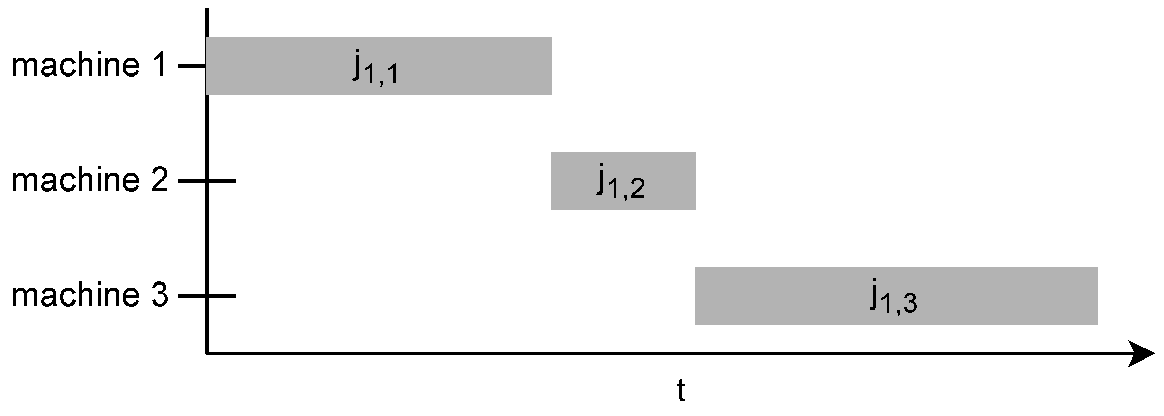
The first scheduled job does not have to wait for other jobs and is available from the start. The completion time of the first job on the current machine is the sum of its previous operations on preceding machines in the chain and its processing time on the current machine:

$$C_{j_1,r}=\sum _{k=1}^r{p}_{j_1,k}i=1,\dots ,N_R.$$

(3)

Figure 1 shows how the first scheduled job has only one contingency: its own operations on previous machines.

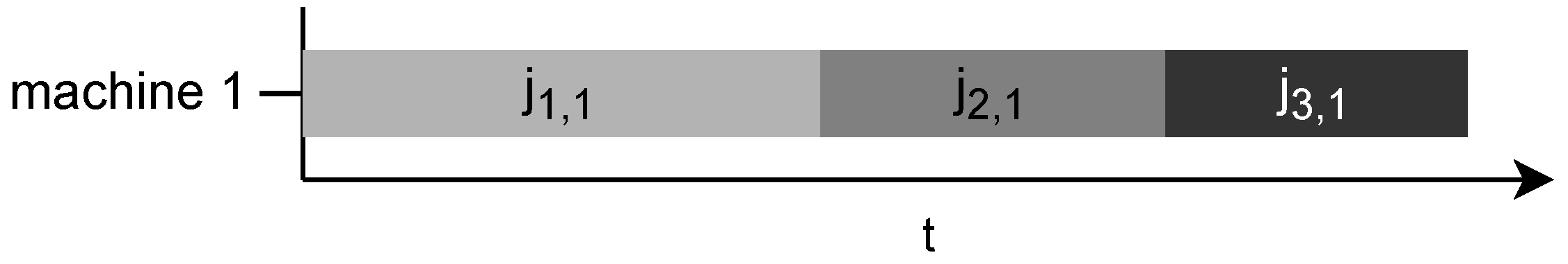
Jobs on the first resource are only contingent on jobs on the same resource; therefore, the completion time of the job is the sum of the processing times of previously scheduled jobs and its own processing time:

$$C_{j_i,1}=\sum _{k=1}^i{p}_{j_k,1}j=1,\dots ,N_J.$$

(4)

Figure 2 shows how there is only on contingency on the first machine; therefore, operations can follow each other without downtime.

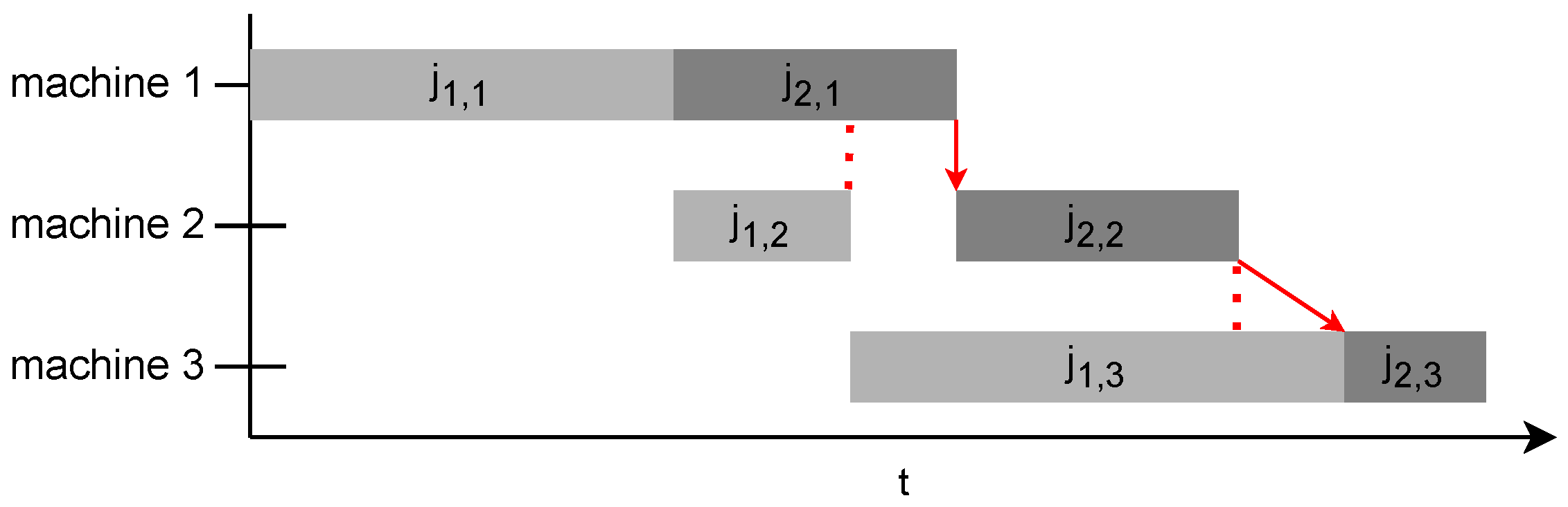
When it comes to subsequent jobs on subsequent machines, ($i>1,r>1$) the completion times depend on the same job on previous machines (Equation (2)) and previously scheduled jobs on previous machines in the chain (Equation (1)):

$$\begin{array}{c}\hfill C_{j_i,r}=max\left(C_{j_i,r-1},C_{j_{i-1},r}\right)+p_{j_i,r}\\ \hfill r=2,\dots ,N_R;i=2,\dots ,N_J.\end{array}$$

(5)

Figure 3 shows the contingency of jobs. $j_{2,2}$ is contingent upon $j_{1,2}$ and $j_{2,1}$, where it has to wait for $j_{2,1}$ to finish despite the availability of machine 2. $j_{2,3}$ is contingent upon $j_{2,2}$ and $j_{1,3}$, where it has to wait for machine 3 to become available despite being completed on machine 2.

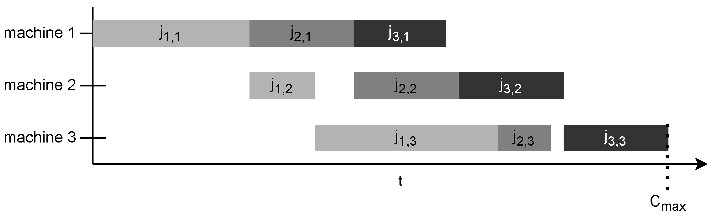
The completion time of the last job on the last resource is to be minimized and is called the makespan.

$$C_{max}=C_{j_{N_J},N_R}.$$

(6)

One of the most widely used objective function is to minimize the makespan:

$$C_{max}\to min.$$

(7)

Figure 4 illustrates how the completion time of the last scheduled job on the last machine in the manufacturing chain determines the makespan.

3. A Review of Classic and State-of-the-Art Approaches

Garey et al. proved that the flow-shop problem is NP-complete when the number of machines exceeds two [21]. Thus, massive sized problems cannot be solved by explicit mathematical algorithms. Generally, meta-heuristic search algorithms are used to traverse the search space. These algorithms are often inspired by nature incorporating metaheuristic operations into random neighborhood searches. We examined several classic and state-of-the-art algorithms, including Nawa-Enscore-Ham algorithms (Section 3.1), simulated annealing, particle swarm optimization algorithms, variable neighborhood search algorithms (Section 3.2.), genetic algorithms (Section 3.2.1), memetic algorithms (Section 3.2.2), Jaya algorithms (Section 3.2.3), and social engineering optimizers (Section 3.2.4), alongside other hybrid approaches (Section 3.2.5).

3.1. Classic Approaches

One of the most referenced algorithms is the NEHT (or NEH-Tailard) algorithm. It is based on the Nawaz–Enscore–Ham (NEH) algorithm [22] The NEH algorithm has been widely studied and used in various fields, including manufacturing, operations research, and scheduling problems. While it may not always find the optimal solution, it usually provides good-quality solutions in a reasonable amount of time, making it a practical and efficient approach for solving permutation flow-shop scheduling problems. The NEHT algorithm is improved by Taillard [23]. The NEH-Tailard algorithm works similarly to the NEH algorithm but incorporates a different way of inserting jobs into the sequence. While the original NEH algorithm used the “insertion strategy” to determine the position for each job insertion, Tailard introduced a “tie-breaking” rule to break the ties between jobs with equal makespan values during the insertion process. By carefully selecting the order of job insertion, Tailard aimed to find better solutions and potentially improve the quality of the resulting schedules. The NEH-Tailard algorithm has shown to outperform the original NEH algorithm and has been widely cited in scheduling research as a more efficient and effective approach to solving permutation flow-shop scheduling problems.

3.2. Heuristic or Meta-Heuristic Algorithms

The simulated annealing (SA) [24] algorithm is a classic pseudo-random search algorithm, inspired by the annealing process in metallurgy. It is commonly used to solve combinatorial optimization problems, especially those with a large search space and no clear gradient-based approach to finding the global optimum. The algorithm is named after the annealing process used in metallurgy, where a metal is heated to a high temperature and then gradually cooled to reduce defects and obtain a more stable crystal structure. Similarly, simulated annealing starts with a high “temperature” to allow the algorithm to explore a wide range of solutions and then gradually decreases the temperature over time to converge towards a near-optimal solution, which can produce satisfactory results for flow-shop scheduling problems [25]. The key feature of simulated annealing is the acceptance of worse solutions with decreasing probability as the temperature decreases. This enables the algorithm to explore the search space broadly in the early stages and gradually converge towards a better solution as the temperature cools down. By incorporating stochastic acceptance of worse solutions, simulated annealing is able to escape local optima and has the potential to find near-optimal solutions for complex optimization problems. There are simulated annealing based scheduling algorithms like [25,26,27,28,29,30] Particle swarm optimization (PSO) describes a group of optimization algorithms where the candidate solutions are particles that roam the search space iteratively. There are many PSO variants. The particle swarm optimization 1 (PSO1) algorithm is a PSO that uses the smallest position value (SPV) [31] heuristic approach and the VNS [32] algorithm to improve the generated permutations [33]. The particle swarm optimization 2 (PSO2) algorithm is a simple PSO algorithm proposed by Ching-Jong Liao [34]. This approach introduces a new method to transform the particle into a new permutation. The combinatorial particle swarm optimization (CPSO) algorithm improves the simple PSO algorithm to optimize for integer-based combinatorial problems. Its characteristics differ from the standard PSO algorithm in each particle’s definition and speed, and in the generation of new solutions [35]. The hybrid adaptive particle swarm optimization (HAPSO) algorithm uses an approach that optimizes every parameter of the PSO. The velocity coefficients, iteration count of the local search, upper and lower bounds of speed, and particle count are optimized during runtime, resulting in a new efficient adaptive method [36]. The PSO with expanding neighborhood topology (PSOENT) algorithm uses the neighborhood topology of a local and a global search algorithm. First, the algorithm generates two neighbours for every particle. The number of neighbours increases every iteration until it reaches the number of particles. If the termination criteria are not met, every neighbour is reinitialized. The search ends when the termination criteria are met. These steps ensure that no two consecutive iterations have identical neighbour counts. This algorithm relies on two meta-heuristic approaches: variable neighborhood search (VNS) [32] and path relinking (PR) [37,38]. VNS is used to improve the solutions of each particle, while the PR strategy improves the permutation of the best solution [39]. The ant colony optimization (ANS) [40] algorithm is a virtual ant colony-based optimization approach introduced by Marco Dorigo in 1992 [41,42]. Hayat et al., in 2023 [43], introduced a new hybridization of particle swarm optimization (HPSO) using variable neighborhood search and simulated annealing to improve search results further.

3.2.1. Approaches Based on Genetic Algorithms

The simple genetic algorithm (SGA) is a standard genetic algorithm. It is similar to the self-guided genetic algorithm (SGGA), except it is not expanded with a probability model [44]. The mining gene genetic algorithm (MGGA) was explicitly developed for scheduling resources. The linear assignment algorithm and the greedy heuristics are all built-in [44]. The artificial chromosome with genetic algorithms (ACGA) is a newfound approach. It combines an EDA (estimation of distribution approach) [45,46,47,48] with a conventional algorithm. The probability model and the genetic operator generate new solutions and differ from the SGGA [44]. The self-guided genetic algorithm (SGGA) belongs to the category of EDAs. Most EDAs use the probability model explicitly to search for new solutions without using genetic operators. They realized that global statistics and local sets of information must amend one another. The SGGA is a unique solution for combining these two types of information. It does not use a probability model but predicts each solution’s fitness. This way, the mutational and crossover operations can produce better solutions, increasing the algorithm’s efficiency [44]. Storn and Prince introduced the differential equation (DE) algorithm in 1995 [49]. Like every genetic algorithm, the DE is population-based. Floating-point-based chromosomes represent every solution. Traditional DE algorithms are unable to optimize discrete optimization problems. Therefore, they introduced the discrete differential equation (DDE) [33,50,51] algorithm, in which each solution represents a discrete permutation. In the DDE, a job’s permutation represents each individual. Since every permutation is treated stochastically, we treat every solution uniquely [51]. The genetic algorithm with variable neighborhood search (GAVNS) is a genetic algorithm that utilizes the VNS [32] local search [52]. Mehrabian and Lucas introduced the invasive weed optimization (IWO) algorithm in 2006 [53]. It is based on a common agricultural phenomenon: spreading invasive weeds. It has a straightforward, robust structure with few parameters. As a result, it is easy to comprehend and implement [54]. The hybrid genetic simulated annealing (HGSA) algorithm uses the local search capabilities of the simulated annealing (SA) algorithm and integrates it with a genetic algorithm. This way, the quality of the solutions and the runtimes are improved [55]. The hybrid genetic algorithm (HGA) differs from the simple genetic algorithm by incorporating two local search algorithms. The genetic algorithm works on the whole domain as a global search algorithm. Furthermore, it uses an orthogonal-array-based crossover (OA-crossover) to increase efficiency [56]. The hormone modulation mechanism flower pollination algorithm (HMM-FPA) is a flower pollination-based algorithm. Flowers represent each individual in the population; pollination occurs between them. They can also self-pollinate, representing closely packed flowers of the same species [57].

3.2.2. DBMEA-Based Approaches

The simple discrete bacterial memetic evolutionary algorithm (DBMEA) is a specific variant of the memetic algorithm used for optimization problems. Memetic algorithms combine elements of both evolutionary algorithms (EAs) and local search to efficiently explore the solution space and find high-quality solutions. The “Bacterial” aspect in DBMEA is inspired by the behavior of bacteria in nature. The algorithm uses a population-based approach where each candidate solution (individual) is represented as a “bacterium”. These bacteria evolve over generations using mechanisms similar to those found in evolutionary algorithms, such as selection, crossover, and mutation. The “memetic” aspect indicates that each bacterium undergoes a local search process to improve its quality within its neighborhood. This local search is typically a problem-specific optimization procedure that helps the algorithm fine-tune the solutions locally. The “discrete” in DBMEA suggests that the problem domain is discrete in nature, meaning that the variables or components of the solution are discrete and not continuous. According to our investigations, it could not generate satisfactory results based on the Taillard [23] benchmark results. Therefore, we combined it with other algorithms, producing hybrid solutions that use the DBMEA as a global search algorithm. The discrete bacterial memetic evolutionary algorithm with simulated annealing (DBMEA + SA) [3] uses the simulated annealing as a local search algorithm, while the DBMEA poses as a global search algorithm to walk the domain space similar to genetic algorithms.

3.2.3. Jaya-Based Approaches

The Jaya optimization algorithm is a parameter-less optimization technique that does not require the tuning of any specific parameters or control variables. Its simplicity and ability to strike a balance between exploration and exploitation make it effective at solving various optimization problems. It may not guarantee a global optimum, but it often converges to good-quality solutions in a reasonable amount of time for many real-world applications. In 2022, Alawad et al. [58] introduced a discrete Jaya algorithm (DJRL3M) for FSSP that improved its search results using refraction learning and three mutation methods. This method is an improvement over the discrete Jaya (DJaya) algorithm proposed by Gao et al. [59].

3.2.4. Social Engineering Optimizer

A social engineering optimizer (SEO) is described as a new single-solution meta-heuristic algorithm inspired by the social engineering (SE) phenomenon and its techniques. In SEO, each solution is treated as a counterpart to a person, and the traits of each person (e.g., one’s abilities in various fields) correspond to the variables of each solution in the search space. Ref. [60] introduces a novel sustainable distributed permutation flow-shop scheduling problem (DPFSP) based on a triple bottom line concept. A multi-objective mixed integer linear model is developed, and to handle its complexity, a multi-objective learning-based heuristic is proposed, which extends the social engineering optimizer (SEO).

3.2.5. Hybrid Approaches

In [61], the authors tackle the flow-shop scheduling problem (FSSP) on symmetric networks using a hybrid optimization technique. The study combines the strengths of ant colony algorithm (ACO) with particle swarm optimization (PSO) to create an ACO-PSO hybrid algorithm. By leveraging local control with pheromones and global maximum search through random interactions, the proposed algorithm outperforms existing ones in terms of solution quality. The ACO-PSO method demonstrates higher effectiveness, as validated through computational experiments. Addressing the NP-hard nature of flow-shop scheduling problems, ref. [62] presents a computational efficient optimization approach called NEH-NGA. The approach combines the NEH heuristic algorithm with the niche genetic algorithm (NGA). NEH is utilized to optimize the initial population, three crossover operators enhance genetic efficiency, and the niche mechanism controls population distribution. The proposed method’s application on 101 FSP benchmark instances shows significantly improved solution accuracy compared to both the NEH heuristic and standard genetic algorithm (SGA) evolutionary meta-heuristic. Ref. [63] addresses the flexible flow-shop scheduling problem with forward and reverse flow (FFSPFR) under uncertainty using the red deer algorithm (RDA). The study employs the Fuzzy Jiménez method to handle uncertainty in important parameters. The authors compare RDA with other meta-heuristic algorithms, such as the genetic algorithm (GA) and imperialist competitive algorithm (ICA). The RDA performs the best at solving the problem, achieving near-optimal solutions in a shorter time than the other algorithms.

4. Discrete Bacterial Memetic Evolutionary Algorithm (DBMEA)

The pseudo-code for the memetic algorithm is defined in Algorithm 1 [2,64]. The first step is to generate a random initial population in which each bacteria represents a solution, i.e., job sequences. The description of the algorithm uses the following notations:

• $N_{ind}$: the number of individual bacterium in the population;
• $I_{seg}$: the length of the mutation segments;
• $N_{inf}$: the number of infections in gene transfers;
• $I_{trans}$: the length of gene transfer segments;
• $x_i$: a permutation of job schedules;
• $P=\{x_1,x_2,...,x_{N_{ind}}\}$: a population consisting of permutations;
• $x^{*}$: the global best solution;
• f: the objective function;
• $N_{term}$: the termination criteria;
• $N_{notImp}$: the not improved counter;
• $N_{mutants}$: the number of mutants generated in a mutation operation.

The algorithm repeats bacterial mutation, local search, and gene transfer methods and selects the best permutation until the termination criterion is met.

4.1. Steps of the Bacterial Mutation Procedure

The bacterial mutation operates on the whole population [64]. The number of segments derives from the length of a bacterium and the length of the segment:

$$N_{seg}=⌊\frac{|P_0|}{I_{seg}}⌋$$

(8)

The number of segments equals the lower bound of a bacterium’s length divided by the segment’s length. For all of the permutations of the population, a random number $r,r\in [0;1]$ is chosen. If this random number is below the coherent segment loose rate R, the bacterium undergoes a coherent segment mutation; if it is greater than or equal to this value, the bacterium is operated on by a loose segment mutation. Each mutation algorithm is called on a bacterium $N_{seg}$ times. The segment length shifts the segments for the coherent segment mutation in each iteration. Every part of the bacterium is mutated. No shifting is needed for the loose segment mutation since its random permutation generation provides an even distribution of segments across the bacterium. The original bacterium gets overridden if the mutation algorithm generates a better alternative.

• P: the population consisting of permutations;
• $P_0$: the first bacterium of the population;
• $N_{mutants}$: the number of mutants generated for each mutation operation;
• $I_{seg}$: the length of the segment to be mutated;
• $N_{seg}$: the number of segments for each bacterium;
• R: the cohesive/loose rate;
• x: an element of P population;
• $x^{\prime }$: a mutant of x;
• f: the objective function.

Algorithm 1 Discrete bacterial memetic algorithm

P = createRandomPopulation($N_{ind}$) $x^{*}=min\{f\left(x_i\right):x_i\in P\}$ $N_{notImp}=0$ while $N_{notImp}<N_{term}$ do     $P^{\prime }$ = $bacterialMutation(P,N_{mutants},I_{seg})$     $P^{″}$ = $localSearch\left(P^{\prime }\right)$     $P^{‴}$ = $geneTransfer(P^{″},N_{inf},I_{trans})$     $x=min\{f\left(x_i\right):x_i\in P^{‴}\}$     if $x<x^{*}$ then         $x^{*}=x$     else         $N_{notImp}=N_{notImp}+1$     end if     $P=P^{‴}$ end while return$x^{*}$

Figure 5 shows how cohesive segments are chosen for mutation. The segment gets shifted across the entire bacterium without overlap. The starting index of the segment is calculated with the following equation:

$$S_{seg}=i·I_{seg}$$

(9)

The entire bacterium gets optimized locally. In Figure 5a, we see the first iteration when the iteration counter is 0. The segment starts at the first element of the permutation (index 0). Therefore, if the segment length is 3, the cohesive segment on which the algorithm operates is the first three elements of the permutation. For the next segment, the iteration counter is increased by one. Thus, the segment under mutation starts at the fourth element of the permutation (index 3). We continue this process until we run out of whole segments with $I_{seg}$ lengths. Figure 5d illustrates all the cohesive segments chosen in Algorithm 2, if $\left|x\right|=9$ and $I_{seg}=3$.

Algorithm 2 Bacterial mutation process

$N_{seg}=\lfloor \frac{|P_0|}{I_{seg}}\rfloor$ for all x in P do     $r=$ random number between 0 and 1     if $r<R$ then         for $i=0$ to $N_{seg}$ do           $S_{seg}=I_{seg}·i$           $x^{\prime }=$ coherentSegmentMutation(x, $S_{seg}$, $I_{seg}$, $N_{mutants}$)           if $f\left(x^{\prime }\right)<f\left(x\right)$ then                 $x=x^{\prime }$           end if         end for     else         for $i=0$ to $N_{seg}$ do           $x^{\prime }=$ looseSegmentMutation(x, $I_{seg}$, $N_{mutants}$)           if $f\left(x^{\prime }\right)<f\left(x\right)$ then                 $x=x^{\prime }$           end if         end for     end if end for return P

Algorithm 3 depicts the process of coherent segment mutation. This operation is applied to an individual element of the population. In total, the $N_{mutants}$ number of mutants is generated by changing the order of elements in a given coherent segment. $S_{seg}$ is the index where the segment starts. $I_{seg}$ is the length of the segment. x is the bacterium on which the mutation occurs. The first mutant has its segment reversed compared to the original. All the other variations have this segment shuffled randomly. Out of all the variations along with the original bacterium x, the best one according to the fitness function f is chosen and returned. This operation is a simple local search applied to parts of the bacterium.

• x: the bacterium to be mutated;
• $S_{seg}$: the index, where the segment starts;
• $I_{seg}$: the length of the segment;
• $x_r$: the first bacterium, where the segment is reversed;
• $x^{\prime }$: a mutated bacterium;
• f: the objective function.

Algorithm 3 Coherent segment mutation

$x_r=$ reverseSegment(x, $S_{seg}$, $S_{seg}+I_{seg}$) if $f\left(x_r\right)<f\left(x\right)$ then    $x=x_r$ end if for $i=0$ to $N_{mutants}-1$ do    $x^{\prime }=$ shuffleSegment(x, $S_{seg}$, $S_{seg}+I_{seg}$)    if $f\left(x^{\prime }\right)<f\left(x\right)$ then       $x=x^{\prime }$    end if end for return x

Figure 6 illustrates the generation of variations on a given bacterium. In the given example, the length of the permutation is $\left|x\right|=9$, the length of the segment is $I_{seg}=3$, and the starting index is $S_{seg}=0$.

The loose segment mutation operates similarly to the coherent segment mutation (Algorithm 3). The only difference is the non-cohesive segment selection. At the start of the operation, a random segment with length $I_{seg}$ is chosen from the bacterium x. The segment is first reversed to generate the first mutant. All other mutants have the selected segment shuffled randomly. According to the objective function f, the best one is chosen from all mutants and the original bacterium. Algorithm 4 defines this process.

Algorithm 4 Loose segment mutation

$S=I_{seg}$ elements from $S_{\left|x\right|}$ random permutation $V=$ array of segment values for all s of S do     $V+=x\left[s\right]$ end for for $i=0$ to $N_{mutants}$ do     $x^{\prime }=x$     if $i=0$ then         reverse(V)     else         shuffle(V)     end if     for $j=0$ to $I_{seg}$ do         $x^{\prime }\left[S\left[j\right]\right]=V\left[j\right]$     end for     if $x^{\prime }\mathrm{is}\mathrm{better}\mathrm{than}x$ then       $x=x^{\prime }$     end if end for return x

Figure 7 illustrates how a loose segment might get chosen. In the example, the length of the permutation is $\left|x\right|=9$; the segment length is $I_{seg}=3$; the random segment indexes are $S=1,3,7$; and the segment values are $V=1,8,7$. Every time the loose segment mutation operation is called, the segment is selected based on values given by a pseudo-random generator. This random selection process ensures an even distribution of segments across the bacterium. This way, non-cohesive parts of the bacterium can get optimized locally.

Figure 8 illustrates how a non-cohesive segment depicted in Figure 7 is calculated. The segment elements get reversed to generate the first mutant. The segment gets shuffled to generate all other variations until $N_{mutants}$ mutants are reached.

The coherent segment mutation operation (Algorithm 3) operates on a sequence of indexes, while the loose segment operation (Algorithm 4) breaks the sequence and samples the entire bacterium. Both operations perform a local neighborhood search on their given segment to further improve the bacterium.

4.2. Gene Transfer

The gene transfer algorithm (Algorithm 5) operates on the entire population [64]. First, the elements are sorted by their fitness values, and then the population is split in half into superior and inferior bacteria. In the next step, the gene transfer algorithm is invoked $N_{inf}$ times on a random superior and inferior bacterium. During the gene transfer process, a randomly chosen coherent segment with $I_{trans}$ length is taken from the superior bacterium and inserted into the inferior bacterium, leaving no duplicates inside the mutated permutation.

The parameters are:

• $p_{src}$: the superior source bacterium from which we choose our segment;
• $p_{dst}$: the inferior destination bacterium, into which we insert our transfer segment.

Algorithm 5 Gene transfer method

sort the population according to fitness values divide the population into superior and inferior parts for i to $N_{inf}$ do     select a random bacterium from the superior part ($p_{src}$)     select a random bacterium from the inferior part ($p_{dst}$)     select a random segment from $p_{src}$ with $I_{trans}$ length     copy the segment into $p_{dst}$ in a random position      eliminate duplicates in $p_{dst}$ end for return P

The algorithm aims to take an attribute from the better-optimized superior bacterium and transfer it to an inferior one, possibly creating a population with better fitness values. This attribute is a randomly chosen coherent segment from the superior permutation. The resulting mutated bacterium is the merge of the two input bacteria (Figure 9).

5. Monte Carlo Tree Search (MCTS) Algorithm

The Monte Carlo tree search algorithm [65] can be effectively applied to board games. It uses a search tree to model the problem: nodes represent the states of the board. Those leaves may refer to as an initial state, whose sub-leaves are the potential replies of the opponent. During the search procedure, the search tree is built using multiple steps. Each leaf stores the number of games won, and the number of total attempts, and these parameters are backpropagated to aid the traversal of the tree.

The algorithm repeats the following four steps [66]:

• Selection: starting from the root node (top-down direction), a child node is selected recursively; see (Figure 10a). When there is no unseen next node, the terminal state is reached.
• Expansion: a new random child node is added; see (Figure 10b).
• Simulation: from the new node, a simulation is performed on the problem (game), see (Figure 10c). No further child nodes are created in this step. When the terminal state is reached, the outcome of the game is evaluated as win, lose or draw (+1, −1, 0).
• Backpropagation: according to the evaluation of the simulation step, the score of the nodes is updated, moving recursively up, so that nodes store an updated statistic about games won/total number of games; see (Figure 10d).

In the selection step, the upper confidence bound (UCB) [67] Formula (10) is used to select the child node.

$$UC{B}_j=\frac{X_j}{n_j}+C·\sqrt{\frac{ln{N}_j}{n_j}},$$

(10)

where $X_j$ is the number of games won through the jth node, C is the exploration parameter that adjusts the selection strategy, $N_j$ is the number of games played through the jth parent node, and $n_j$ is the number of games played through the jth child node. The execution of the algorithm keeps asymmetrically expanding the tree; this requires balancing between exploitation and exploration steps. The constant C can be considered a weight that balances those strategies. exploitation allows the search space to be expanded randomly, and exploration reuses the bet option found.

The MCTS algorithm was initially implemented for two-person board games to solve scheduling problems. Each node represents a permutation, i.e., a possible scheduling sequence. The child nodes are created from the parent nodes by modifying operators. Each tree node is a possible solution, and the neighborhood relation exists between them. Nodes having the same solution may appear multiple times in the tree—similar to board game problems.

6. Hybrid Bacterial Memetic Algorithm

Combining multiple local search algorithms can significantly enhance the efficiency of optimization algorithms. While the original DBMEA algorithm incorporated 2-opt and 3-opt methods, these needed to be revised in some cases. This article introduces a novel hybrid approach called HDBMEA, which combines the DBMEA [2] algorithm with a modified Monte Carlo tree search (MCTS) and a simulated annealing (SA) algorithm.

The proposed HDBMEA approach achieves improved results compared to the original DBMEA [2] algorithm and other existing methods in the literature by leveraging the strengths of each of the three constituent algorithms. Specifically, MCTS enhances local search by exploring the search space more efficiently, while SA further refine the search results by effectively escaping from local optima.

To promote diversity, a mortality rate ($N_{mort}$) is also introduced, indicating the percentage of the population to be replaced by new random individuals in each iteration. Using a mortality rate ensures that the search algorithm continues exploring the search space and does not become trapped in local optima.

Overall, the proposed HDBMEA algorithm represents a promising approach to solving complex flow-shop scheduling problems, with potential applications in various domains.

7. Experimental Results

In this article, the performance of the proposed algorithm was evaluated on the Taillard benchmark problems. The upper bound solution was chosen as the basis of comparison. The quality of the results was measured as the relative signed distance from the upper bound found in the original dataset. This distance was converted to a percentage using the following formula:

$$\omega =\frac{C_{BS}-C_{UB}}{C_{UB}}·100$$

(11)

where $C_{BS}$ represents the best $C_{max}$ value found by the algorithm, $C_{UB}$ refers to the upper bound determined in the benchmark dataset, and $\omega$ indicates the goodness of the method. The lower the value is, the closer the best makespan is to the theoretical upper bound; in other words, it is the relative distance from the upper bound as a percentage. The results of the benchmark dataset, which consisted of 120 problems, are presented in

Table A1. Comparison of performance of 20 algorithms on 20 and 50 machine problems (average $\omega$).

Algorithm	Problem Size
	$\mathbf{20}\mathbf{\times }\mathbf{5}$	$\mathbf{20}\mathbf{\times }\mathbf{10}$	$\mathbf{20}\mathbf{\times }\mathbf{20}$	$\mathbf{50}\mathbf{\times }\mathbf{5}$	$\mathbf{50}\mathbf{\times }\mathbf{10}$	$\mathbf{50}\mathbf{\times }\mathbf{20}$
HAPSO [36]	0.00	0.09	0.07	0.05	2.1	3.20
PSOENT [39]	0.00	0.07	0.08	0.02	2.11	3.83
NEHT [22]	3.35	5.02	3.73	0.84	5.12	6.26
SGA [44]	1.02	1.73	1.48	0.61	2.81	3.98
MGGA [44]	0.81	1.40	1.06	0.44	2.56	3.82
ACGA [44]	1.08	1.62	1.34	0.57	2.79	3.75
SGGA [44]	1.10	1.90	1.60	1.52	2.74	3.94
DDE [49]	0.46	0.93	0.79	0.17	2.26	3.11
CPSO [33]	1.05	2.42	1.99	0.90	4.85	6.40
GMA [39,72]	1.14	2.30	2.01	0.47	3.21	4.97
PSO2 [34]	1.25	2.17	2.09	0.47	3.60	4.84
HPSO [43]	0.00	0.00	0.00	0.00	0.69	1.71
GA-VNS [52]	0.00	0.00	0.00	0.00	0.77	0.96
IWO [54]	8.69	39.51	40.44	10.87	15.85	42.21
HGSA [55]	5.89	7.35	6.48	1.14	5.40	7.66
HGA [56]	16.05	29.00	29.44	18.57	44.32	58.62
HMM-PFA [57]	20.78	31.44	32.18	19.63	44.36	58.69
DJaya [59]	0.00	0.71	1.38	0.00	1.98	2.29
DJRL3M [58]	0.00	0.65	0.24	0.00	1.96	2.28
SA [68]	0.20	0.80	0.66	2.89	0.51	3.21
MCTS + SA [65]	0.08	1.07	0.56	0.46	0.00	1.78
DBMEA + SA [3]	0.09	0.63	0.71	0.39	2.09	3.12
HDBMEA	−0.1	0.03	0.07	0.02	0.17	0.80

,

Table A2. Comparison of performance of 20 algorithms on 100, 200, and 500 machine problems (average $\omega$).

Algorithm	Problem Size
	$\mathbf{100}\mathbf{\times }\mathbf{5}$	$\mathbf{100}\mathbf{\times }\mathbf{10}$	$\mathbf{100}\mathbf{\times }\mathbf{20}$	$\mathbf{200}\mathbf{\times }\mathbf{10}$	$\mathbf{200}\mathbf{\times }\mathbf{20}$	$\mathbf{500}\mathbf{\times }\mathbf{20}$
HAPSO [36]	0.14	1.17	4.13	1.06	4.27	3.43
PSOENT [39]	0.09	1.26	4.37	1.02	4.27	2.73
NEHT [22]	0.46	2.13	5.23	1.43	4.41	2.24
SGA [44]	0.47	1.67	3.80	0.94	2.73	–
MGGA [44]	0.41	1.50	3.15	0.92	3.95	–
ACGA [44]	0.44	1.71	3.47	0.94	2.61	–
SGGA [44]	0.38	1.60	3.51	0.80	2.32	–
DDE [49]	0.08	0.94	3.24	0.55	2.61	–
CPSO [33]	0.74	2.94	7.11	2.17	6.89	–
GMA [39,72]	0.42	1.96	4.68	1.10	3.61	–
PSO2 [34]	0.35	1.78	5.13	–	–	–
HPSO [43]	0.00	0.20	0.48	0.14	1.06	0.70
GA-VNS [52]	0.00	0.08	1.31	0.11	1.17	0.63
IWO [54]	6.30	18.11	51.64	8.48	35.93	17.92
HGSA [55]	0.99	3.56	3.95	2.22	4.55	2.80
HGA [56]	19.59	44.42	70.48	46.39	81.45	52.95
HMM-PFA [57]	17.80	43.37	69.41	40.99	75.56	75.66
SA [68]	0.06	0.66	1.22	0.48	0.63	0.71
DJaya [59]	0.00	0.00	2.59	0.43	2.39	1.09
DJRL3M [58]	0.16	3.16	2.58	0.42	2.37	1.05
MCTS + SA [65]	0.14	0.98	1.12	0.61	0.65	1.00
DBMEA + SA [3]	0.33	1.36	2.91	1.32	2.83	2.16
HDBMEA	0.07	0.32	0.55	0.35	0.36	0.60

and

Table A3. Average performance ($\omega$).

Algorithm	Average $\mathit{\omega }$
HAPSO [36]	1.63
PSOENT [39]	1.65
NEHT [22]	3.35
SGA [44]	1.93
MGGA [44]	1.82
ACGA [44]	1.84
SGGA [44]	1.85
DDE [49]	1.37
CPSO [33]	3.40
GMA [39,72]	2.35
PSO2 [34]	2.40
HPSO [43]	0.48
GA-VNS [52]	0.40
IWO [54]	24.66
HGSA [55]	4.33
HGA [56]	42.61
HMM-PFA [57]	44.16
SA [68]	1.22
DJaya [59]	1.13
DJRL3M [58]	1.02
MCTS + SA [65]	0.70
DBMEA + SA [3]	1.50
HDBMEA	0.28

, respectively, where the $n\times m$ columns denote the number of jobs and resources (machines), respectively. The parameters used to obtain the results are listed in

Table 1. Parameters used for the HDBMEA algorithm.

Parameter	Value
Maximum iteration count (SA)	100
Initial temperature (SA)	300
$\alpha$ (SA)	0.1
Iteration count (MCTS)	10,000
$N_{ind}$	8
Maximum iteration count (DBMEA)	2
$N_{clones}$	8
$N_{inf}$	40
$I_{seg}$	4
$I_{trans}$	5
$N_{mort}$	0.05

, and their reasoning is detailed in Section 8.

This method allows for an easy comparison between metaheuristic algorithms. The results show that the hybrid discrete bacterial memetic evolutionary algorithm introduced by this paper provides outstanding scheduling performance regarding flow-shop problems.

8. Parameter Sensitivity Analysis

Since the proposed HDBMEA algorithm contains three distinct search algorithms, the number of parameters adds up to eleven. The determination of each parameter must be backed by an analysis. A subset of the Taillard benchmark set was used, where the number of machines and jobs equals twenty, to visualize the impact of each parameter on the overall scheduling performance and runtime. Each of the ten instances was run ten times for each parameter set (100 runs total). We considered the mean and standard deviation. The formula for obtaining the quality of each solution is detailed in Equation (11).

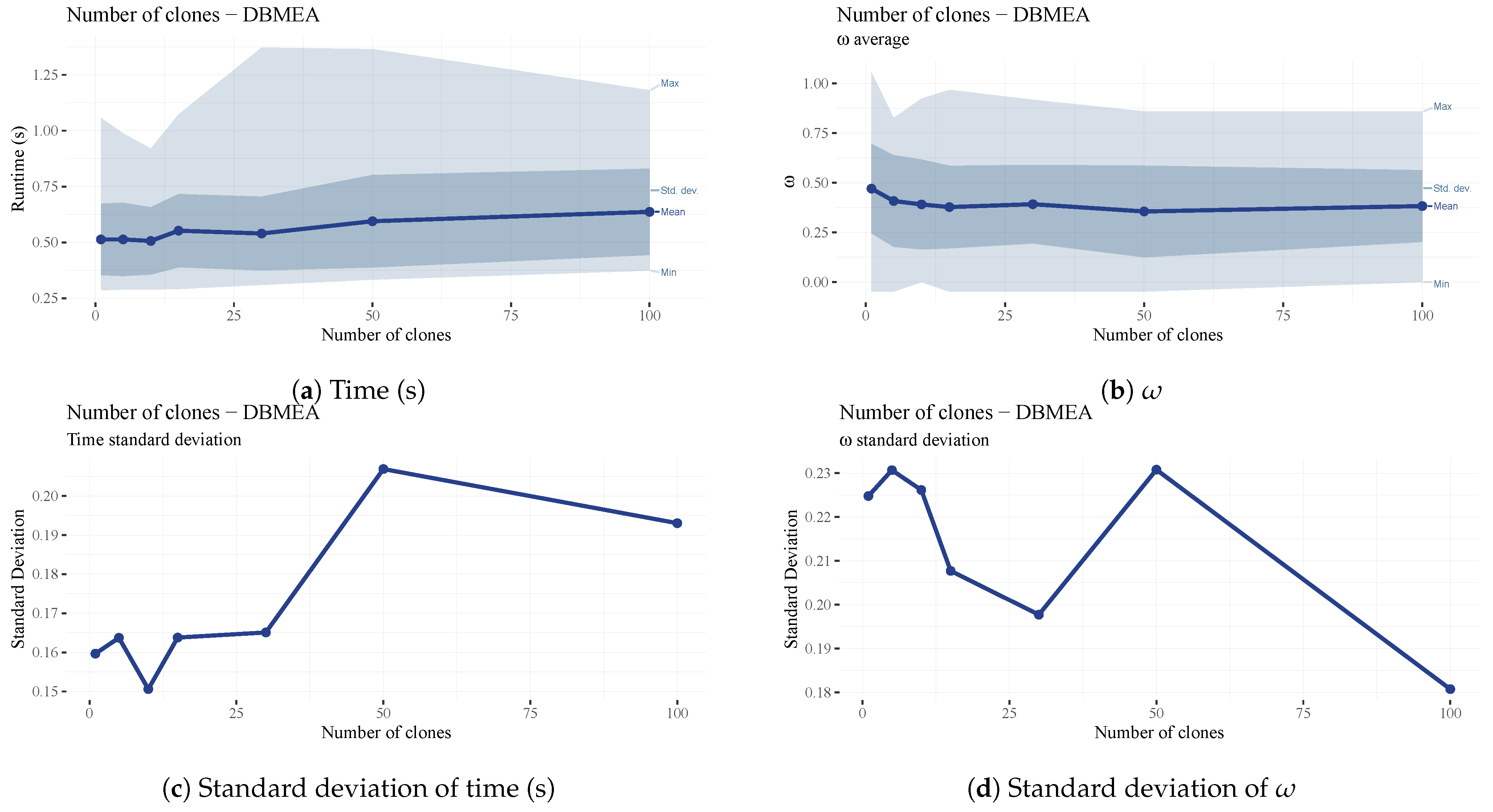
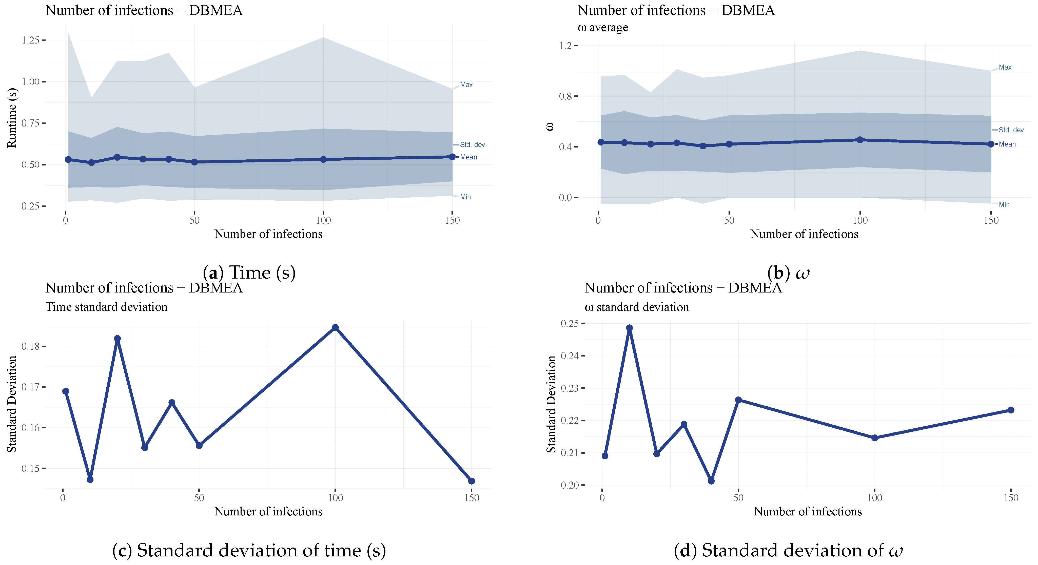
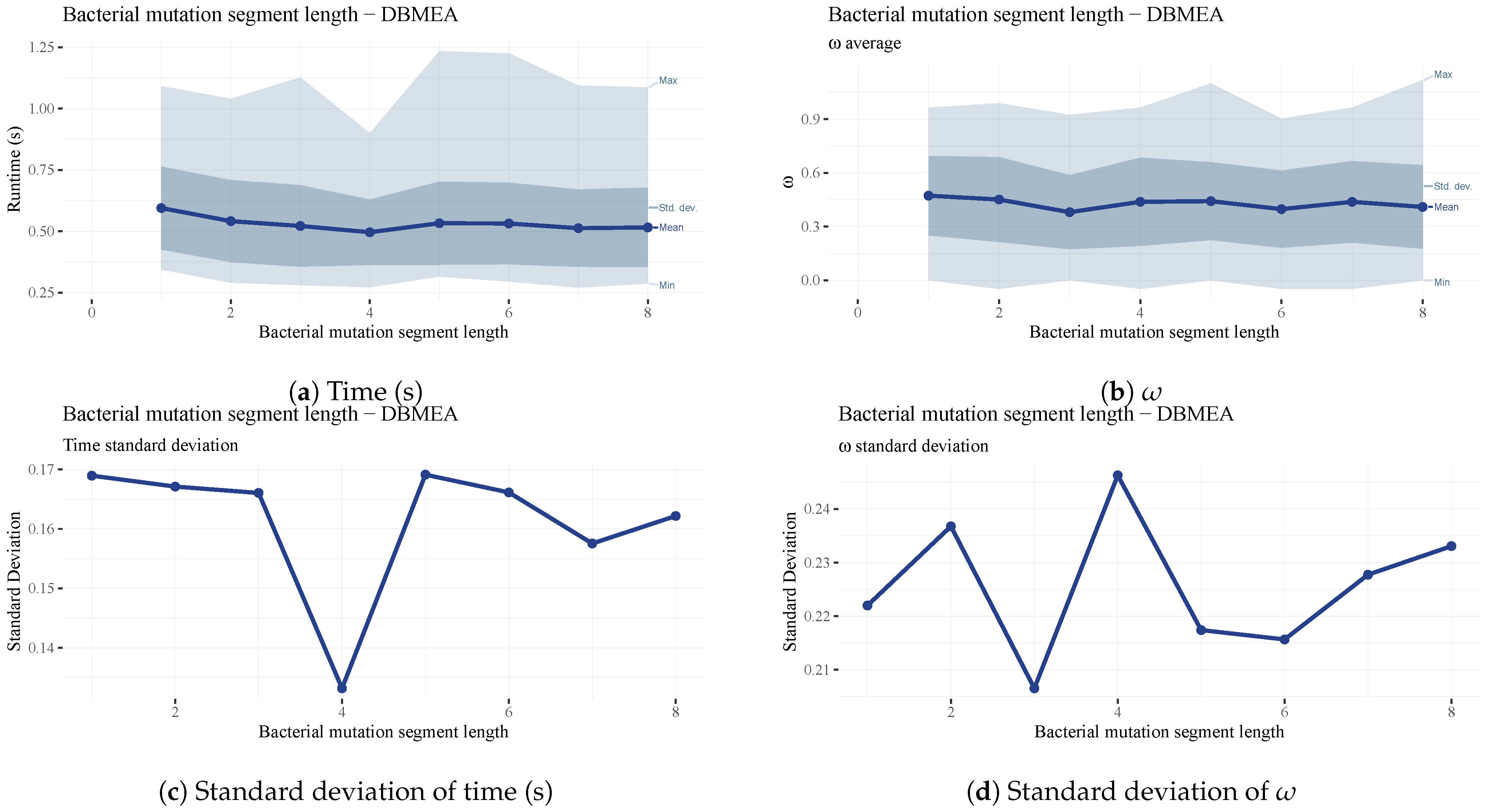
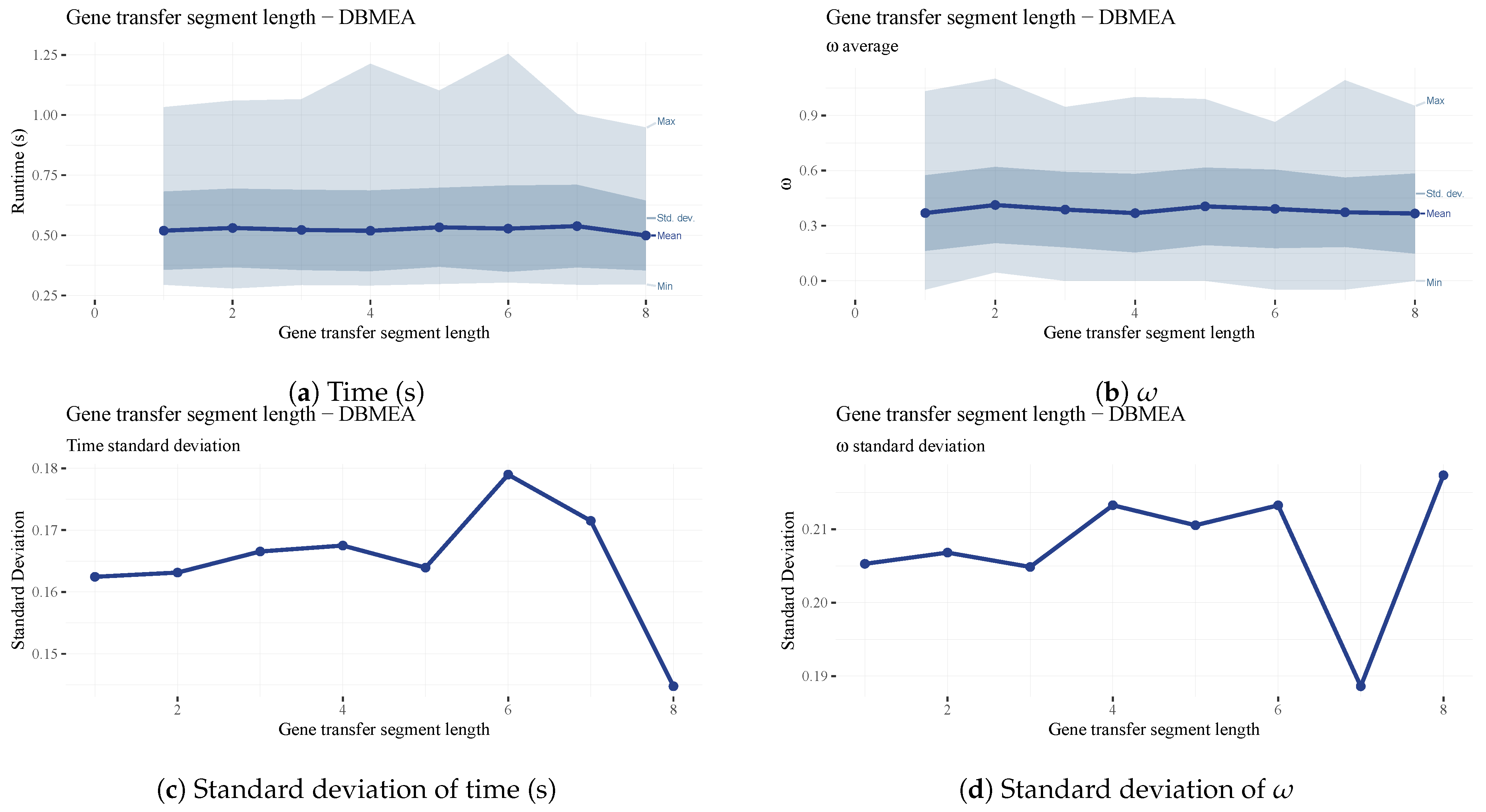
Each plot shows the overall set of values obtained (light blue ribbon), the standard deviation (mid-blue ribbon), and the mean of all runs (dark blue line). Plots showing the change in standard deviation are also included. These plots confirm our chosen set of parameters for the final benchmark results.

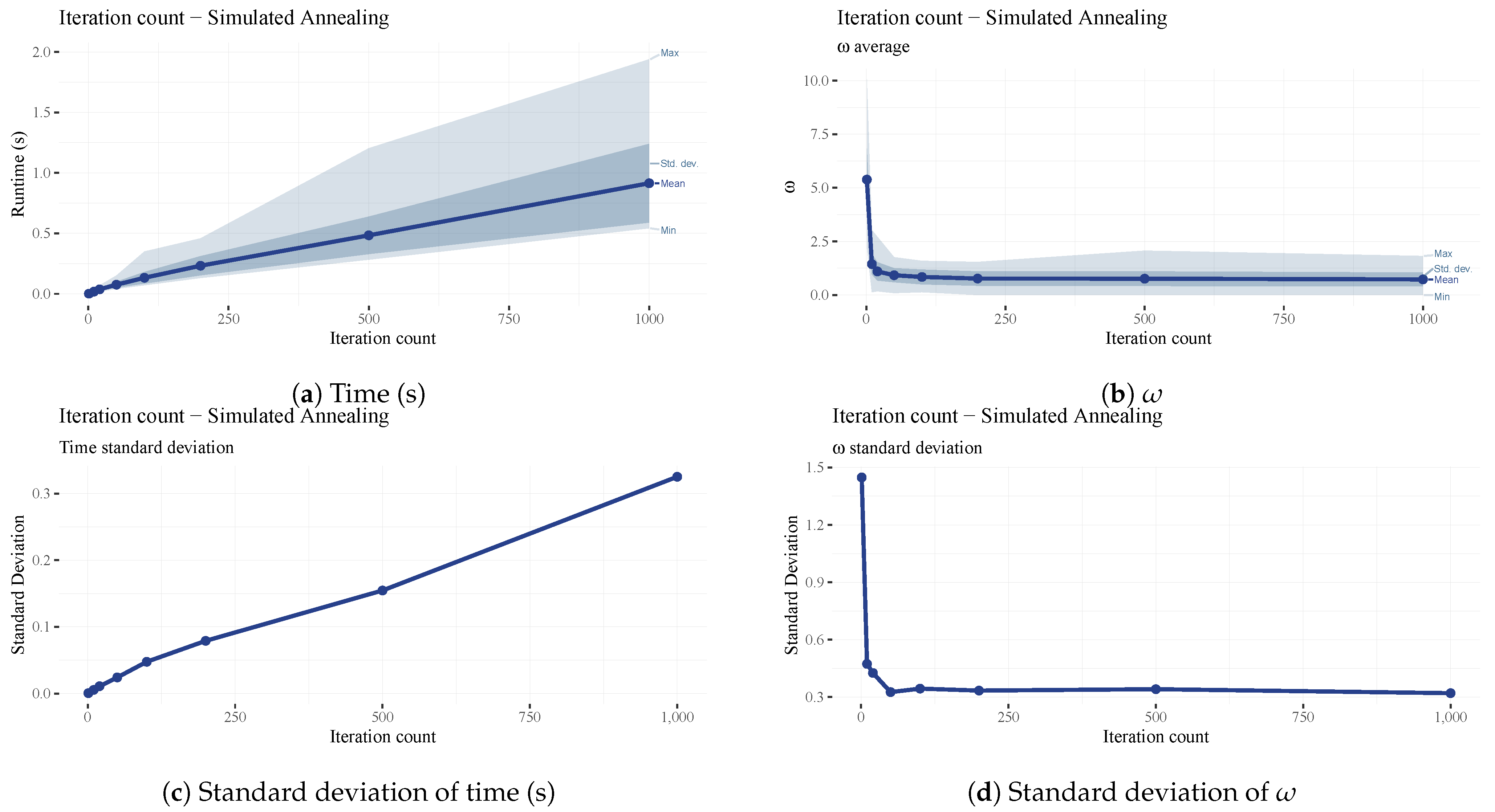
The iteration count of the simulated annealing algorithm is the maximum number of iterations since the last improvement in the makespan. This parameter dramatically impacts the results and runtime and their standard deviation (See Figure 11). The omega and standard deviation decrease dramatically until our chosen iteration count of 100 (see Figure 11b and Figure 12d), after which the improvements are negligible while the runtime keeps increasing linearly (See Figure 11a).

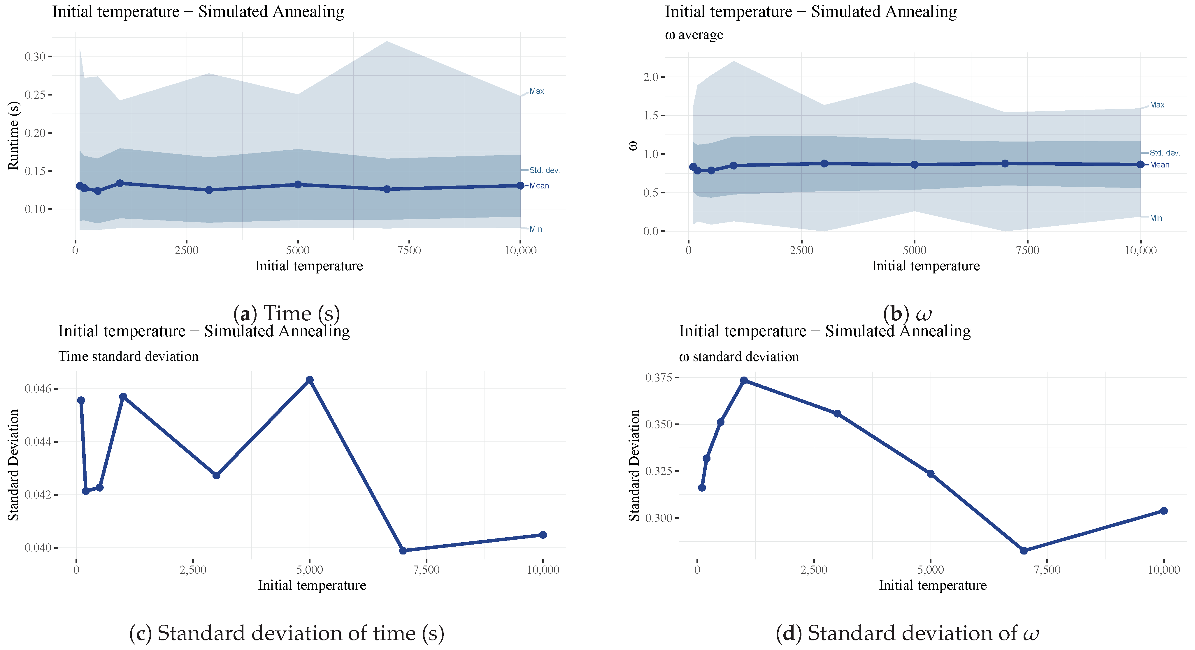
The starting temperature for the simulated annealing algorithm has little impact on the results and runtime (Figure 12); however, there is a slight dip in $\omega$ at the 300 mark (See Figure 12b), which is our chosen final value.

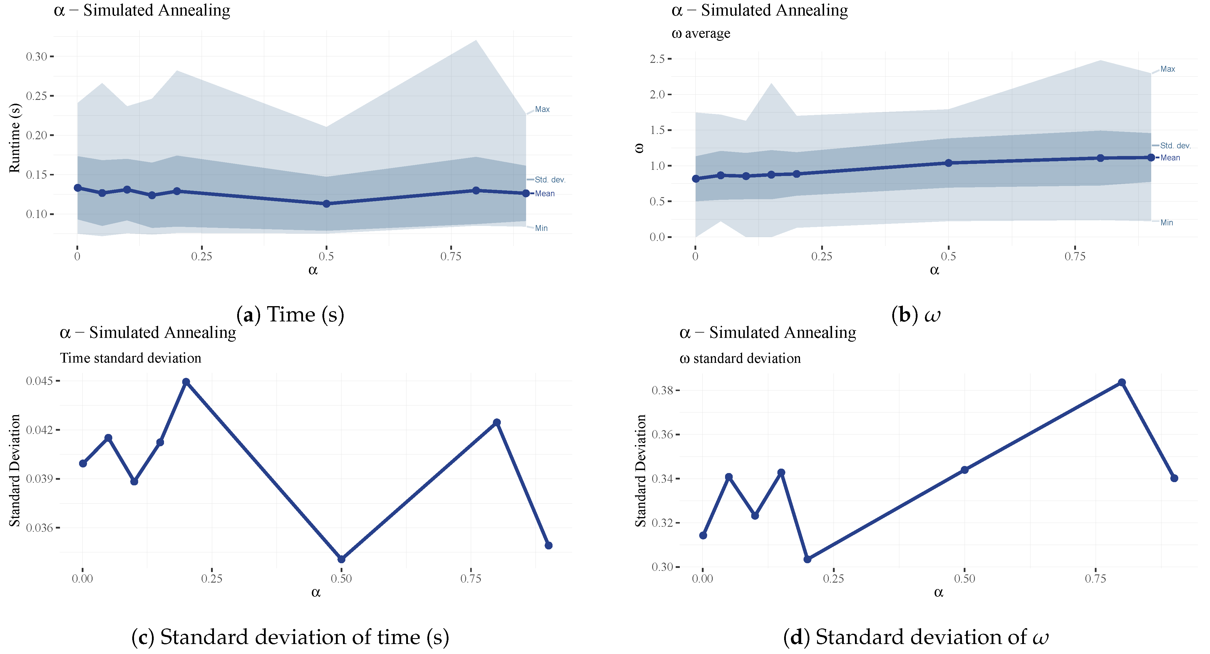
The $\alpha$ parameter of the simulated annealing algorithm is the temperature decrease in each iteration. This method creates an exponential multiplicative cooling strategy, which was proposed by Kirpatrick et al. [68], and the effects of which are considered in [69]. The parameter did not significantly affect the overall performance of the algorithm, however (Figure 13).

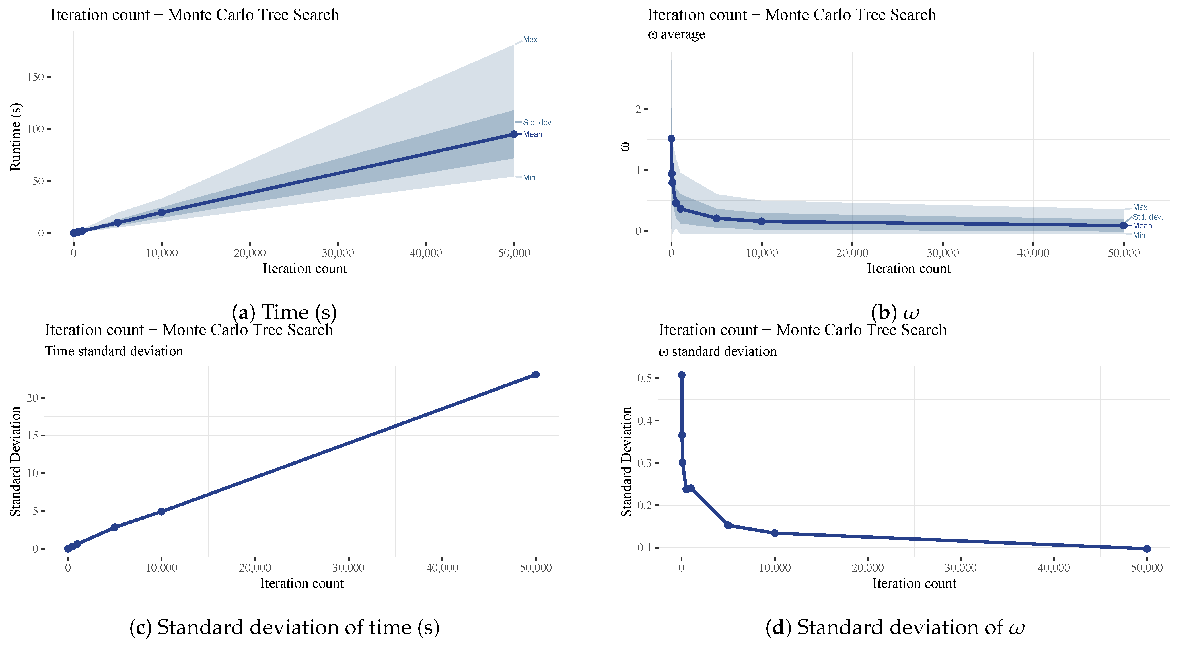
The iteration count of the MCTS algorithm is fixed; it does not take the number of iterations elapsed since the last improvement into account. This parameter improves the search results drastically (See Figure 14b), while the runtime increases only linearly (See Figure 14a). A high value of 10,000 was maintained throughout our testing since this proved to be a good middle-ground between scheduling performance ($\omega$) and runtimes. The benefit of a high iteration count is the decrease in the standard deviation of $\omega$ (See Figure 14d), meaning that the scheduling performance is increasingly less dependent on the processing times in the benchmark set. One downside of a high iteration count is the increase in the standard deviation of runtimes (See Figure 14c) since the SA algorithm is called every iteration, which has no fixed iteration count.

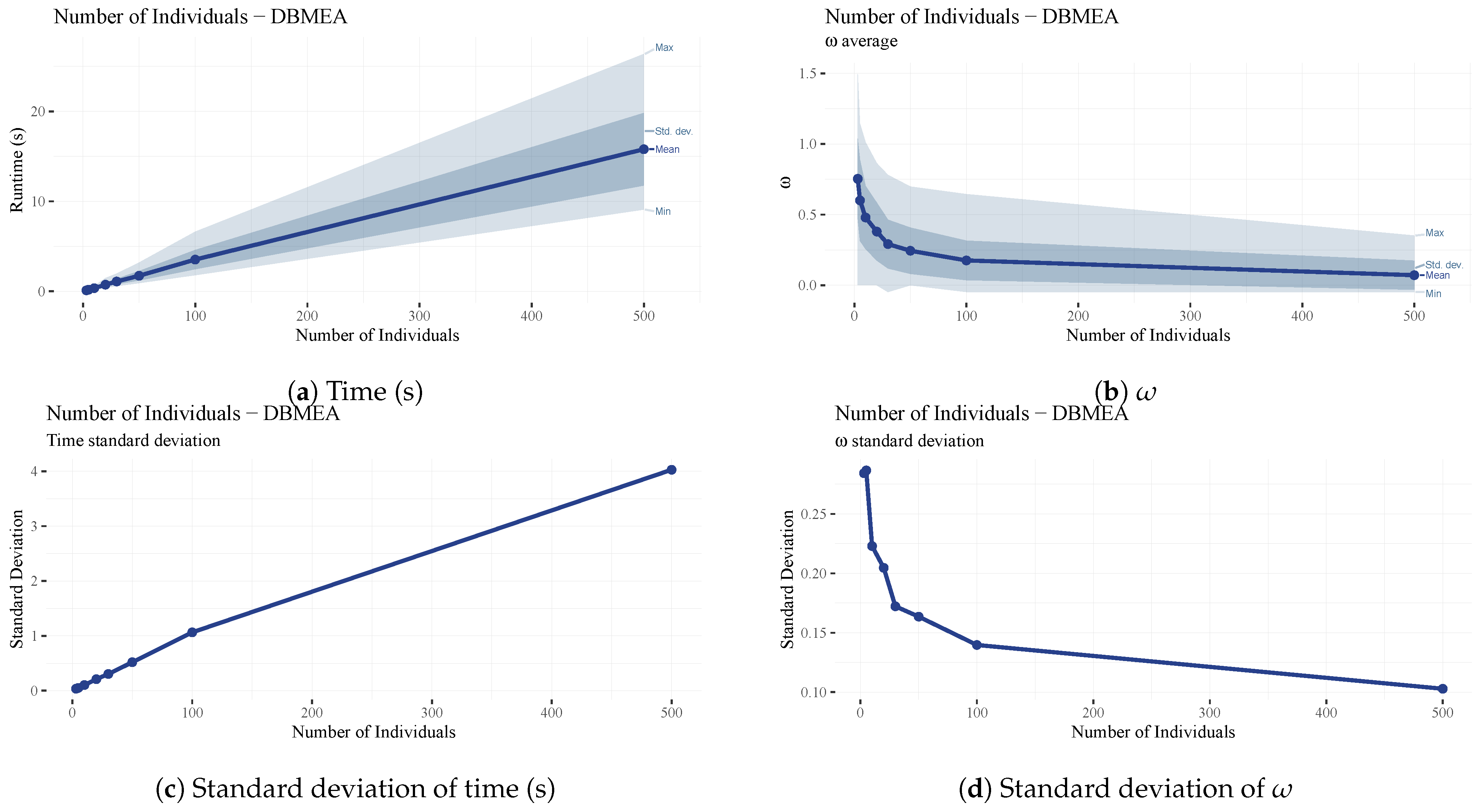
The number of individuals ($N_{ind}$) in an iteration of the Discrete Bacterial Memetic Evolutionary Algorithm (the population size) dramatically affects both the scheduling performance and the runtime (See Figure 15). A larger number of individuals means a broader range of solutions that MCTS and SA can further improve. However, a lower population count was maintained with a high iteration count in both MCTS and SA to reduce runtimes while keeping omega values low.

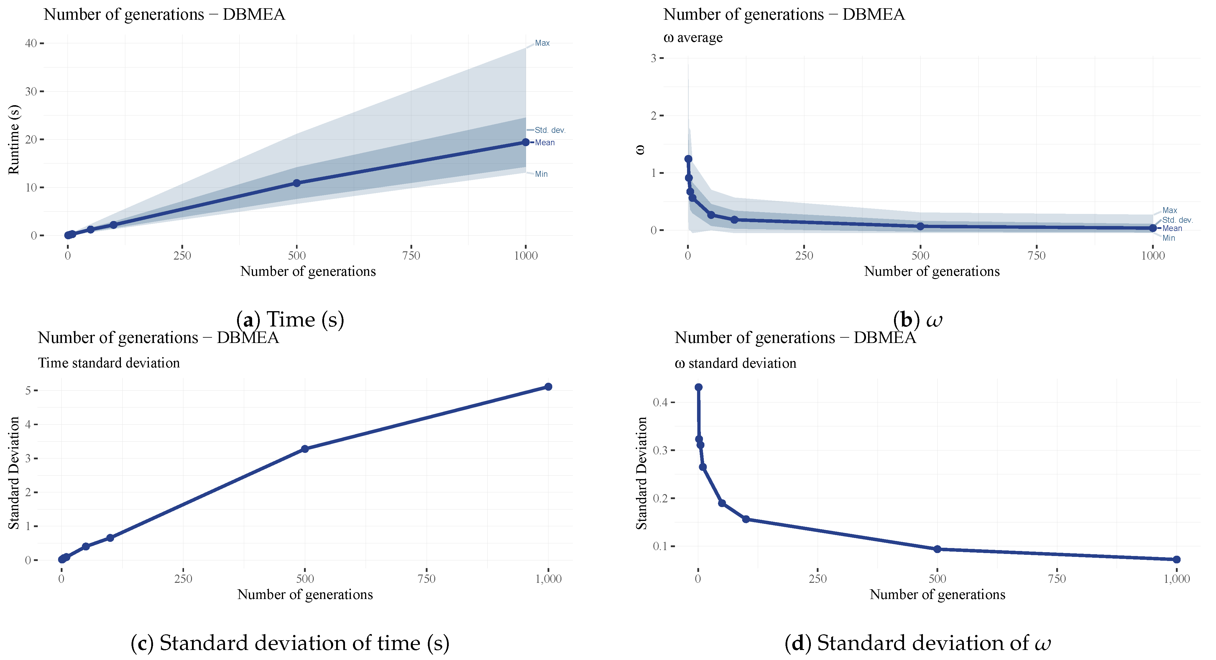
The maximum iteration count (generation count) of the DBMEA algorithm is the maximum number of iterations since the last improvement in makespan. This parameter impacts the scheduling performance and runtime significantly. $\omega$ and its standard deviation keep decreasing as the number of iterations increases (see Figure 16b,d), while the runtime is coupled linearly to the number of generations (see Figure 16a). Similarly to the population size ($N_{ind}$), the number of iterations was set to a lower value to keep MCTS and SA iteration counts high while keeping runtimes manageable.

The number of clones ($N_{clones}$) parameter is the number of clones generated in each bacterial mutation operation. An overly large number of clones creates many bacteria with the same permutation; therefore, going over a certain amount yields negligible or no improvement in overall scheduling performance (Figure 17b) while increasing runtimes (Figure 17a).

The number of infections ($N_{inf}$) is the number of new bacteria created during the gene transfer operation. This may increase diversity in the population with negligible runtime differences (See Figure 18); therefore, a higher value of forty was chosen to increase the chances of escaping local optima when scheduling larger problems.

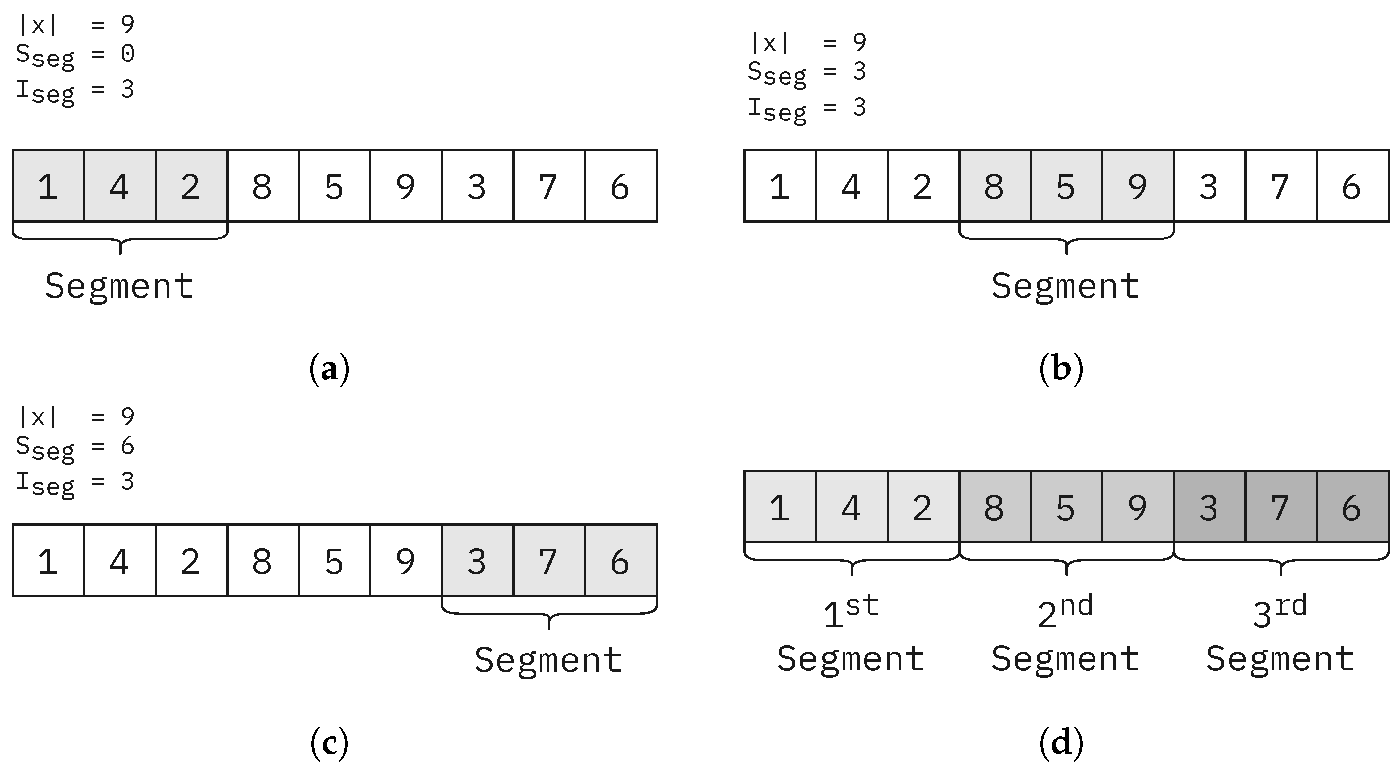
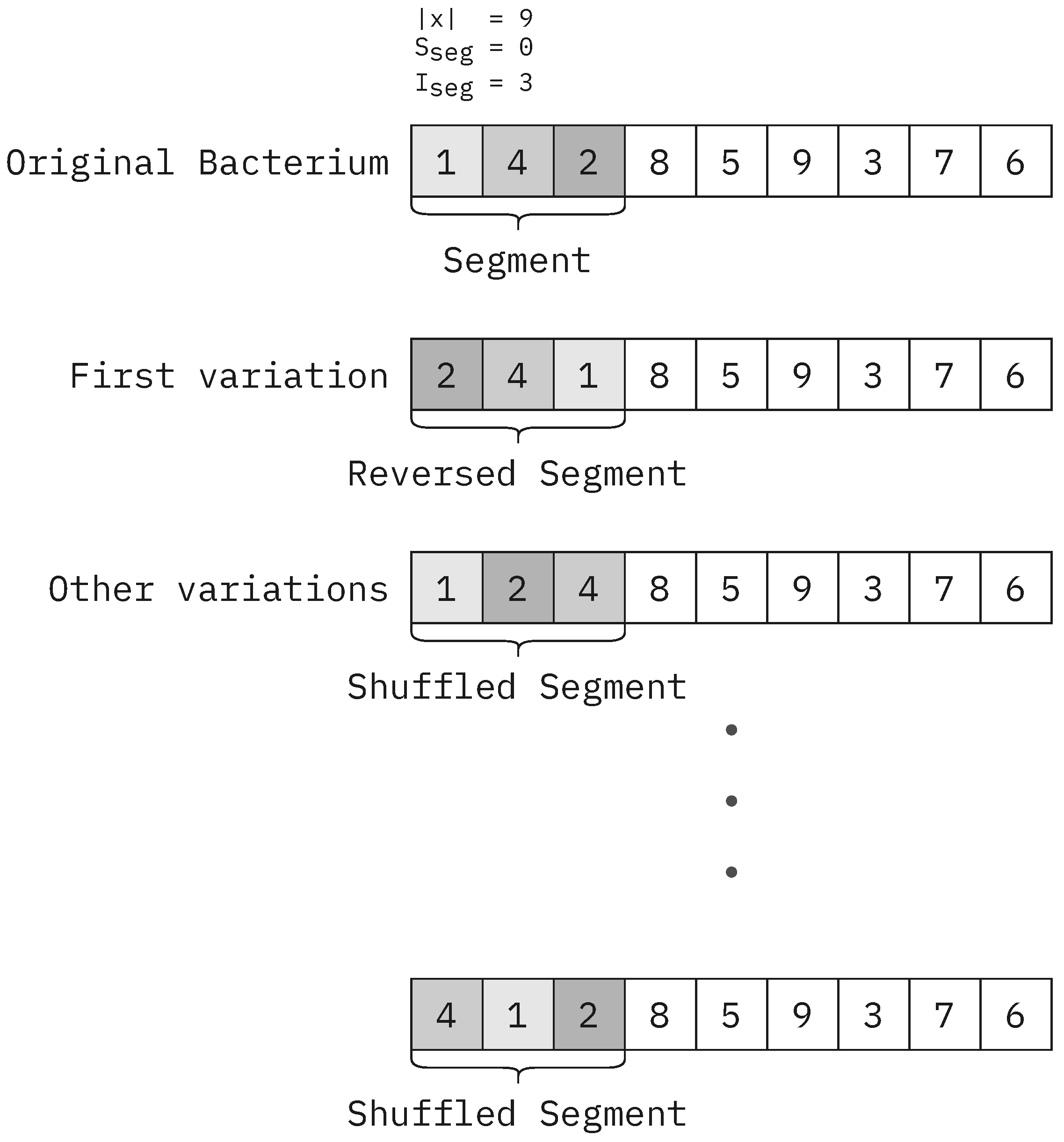
The $I_{seg}$ parameter is the length of the segment in the bacterial mutation operation. This value determines the size of the segment to be mutated to generate new mutant solutions. The larger the segment, the more varied the mutants will be. This parameter has a lesser impact on overall performance and runtime (See Figure 19). However, a value of four yielded the lowest standard deviation in runtime (See Figure 19c); therefore, it is the final parameter value chosen for our testing.

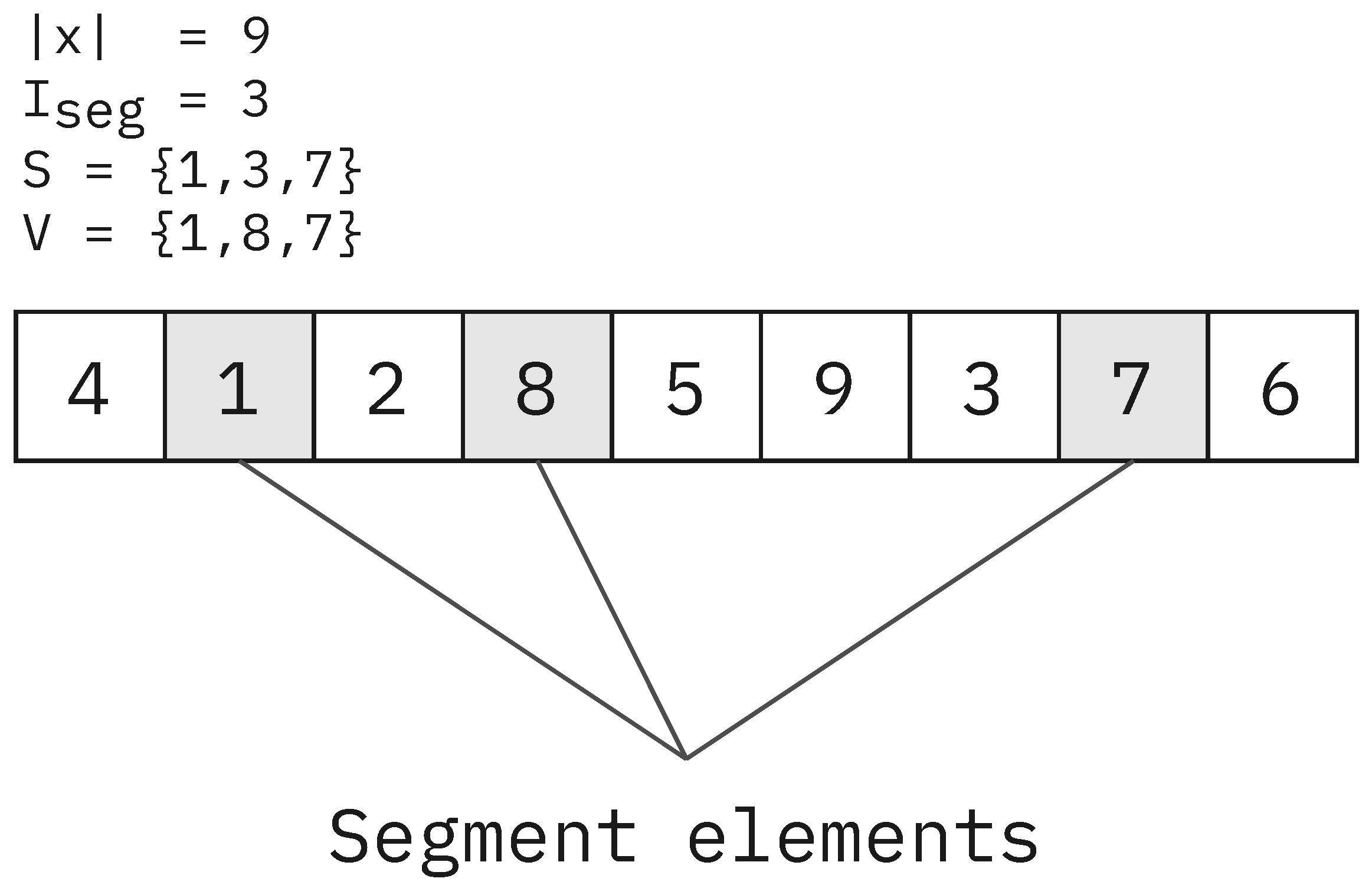
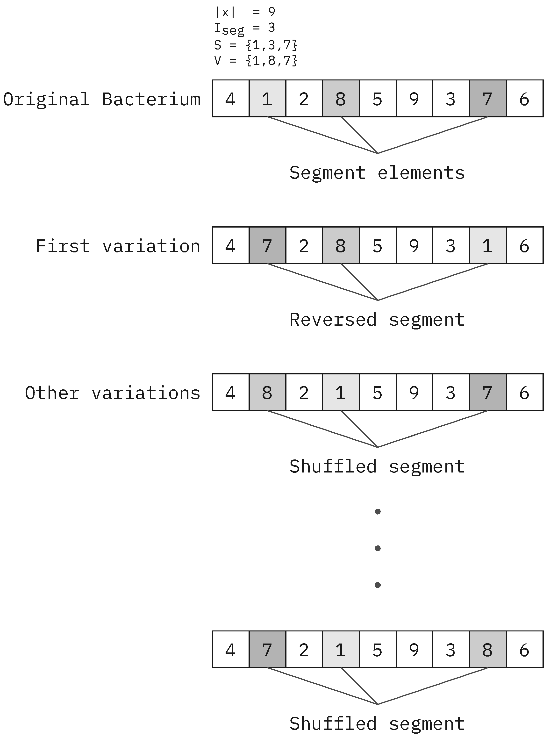
$I_{trans}$ is the length of the transferred segment in the gene transfer operation. A longer segment may increase the variance in generated solutions. However, in our testing, it had little impact on the quality of solutions (See Figure 20b,d) and runtimes (See Figure 20a,c). A value of four was chosen since it is a good middle-ground and it illustrates the workings of the operator well.

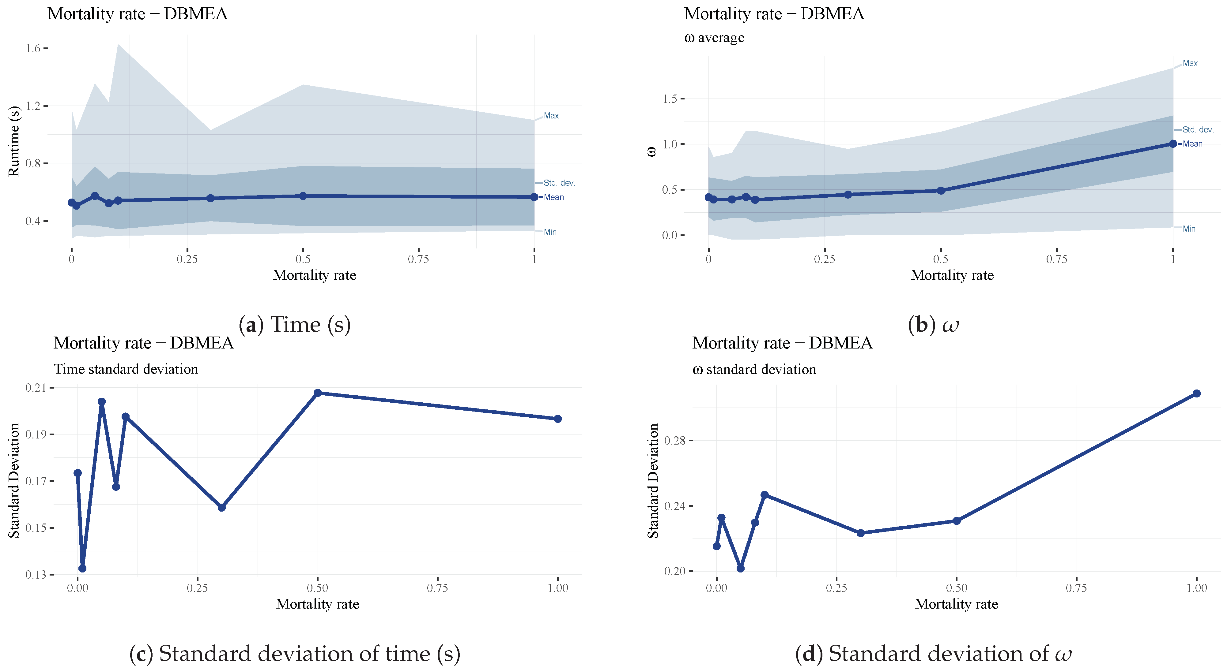
The mortality rate of $N_{mort}$ is the percentage of the population to be terminated at the end of each iteration (generation) and replaced with random solutions to increase diversity and escape local optima. A mortality rate of one creates a random population for each generation; a low mortality rate keeps more from the previous generation. Therefore, the mortality rate is an extension of elitism, where a portion of the population is kept instead of just one individual. It is evident that a high mortality rate (above 0.1) decreases the scheduling efficiency of the algorithm since the beneficial traits of previous generations are not carried forward (See Figure 21b,d). Too low of a value may increase the chance of the search being stuck in local optima. The mortality rate must be kept as high as possible without negating the traits of previous iterations. The parameter has almost no impact on the runtime of the algorithm (see Figure 21a,c). Considering the above, a mortality rate of 0.1 (10%) was chosen.

After our parameter analysis, a set of parameters were determined for the final testing on the entirety of the Taillard benchmark set. Table 1 contains all of the parameters chosen. These running parameters were used to obtain the results presented in Table A1, Table A2, Table A3 and

Table A4. Nine cases outperforming best known solutions.

Benchmark File	Task	Jobs	Machines	Makespan	Best Known
1tai20_5.txt	5	20	5	1235	1236
2tai20_10.txt	4	20	10	1377	1378
3tai20_20.txt	2	20	20	2099	2100
5tai50_10.txt	3	50	10	2863	2864
5tai50_10.txt	4	50	10	3063	3064
7tai100_5.txt	8	100	5	5098	5106
7tai100_5.txt	9	100	5	5448	5454
9tai100_20.txt	7	100	20	6342	6346
999tai200_20.txt	2	200	20	11,403	11,420

.

9. Conclusions

In this paper, we have described our proposed novel hybrid (extended “memetic” style) algorithm with a top-down approach and also provided details on the implementation. The results presented in this study demonstrate the efficiency of this new hybrid bacterial memetic algorithm in solving the flow-shop scheduling problem. As shown in Table A1 and Table A2, the algorithm has achieved a quality of solution comparable to the best-known results, with a difference of less than 1%. This comparison indicates that the algorithm can efficiently explore the solution space and produce high-quality solutions for many problems. Furthermore, our analysis of the algorithm’s performance on the Taillard benchmark set revealed that the hybrid bacterial memetic algorithm outperformed the best-known solutions for nine benchmark cases. The algorithm’s ability to solve complex scheduling problems has been made obvious.

To provide a comprehensive view of the algorithm’s performance, we have included Table A4, which summarizes the new best solutions obtained by the algorithm, along with their corresponding makespans. These results demonstrate the algorithm’s ability to find high-quality solutions that surpass the performance of all published methods.

The advantage of our proposed algorithm is its black-box approach to optimization, which implies that no assumption was made on the behaviour of the objective function. This approach allows for problem agnostic search as long as the solution requires a permutation as its solution. Therefore, we claim that our proposed algorithm can be used for the optimization of problems, which are even closer related to real-world tasks, like hybrid flow-shop scheduling with unrelated machines and machine eligibility [70] or extended job-shop scheduling [71]. One limitation of the algorithm is the number of times the objective function is called, increasing computation times drastically when more complex models are to be computed. Due to space and time constraints, these extended problems and respective solutions under increased complexity, like parallelization, have not been considered here. Overall, the hybrid bacterial memetic algorithm has shown great promise in solving the flow-shop scheduling problem, and it can potentially contribute to developing more efficient scheduling algorithms in the future. In our future work, we would like to investigate other use cases and refinements in performance, both in terms of scheduling ability and of compute time.

References

1. Onwubolu, G.C.; Babu, B. New Optimization Techniques in Engineering; Springer: Berlin/Heidelberg, Germany, 2013; Volume 141. [Google Scholar]
2. Tüu-Szabó, B.; Földesi, P.; Kóczy, L.T. An efficient evolutionary metaheuristic for the traveling repairman (minimum latency) problem. Int. J. Comput. Intell. Syst. 2020, 13, 781–793. [Google Scholar] [CrossRef]
3. Agárdi, A.; Nehéz, K.; Hornyák, O.; Kóczy, L.T. A Hybrid Discrete Bacterial Memetic Algorithm with Simulated Annealing for Optimization of the flow-shop scheduling problem. Symmetry 2021, 13, 1131. [Google Scholar] [CrossRef]
4. Balázs, K.; Botzheim, J.; Kóczy, L.T. Comparison of various evolutionary and memetic algorithms. In Integrated Uncertainty Management and Applications; Springer: Berlin/Heidelberg, Germany, 2010; pp. 431–442. [Google Scholar]
5. Nawa, N.E.; Furuhashi, T. Bacterial evolutionary algorithm for fuzzy system design. In SMC’98 Conference Proceedings, Proceedings of the 1998 IEEE International Conference on Systems, Man, and Cybernetics (Cat. No. 98CH36218), San Diego, CA, USA, 14 October 1998; IEEE: New York, NY, USA, 1998; Volume 3, pp. 2424–2429. [Google Scholar]
6. Moscato, P. On evolution, search, optimization, genetic algorithms and martial arts: Towards memetic algorithms. In Technical Report, Caltech Concurrent Computation Program Report 826; California Institute of Technology: Pasadena, CA, USA, 1989. [Google Scholar]
7. Wolpert, D.; Macready, W.G. No free lunch theorems for optimization. IEEE Trans. Evol. Comput. 1997, 1, 67–82. [Google Scholar] [CrossRef]
8. Kóczy, L.; Zorat, A. Fuzzy systems and approximation. Fuzzy Sets Syst. 1997, 85, 203–222. [Google Scholar] [CrossRef]
9. Kóczy, L.T. Symmetry or Asymmetry? Complex Problems and Solutions by Computational Intelligence and Soft Computing. Symmetry 2022, 14, 1839. [Google Scholar] [CrossRef]
10. Nawa, N.E.; Furuhashi, T. Fuzzy system parameters discovery by bacterial evolutionary algorithm. IEEE Trans. Fuzzy Syst. 1999, 7, 608–616. [Google Scholar] [CrossRef]
11. Botzheim, J.; Cabrita, C.; Kóczy, L.T.; Ruano, A. Fuzzy rule extraction by bacterial memetic algorithms. Int. J. Intell. Syst. 2009, 24, 312–339. [Google Scholar] [CrossRef]
12. Das, S.; Chowdhury, A.; Abraham, A. A bacterial evolutionary algorithm for automatic data clustering. In Proceedings of the 2009 IEEE Congress on Evolutionary Computation, Trondheim, Norway, 18–21 May 2009; pp. 2403–2410. [Google Scholar]
13. Hoos, H.H.; Stützle, T. Stochastic Local Search: Foundations and Applications; Elsevier: Amsterdam, The Netherlands, 2004. [Google Scholar]
14. Moré, J.J. The Levenberg-Marquardt algorithm: Implementation and theory. In Numerical Analysis; Springer: Berlin/Heidelberg, Germany, 1978; pp. 105–116. [Google Scholar]
15. Gong, G.; Deng, Q.; Chiong, R.; Gong, X.; Huang, H. An effective memetic algorithm for multi-objective job-shop scheduling. Knowl.-Based Syst. 2019, 182, 104840. [Google Scholar] [CrossRef]
16. Yamada, T.; Nakano, R. A fusion of crossover and local search. In Proceedings of the IEEE International Conference on Industrial Technology (ICIT’96), Shanghai, China, 2–6 December 1996; pp. 426–430. [Google Scholar]
17. Muyldermans, L.; Beullens, P.; Cattrysse, D.; Van Oudheusden, D. Exploring variants of 2-opt and 3-opt for the general routing problem. Oper. Res. 2005, 53, 982–995. [Google Scholar] [CrossRef]
18. Balazs, K.; Koczy, L.T. Hierarchical-interpolative fuzzy system construction by genetic and bacterial memetic programming approaches. Int. J. Uncertain. Fuzziness Knowl.-Based Syst. 2012, 20, 105–131. [Google Scholar] [CrossRef]
19. Pinedo, M. Scheduling: Theory, Algorithms, and Systems, 5th ed.; Springer: Cham, Switzerland, 2016. [Google Scholar]
20. Johnson, S.M. Optimal two-and three-stage production schedules with setup times included. Nav. Res. Logist. Q. 1954, 1, 61–68. [Google Scholar] [CrossRef]
21. Garey, M.R.; Johnson, D.S.; Sethi, R. The complexity of flowshop and jobshop scheduling. Math. Oper. Res. 1976, 1, 117–129. [Google Scholar] [CrossRef]
22. Nawaz, M.; Enscore, E.E., Jr.; Ham, I. A heuristic algorithm for the m-machine, n-job flow-shop sequencing problem. Omega 1983, 11, 91–95. [Google Scholar] [CrossRef]
23. Taillard, E. Benchmarks for basic scheduling problems. Eur. J. Oper. Res. 1993, 64, 278–285. [Google Scholar] [CrossRef]
24. Van Laarhoven, P.J.; Aarts, E.H. simulated annealing. In Simulated Annealing: Theory and Applications; Springer: Berlin/Heidelberg, Germany, 1987; pp. 7–15. [Google Scholar]
25. Dai, M.; Tang, D.; Giret, A.; Salido, M.A.; Li, W.D. Energy-efficient scheduling for a flexible flow shop using an improved genetic-simulated annealing algorithm. Robot. Comput.-Integr. Manuf. 2013, 29, 418–429. [Google Scholar] [CrossRef]
26. Jouhari, H.; Lei, D.; A. A. Al-qaness, M.; Abd Elaziz, M.; Ewees, A.A.; Farouk, O. Sine-Cosine Algorithm to Enhance simulated annealing for Unrelated Parallel Machine Scheduling with Setup Times. Mathematics 2019, 7, 1120. [Google Scholar] [CrossRef]
27. Alnowibet, K.A.; Mahdi, S.; El-Alem, M.; Abdelawwad, M.; Mohamed, A.W. Guided Hybrid Modified simulated annealing Algorithm for Solving Constrained Global Optimization Problems. Mathematics 2022, 10, 1312. [Google Scholar] [CrossRef]
28. Suanpang, P.; Jamjuntr, P.; Jermsittiparsert, K.; Kaewyong, P. Tourism Service Scheduling in Smart City Based on Hybrid Genetic Algorithm simulated annealing Algorithm. Sustainability 2022, 14, 6293. [Google Scholar] [CrossRef]
29. Redi, A.A.N.P.; Jewpanya, P.; Kurniawan, A.C.; Persada, S.F.; Nadlifatin, R.; Dewi, O.A.C. A simulated annealing Algorithm for Solving Two-Echelon Vehicle Routing Problem with Locker Facilities. Algorithms 2020, 13, 218. [Google Scholar] [CrossRef]
30. Rahimi, A.; Hejazi, S.M.; Zandieh, M.; Mirmozaffari, M. A Novel Hybrid simulated annealing for No-Wait Open-Shop Surgical Case Scheduling Problems. Appl. Syst. Innov. 2023, 6, 15. [Google Scholar] [CrossRef]
31. Bean, J.C. Genetic algorithms and random keys for sequencing and optimization. ORSA J. Comput. 1994, 6, 154–160. [Google Scholar] [CrossRef]
32. Hansen, P.; Mladenović, N. Variable neighborhood search: Principles and applications. Eur. J. Oper. Res. 2001, 130, 449–467. [Google Scholar] [CrossRef]
33. Tasgetiren, M.F.; Liang, Y.C.; Sevkli, M.; Gencyilmaz, G. A particle swarm optimization algorithm for makespan and total flowtime minimization in the permutation flowshop sequencing problem. Eur. J. Oper. Res. 2007, 177, 1930–1947. [Google Scholar] [CrossRef]
34. Liao, C.J.; Tseng, C.T.; Luarn, P. A discrete version of particle swarm optimization for flowshop scheduling problems. Comput. Oper. Res. 2007, 34, 3099–3111. [Google Scholar] [CrossRef]
35. Jarboui, B.; Ibrahim, S.; Siarry, P.; Rebai, A. A combinatorial particle swarm optimisation for solving permutation flowshop problems. Comput. Ind. Eng. 2008, 54, 526–538. [Google Scholar] [CrossRef]
36. Marchetti-Spaccamela, A.; Crama, Y.; Goossens, D.; Leus, R.; Schyns, M.; Spieksma, F. Proceedings of the 12th Workshop on Models and Algorithms for Planning and Scheduling Problems. 2015. Available online: https://feb.kuleuven.be/mapsp2015/Proceedings%20MAPSP%202015.pdf (accessed on 23 August 2023).
37. Glover, F.; Laguna, M.; Marti, R. Scatter search and path relinking: Advances and applications. In Handbook of Metaheuristics; Springer: Berlin/Heidelberg, Germany, 2003; pp. 1–35. [Google Scholar]
38. Resende, M.G.; Ribeiro, C.C.; Glover, F.; Martí, R. Scatter search and path-relinking: Fundamentals, advances, and applications. In Handbook of Metaheuristics; Springer: Berlin/Heidelberg, Germany, 2010; pp. 87–107. [Google Scholar]
39. Marinakis, Y.; Marinaki, M. Particle swarm optimization with expanding neighborhood topology for the permutation flowshop scheduling problem. Soft Comput. 2013, 17, 1159–1173. [Google Scholar] [CrossRef]
40. Ying, K.C.; Liao, C.J. An ant colony system for permutation flow-shop sequencing. Comput. Oper. Res. 2004, 31, 791–801. [Google Scholar] [CrossRef]
41. Colorni, A.; Dorigo, M.; Maniezzo, V. Distributed optimization by ant colonies. In Proceedings of the First European Conference on Artificial Life, Paris, France, 11–13 December 1991; Volume 142, pp. 134–142. [Google Scholar]
42. Colorni, A.; Dorigo, M.; Maniezzo, V. A Genetic Algorithm to Solve the Timetable Problem; Politecnico di Milano: Milan, Italy, 1992. [Google Scholar]
43. Hayat, I.; Tariq, A.; Shahzad, W.; Masud, M.; Ahmed, S.; Ali, M.U.; Zafar, A. Hybridization of Particle Swarm Optimization with Variable Neighborhood Search and simulated annealing for Improved Handling of the Permutation Flow-Shop Scheduling Problem. Systems 2023, 11, 221. [Google Scholar] [CrossRef]
44. Chen, S.H.; Chang, P.C.; Cheng, T.; Zhang, Q. A self-guided genetic algorithm for permutation flowshop scheduling problems. Comput. Oper. Res. 2012, 39, 1450–1457. [Google Scholar] [CrossRef]
45. Baraglia, R.; Hidalgo, J.I.; Perego, R. A hybrid heuristic for the traveling salesman problem. IEEE Trans. Evol. Comput. 2001, 5, 613–622. [Google Scholar] [CrossRef]
46. Harik, G.R.; Lobo, F.G.; Goldberg, D.E. The compact genetic algorithm. IEEE Trans. Evol. Comput. 1999, 3, 287–297. [Google Scholar] [CrossRef]
47. Mühlenbein, H.; Paaß, G. From recombination of genes to the estimation of distributions I. Binary parameters. In International Conference on Parallel Problem Solving from Nature; Springer: Berlin/Heidelberg, Germany, 1996; pp. 178–187. [Google Scholar]
48. Pelikan, M.; Goldberg, D.E.; Lobo, F.G. A survey of optimization by building and using probabilistic models. Comput. Optim. Appl. 2002, 21, 5–20. [Google Scholar] [CrossRef]
49. Storn, R.; Price, K. Differential evolution–a simple and efficient heuristic for global optimization over continuous spaces. J. Glob. Optim. 1997, 11, 341–359. [Google Scholar] [CrossRef]
50. Tasgetiren, M.F.; Pan, Q.K.; Suganthan, P.N.; Liang, Y.C. A discrete differential evolution algorithm for the no-wait flowshop scheduling problem with total flowtime criterion. In Proceedings of the 2007 IEEE Symposium on Computational Intelligence in Scheduling, Honolulu, HI, USA, 1–5 April 2007; pp. 251–258. [Google Scholar]
51. Pan, Q.K.; Tasgetiren, M.F.; Liang, Y.C. A discrete differential evolution algorithm for the permutation flowshop scheduling problem. Comput. Ind. Eng. 2008, 55, 795–816. [Google Scholar] [CrossRef]
52. Zobolas, G.; Tarantilis, C.D.; Ioannou, G. Minimizing makespan in permutation flow-shop scheduling problems using a hybrid metaheuristic algorithm. Comput. Oper. Res. 2009, 36, 1249–1267. [Google Scholar] [CrossRef]
53. Mehrabian, A.R.; Lucas, C. A novel numerical optimization algorithm inspired from weed colonization. Ecol. Inform. 2006, 1, 355–366. [Google Scholar] [CrossRef]
54. Zhou, Y.; Chen, H.; Zhou, G. Invasive weed optimization algorithm for optimization no-idle flow shop scheduling problem. Neurocomputing 2014, 137, 285–292. [Google Scholar] [CrossRef]
55. Wei, H.; Li, S.; Jiang, H.; Hu, J.; Hu, J. Hybrid genetic simulated annealing algorithm for improved flow shop scheduling with makespan criterion. Appl. Sci. 2018, 8, 2621. [Google Scholar] [CrossRef]
56. Tseng, L.Y.; Lin, Y.T. A hybrid genetic algorithm for no-wait flowshop scheduling problem. Int. J. Prod. Econ. 2010, 128, 144–152. [Google Scholar] [CrossRef]
57. Qu, C.; Fu, Y.; Yi, Z.; Tan, J. Solutions to no-wait flow-shop scheduling problem using the flower pollination algorithm based on the hormone modulation mechanism. Complexity 2018, 2018, 1973604. [Google Scholar] [CrossRef]
58. Alawad, N.A.; Abed-alguni, B.H. Discrete Jaya with refraction learning and three mutation methods for the permutation flow-shop scheduling problem. J. Supercomput. 2022, 78, 3517–3538. [Google Scholar] [CrossRef]
59. Gao, K.; Yang, F.; Zhou, M.; Pan, Q.; Suganthan, P.N. Flexible job-shop rescheduling for new job insertion by using discrete Jaya algorithm. IEEE Trans. Cybern. 2018, 49, 1944–1955. [Google Scholar] [CrossRef]
60. Fathollahi-Fard, A.M.; Woodward, L.; Akhrif, O. Sustainable distributed permutation flow-shop scheduling model based on a triple bottom line concept. J. Ind. Inf. Integr. 2021, 24, 100233. [Google Scholar] [CrossRef]
61. Baroud, M.M.; Eghtesad, A.; Mahdi, M.A.A.; Nouri, M.B.B.; Khordehbinan, M.W.W.; Lee, S. A New Method for Solving the flow-shop scheduling problem on Symmetric Networks Using a Hybrid Nature-Inspired Algorithm. Symmetry 2023, 15, 1409. [Google Scholar] [CrossRef]
62. Liang, Z.; Zhong, P.; Liu, M.; Zhang, C.; Zhang, Z. A computational efficient optimization of flow shop scheduling problems. Sci. Rep. 2022, 12, 845. [Google Scholar] [CrossRef] [PubMed]
63. Alireza, A.; Javid, G.N.; Hamed, N. Flexible flow shop scheduling with forward and reverse flow under uncertainty using the red deer algorithm. J. Ind. Eng. Manag. Stud. 2023, 10, 16–33. [Google Scholar]
64. Kóczy, L.T.; Földesi, P.; Tüű-Szabó, B. An effective discrete bacterial memetic evolutionary algorithm for the traveling salesman problem. Int. J. Intell. Syst. 2017, 32, 862–876. [Google Scholar] [CrossRef]
65. Agárdi, A.; Nehéz, K. Parallel machine scheduling with Monte Carlo Tree Search. Acta Polytech. 2021, 61, 307–312. [Google Scholar] [CrossRef]
66. Wu, T.Y.; Wu, I.C.; Liang, C.C. Multi-objective flexible job shop scheduling problem based on monte-carlo tree search. In Proceedings of the 2013 Conference on Technologies and Applications of Artificial Intelligence, Taipei, Taiwan, 6–8 December 2013; pp. 73–78. [Google Scholar]
67. Kocsis, L.; Szepesvári, C. Bandit based monte-carlo planning. In European Conference on Machine Learning, Proceedings of the ECML 2006, Berlin, Germany, 18–22 September 2006; Proceedings 17; Springer: Berlin/Heidelberg, Germany, 2006; pp. 282–293. [Google Scholar]
68. Kirkpatrick, S.; Gelatt, C.D.; Vecchi, M.P. Optimization by simulated annealing. Science 1983, 220, 671–680. [Google Scholar] [CrossRef]
69. Miliczki, J.; Fazekas, L. Comparison of Cooling Strategies in simulated annealing Algorithms for Flow-shop Scheduling. Prod. Syst. Inf. Eng. 2022, 10, 129–136. [Google Scholar] [CrossRef]
70. Yu, C.; Semeraro, Q.; Matta, A. A genetic algorithm for the hybrid flow shop scheduling with unrelated machines and machine eligibility. Comput. Oper. Res. 2018, 100, 211–229. [Google Scholar] [CrossRef]
71. Shi, L.; Ólafsson, S.; Shi, L.; Ólafsson, S. Extended Job Shop Scheduling. Nested Partitions Method, Theory and Applications; Springer: Berlin/Heidelberg, Germany, 2009; pp. 207–225. [Google Scholar]
72. Marinakis, Y.; Marinaki, M. Hybrid Adaptive Particle Swarm Optimization Algorithm for the Permutation Flowshop Scheduling Problem. In Proceedings of the 13th Workshop on Models and Algorithms for Planning and Scheduling Problems, Abbey, Germany, 12–16 June 2017; p. 189. [Google Scholar]
Figure 1. Example of the first job not waiting.
Algorithms 16 00406 g001
Figure 2. Example of jobs on the first machine.
Algorithms 16 00406 g002
Figure 3. Contingency of start times.
Algorithms 16 00406 g003
Figure 4. Example for obtaining C m a x .
Algorithms 16 00406 g004
Figure 5. Cohesive segments chosen in Algorithm 2. (a) Chosen segment, when S s e g = I s e g · i = 0 ; (b) chosen segment, when S s e g = I s e g · i = 3 ; (c) chosen segment, when S s e g = I s e g · i = 6 ; and (d) all the segments chosen throughout the algorithm.
Algorithms 16 00406 g005
Figure 6. Cohesive segment process in Algorithm 3.
Algorithms 16 00406 g006
Figure 7. Example for a segment chosen in loose segment mutation (Algorithm 4).
Algorithms 16 00406 g007
Figure 8. Loose segment mutation in Algorithm 4.
Algorithms 16 00406 g008
Figure 9. Gene transfer mutation.
Algorithms 16 00406 g009
Figure 10. Monte Carlo tree search.
Algorithms 16 00406 g010
Figure 11. Analysis of the maximum iteration count (SA) parameter.
Algorithms 16 00406 g011
Figure 12. Analysis of the starting temperature (SA) parameter.
Algorithms 16 00406 g012
Figure 13. Analysis of the α parameter.
Algorithms 16 00406 g013
Figure 14. Analysis of the iteration count (MCTS) parameter.
Algorithms 16 00406 g014
Figure 15. Analysis of the N i n d parameter.
Algorithms 16 00406 g015
Figure 16. Analysis of the DBMEA maximum iteration count.
Algorithms 16 00406 g016
Figure 17. Analysis of the N c l o n e s parameter.
Algorithms 16 00406 g017
Figure 18. Analysis of the N i n f parameter.
Algorithms 16 00406 g018
Figure 19. Analysis of the I s e g parameter.
Algorithms 16 00406 g019
Figure 20. Analysis of the I t r a n s parameter.
Algorithms 16 00406 g020
Figure 21. Analysis of the N m o r t parameter.
Algorithms 16 00406 g021