
A Heterogeneity-Aware Car-Following Model: Based on the XGBoost Method

Abstract
1. Introduction
- Current car-following models are too limited in consideration of human-likeness. In theory-driven models, only a few factors are typically included due to the increased complexity that arises from incorporating additional parameters. Furthermore, quantifying certain factors into physically meaningful parameters can be challenging. In data-driven models, the current focus of research primarily revolves around using deep learning models to directly emulate human behavior, often overlooking the consideration of heterogeneity factors. As mentioned before, research on behavioral heterogeneity factors has been extensively analyzed to determine whether they have an impact on car-following behavior. However, these factors are not fully considered in the construction of car-following models in the field of autonomous driving.
- 2.
- Current car-following models mainly use theory-driven models and deep learning models; the choice of models can be expanded. Incorporating heterogeneity factors into theory-driven models often leads to more parameters, making model calibration challenging. Deep learning models have good performance, but they have complex structures, resource-intensive requirements, and low interpretability. Ensemble learning models provide a promising avenue for further exploration. It can imitate human behavior through machine learning, and it can also embed other heterogeneous factors artificially. Crucially, the ensemble learning model has strong learning ability and is lightweight, which are two of the key factors applied in actual autonomous driving systems.
- (1)
- Incorporating the heterogeneity factors of car-following behavior into the car-following model to achieve more human-like car-following performance.
- (2)
- Apply decision tree-based ensemble learning algorithms for the data-driven car-following model, which can partially overcome the issues of deep learning models’ lack of interpretability and high latency.
- (3)
- This paper quantifies the impact of heterogeneity factors on car-following behavior. That helps researchers better understand the effect of heterogeneity in car-following modeling.
2. Materials and Methodology
2.1. Data and Variables
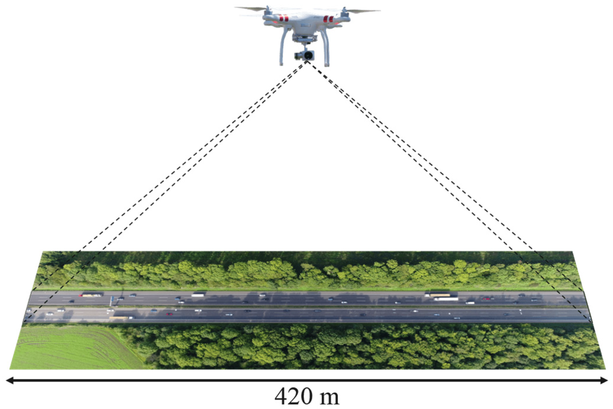
2.1.1. Data Description
2.1.2. Data Pre-Processing
- Exclude distance headways larger than 150 m to guarantee the influence of the heading vehicle.
- Exclude the situation of the dangerous car following the scenario where the relative distance is less than 50 m and the relative speed is greater than 3 m/s.
2.1.3. Input and Output Variables
2.2. Methodology
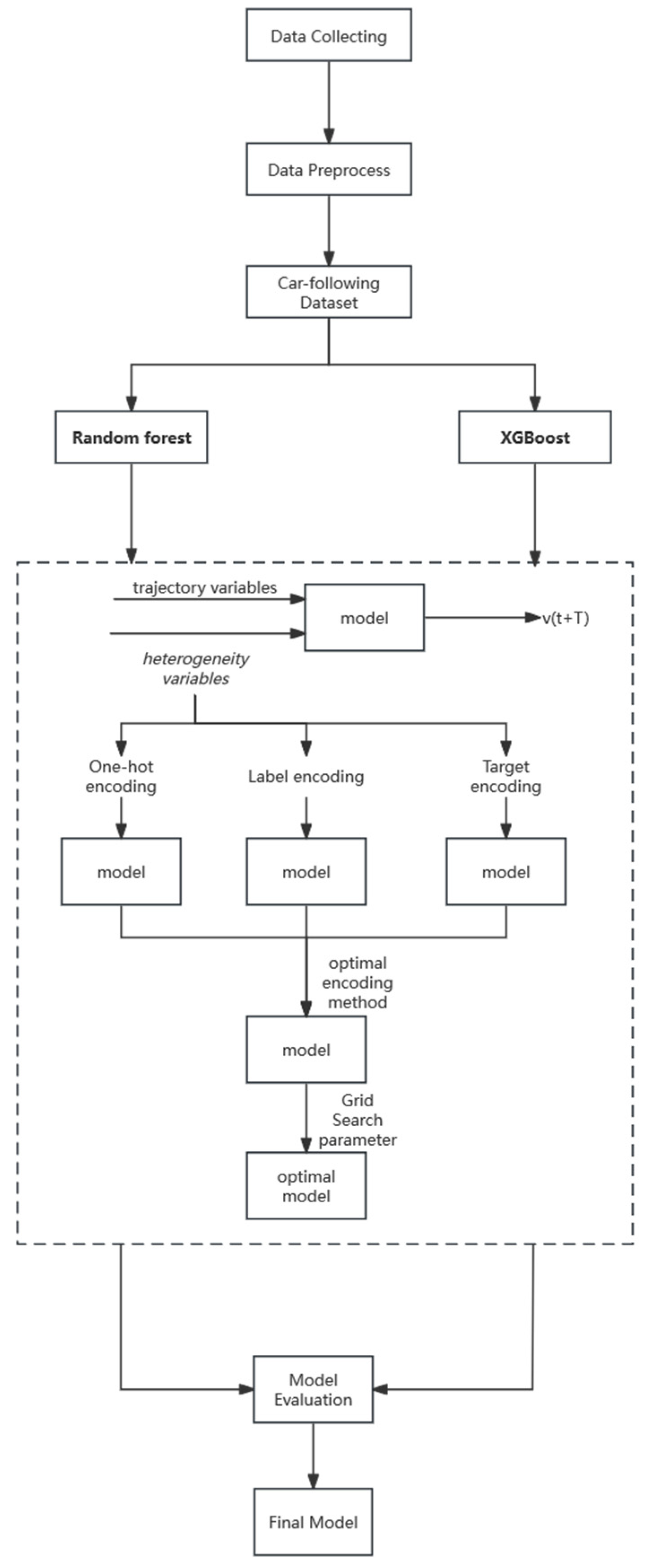
2.2.1. The Design of the Experimental Process
2.2.2. Ensemble Learning
2.2.3. Random Forest Method
2.2.4. XGBoost Method
2.2.5. Encoding Methods
2.2.6. Evaluation Metrics
3. Application of the Proposed Methodology
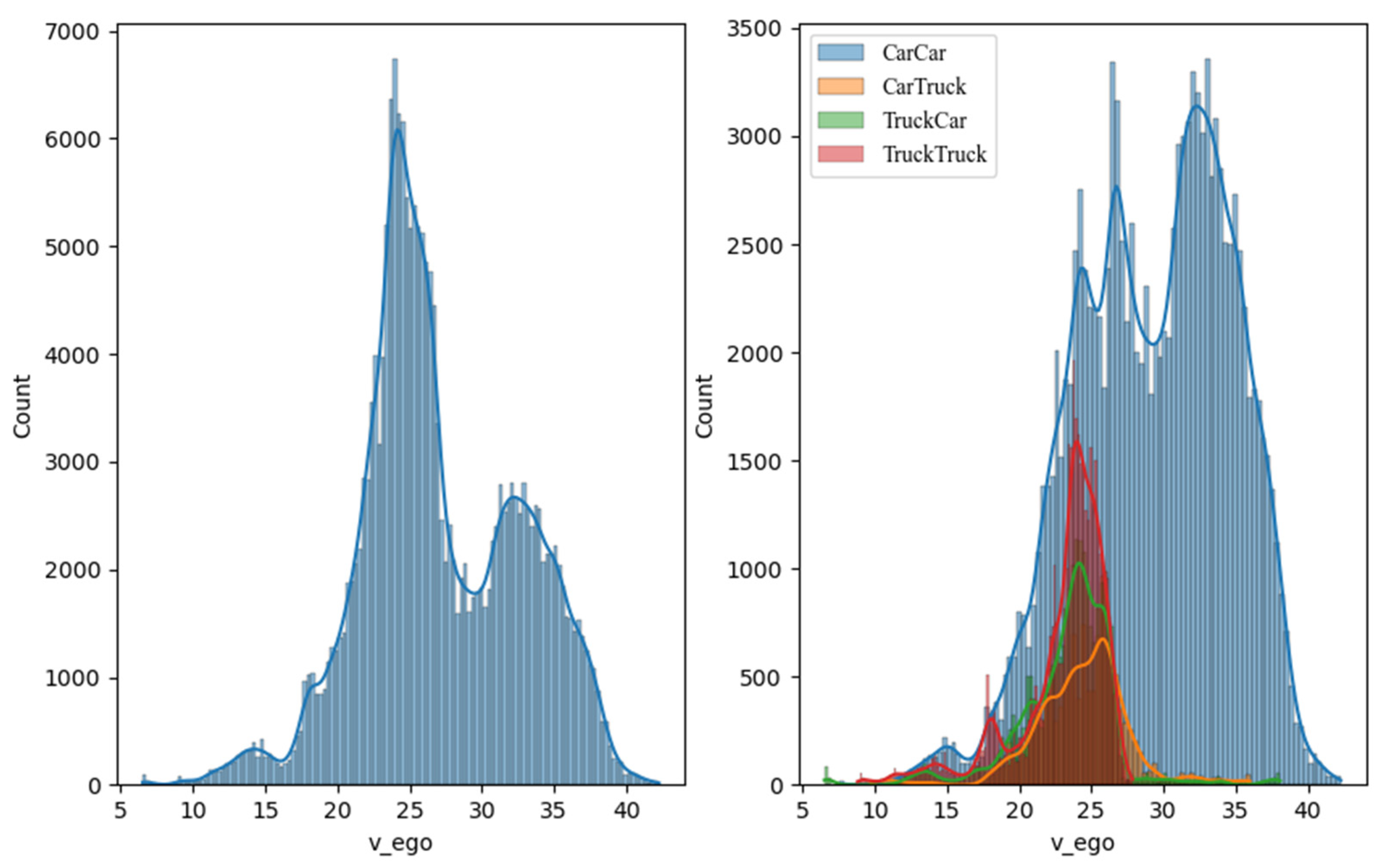
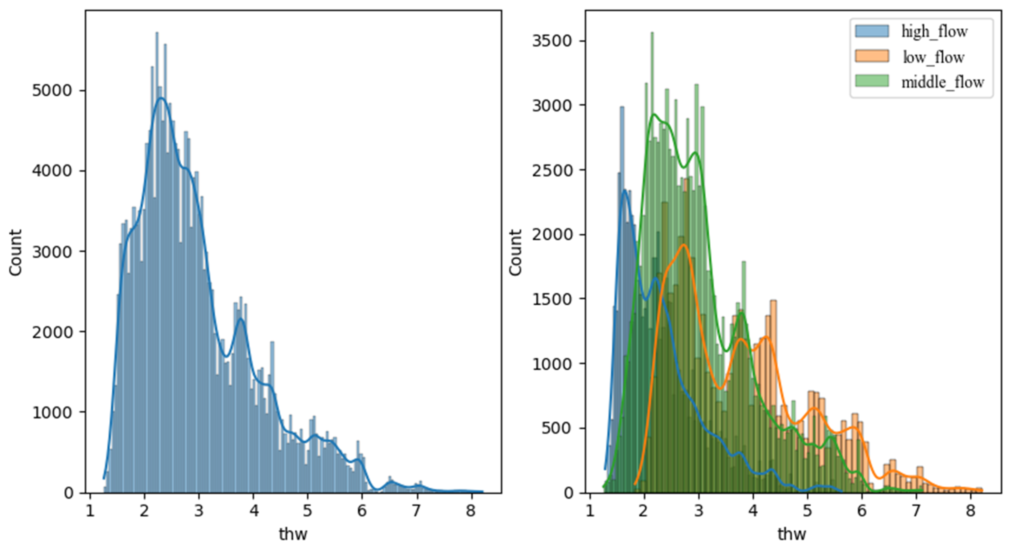
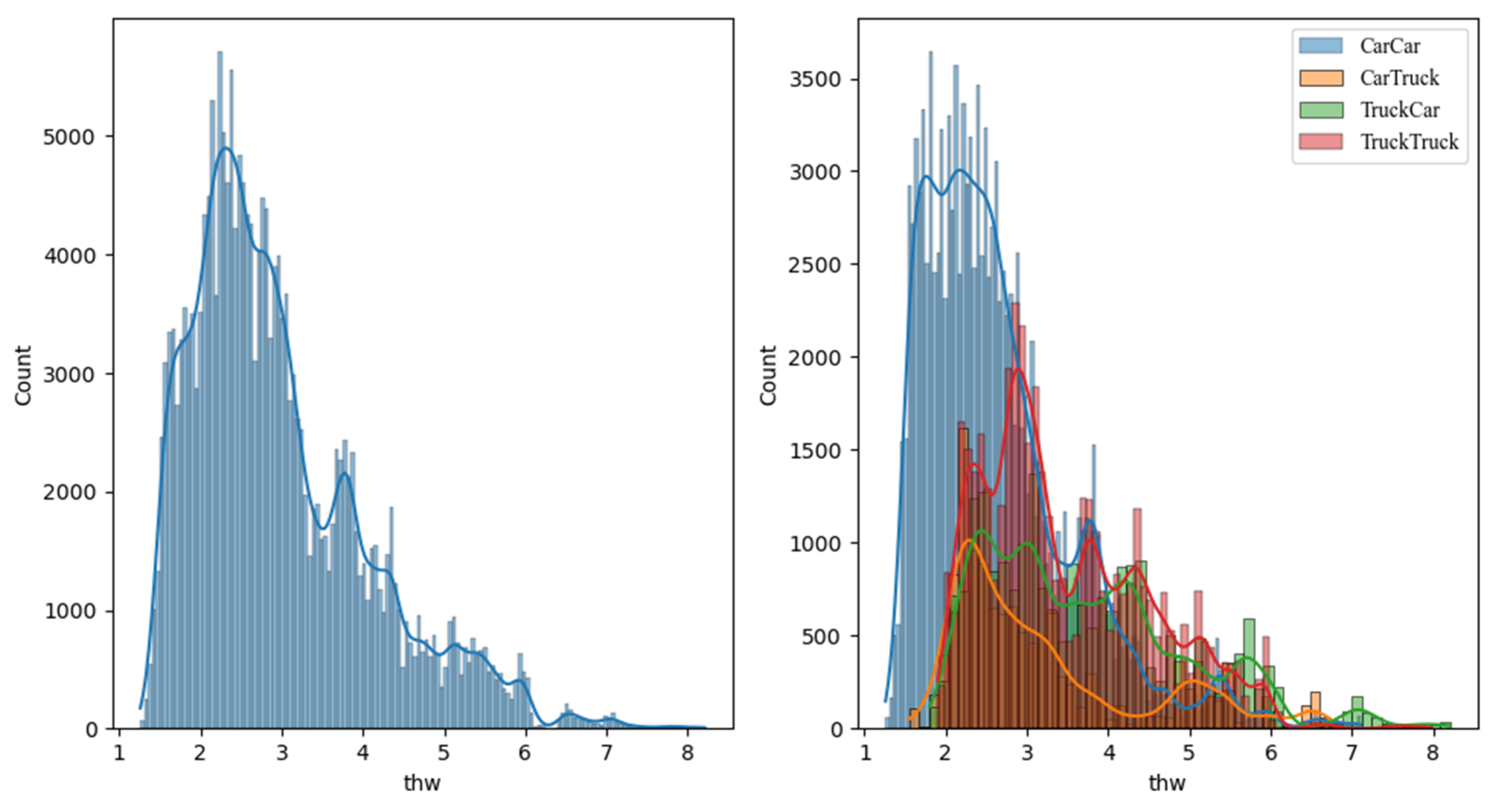
3.1. Heterogeneity in Car-Following Behavior Analysis
3.2. Suitable Encoder for Heterogeneity Variables
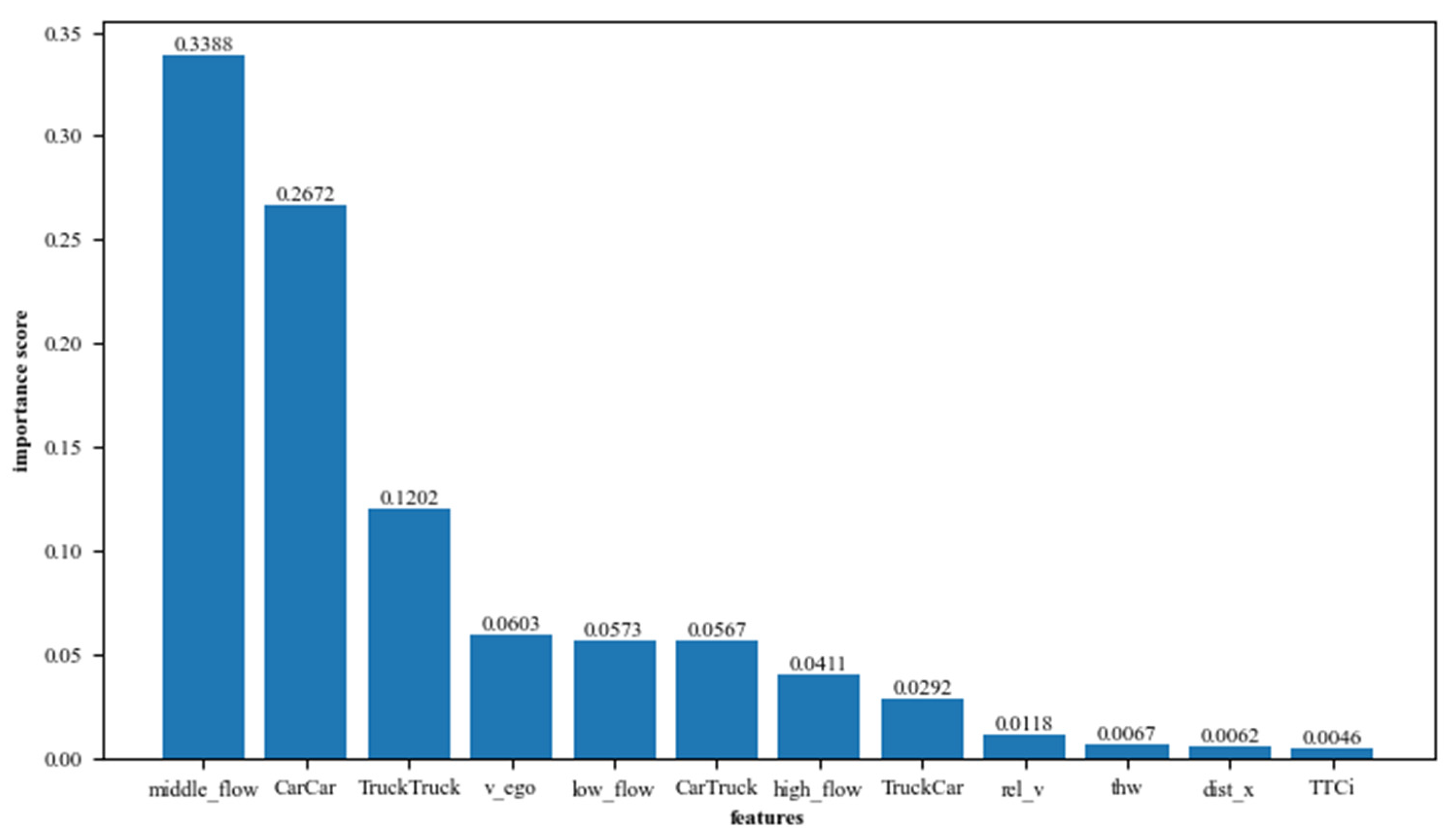
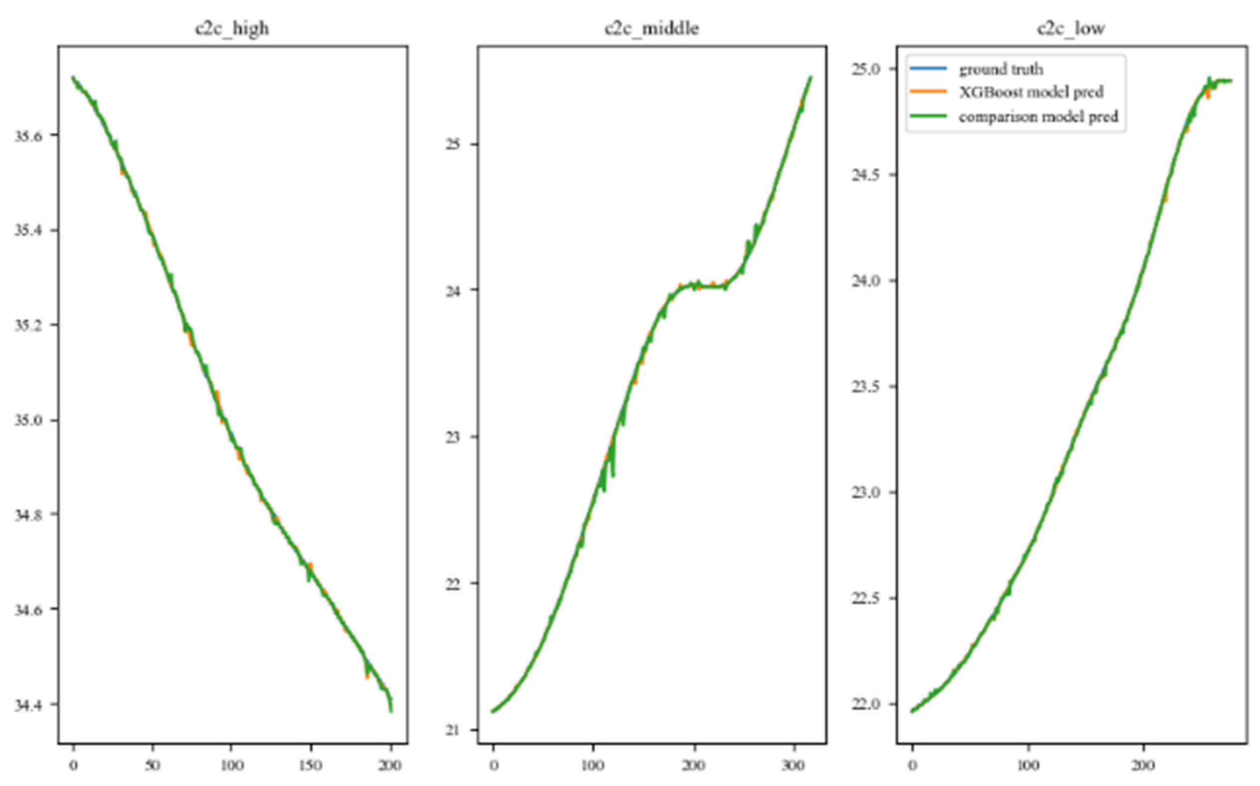
3.3. The Model Experiments Result
3.4. The Ablation Experiments Result
4. Conclusions and Discussion
Author Contributions
Funding
Data Availability Statement
Conflicts of Interest
References
- Yang, L.; Zhang, C.; Qiu, X.; Li, S.; Wang, H. Research progress on car-following models. J. Traffic Transp. Eng. 2019, 19, 125–138. [Google Scholar] [CrossRef]
- An, S.-H.; Lee, B.-H.; Shin, D.-R. A Survey of Intelligent Transportation Systems. In Proceedings of the 2011 3rd International Conference on Computational Intelligence, Communication Systems and Networks, Bali, Indonesia, 26–28 July 2011; pp. 332–337. [Google Scholar] [CrossRef]
- Hoogendoorn, S.P.; Bovy, P.H.L. State-of-the-art of vehicular traffic flow modelling. Proc. Inst. Mech. Eng. Part I J. Syst. Control Eng. 2001, 215, 283–303. [Google Scholar] [CrossRef]
- Pipes, L.A. An Operational Analysis of Traffic Dynamics. J. Appl. Phys. 1953, 24, 274–281. [Google Scholar] [CrossRef]
- Chandler, R.E.; Herman, R.; Montroll, E.W. Traffic Dynamics: Studies in Car Following. Oper. Res. 1958, 6, 165–184. [Google Scholar] [CrossRef]
- Treiber, M.; Hennecke, A.; Helbing, D. Congested traffic states in empirical observations and microscopic simulations. Phys. Rev. E 2000, 62, 1805–1824. [Google Scholar] [CrossRef] [PubMed]
- Newell, G.F. Nonlinear Effects in the Dynamics of Car Following. Oper. Res. 1961, 9, 209–229. [Google Scholar] [CrossRef]
- Saifuzzaman, M.; Zheng, Z.; Haque, M.; Washington, S. Revisiting the Task–Capability Interface model for incorporating human factors into car-following models. Transp. Res. Part B Methodol. 2015, 82, 1–19. [Google Scholar] [CrossRef]
- Treiber, M.; Kesting, A. The Intelligent Driver Model with Stochasticity—New Insights into Traffic Flow Oscillations. Transp. Res. Procedia 2017, 23, 174–187. [Google Scholar] [CrossRef]
- Kehtarnavaz, N.; Groswold, N.; Miller, K.; Lascoe, P. A transportable neural-network approach to autonomous vehicle following. IEEE Trans. Veh. Technol. 1998, 47, 694–702. [Google Scholar] [CrossRef]
- Dabiri, S.; Abbas, M. Evaluation of the Gradient Boosting of Regression Trees Method on Estimating Car-Following Behavior. Transp. Res. Rec. 2018, 2672, 136–146. [Google Scholar] [CrossRef]
- Ma, X. A Neural-Fuzzy Framework for Modeling Car-following Behavior. In Proceedings of the 2006 IEEE International Conference on Systems, Man and Cybernetics, Taipei, Taiwan, 8–11 October 2006; Volume 2, pp. 1178–1183. [Google Scholar] [CrossRef]
- Khodayari, A.; Ghaffari, A.; Kazemi, R.; Braunstingl, R. A Modified Car-Following Model Based on a Neural Network Model of the Human Driver Effects. IEEE Trans. Syst. Man Cybern. A 2012, 42, 1440–1449. [Google Scholar] [CrossRef]
- Zhang, W.; Zhao, J.; Quan, P.; Wang, J.; Meng, X.; Li, Q. Prediction of influent wastewater quality based on wavelet transform and residual LSTM. Appl. Soft Comput. 2023, 148, 110858. [Google Scholar] [CrossRef]
- Wang, X.; Jiang, R.; Li, L.; Lin, Y.; Zheng, X.; Wang, F.-Y. Capturing Car-Following Behaviors by Deep Learning. IEEE Trans. Intell. Transp. Syst. 2018, 19, 910–920. [Google Scholar] [CrossRef]
- Fan, P.; Guo, J.; Zhao, H.; Wijnands, J.S.; Wang, Y. Car-Following Modeling Incorporating Driving Memory Based on Autoencoder and Long Short-Term Memory Neural Networks. Sustainability 2019, 11, 6755. [Google Scholar] [CrossRef]
- Ossen, S.; Hoogendoorn, S.P. Multi-anticipation and heterogeneity in car-following empirics and a first exploration of their implications. In Proceedings of the 2006 IEEE Intelligent Transportation Systems Conference, Toronto, ON, Canada, 17–20 September 2006; pp. 1615–1620. [Google Scholar] [CrossRef]
- Ossen, S.; Hoogendoorn, S.P.; Gorte, B.G.H. Interdriver Differences in Car-Following. Transp. Res. Rec. 2006, 1965, 121–129. [Google Scholar] [CrossRef]
- Ossen, S.; Hoogendoorn, S.P. Heterogeneity in car-following behavior: Theory and empirics. Transp. Res. Part C Emerg. Technol. 2011, 19, 182–195. [Google Scholar] [CrossRef]
- Zheng, L.; Zhu, C.; He, Z.; He, T.; Liu, S. Empirical validation of vehicle type-dependent car-following heterogeneity from micro- and macro-viewpoints. Transp. B Transp. Dyn. 2019, 7, 765–787. [Google Scholar] [CrossRef]
- Zhang, Y.; Ni, P.; Li, M.; Liu, H.; Yin, B. A New Car-Following Model considering Driving Characteristics and Preceding Vehicle’s Acceleration. J. Adv. Transp. 2017, 2017, 2437539. [Google Scholar] [CrossRef]
- Jiao, Y.; Calvert, S.C.; van Cranenburgh, S.; van Lint, H. Probabilistic Representation for Driver Space and Its Inference From Urban Trajectory Data. SSRN Electron. J. 2022. [Google Scholar] [CrossRef]
- Wang, Q. Analysis on the Heterogeneity of Proximity Resistance in Car Following. Master’s Thesis, Delft University of Technology, Delft, The Netherlands, 2023. CIE5050-09 Additional Graduation Work. [Google Scholar]
- Xie, D.-F.; Zhu, T.-L.; Li, Q. Capturing driving behavior Heterogeneity based on trajectory data. Int. J. Model. Simul. Sci. Comput. 2020, 11, 2050023. [Google Scholar] [CrossRef]
- Ahmed, K.I. Modeling Drivers’ Acceleration and Lane Changing Behavior. Doctoral Dissertation, Massachusetts Institute of Technology, Cambridge, MA, USA, 1999. [Google Scholar]
- Wang, W.; Zhang, W.; Guo, H.; Bubb, H.; Ikeuchi, K. A safety-based approaching behavioural model with various driving characteristics. Transp. Res. Part C Emerg. Technol. 2011, 19, 1202–1214. [Google Scholar] [CrossRef]
- Wu, Y.; Tan, H.; Chen, X.; Ran, B. Memory, attention and prediction: A deep learning architecture for car-following. Transp. B Transp. Dyn. 2019, 7, 1553–1571. [Google Scholar] [CrossRef]
- Aghabayk, K.; Sarvi, M.; Forouzideh, N.; Young, W. New Car-Following Model considering Impacts of Multiple Lead Vehicle Types. Transp. Res. Rec. 2013, 2390, 131–137. [Google Scholar] [CrossRef]
- ElSamadisy, O.; Shi, T.; Smirnov, I.; Abdulhai, B. Safe, Efficient, and Comfortable Reinforcement-Learning-Based Car-Following for AVs with an Analytic Safety Guarantee and Dynamic Target Speed. Transp. Res. Rec. J. Transp. Res. Board 2024, 2678, 643–661. [Google Scholar] [CrossRef]
- Liang, Y.; Dong, H.; Li, D.; Song, Z. Adaptive eco-cruising control for connected electric vehicles considering a dynamic preceding vehicle. eTransportation 2024, 19, 100299. [Google Scholar] [CrossRef]
- Li, Y.; Liu, F.; Xing, L.; Yuan, C.; Wu, D. A Deep Learning Framework to Explore Influences of Data Noises on Lane-Changing Intention Prediction. IEEE Trans. Intell. Transp. Syst. 2024, 1–13. [Google Scholar] [CrossRef]
- Li, C.; Liu, Z.; Lin, S.; Wang, Y.; Zhao, X. Intention-convolution and hybrid-attention network for vehicle trajectory prediction. Expert Syst. Appl. 2024, 236, 121412. [Google Scholar] [CrossRef]
- Xu, Z.; Wei, L.; Liu, Z.; Liu, Z.; Qin, K. Contrastive of car-following model based on multinational empirical data. J. Chang. Univ. Nat. Sci. Ed. 2023, 1–12, 1 February 2024. [Google Scholar]
- Sun, Z.; Yao, X.; Qin, Z.; Zhang, P.; Yang, Z. Modeling Car-Following Heterogeneities by Considering Leader–Follower Compositions and Driving Style Differences. Transp. Res. Rec. 2021, 2675, 851–864. [Google Scholar] [CrossRef]
- Aghabayk, K.; Sarvi, M.; Young, W. Attribute selection for modelling driver’s car-following behaviour in heterogeneous congested traffic conditions. Transp. A Transp. Sci. 2014, 10, 457–468. [Google Scholar] [CrossRef]
- Wang, W.; Wang, Y.; Liu, Y.; Wu, B. An empirical study on heterogeneous traffic car-following safety indicators considering vehicle types. Transp. A Transp. Sci. 2023, 19, 2015475. [Google Scholar] [CrossRef]
- Breiman, L. Random Forests. Mach. Learn. 2001, 45, 5–32. [Google Scholar] [CrossRef]
- Chen, T.; Guestrin, C. XGBoost: A Scalable Tree Boosting System. In Proceedings of the 22nd ACM SIGKDD International Conference on Knowledge Discovery and Data Mining; ACM: New York, NY, USA, 2016; pp. 785–794. [Google Scholar] [CrossRef]
- Parmar, A.; Katariya, R.; Patel, V. A Review on Random Forest: An Ensemble Classifier. In International Conference on Intelligent Data Communication Technologies and Internet of Things (ICICI) 2018; Hemanth, J., Fernando, X., Lafata, P., Baig, Z., Eds.; Lecture Notes on Data Engineering and Communications Technologies; Springer International Publishing: Berlin/Heidelberg, Germany, 2019; Volume 26, pp. 758–763. [Google Scholar] [CrossRef]
- Probst, P.; Wright, M.N.; Boulesteix, A. Hyperparameters and tuning strategies for random forest. WIREs Data Min. Knowl. Discov. 2019, 9, e1301. [Google Scholar] [CrossRef]
- Rodríguez, P.; Bautista, M.A.; Gonzàlez, J.; Escalera, S. Beyond one-hot encoding: Lower dimensional target embedding. Image Vis. Comput. 2018, 75, 21–31. [Google Scholar] [CrossRef]
- Zhang, F.; O’Donnell, L.J. Chapter 7—Support vector regression. In Machine Learning; Mechelli, A., Vieira, S., Eds.; Academic Press: Cambridge, MA, USA, 2020; pp. 123–140. [Google Scholar] [CrossRef]
- Wright, R.E. Logistic regression. In Reading and Understanding Multivariate Statistics; American Psychological Association: Washington, DC, USA, 1995; pp. 217–244. [Google Scholar]
- Wang, Q.; Zhang, W.; Li, J.; Ma, Z. Complements or confounders? A study of effects of target and non-target features on online fraudulent reviewer detection. J. Bus. Res. 2023, 167, 114200. [Google Scholar] [CrossRef]


| Car-Following Heterogeneity Factors | Conclusion | Author |
|---|---|---|
| Type of following car | (1) The speed of truck drivers is more constant than that of passenger car drivers; (2) Truck drivers tend to maintain a larger following distance from their leading car compared to passenger car drivers. | Ossen [17,19] |
| Type of leading car | Following a larger vehicle results in a greater TTC (time to collision), THW (time headway), and safety margin for the following vehicle. | Zheng [20] |
| Traffic flow | Different traffic states can influence driving styles and THW. | Zhang [21] and Wang [23] |
| Driving style | Drivers of passenger cars differ with respect to their driving styles. | Ossen [19] and Xie [24] |
| Model Type | Model Equation/Category | Heterogeneity Factors | Strength | Weakness | Author |
|---|---|---|---|---|---|
| Theory-driven model | Traffic flow | Explicit model expression; Low latency | Parameter calibration is challenging | Ahmed [25] | |
| Theory-driven model | Driving habit | Wang [26] | |||
| Data-driven model (deep-learning) | multilayer GRUs | Drivers’ preferences | Strong learning ability to imitate human behavior | Inexplicit model expression; Resource-intensive requirements; Low interpretability | Wu [27] |
| Data-driven model (deep-learning) | GRU | Drivers’ preferences | Wang [15] | ||
| Data-driven model (deep-learning) | LSTM | Drivers’ preferences | Guo [16] | ||
| Data-driven model (ensemble learning) | local linear model tree (LOLIMOT) model | Type of following vehicle | Strong learning ability to imitate human behavior; Lightweight; Interpretable | Only handle local linear relationships | Aghabayk [28] |
| Name | Description | Unit |
|---|---|---|
| ID | The ID of the track. The IDs are assigned in ascending order. | [-] |
| Width | The width of the post-processed bounding box of the vehicle. This corresponds to the length of the vehicle. | [m] |
| Height | The height of the post-processed bounding box of the vehicle. This corresponds to the width of the vehicle. | [m] |
| minXVelocity | Minimal velocity in the driving direction. | [m/s] |
| minDHW | The minimal distance headway (minDHW). This value is set to −1 if no preceding vehicle exists. | [m] |
| Class | The vehicle class of the tracked vehicle (car or truck). | [-] |
| Frame | The current frame. | [-] |
| ID | The ID of the track. The IDs are assigned in ascending order. | [-] |
| precedingID | The ID of the preceding vehicle in the same lane. This value is set to 0 if no preceding vehicle exists. | [-] |
| xVelocity | The longitudinal velocity is in the image coordinate system. | [m/s] |
| THW | The time headway. This value is set to 0 if no preceding vehicle exists. | [m] |
| Type | High Flow 1 | Middle Flow | Low Flow |
|---|---|---|---|
| Car–Car 2 | 55,329 | 67,853 | 6123 |
| Car–Truck | 1768 | 6064 | 5086 |
| Truck–Car | 1565 | 9579 | 11,293 |
| Truck–Truck | 781 | 22,683 | 19,293 |
| Symbols | Meaning | Unit |
|---|---|---|
| The longitude velocity of the following vehicle | ||
| The relative velocity between FV and HV | ||
| The distance between FV and HV | ||
| Time headway | ||
| The reciprocal of TTC (time to collision) |
| RF Result | Label Encoder | One-Hot Encoder | Target Encoder |
| MSE | 0.003889 | 0.003415 | 0.003937 |
| RMSE | 0.062341 | 0.058439 | 0.062747 |
| MAE | 0.022645 | 0.022282 | 0.022700 |
| R2 | 0.999870 | 0.999886 | 0.999868 |
| XGB Result | Label Encoder | One-Hot Encoder | Target Encoder |
| MSE | 0.002177 | 0.002160 | 0.002178 |
| RMSE | 0.046662 | 0.046471 | 0.046667 |
| MAE | 0.017940 | 0.017828 | 0.017942 |
| R2 | 0.999927 | 0.999928 | 0.999927 |
| Parameter | RF Model | XGBoost Model |
|---|---|---|
| n_estimators | [100, 200, 300, 400, 500] | [200, 250, 300] |
| max_depth | [10, 15, 20, 25, 30, 35, 40, 45, 50] | [10, 20, 30, 40, 50] |
| max_features | [3, 4, 5] | \ |
| learning_rate | \ | [0.1, 0.01, 0.001] |
| Parameter | RF Model | XGBoost Model |
|---|---|---|
| n_estimators | 500 | 300 |
| max_depth | 35 | 40 |
| max_features | 4 | \ |
| learning_rate | \ | 0.1 |
| Model Result | RF Model | XGBoost Model | SVR Model | LR Model | IDM Model * | S3 Model * |
|---|---|---|---|---|---|---|
| MSE | 0.003276 | 0.002181 | 0.054726 | 0.056757 | 0.009 | 0.006 |
| RMSE | 0.057236 | 0.046696 | 0.233935 | 0.238237 | \ | \ |
| MAE | 0.022197 | 0.017466 | 0.148378 | 0.155900 | \ | \ |
| R2 | 0.999890 | 0.999927 | 0.998169 | 0.998101 | \ | \ |
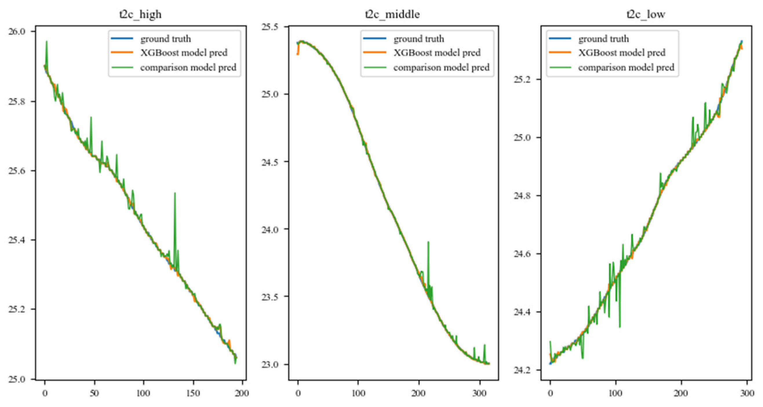
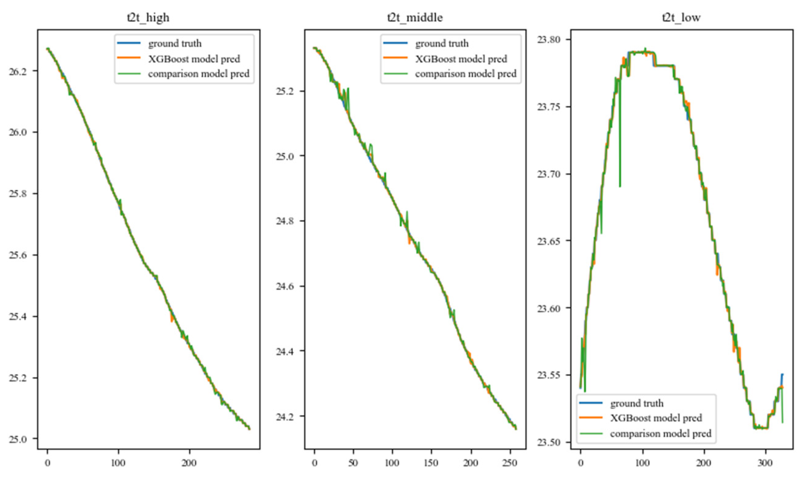
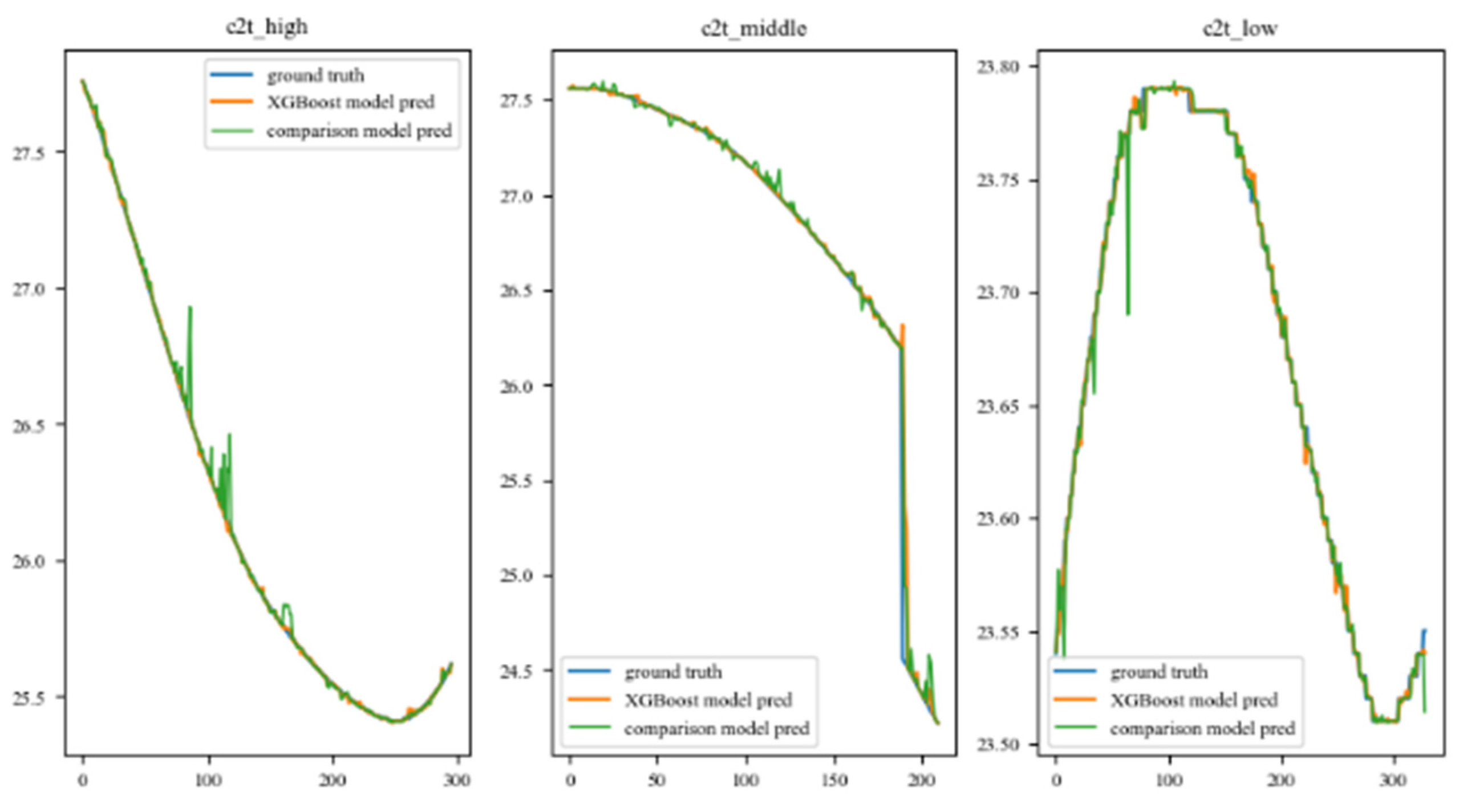
| Model Result | XGBoost Model | Comparison Model * |
|---|---|---|
| MSE | 0.002181 | 0.003530 |
| RMSE | 0.046696 | 0.059411 |
| MAE | 0.017466 | 0.023146 |
| R2 | 0.999927 | 0.999881 |
Disclaimer/Publisher’s Note: The statements, opinions and data contained in all publications are solely those of the individual author(s) and contributor(s) and not of MDPI and/or the editor(s). MDPI and/or the editor(s) disclaim responsibility for any injury to people or property resulting from any ideas, methods, instructions or products referred to in the content. |
© 2024 by the authors. Licensee MDPI, Basel, Switzerland. This article is an open access article distributed under the terms and conditions of the Creative Commons Attribution (CC BY) license (https://creativecommons.org/licenses/by/4.0/).
Share and Cite
Zhu, K.; Yang, X.; Zhang, Y.; Liang, M.; Wu, J. A Heterogeneity-Aware Car-Following Model: Based on the XGBoost Method. Algorithms 2024, 17, 68. https://doi.org/10.3390/a17020068
Zhu K, Yang X, Zhang Y, Liang M, Wu J. A Heterogeneity-Aware Car-Following Model: Based on the XGBoost Method. Algorithms. 2024; 17(2):68. https://doi.org/10.3390/a17020068
Chicago/Turabian StyleZhu, Kefei, Xu Yang, Yanbo Zhang, Mengkun Liang, and Jun Wu. 2024. "A Heterogeneity-Aware Car-Following Model: Based on the XGBoost Method" Algorithms 17, no. 2: 68. https://doi.org/10.3390/a17020068
APA StyleZhu, K., Yang, X., Zhang, Y., Liang, M., & Wu, J. (2024). A Heterogeneity-Aware Car-Following Model: Based on the XGBoost Method. Algorithms, 17(2), 68. https://doi.org/10.3390/a17020068