A Reinforcing-Learning-Driven Artificial Bee Colony Algorithm for Scheduling Jobs and Flexible Maintenance under Learning and Deteriorating Effects

Abstract

In the last decades, the availability constraint as well as learning and deteriorating effects were introduced into the production scheduling theory to simulate real-world case studies and to overcome the limitation of the classical models. To the best of our knowledge, this paper is the first in the literature to address the permutation flowshop scheduling problem (PFSP) with flexible maintenance under learning and deterioration effects to minimize the makespan. Firstly, we address the PFSP with flexible maintenance and learning effects. Then, the deteriorating effect is also considered. Adaptive artificial bee colony algorithms (ABC) enhanced with Q-learning are proposed, in which the Nawaz–Enscore–Ham (NEH) heuristic and modified NEH heuristics are hybridized with a maintenance insertion heuristic to construct potential integrated initial solutions. Furthermore, a Q-learning (QL)-based neighborhood selection is applied in the employed bees phase to improve the quality of the search space solutions. Computational experiments performed on Taillard’s well-known benchmarks, augmented with both prognostic and health management (PHM) and maintenance data, demonstrate the effectiveness of the proposed QL-driven ABC algorithms.

1. Introduction

Scheduling is an important tool for manufacturers and production engineers since it deals with the allocation of human and machine resources to satisfy consumer demand. The objective is to monitor and optimize workloads, as well as to reduce production time and costs while adhering to all production constraints.

In traditional scheduling problems and models, job processing times are assumed to be a constant value. However, this hypothesis is not suitable for many realistic situations in which the job processing time may change owing to job deterioration and/or learning effect phenomena. Indeed, when the employees execute the same task repeatedly, they learn how to perform more efficiently. On the other hand, machines wear out after long periods of processing. Therefore, recent trends in scheduling theory have focused on modeling real-world production scheduling problems where human learning, as well as machine deteriorating effects, are taken into account when studying scheduling problems [1,2]. The learning effect [3] is a natural human-oriented phenomenon appearing among operators after repeating similar tasks frequently. They gain experience and the execution time decreases accordingly. Ref. [4] proposed the first modeling of this phenomenon with a learning curve and since then, multiple models have been proposed in the literature. Refs. [3,5] were among the pioneers that investigated the learning effect in scheduling problems, and this was continued in the literature in hundreds of studies with different machine configurations [6,7]. On the other hand, the deteriorating effect [8,9] is a machine-oriented phenomenon appearing after processing tasks are conducted on machines for a long time. The machine performances wear out and therefore additional delays are required to execute the production schedule. Refs. [8,10] seem to be the first to have investigated this effect in production scheduling. The interested reader can find extensive surveys of different scheduling models and problems involving deteriorating jobs in [11,12]. More recently, Ref. [13] presented an updated survey of the results on scheduling problems with deteriorating jobs and time-dependent processing times. As for learning and/or deterioration effects, Ref. [7] reviews the mathematical models for scheduling problems. It is worth noting that most proposed learning or deteriorating effects functions are either position-dependent, time-dependent, or sum-of-processing-times-dependent [6,13,14].

To counter the deteriorating effect, increase machines’ availability, and reduce the overall production costs, maintenance activities should be planned along the production process [15]. However, unavailability periods for machines appear since the maintenance activities may take up a potential production time that could otherwise be allocated to completing production tasks. Therefore, to compensate for this deficiency, maintenance tasks should be scheduled in an effective way to improve machine availability and minimize disruption to the production process [16]. Ref. [17] established that appropriate maintenance planning can preserve machine performance and save 20–30% of total operating costs.

Recently, maintenance strategies have moved towards a smart aspect. In fact, modern sensor, diagnosis, and prognostic and health management (PHM) technologies allow the ideal planning of interventions and reduce inopportune spending. Simply put, signals gathered from embedded sensors (or inspection information) are analyzed in order to continuously (or periodically) monitor the health state of the production system. Following that, the current state is inferred and the future progression till failure is predicted in order to estimate the time left before the occurrence of failure, known as the remaining useful life (RUL) [18]. Then, the PHM outputs (i.e, RUL) are exploited in the decision making that concerns maintenance planning. The main advantage of this strategy, namely the decision making based on prognosis information, which is referred to as a post-prognostic decision (PPD) [19], is that it maintains the system only when necessary, which reduces the cost of inopportune maintenance interventions.

The current PPD research on scheduling problems is focused on two main streams. First, the intent is to make the best PPD regarding maintenance planning. In order to improve maintenance planning, PHM findings are thus used [20,21,22,23]. On the other hand, the second stream looks into the issue of integrating production jobs and maintenance operations when making decisions. This can help to avoid production downtime and improve system availability by establishing the most appropriate integrated production and maintenance schedule [16,18,24,25,26,27].

Metaheuristics have emerged as a common solution approach for scheduling in industry and manufacturing due to the fact that most problems are computationally hard [28]. Recently, bio-inspired metaheuristics, including evolutionary algorithms and swarm intelligence algorithms, have become increasingly popular [29]. Evolutionary algorithms start with a set of random candidate solutions and iteratively generate descendant solutions until an acceptable one is found. Common metaheuristics in this category that have many applications in scheduling problems are genetic algorithms [30,31], the differential evolution algorithm [32], and more recently, biogeography-based optimization (BBO) [33]. Swarm Intelligence is an advanced artificial intelligence discipline that uses the behavior of living swarms such as ants, bees, butterflies, and birds to solve complex problems [34]. Several metaheuristics in this category have been applied to solve scheduling problems such as Ant Colony Optimization (ACO) [35], Particle Swarm Optimization (PSO) [36], and more recently, Grey Wolf Optimization (GWO [37]). The artificial bee colony (ABC) algorithm [38], which has recently been introduced to formulate NP-hard problems, simulates the social behavior of bees when searching for promising food sources associated with higher nectar amounts. The ABC algorithm has been extensively applied to solve various flowshop scheduling problems [39,40,41]. On the other hand, machine learning (ML) is an expansive field within artificial intelligence that has gained significant popularity due to its straightforward algorithms, enabling programs to learn patterns, behaviors, models, and functions. This acquired knowledge is then utilized to enhance future decision making and actions. ML can be categorized into three main types: supervised learning, unsupervised learning, and reinforcement learning. In recent years, reinforcement learning (RL) methods have been applied to machine scheduling problems [42]. It is noteworthy that among scheduling problems, jobshop scheduling, flowshop scheduling, unrelated parallel machine scheduling, and single-machine scheduling have emerged as the most extensively studied ones [42].

While integrating maintenance decisions in production scheduling problems makes existing models and solution methods more realistic, it also increases their complexity. Furthermore, incorporating effects further increases the problem’s complexity. Additionally, while most research on deteriorating jobs and learning effects has focused on single-machine problems [1], it is the multimachine problems that are more interesting and closer to real-world problems. Therefore, the intent of this paper is to explore the permutation flowshop scheduling problem (PFSP) with flexible maintenance under learning and deteriorating effects, through the perspective of reinforcement learning algorithms. In this regard, we propose two Q-learning (QL)-driven artificial bee colony (ABC) algorithms to solve the defined PFSP with only the learning effect and the defined PFSP with simultaneous consideration of learning and deteriorating effects. The main advantages of the proposed hybrid metaheuristic approaches are the following:

1.

To be close to realistic production workshops, we propose a novel interpretation of PHM outputs, where RULs and degradation values are estimated based on the operating conditions of machines during the processing of production jobs;

2.

The use of the QL algorithm, one of the major RL algorithms, to guide the search process in the employed bees phase of the ABC algorithms;

3.

The design of a new heuristic, named INEH, based on the hybridization of the NEH heuristic [43] and maintenance insertion heuristic [44] concepts, to generate initial solutions of good quality;

4.

A maintenance cost function to be optimized when readjusting maintenance emplacements after being perturbed in employed and onlooker bees phases;

The remainder of this paper is organized as follows. A literature review and the research gaps are given in Section 2. The problem formulation and objective function are provided in Section 3. Section 4 details the proposed ABC-based solving approaches. Section 5 discusses the performance analyses and presents our computational results. Finally, some conclusions and future works are discussed in Section 6.

2. Brief Literature Review and Research Gaps

Scheduling problems are considered to be of very complex resolution. Not only are they NP-complete [45], but they are also actually among the most difficult problems to solve because of the difficulty of computing solutions [46]. The joint scheduling problem addressed in this paper is even more complex as it involves not only assigning production jobs and maintenance activities to machines but also accounting for the impact of learning and deteriorating effects on processing times.

2.1. Metaheuristic Solution Approach

As a result of their efficiency and ability to be used in real-world production environments, metaheuristics as approximation methods have made breakthroughs in solving various complex optimization problems in the industry and become the main methods used to solve large-scale scheduling problems [47]. Nonetheless, it is worth noting that few studies in the literature have proposed metaheuristics to solve scheduling problems with learning and/or deteriorating effects [1,2].

The existing literature can be placed into three main streams according to the considered effect, namely the learning effect, the deteriorating effect, and finally, the combined effects. Reference [48] proposed a tabu search algorithm to solve the single-machine scheduling problem with a time-dependent learning effect. Ref. [49] developed four metaheuristics, namely the genetic algorithm (GA), simulated annealing, ABC, and iterated greedy algorithms to solve a two-stage, three-machine assembly scheduling problem with a position-dependent learning effect. On the other hand, Ref. [41] proposed an ABC algorithm to solve the flexible flowshop scheduling problem with a step deteriorating effect, while [50] proposed three metaheuristics including dynamic differential evolution, the simulated annealing algorithm, and the cloud-theory-based simulated annealing algorithm, to solve the two-stage assembly scheduling problem under a time-dependent deteriorating effect. In practical settings, combined effects (learning and deteriorating) are also considered. In this regard, we can quote the work of [51], which developed a GA to solve parallel machine scheduling problems under the effects of position-dependent learning and time-dependent deteriorating effects.

Joint planning of production and maintenance activities, taking into account learning and/or deteriorating effects has also been studied in the literature. However, works in this area are even more scarce. From the learning perspective, Ref. [52] solved the joint flowshop scheduling problem with a hybrid metaheuristic algorithm based on the simulated annealing algorithm and firefly algorithm. For the deteriorating effect, Ref. [53] developed a GA to deal with the joint single-machine scheduling problem taking into account the deteriorating effect. Finally, considering the case of combined effects, Ref. [54] proposed an ABC algorithm to solve the joint flowshop scheduling problem under the time-dependent deteriorating effect and position-dependent learning effect. Ref. [55] studied the joint parallel batching scheduling problem under a combined position-dependent learning effect and time-dependent deteriorating effect. A hybrid algorithm combining GA and differential evolution (DE) was proposed for resolution.

Based on the findings of the literature, it has been observed that scheduling problems frequently feature position-dependent learning effects and/or time-dependent deteriorating effects [2]. Furthermore, variable maintenance durations due to learning or deteriorating effects is also an important research stream in the scheduling literature. While variable maintenance durations due to the deterioration effect have most often been considered [56,57,58], variable maintenance durations due to the learning effect have scarcely been studied [54,59].

2.2. Metaheuristic and RL Solution Approach

Recently, there has been a growing focus on using reinforcement learning (RL) [60], a class of ML algorithms, as an emerging intelligent optimization method for addressing complex combinatorial optimization problems. The RL algorithms have been successfully applied to solve a wide range of production scheduling problems [42,61]. Ref. [62] proposed a Q-learning (QL) algorithm to solve the classical PFSP. The authors reported competitive results compared to the optimum values proposed in the literature. Ref. [63] applied the QL algorithm to the makespan hybrid flowshop scheduling problem. To validate the method, two real-life applications were made. Ref. [64] proposed a multi-agent reinforcement learning framework for the jobshop scheduling problem. The best results are returned by the approach using well-known benchmark instances.

In the literature, integrating RL algorithms into metaheuristics has been proven to offer high performance in terms of search robustness, solution quality, and convergence speed [42]. Metaheuristics can rely on RL algorithms to calibrate their key parameters [31,65] or support their search process [66,67]. Despite extensive efforts to incorporate RL algorithms into metaheuristics for scheduling problem resolution, little research has addressed constraints such as maintenance, learning, and deteriorating effects [42]. Furthermore, despite the extensive literature on flowshop scheduling problems, to the best of our knowledge, references to the problem addressed in this paper, that is, the PFSP with flexible maintenance under learning and deteriorating effects, are very scarce. Hence, this paper introduces several enhancements to the ABC algorithm based on the specific characteristics of the problem under investigation. These improvements, including the hybrid initialization method and QL-based neighborhood search, aim to improve the search capability and overall performance.

3. Integrated Problem Description and Effects Mathematical Models

In this section, we first describe the integrated permutation flowshop scheduling problem (PFSP) with flexible maintenance that we are dealing with. We focus on the variable duration of maintenance and job processing times due to learning and deteriorating effects. Furthermore, the assumptions made in this paper are provided. Finally, we discuss the most salient aspects of learning and deteriorating effects. The following notations are used for the remainder of this paper:

J	indicates a set of production jobs to be processed.
j	indicates the index of a job in the set J ($1\le j\le n$).
$M_i$	indicates the ith machine, i is used as the machine index ($1\le i\le m$).
$k_i$	indicates the number of planned maintenance operations on machine i.
$M_{ic}$	indicates the planned maintenance operation on machine i at the cth position, where c is used as the maintenance position indicator ($1\le c\le k_i$).
$p_{ij}$	indicates the normal processing time of job j on machine i.
$p_{ij}\left(t\right)$	is the time-dependent deteriorating processing time of job j on machine i, where t is its start time.
$\beta$	is the deteriorating index.
$p{m}_{ic}$	is the normal time of the cth maintenance on machine i.
$p{m}_{ic}\left(c\right)$	is the position-dependent learning time of the cth maintenance on machine i.
$\alpha$	is the learning index.
${\sigma }_{ij}$	indicates the degradation of machine i after processing the job j.
$B_{il}$	indicates a subset of J with $n^{\prime }$ jobs where $n^{\prime }<n$.
$C_{max}$	indicates the total completion time.

3.1. The Integrated Scheduling of Production and Maintenance Problem

The PFSP is one of the most thoroughly studied scheduling problems in the operation research literature. Many production scheduling problems resemble a flowshop, and therefore, it has been extensively studied due to its application in industry [68].

Formally, the PFSP can be described as follows. A set $J=\{j,1\le j\le n\}$ of n independent jobs needs to be processed on a set $M=\{M_i,1\le i\le m\}$ of m independent machines in the same order on the m machines. We assume that all jobs are available at time zero and no preemption is allowed. In order to ensure the system’s reliability and to prevent the occurrence of fatal breakdowns during the processing horizon, machines are monitored continuously by a PHM module. This module is able to predict, for each machine $M_i$, the relative time before failure after processing a job j, noted as $RU{L}_{ij}$, and the resulting degradation value, ${\sigma }_{ij}$, is then deduced. When the cumulative jobs degradation reaches a certain threshold, $\mathsf{\Delta }$, a maintenance operation should be planned.

The resulting integrated sequence is denoted $\Pi =\{{\pi }_1,{\pi }_2,\cdots ,{\pi }_m\}$ where ${\pi }_i$ represents the corresponding integrated sequence of n jobs and $k_i$ ($\ge 1$) flexible maintenance on machine $M_i$. Then ${\pi }_i$ can be seen as a succession of $k_i+1$ blocks of jobs ($B_{il}=\{$subset of $J\}$) separated by maintenance operations ($M_{ic}$):

${\pi }_i$= $\{B_{i1},M_{i1},B_{i2},M_{i2},\cdots ,B_{ik},M_{i{k}_i},B_{i(k_i+1)}\}$, where ${\cup }_{l=1}^{k_i+1}{B}_{il}=J$.

The general assumptions of the integrated problem are given as follows:

• At time zero, all jobs are available and ready for processing and no preemption is allowed;
• Each machine can handle at most one action (production or maintenance) and each job can be processed by at most one machine;
• Each production job j (maintenance operation $M_{ic}$) requires a basic amount of processing time on each machine i, represented by $p_{ij}$ ($p{m}_{ic}$);
• We fix the degradation value associated to job j after being processed on machine i, ${\sigma }_{ij}=p_{ij}/RU{L}_{ij}$ where $0<{\sigma }_{ij}<1$.
• The maximal authorized threshold degradation $\mathsf{\Delta }$ is fixed to 1 for all machines;
• At least one maintenance intervention is performed on each machine and no maintenance intervention is performed after the processing of the last job;
• After a maintenance intervention, the machine is recovered to an “As good as new” state.

3.2. Learning and Deteriorating Effects’ Mathematical Models

Due to the learning effect, we suppose that the maintenance durations will decrease gradually as they are scheduled later in the sequence. This is the position-dependent learning model (Equation (1)). On the other hand, for the deteriorating effect, we suppose that the production job processing times will increase gradually over time. This is the time-dependent deteriorating model (Equation (2)).

$$p{m}_{ic}\left(c\right)=p{m}_{ic}\times c^{\alpha },-1<\alpha <0$$

(1)

$$p_{ij}\left(t\right)=p_{ij}+\beta \times t,\beta >0$$

(2)

4. Proposed QL-Driven ABC-Based Solving Approaches

The ABC algorithm [38] is a competitive bio-inspired algorithm that simulates the behavior of bee colonies when searching for promising food sources associated with higher nectar amounts. In the ABC algorithm, the food source represents a candidate solution to the problem and the nectar amount of a source corresponds to the quality, known as fitness, of the related solution. The ABC search process is conducted by three bee swarms, namely: employed, onlooker, and scout bees. A review of its fundamentals and some applications can be found in [69]. In [70], the ABC algorithm showed effective performances over the differential evolution (DE) algorithm, Particle Swarm Optimization (PSO), and evolutionary algorithm (EA). The main advantages of the ABC algorithm are its ability to balance exploitation and exploration, it having few control parameters, its fast convergence, its strong robustness, and its ease of being combined with other methods [71]. It is also easy to implement compared to GA and Ant Colony Optimization (ACO) [72].

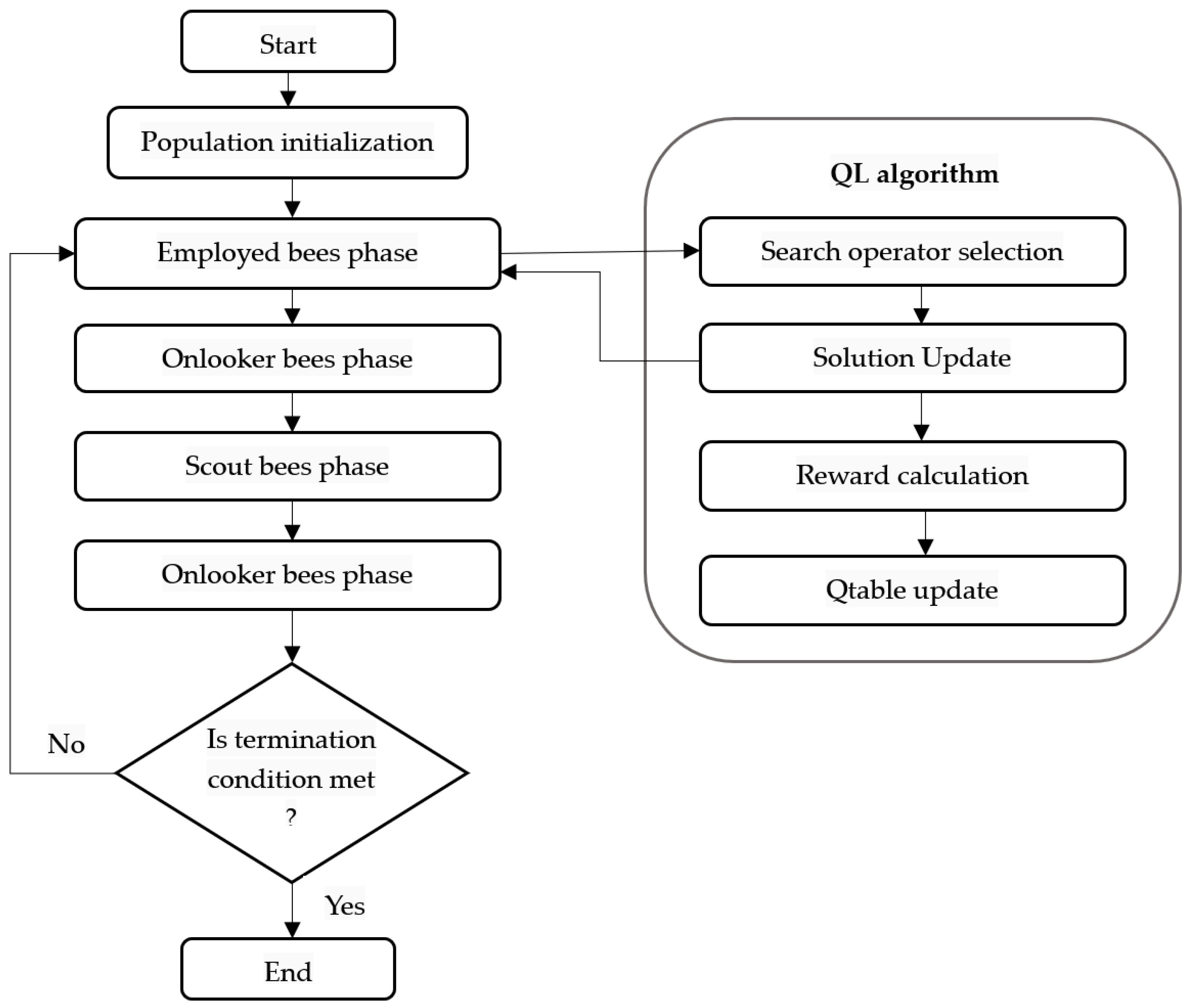
In an attempt to solve the integrated PFSP with a flexible maintenance problem under learning and deteriorating effects in a reasonable time, in this paper, we propose two efficient ABC algorithms enhanced with the RL mechanism. The first ABC algorithm, named IQABC-LE for Integrated QL-based ABC under Learning Effect, takes into account the learning effect. After generating the initial solutions, the search process of IQABC-LE starts with the employed bees phase, which applies an RL mechanism to drive the neighborhood exploitation of the associated solutions in order to update the search space with optimal solutions. After that, the onlooker bees select the best individuals from the search space to exploit their neighborhood for further optimization. To allow exploration of the search space, the scout bees randomly replace the solutions that have not been updated after a defined number of trials. The search process is iterated until a termination condition is met. The general scheme of the IQABC-LE algorithm is given in Algorithm 1 and its flow chart is indicated in Figure 1. The second ABC algorithm, named IQABC-LDE for Integrated QL-based ABC under Learning and Deteriorating Effects, follows the same steps as IQABC-LE but also takes into account the deteriorating effect. The main features of the proposed algorithms are detailed in the sections below.

4.1. Food Source Representation and Evaluation

A suitable solution representation is based on the work of [73]. A candidate solution $Sol$, i.e., food source, jointly specifies the production job sequence and the maintenance operations’ positions on each machine and is codded by a two-field structure. The first field is a vector S = $\{j,j\in [1,n\left]\right\}$ representing the production job order. The second field represents the scheduling of maintenance operations on each machine by a binary matrix P of $m\times n$ size. An element $P\left[\begin{array}{c}i,j\end{array}\right]$ of P indicates if a maintenance intervention is scheduled on machine $M_i$ after job j, and then $P\left[\begin{array}{c}i,j\end{array}\right]$=1, or not, and then $P\left[\begin{array}{c}i,j\end{array}\right]$=0. Let

$\mathrm{S} = \left(\begin{array}{cccccccccc}1\hfill & 9& 3& 8& 5& 6& 7& 4& 2& 0\end{array}\right),$ and

$P=\left(\begin{array}{ccccccccc}0\hfill & 1& 0& 0& 1& 0& 0& 0& 1\\ 0& 0& 1& 0& 0& 1& 0& 0& 0\\ 0& 1& 0& 0& 0& 1& 0& 0& 0\end{array}\right)$

represent a solution of an integrated flowshop scheduling problem with $m=3$ machines and $n=10$ jobs. Then, the execution order of the ten jobs and maintenance operations on the three machines is the following:   

Machine 1: 1, 9, M${}_{11}$, 3, 8, 5, M${}_{12}$, 6, 7, 4, 2, M${}_{13}$, 0.

Machine 2: 1, 9, 3, M${}_{21}$, 8, 5, 6, M${}_{22}$, 7, 4, 2, 0.

Machine 3: 1, 9, M${}_{31}$, 3, 8, 5, 6, M${}_{32}$, 7, 4, 2, 0.

Algorithm 1: IQABC-LE()

Require:  Population size (PopSize), Onlooker bees percentage (onlook%), Number of generations (max_iterations), Abandonment number of trials (limit) Begin $Ebees\left[1\right]\leftarrow INEH\left(\right)$                                       ▹ Population initialization step for $i\leftarrow 1$ to alpha%PopSize do     $Ebees\left[i\right]\leftarrow ModifiedNeh\left(\right)$ end for for $j\leftarrow 1$ to (PopSize-alpha%PopSize-1) do     $Ebees\left[j\right]\leftarrow RandomGeneration\left(\right)$ end for $iter\leftarrow 1$ while $iter\le max\_iterations$ do     for $i\leftarrow$1 to PopSize do                                      ▹ employed bees phase         NeighborEbee← QL(Ebees[i])                                   ▹ Qlearning selection (Algorithm 3)         if NeighborEbee ≥ Ebees[i] then            Ebees[i]← NeighborEbee         end if     end for     for i←1 to onlook%PopSize do                                     ▹ onlooker bees phase         Olook[i]← probaSelection(Ebees)         Olook ← ILS(Olook[i])         if Olook ≥ Olook[i] then            Ebees[i]←Olook         end if     end for     for i←1 to PopSize do                                         ▹ scout bees phase         if CheckLimit(Ebees[i],limit)=True then            Ebees[i]←RandomGeneration()         end if     end for end while Return Best Solution() End

The objective is to find a solution $Sol$ that minimizes the amount of nectar (the measure of the quality of a solution), i.e., the best sequencing of jobs and maintenance operations to be processed for each machine in order to minimize the total completion time of the schedule, $C_{max}$, taking into account maintenance interventions planning under learning and deteriorating effects. Considering the learning and the deteriorating effects, and the fact that the total completion time $C_{max}$ depends mainly on the sum of the job processing times and maintenance durations (see Formula (3)), the $C_{max}$ while considering the learning effect and both effects simultaneously are given by Formulas (4) and (5), respectively.

$$C_{max}=IT+{\mathsf{\Sigma }}_{j=1}^{j=n}{p}_{mj}+{\mathsf{\Sigma }}_{c=1}^{c=k_m}p{m}_{mc}$$

(3)

$$C_{max}=IT+{\mathsf{\Sigma }}_{j=1}^{j=n}{p}_{mj}+{\mathsf{\Sigma }}_{c=1}^{c=k_m}p{m}_{mc}\left(c\right)=IT+{\mathsf{\Sigma }}_{j=1}^{j=n}{p}_{mj}+{\mathsf{\Sigma }}_{c=1}^{c=k_m}(p{m}_{mc}\times c^{\alpha })$$

(4)

$$C_{max}=IT+{\mathsf{\Sigma }}_{j=1}^{j=n}{p}_{mj}\left(t\right)+{\mathsf{\Sigma }}_{c=1}^{c=k_m}p{m}_{mc}\left(c\right)=IT+{\mathsf{\Sigma }}_{j=1}^{j=n}(p_{mj}+\beta \times t)+{\mathsf{\Sigma }}_{c=1}^{c=k_m}(p{m}_{mc}\times c^{\alpha })$$

(5)

where: $IT$ refers to the total idle time of the last machine m waiting for jobs arrival and $k_m$ is the number of inserted maintenance activities on the last machine m.

4.2. Initial Population Generation

To allow quality and diversity in the search space, we generated an initial population of candidate solutions at random and “seeded” it with some good ones. Therefore, in this work, we suggest the following three-step initialization procedure to generate an initial population of $PopSize$ complete integrated solutions ($S,P$):

• Step 1. Firstly, we generated the first candidate food source of the initial population with a newly designed heuristic, named INEH, a greedy approximate heuristic based on the well-known NEH heuristic [43], by modifying its second phase.
• Step 2. Generate $\alpha \%$ PopSize production sequences using a modified NEH heuristic [74]. To generate complete food sources, maintenance activities are scheduled using the PHM-based greedy heuristic of [44]. In this heuristic, maintenance operations are inserted according to the current accumulated degradation of the machine estimated by the PHM module, starting from the first machine $M_1$ to the last one $M_m$.
• Step 3. The rest of the population is generated randomly with production sequences generated at random and maintenance operations inserted using the heuristic of [44].

The main idea of the INEH heuristic is to build from scratch the sequence of production jobs and maintenance operations giving priority to jobs with higher processing times to be scheduled first. In the first phase, the jobs are ordered according to the LPT rule in a list L. Then, a partial sequence is generated with the first job of L. The second phase is an insertion procedure to iteratively construct a complete integrated sequence. This phase starts first, by scanning the current partial sequence, and maintenance operations are inserted when necessary with respect to the threshold $\mathsf{\Delta }$=1 on each machine. Then, by testing the second job of L in all available positions of the integrated partial sequence. The position that yields the minimum makespan is chosen to be inserted, and the new partial integrated sequence overwrites the last one. This insertion step is repeated iteratively with the rest of the jobs. Detailed steps of the INEH heuristic are given in Algorithm 2.

Algorithm 2: INEH Heuristic

Require:  A Set of production jobs Begin Let L the list of ranked production jobs in decreasing order of total processing time (LPT rule). Insert the first job of L in the first position of the current partial empty sequence. Update L whileL not Empty do     Insert maintenance operations in the appropriate positions of the current partial sequence with respect to the threshold $\mathsf{\Delta }$     Insert the first job of L in all the k+1 possible positions of the current partial sequence     Evaluate all of k+1 resulting partial sequences     Keep the best sequence as a new current partial sequence     Update L end while Return Integrated sequence End

4.3. QL-Based Employed Bees Phase

RL studies the sequential decision process of interaction between the agent and the environment [75]. Q-learning (QL) is one of the major RL algorithms that allows agents to learn an optimal policy through trial and error in an unknown environment. It does not rely on prior knowledge of the environment’s dynamics [76]. The algorithm uses a value function called the Q-$function$ to estimate the expected cumulative reward for taking specific actions in certain states and following the optimal policy thereafter.

During the learning process, the agent explores the environment, taking actions and observing the resulting rewards and next states. These experiences are used to iteratively update the Q-values, which represent the estimated quality of actions in different states. The update process is guided by the Bellman equation, which relates the current Q-value to the expected future Q-values.

Motivated by the above consideration, this paper introduces the QL principle to the selection of neighborhood structures in order to guide the search process in the employed bees phase of the proposed IQABC algorithms. Employed bees are in charge of searching for new and hopefully better food sources. To this end, in the original ABC algorithm, each employed bee generates one new candidate solution in the neighborhood of the current solution in one food source. The new candidate replaces the old solution if it is better. In this paper, each employed bee is placed on a solution from the population and applies one of the neighborhood structures on it, to generate a new solution. The choice of the neighborhood structure is performed by the application of a QL algorithm. The new solution replaces the current one if its quality is better, otherwise, a non-optimization trials counter, nb_trials, is incremented.

4.3.1. Neighborhood Structures

Neighborhood structures are designed for further optimization of the initial solutions. Based on previous studies on scheduling, it has been found that the insert neighborhood is generally more effective for the PFSP [77]. Furthermore, it is advised to incorporate complementary neighborhood structures to ensure a thorough exploration of the search space and enhance the effectiveness of the search process. Therefore, in this paper, insert and swap neighborhoods are used. These neighborhood structures allow the generation of new solutions by changing the execution order of production jobs. Additionally, a third type of neighborhood structure involving the shifting of maintenance tasks is utilized. Based on these neighborhoods, six local search operators are proposed as follows:

1.

Swap move on production jobs. It consists of swapping the positions of two production jobs selected randomly from the production sequence.

2.

Double swap move on production jobs. It consists of making two consecutive swap moves on the production sequence.

3.

Insert move on production. It consists of selecting a production job randomly and then inserting it into another randomly selected position in the production sequence.

4.

Double insert move on production jobs. It consists of making two consecutive insert moves.

5.

Right shift move on maintenance activities. It consists of selecting a maintenance operation in a selected machine and then shifting it to the right, i.e., after the next job in the sequence.

6.

Left shift move on maintenance activities. It consists of selecting a maintenance operation in a selected machine and then randomly shifting it to the left, i.e., before the previous job in the sequence.

4.3.2. Q-Learning Algorithm

In the proposed IQABC algorithms, a QL algorithm is used to guide the choice of the neighborhood structures in the employed bees phase. The states of the QL model are defined by the set of population individuals, while the six neighborhood structures indicate the set of actions. At each iteration, the QL agent observes the current solution (s), selects an action (a) (a neighborhood structure), which generates a new solution (s’), and consequently, it receives a reward/penalty (r) signal according to the quality of the generated solution (see Formula (6)). The agent records its learning experience by a Q-value (Q(s,a)), which is stored in a Q-table. The update of the Q-value is given in Formula (7), where ${\alpha }_{ql}$ is the Q-learning rate and $\gamma$ is the discount factor.

$$r=1+C_{max}\left(S\right)-C_{max}\left(S^{\prime }\right)$$

(6)

$$Q(s,a)=Q(s,a)+{\alpha }_{ql}\times (r+\gamma \times \underset{a^{\prime }}{max}Q(s^{\prime },a^{\prime })-Q(s,a))$$

(7)

The action selection mechanism is implemented using an $ϵ$-greedy strategy, where the agent can choose the best action considering the associated Q-value (exploitation), or can select one action randomly (exploration) with an $ϵ$ probability. Thus, the e-greedy strategy enables both exploitation and exploration. That is, the agent has to exploit what it already knows to obtain a reward, but it also needs to explore in order to make better action selections in the future. The employed bees stage with the QL algorithm is recalled in Algorithm 3.

Algorithm 3: QL-based Employed bees phase

Require:  Search space, Q-table of the population Begin for Each solution S from the search space do                       ▹ S is the current state     Generate a random number a     if $a\le ϵ$ then         Choose the best action (Neighbor structure $NS$) associated with the best Q-value of the Q-table.     else         Choose the best action $NS$ randomly     end if     Generate New Solution Sol’ using $NS$                         ▹ Sol’ is the next state end for r← 1+makespan($Sol$)-makespan($So{l}^{\prime }$)                            ▹ reward formula Update the Q-value of the tuple ($Sol$,$NS$) as specified in Formula (7) if makespan($So{l}^{\prime }$) ≤ makespan($Sol$) then     Replace $Sol$ with $So{l}^{\prime }$ end if update the search space End

To implement the QL algorithm, we used the “pandas” python library. The Q-table is stored in a DataFrame structure, which is a two dimensional table where indexes (lines) point to food sources as represented in Section 4.1, and columns refer to a defined list of neighborhood structures as presented in Section 4.3.1.

4.4. Onlooker Bees Phase

Similar to the employed bees phase, the onlooker bees phase aims to enhance the intensification of the local search process. Firstly, the onlooker bees select candidate solutions from the employed bees stage according to the roulette wheel method. Then a local search heuristic borrowed from the iterated local search (ILS) algorithm [78] with destruction and reconstruction procedures is applied to selected solutions for exploitation. The probability that a solution (Sol${}_i$) is allowed to be selected is defined in Formula (8).

$$P\left(So{l}_i\right)=\frac{fitness\left(So{l}_i\right)}{{\sum }_{k=1}^{n}fitness\left(So{l}_k\right)}$$

(8)

4.5. Scout Bees Phase

In the scout bees phase, candidate solutions that have not been updated after a defined number of trials, let this be limit, are abandoned and replaced by new random ones.

4.6. Readjustment Procedure for Maintenance Cost Minimization

The perturbations on the candidate solutions, through the neighborhood structures within the employed bees stage, and the local search heuristic within the onlooker bees phase may disturb the positions of the required maintenance interventions, which can either be advanced or delayed. In both cases, a maintenance cost needs to be considered. An early maintenance intervention is detected when the cumulative degradation caused by the production jobs scheduled before it is less than the threshold $\mathsf{\Delta }$. In this case, we define the maintenance cost as follows:

$$maint\_cost=200\times |\mathsf{\Sigma }\sigma -\mathsf{\Delta }|+100$$

In the case of tardy maintenance intervention, i.e, when the cumulative degradation caused by the production jobs scheduled before it is greater than the threshold $\mathsf{\Delta }$, we define the maintenance cost as follows:

$$maint\_cost=400\times |\mathsf{\Sigma }\sigma -\mathsf{\Delta }|+100$$

An optimal maintenance cost is reached when the cumulative degradation is equal to $\mathsf{\Delta }$.

In this regard, we propose to apply a readjustment procedure (Algorithm 4) after the generation of new solutions in the employed and onlooker bees phase that browses complete solutions to detect early/tardy maintenance interventions and tries to readjust them in the appropriate positions that optimize the maintenance cost.

Algorithm 4: Readjustment procedure

Require:  Sol (a returned solution with job permutation vector S and the associated maintenance matrix P), $\mathsf{\Sigma }\sigma$ the cumulative machine degradation. Begin $\mathsf{\Sigma }\sigma \leftarrow 0$ for Each machine $M_i(i\le m$) do     $\mathsf{\Sigma }\sigma \leftarrow 0$     for Each job j from S do         $\mathsf{\Sigma }\sigma \leftarrow \mathsf{\Sigma }\sigma +{\sigma }_{ij}$         if P[i,j]=1 then            $\mathsf{\Sigma }\sigma \leftarrow 0.$         end if         if $\mathsf{\Sigma }\sigma \ge \mathsf{\Delta }$ then            Insert the maintenance before or after j in order to minimize the maintenance cost.            Update the matrix P with the maintenance emplacement.            Remove the next maintenance: P[i,(next maintenance position)]$\leftarrow 0$.            $\mathsf{\Sigma }\sigma \leftarrow 0$.         end if     end for end for End

4.7. Termination Condition

The termination condition of the proposed IQABC is a maximum number of iterations (max_iterations) of the algorithm or when the limit of the number of iterations without improving the best solution (stagnation) is reached.

5. The Computational Results and Analysis

In this section, the performance of the designed QL-driven ABC algorithms IQABC-LE and IQABC-LDE is demonstrated through numerical experiments on a well-designed test bed. The experiments are conducted in Python 3.9.5 on a personal computer with Windows 10 operating system, Intel i5 CPU (2.10 GHz), and 8-GB RAM.

In the following, we first describe how test data are generated. Secondly, to analyze the performance of our newly proposed algorithms, we conducted two sets of experiments. In the first set, the calibration process, and a comparison between IQABC without learning and deteriorating effects and a standard ABC were performed. In the second, we validated our IQABC algorithms with effects, namely IQABC-LE and IQABC-LDE, by comparing them with several representative algorithms. We ran, independently, all the algorithms five times on each instance. The complete details are reported in the next sections.

5.1. Data Generation

We used two types of data to assess our proposed methods. The first was about production, while the second was about PHM and maintenance data. For the first type, we ran our experiments on a set of 110 known Taillard instances [79] of different sizes (n × m), with n ∈ {20,50,100,200} and m ∈ {5,10,20}. To complete the production data with the PHM data and the maintenance duration, we proceeded as follows:

• For each instance, we generated three levels of machines’ degradation: (1) from the uniform distribution $\mathcal{U}[0.02;0.03]$ for job processing times below 20; (2) from the uniform distribution $\mathcal{U}[0.03;0.06]$ for job processing times between 20 and 50; and from the uniform distribution $\mathcal{U}[0.06;0.1]$ for job processing times above 50.
• Each instance was tested twice, the first time with medium maintenance durations generated from the uniform distribution $\mathcal{U}[50,100]$, designated as the first maintenance mode $M1$, and the second time with long maintenance durations generated from the uniform distribution $\mathcal{U}[100,150]$, designated as the second maintenance mode $M2$.

It is challenging to make a fair comparison between our results and those of other authors. This difficulty arises from the fact that only a small number of authors have addressed the same problem with the same constraints and objectives, and even fewer with the same instances for comparison purposes. Therefore, to demonstrate the effectiveness of our newly proposed QL-driven ABC algorithms, we report the Average Relative Percentage Deviations (ARPD) provided by each algorithm (after maintenance operations) with respect to the best-known solution for the Taillard instance without maintenance operations (see Equation (9)). Taillard’s acceleration technique [80] was applied to compute the makespan. It allows the CPU time to be reduced by calculating all the partial schedules in a given iteration in a single step.

$$ARPD=\frac{1}{R}\times {\mathsf{\Sigma }}_{i=1}^R\frac{C_{max}^{So{l}_i}-C_{max}^{best}}{C_{max}^{best}}\times 100.$$

(9)

where $C_{max}^{best}$ is Taillard’s best-known solution and $C_{max}^{So{l}_i}$ is the returned value, and R is the number of similar scaled instances running.

5.2. IQABC Features Analysis

For the first set of experiments, we undertook a sensitive performance analysis of our newly proposed algorithms IQABC by varying different parameters. These parameters were experimentally found to be good and robust for the problems tested. We chose a full factorial design in which all possible combinations of the following ABC factors were tested:

• Population size PopSize: three levels (50, 70, and 100);
• Onlooker bees percentage onlook%: three levels (20%, 30%, and 40%);
• Abandonment number of trials limit: three levels (5, 10, and 50);
• Number of iterations max_iterations: three levels (100, 150, and 200).

All the cited factors resulted in a total of 3 × 3 × 3 × 3 = 81 different combinations run on a set of $n\times m$ Taillard instances with $n\in \{20;70;120;170;220\}$ and $m\in \{5;10;15;20\}$. The job processing times of the instances were generated uniformly in the interval $[1,99]$, and maintenance durations were generated according to the first maintenance mode (M1) described in Section 5.1. Each instance was executed five times, which meant a total of 16,200 executions. The ARPD was calculated as a response variable. The resulting experiment was analyzed by means of a multifactor analysis of variance (ANOVA) technique [81] with the least significant difference (LSD) intervals at the 95% confidence level.

Each parameter was set to its most adequate level as follows: PopSize = 70; onlook% = 40%; Limit = 5; and max_iterations = 200.

For the QL factors, namely the Q-learning index ${\alpha }_{ql}$, the discount factor $\gamma$, and the probability for the QL mechanism $ϵ$, based on the study of [82], four typical combinations for the QL algorithm were tested:

• C1: $\alpha$ = 0.1, $\gamma$ = 0.8, $ϵ$ = 0.2;
• C2: $\alpha$ = 0.1, $\gamma$ = 0.8, $ϵ$ = 0.1;
• C3: $\alpha$ = 0.1, $\gamma$ = 0.9, $ϵ$ = 0.1;
• C4: $\alpha$ = 0.1, $\gamma$ = 0.9, $ϵ$ = 0.2.

After executing different experiments for each combination, we decided to keep the second combination, as it was able to report better results. Finally, the stagnation factor was set at 80% since a large number of convergence curves for multiple executions showed a stabilization of the results up to this value.

5.3. Performance Analysis of IQABC Algorithm without Learning and Deteriorating Effects

To prove the performance of the integrated QL-driven ABC algorithm without learning and deterioration effects (IQABC), we compared it with three different competing algorithms for the same problem and constraints without considering the learning and deteriorating effects. The comparative algorithms are: (1) a population-based metaheuristic, which is the ABC algorithm of [54] with random neighborhood selection; (2) a unique solution-based metaheuristic, which is the Variable Neighbor Search (VNS) algorithm of [83]; (3) and finally, INEH, our newly designed constructive heuristic. The comparison was carried out by means of 1100 runs of the test benchmark. The resulting ARPD values reported in

Table 1. Performance offset from Taillard’s upper bounds of IQABC, ABC, VNS, and INEH algorithms for maintenance mode 1 and 2.

Instance	M1				M2
	ABC	VNS	INEH	IQABC	ABC	VNS	INEH	IQABC
20x5	4.69	11.52	6.77	3.11	3.43	10.61	8.87	3.34
20x10	13.34	23.01	16.22	11.45	13.97	24.20	19.09	12.33
20x20	25.35	28.19	27.31	23.16	27.03	32.98	29.46	24.84
50x5	2.02	1.72	2.66	0.54	2.83	1.93	2.83	−0.001
50x10	9.93	8.24	12.11	5.91	12.62	9.95	15.79	6.91
50x20	19.79	18.5	21.94	15.12	24.65	19.28	25.01	16.93
100x5	1.16	1.35	1.47	0.93	1.40	1.46	1.93	0.96
100x10	4.34	5.09	5.56	2.90	6.37	5.48	10.27	3.82
100x20	13.41	15	17.36	11.40	16.31	15.61	21.53	13.22
200x10	1.77	3.13	3.10	1.94	2.58	3.43	6.45	2.68
200x20	7.31	11.21	12.6	6.58	9.53	12.55	16.92	8.94
500x20	2.99	-	-	3.08	2.98	-	-	3.64
average	8.84	11.54	11.55	7.18	10.30	12.50	14.38	8.13

were calculated based on the $C_{max}$ value given in Formula (3), with no consideration of the learning and deteriorating effects, and with respect to the first and second maintenance modes ($M1$ and $M2$).

Table 1 shows that the INEH heuristic produces competitive ARPD results compared to the VNS metaheuristic, even though the INEH is a constructive method. In fact, for small instances (20x5, 20x10, 20x20), INEH achieves the best ARPD values: for Mode 1, an average of 16.76 against 20.90 for VNS; for Mode 2, an average of 19.14 for INEH against 22.59 for VNS. Nonetheless, it fails to reach the results obtained by the VNS algorithm for large instances (50x5–200x20): for Mode 1, an average of 9.60 against 8.03 for the VNS; and for Mode 2, an average of 12.59 for INEH against 8.71 for VNS. The great advantage of the INEH heuristic is its ability to obtain near-optimal solutions in a reasonable computation time (on average 6.99 time units (TU) compared to 3120.89 TU for VNS).

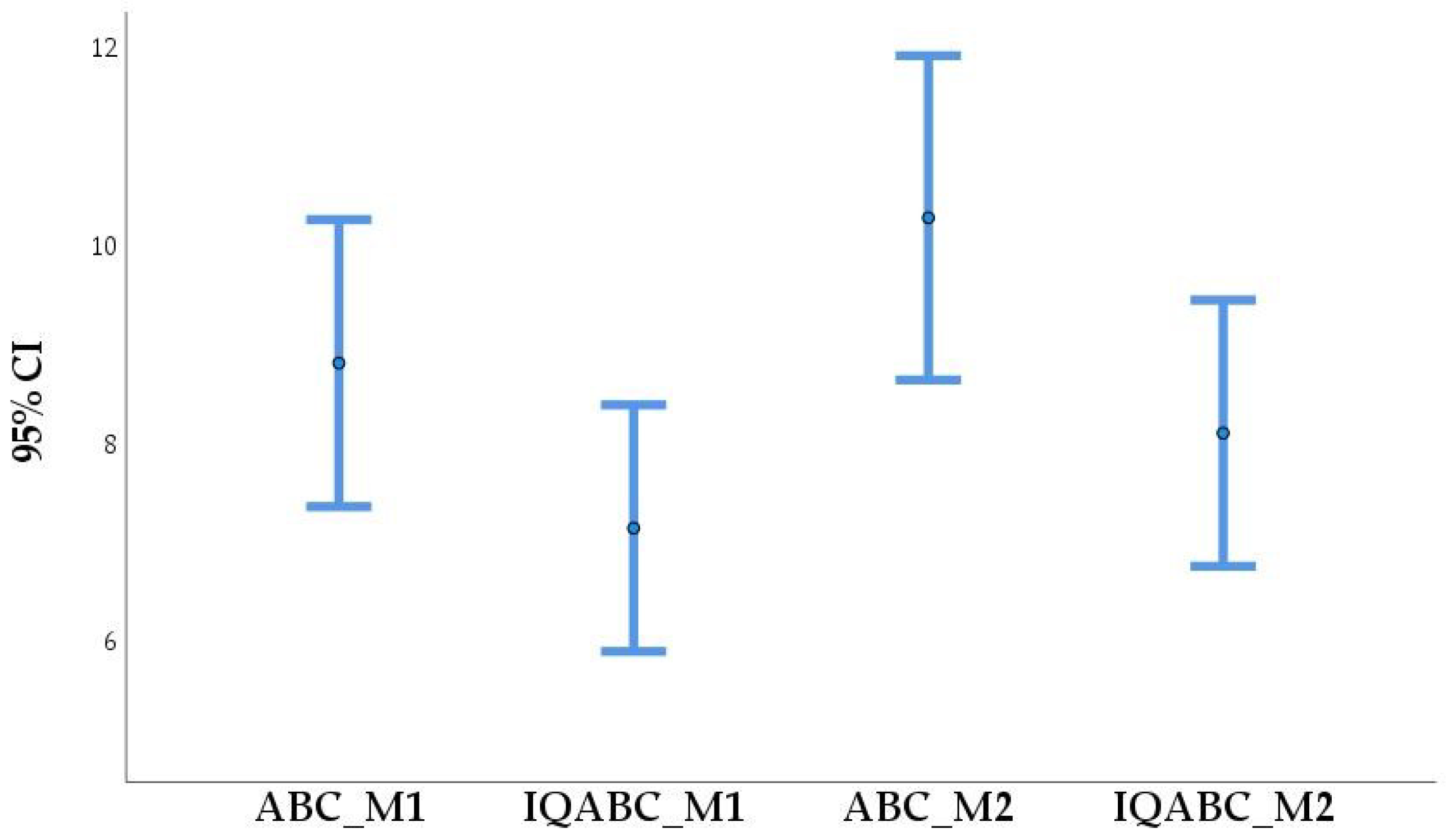
Although the ABC metaheuristic of [54] gave better solutions than the VNS algorithm, which is considered an efficient metaheuristic for the problem [83,84], the IQABC algorithm outperforms it, as can clearly be seen from Table 1 for the two maintenance modes. This is proved by the employed bees’ local search procedures and the QL-driven neighborhood selection. To further verify the statistical significance of the difference in ARPD values between ABC and IQABC for the two maintenance modes, we performed a Friedman’s two-way analysis of variance test [85]. The result summary in

Table 2. IQABC-ABC Friedman’s two-way analysis of variance summary for M1 (left) and M2 (right).

M1		M2
Total N	120	Total N	120
Test statistic	36,300	Test statistic	28,033
Degree of freedom	1	Degree of freedom	1
Asymptotic sig	<0.001	Asymptotic sig	<0.001
Decision	Reject the null hypothesis	Decision	Reject the null hypothesis

as well as the mean plots displayed in Figure 2 show the significant differences between IQABC and ABC. Therefore, the IQABC algorithm is significantly superior to the ABC, VNS, and INEH algorithms. However, the ABC and IQABC algorithms are population-based methods, which means an important amount of time is used to effectively explore the search space. Furthermore, the QL mechanism in the IQABC algorithm needs more time to learn optimal policies. Therefore, it is not meaningful to compare the running times of the IQABC and ABC algorithms with those of the VNS and INEH heuristics.

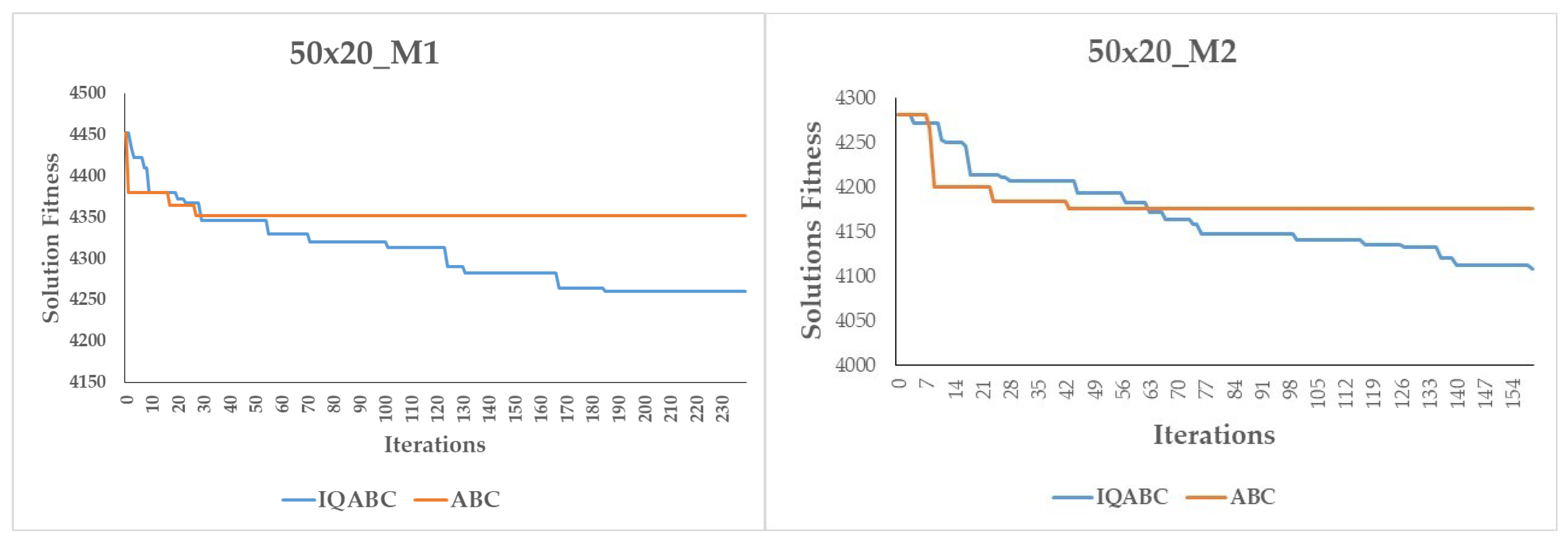
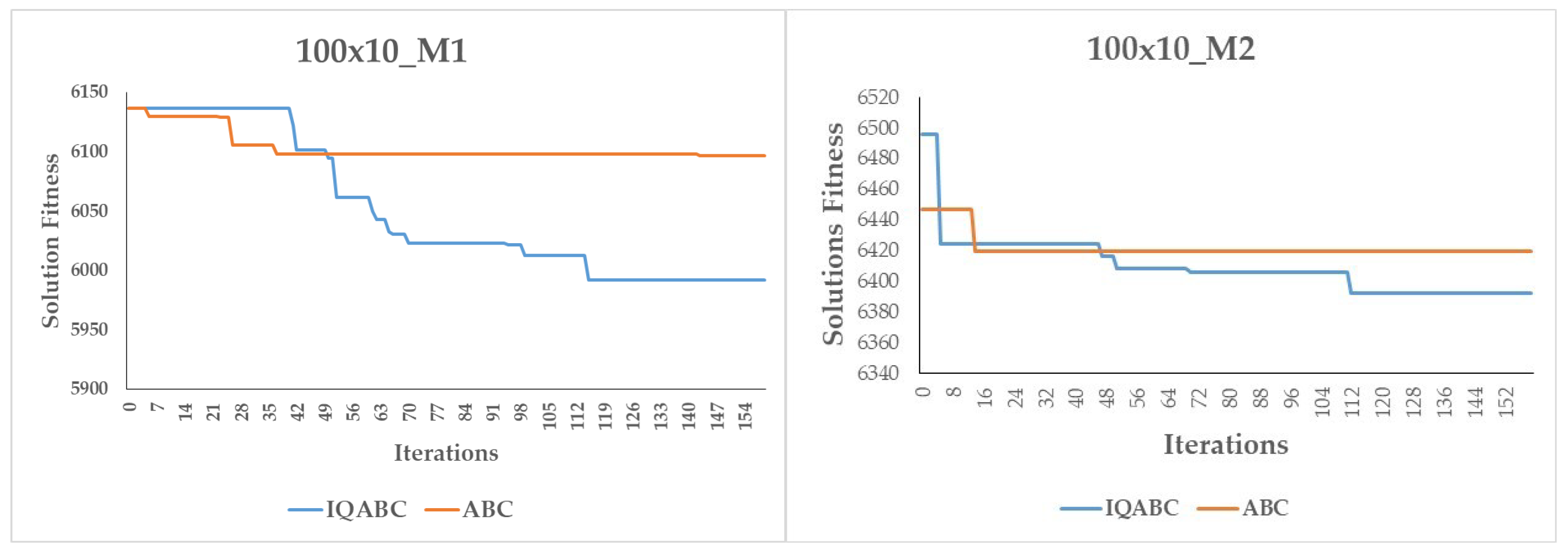
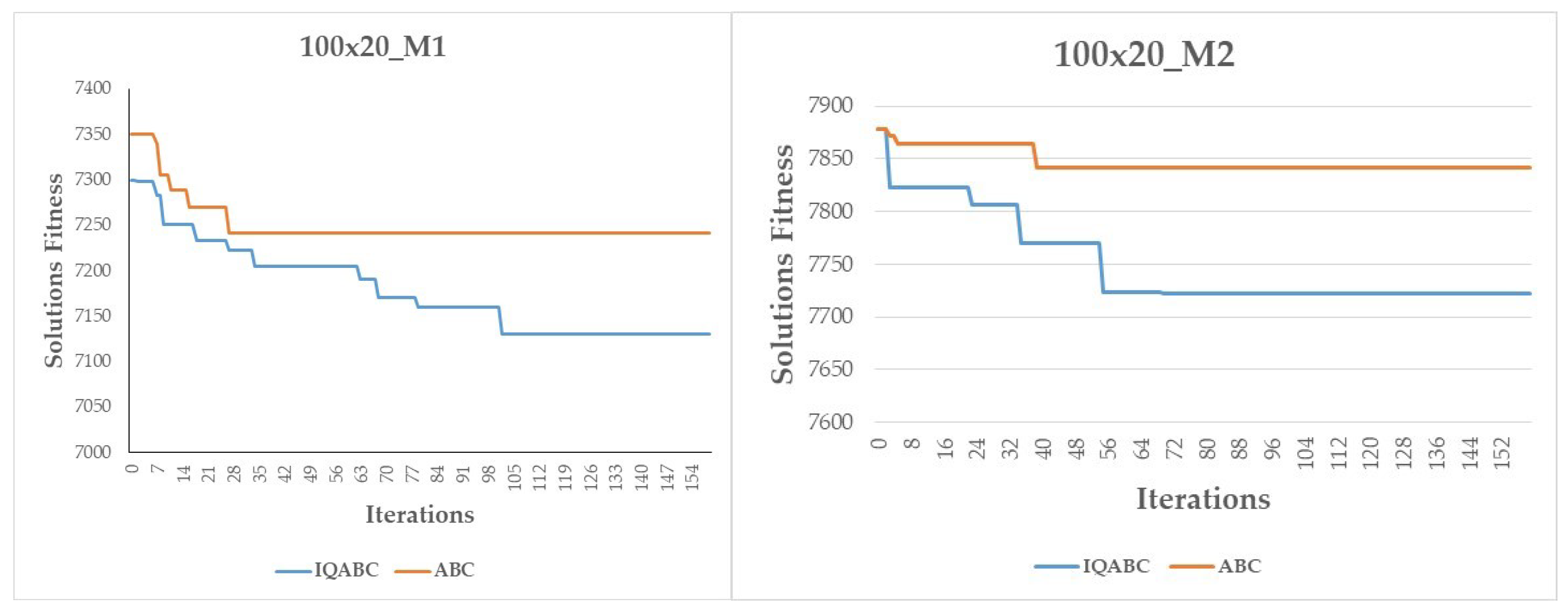
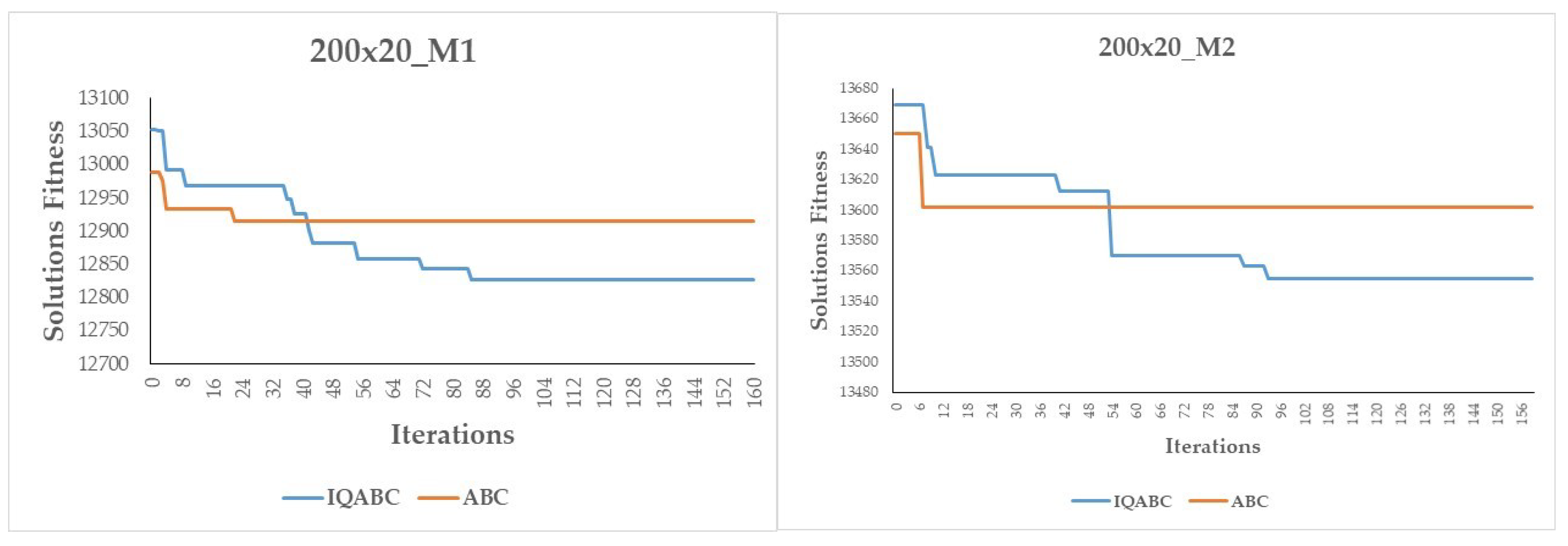
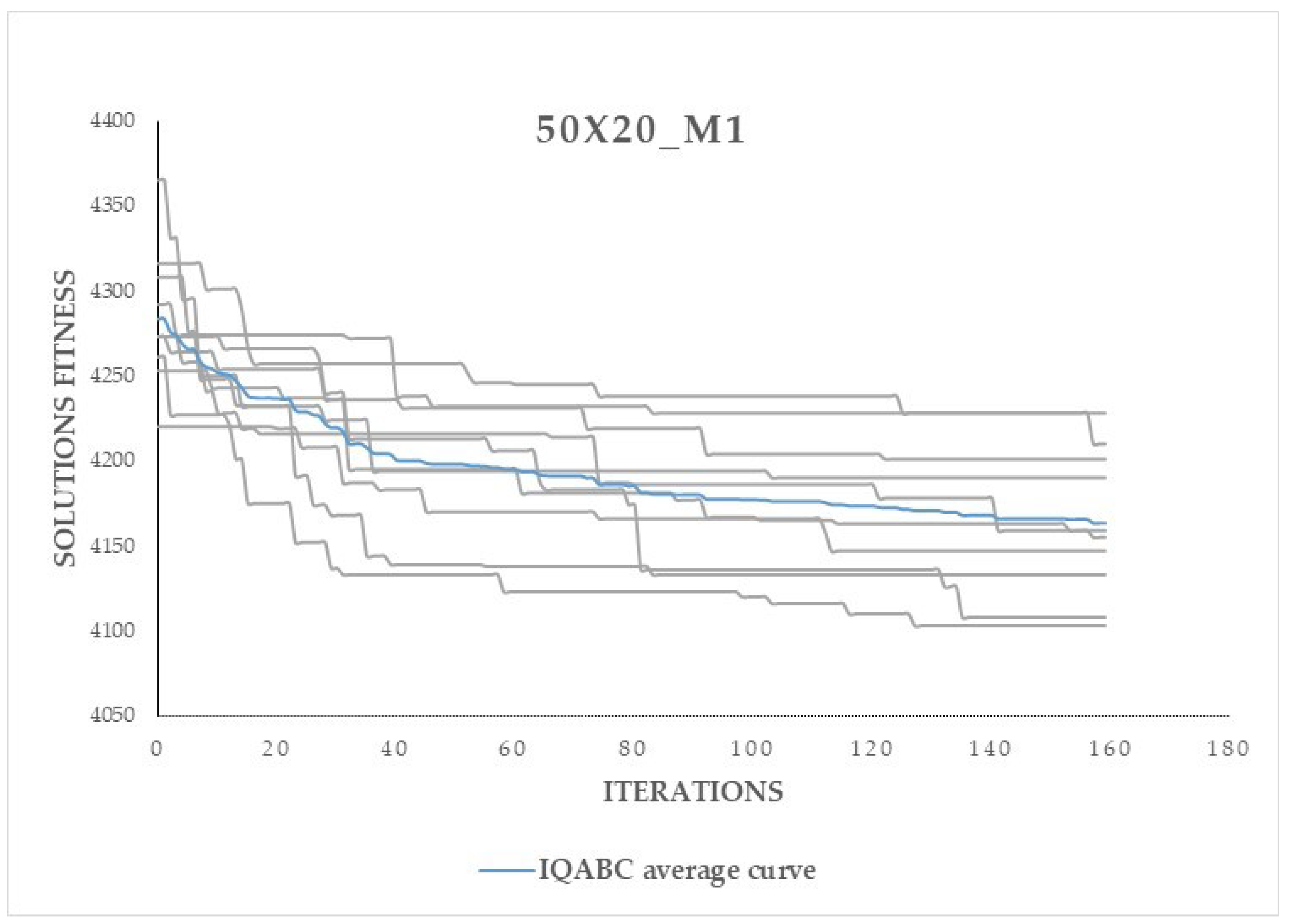
In Figure 3, Figure 4, Figure 5 and Figure 6, we also compare the convergence curves of the IQABC and ABC algorithms. We note that the ABC algorithm is more likely to become trapped in premature convergence, while the IQABC algorithm still finds better optimal solutions at a relatively more efficient rate, and the better results can be obtained at the final stage. We can conclude that the QL algorithm in the employed bees phase helps the IQABC algorithm to converge in a robust and efficient way. This conclusion is supported by the convergence curves of 10 trials on the instance 50x20_M1 as well as the average convergence curve in bold in Figure 7.

It is important to note that high ARPD values do not reflect poor solution quality since they are calculated relative to the best-known Taillard solutions, without taking into account maintenance tasks and learning/deterioration effects. Therefore, the presented ARPD deviations (for all experiments) are much higher than they would be if they were calculated with respect to a more accurate lower bound that takes into account maintenance tasks and learning/deterioration effects.

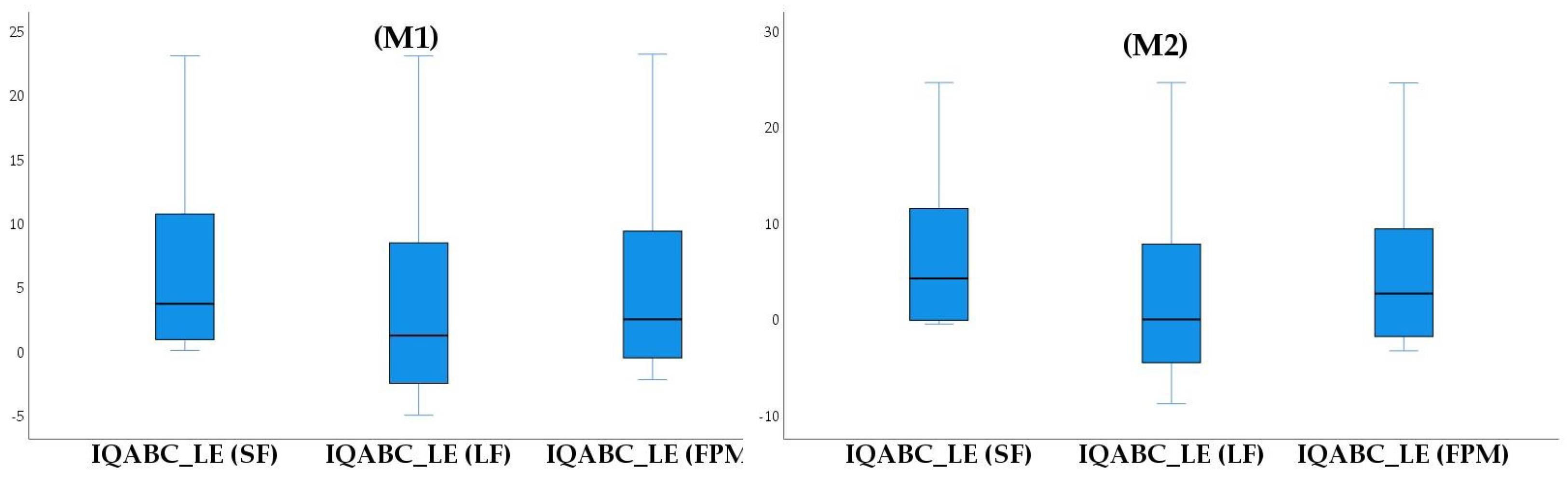
5.4. Performance Analysis of the QL-Driven ABC Algorithm with Learning Effect

The performance of the first algorithm, namely the IQABC-LE, is proven through three scenarios and 1100 executions per scenario on the designed benchmarks completed with learning indexes ($\alpha$). First, we assume a small common learning rate among maintenance operators, so we generate small learning indexes (SF) from the uniform distribution $\mathcal{U}[0;0.20]$. Then, assuming that the operators learn very quickly at the same rate, large learning indices (LF) are generated from the uniform distribution $\mathcal{U}[0.80;1]$. Finally, we assume that the learning phenomenon is random and depends on the machine characteristics, so the learning indexes are generated from the uniform distribution $\mathcal{U}[0;1]$ per machine (FPM).

The execution results are compared with the ABC learning algorithm (ABC-LE) reported in [54]. Indeed, the IQABC-LE algorithm implements a QL mechanism to guide the neighbor structure selection in the employed bees phase, instead of random selection as in ABC-LE. In addition, the IQABC-LE uses the INEH heuristic to generate one complete solution, while the ABC-LE algorithm applies the NEH heuristic [43] to generate first, the production sequence, then, the maintenance heuristic[44] to complete the solution with maintenance emplacements.

The comparison between the two algorithms is made according to the ARPD values, which are calculated on the basis of the $C_{max}$ values given in Formula (4).

The results presented in

Table 3. Performance offset from Taillard’s upper bounds of IQABC-LE and ABC-LE considering small learning indexes.

Instance	M1		M2
	ABC-LE(SF)	IQABC-LE(SF)	ABC-LE(SF)	IQABC-LE(SF)
20x5	4.47	2.79	3.35	3.33
20x10	12.81	11.36	14.44	12.27
20x20	24.76	23.24	27.20	24.88
50x5	1.87	0.27	2.24	−0.25
50x10	8.98	5.43	12.26	6.27
50x20	19.43	14.65	23.37	16.26
100x5	0.39	0.25	0.38	−0.14
100x10	3.7	2.37	4.93	2.50
100x20	12.39	10.46	14.46	11.28
200x10	0.43	0.76	0.74	−0.13
200x20	6.31	5.01	7.16	5.66
500x20	1.26	1.43	0.23	0.42
average	8.07	6.50	9.23	6.86

,

Table 4. Performance offset from Taillard’s upper bounds of IQABC-LE and ABC-LE considering large learning indexes.

Instance	M1		M2
	ABC-LE(LF)	IQABC-LE(LF)	ABC-LE(LF)	IQABC-LE(LF)
20x5	4.73	3.06	3.29	3.51
20x10	13.34	11.47	14.22	12.52
20x20	25.1	23.23	26.95	24.88
50x5	0.21	−1.06	−0.43	−2.53
50x10	6.85	3.70	8.15	2.97
50x20	16	12.35	18.69	12.39
100x5	−2.82	−3.15	−4.3	−4.94
100x10	−0.4	−1.45	−1.62	−3.60
100x20	7.71	5.83	6.52	3.75
200x10	−3.87	−4.13	-6.36	−7.05
200x20	0.7	−0.22	−1.36	−2.52
500x20	−4.39	−4.79	−8.17	−8.52
average	5.26	3.73	4.63	2.57

and

Table 5. Performance offset from Taillard’s upper bounds of IQABC-LE and ABC-LE considering random learning indexes per machine.

Instance	M1		M2
	ABC-LE(FPM)	IQABC-LE(FPM)	ABC-LE(FPM)	IQABC-LE(FPM)
20x5	4.4	2.95	3.38	3.44
20x10	13.69	11.42	14.20	12.23
20x20	25.11	23.38	27.28	24.84
50x5	0.76	−0.47	1.24	−1.48
50x10	7.63	4.51	9.86	4.39
50x20	17.66	13.44	20.96	14.34
100x5	−1.47	−1.24	−1.55	−3.02
100x10	1.84	0.47	1.52	−0.38
100x20	9.9	7.70	9.30	7.05
200x10	−1	−2.01	−2.10	−2.74
200x20	3.45	2.40	3.19	2.41
500x20	−0.52	−0.16	−2.49	−1.61
average	6.79	5.19	7.06	4.95

clearly show the superiority of the IQABC-LE algorithm over the ABC-LE algorithm. An important note comparing the results of the IQABC algorithm when considering a learning effect and no effect, is the significant difference in ARPD values, which increasingly reinforce the need to take into account real constraints when studying scheduling problems.

From Figure 8, it can be seen that the IQABC-LE algorithm with large learning indexes (LF) optimizes the $C_{max}$ very well compared to the small and random learning indexes. Consequently, it is of great importance for a workshop to improve the ability of its employees to learn.

5.5. Performance Analysis of the QL-Driven ABC Algorithm with Learning and Deteriorating Effects

In this section, the IQABC-LDE algorithm with a learning and deteriorating effect is evaluated on the designed benchmarks completed with random learning and deteriorating indexes generated from a uniform distribution $\mathcal{U}[0,1]$. The results of the 1100 executions are summarized in

Table 6. Performance offset from Taillard’s upper bounds of IQABC-LDE and ABC-LDE considering random learning and deteriorating indexes per machine.

instance	M1		M2
	ABC-LDE	IQABC-LDE	ABC-LDE	IQABC-LDE
20x5	13.04	9.64	12.45	9.24
20x10	23.66	19.31	23.02	19.05
20x20	37.3	30.82	36.17	32.10
50x5	11.30	7.96	12.09	8.59
50x10	18.49	14.09	19.32	13.85
50x20	28.54	23.09	30.06	23.17
100x5	10.84	7.85	11.45	5.62
100x10	13.29	10.41	13.32	8.87
100x20	21.41	17.43	20.32	15.55
200x10	12.86	9.56	8.91	7.18
200x20	17.69	12.92	15.01	12.08
500x20	13.04	9.84	12.45	8.71
average	18.45	14.40	17.88	13.66

and compared to those of the ABC-LDE reported in [54]. The ABC-LDE follows the same steps as the ABC-LE, with the addition of the deteriorating effect. The ARPD values reported in Table 6 are calculated on the basis of the $C_{max}$ values given in Formula (5).

Once again, the IQABC-LDE is superior to the ABC-LDE, proving the effectiveness and robustness of the QL-based neighbor selection mechanism when combined with the ABC metaheuristic. As with the learning effect, we observe a significant difference in the results obtained with the IQABC algorithm if the learning and degradation effects are not taken into account, thus emphasizing the need to integrate these effects into the study. In fact, the deteriorating effect, as opposed to the learning effect, extends processing times. It is therefore important for manufacturers to implement an efficient maintenance strategy to prevent machines from deteriorating and additional delays.

6. Conclusions

We addressed the makespan PFSP with flexible maintenance under learning and deteriorating effects. The maintenance operations are inserted to prevent machine failures with an intelligent PHM-based policy. In addition, the learning effect on the maintenance duration is considered and modeled by a decreasing position-dependent function. On the other hand, the deteriorating effect is assumed to extend the job processing times over time. For the resolution, the well-known ABC algorithm, which has been successfully applied to solve the PFSP without learning and deterioration effects, is adapted to the problem with flexible maintenance, learning, and deteriorating effects in order to find a faster and near-optimal or optimal solution to the problem. To improve the local search in the ABC-employed bees phase, a QL algorithm, considered a common potential tool of the RL mechanism, is carefully integrated into the ABC metaheuristic. Furthermore, a newly designed heuristic, the INEH, is applied to enrich the search space with a high-quality complete solution. The adapted ABC algorithm with the new strategies is used to first solve the integrated PFSP with a learning effect (IQABC-LE) and then also with a deteriorating effect (IQABC-LDE). We conducted a comprehensive experimental study to evaluate the IQABC algorithm without considering the learning and deteriorating effects, the IQABC-LE and IQABC-LDE algorithms. The objective of evaluating these three algorithms is, on the one hand, to justify the significance of our study when we have considered the learning and deteriorating effects, and on the other hand, to prove the effectiveness and robustness of our newly proposed algorithms. For the latter purpose, the experimental results are compared with those of two existing and competitive metaheuristics in the literature: ABC and VNS. The computational results and comparisons demonstrate that the new strategies of the IQABC approach really improve its search performance and IQABC is a competitive approach for the considered problem. Moreover, the need to consider learning and deterioration effects for a more realistic and accurate study is also demonstrated and emphasized. For future work, we propose to integrate more realistic constraints such as the forgetting effect and human resource constraints in the study of the PFSP. We also expect to apply other recently introduced bio-inspired metaheuristics, such as BBO and GWO, to solve the studied scheduling problem, and compare the results with the ABC algorithm.