Variable Scale Pruning for Transformer Model Compression in End-to-End Speech Recognition

Abstract

Transformer models are being increasingly used in end-to-end speech recognition systems for their performance. However, their substantial size poses challenges for deploying them in real-world applications. These models heavily rely on attention and feedforward layers, with the latter containing a vast number of parameters that significantly contribute to the model’s memory footprint. Consequently, it becomes pertinent to consider pruning these layers to reduce the model’s size. In this article, our primary focus is on the feedforward layers. We conduct a comprehensive analysis of their parameter count and distribution. Specifically, we examine the weight distribution within each layer and observe how the weight values progress across the transformer model’s blocks. Our findings demonstrate a correlation between the depth of the feedforward layers and the magnitude of their weights. Consequently, layers with higher weight values require less pruning. Building upon this insight, we propose a novel pruning algorithm based on variable rates. This approach sets the pruning rate according to the significance and location of each feedforward layer within the network. To evaluate our new pruning method, we conduct experiments on various datasets. The results reveal its superiority over conventional pruning techniques, such as local pruning and global pruning.

1. Introduction

Transformer architecture has gained significant attention recently and has emerged as the state-of-the-art approach in various sequence-to-sequence tasks. These tasks encompass a wide range of applications, such as natural language processing [1], image retrieval [2], emotion detection [3], and speech recognition [4]. In the domain of speech recognition, transformer architecture has enabled the development of end-to-end automatic speech recognition (ASR) systems. Indeed, the advantage of an end-to-end ASR system is that it eliminates the requirement for multiple modules, such as the lexicon, acoustic models, and linguistic models, found in conventional hidden Markov models [5] or hybrid models that combine neural networks with hidden Markov models [6]. Instead, in end-to-end systems, all the necessary acoustic and linguistic knowledge is seamlessly integrated within a single neural network. This integration simplifies the ASR process by consolidating all relevant information into a unified framework. However, the transformer models used in various applications, including automatic speech recognition, tend to be excessively large and over-parameterized, as highlighted in [7,8,9].

The complexity of these models has consequences on the memory requirements and the computational cost. These issues can be addressed by studying compression methods that could have the following outcomes [10]:

-

Memory Usage Reduction: Compressing transformer models helps mitigate excessive memory requirements, allowing for more efficient utilization of resources.

-

Prediction Latency and Energy Consumption: By compressing the models, prediction latency is reduced, resulting in faster and more energy-efficient computations.

-

Inference on Resource-Constrained Devices: Compressed transformer models enable their deployment on devices with limited hardware resources, such as mobile devices, making ASR systems more accessible and efficient.

-

Ease of Learning, Fine-Tuning, and Distributed Training: Compressed models are easier to train, fine-tune, and distribute, facilitating their adoption in various settings and scenarios.

-

Ease of Deployment and Updating: Compressed transformer models offer advantages in terms of deployment and updating processes, enabling seamless integration into production systems.

The literature on model compression encompasses a wide range of techniques aimed at addressing the challenges posed by large and over-parameterized models. For instance, Qi et al. [11] established a theoretical understanding of the architecture of deep neural networks, exploring their representation and generalization capabilities for speech processing, which, in turn, affect the empirical performance of the pruned ASR model. Furthermore, in their work, Qi et al. [12] proposed an alternative model compression technique based on the tensor-train network to reduce the complexity of the ASR model.

In general, model compression techniques involve quantization [13], pruning [14], knowledge distillation [15], matrix decomposition [16], and parameter sharing [17]. In the field of automatic speech recognition (ASR), pruning has been successfully employed in various model architectures, such as the multilayer perceptron (MLP), as studied in [18]; long short-term memory (LSTM) networks, as explored in [19]; convolutional neural networks (CNN), as described in [20]; and their combinations, as investigated in [21]. Regarding transformer-based ASR systems, research has focused on quantization [22], parameter sharing [7], weight magnitude pruning [23], and, recently, on knowledge distillation [24].

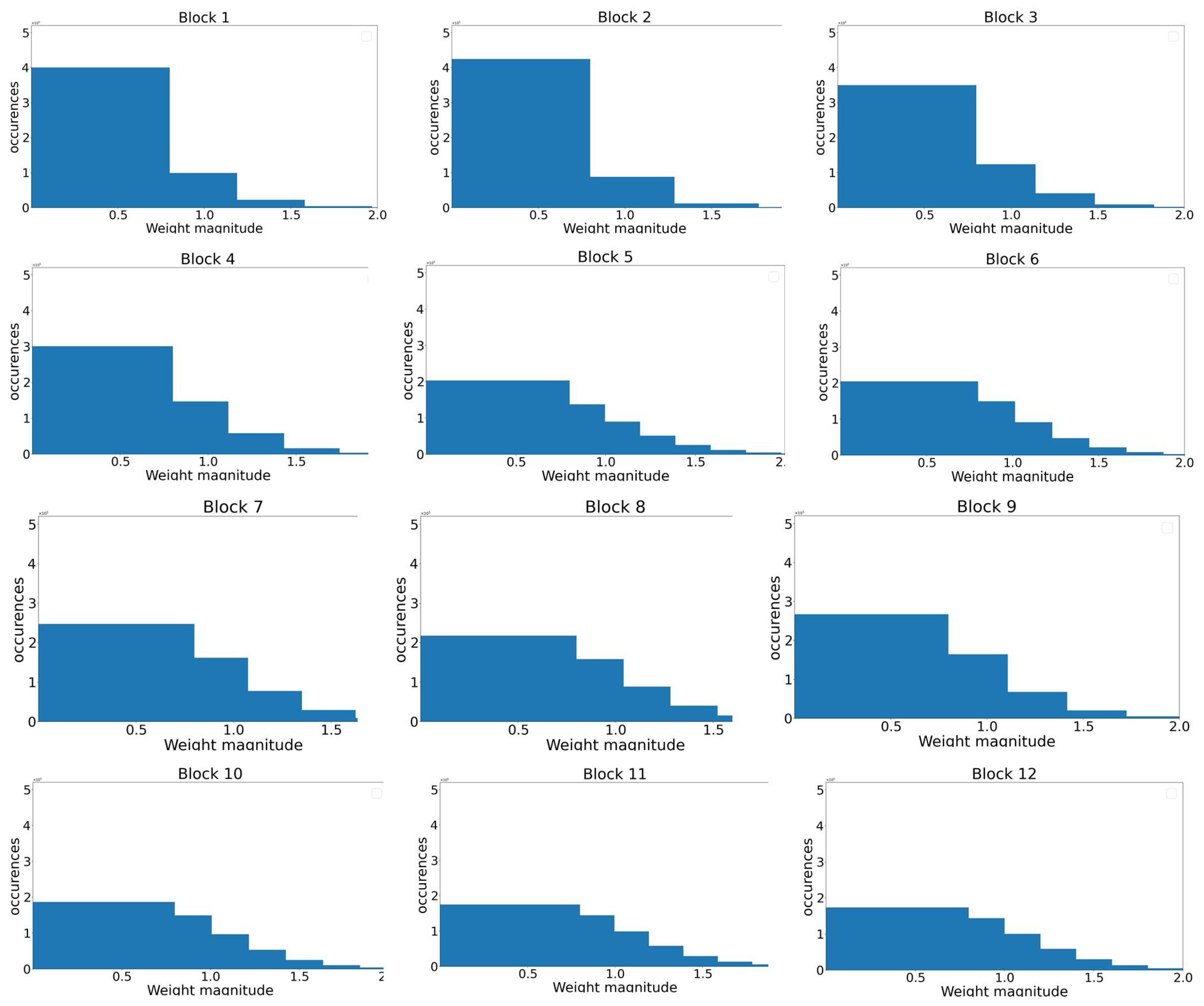
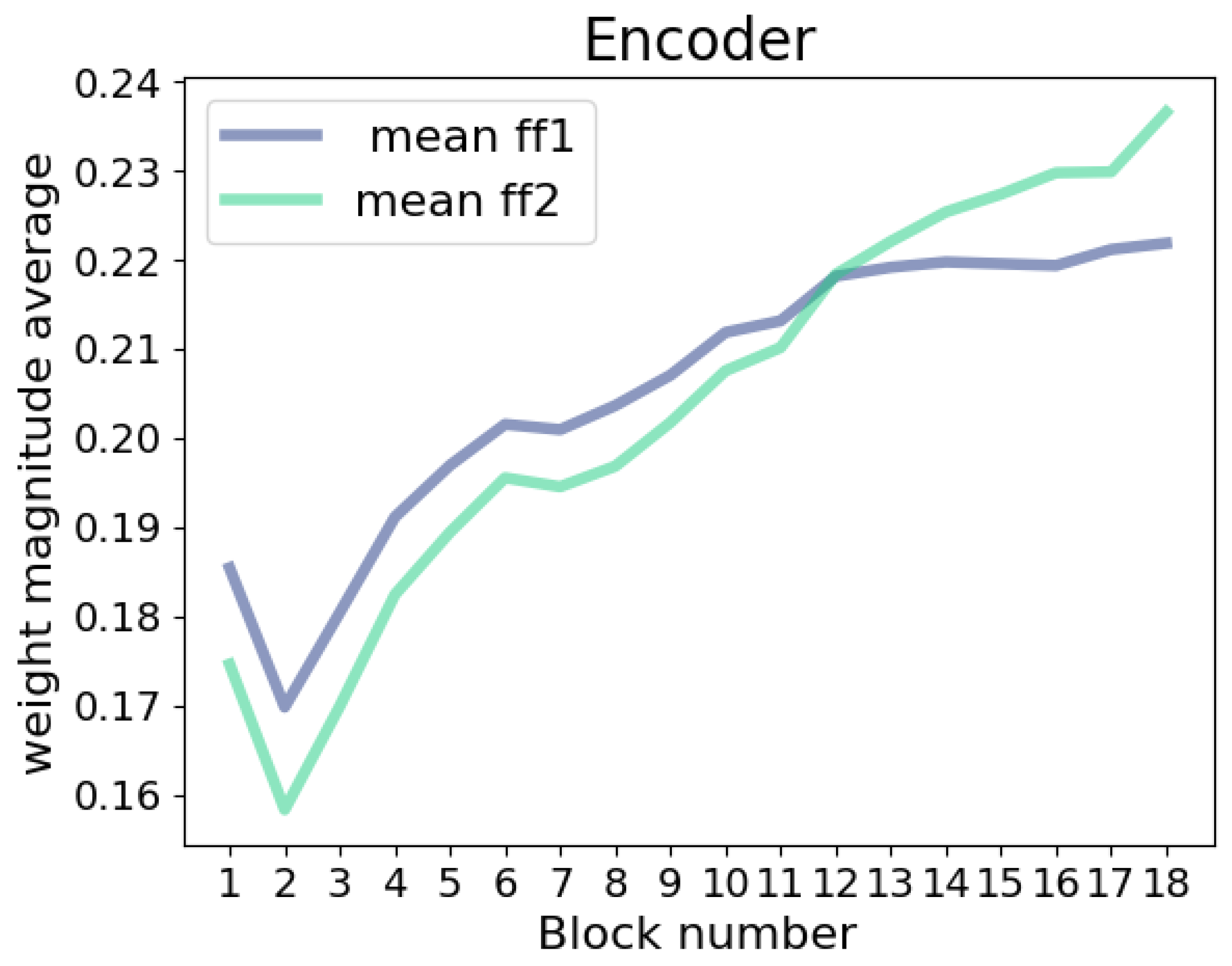
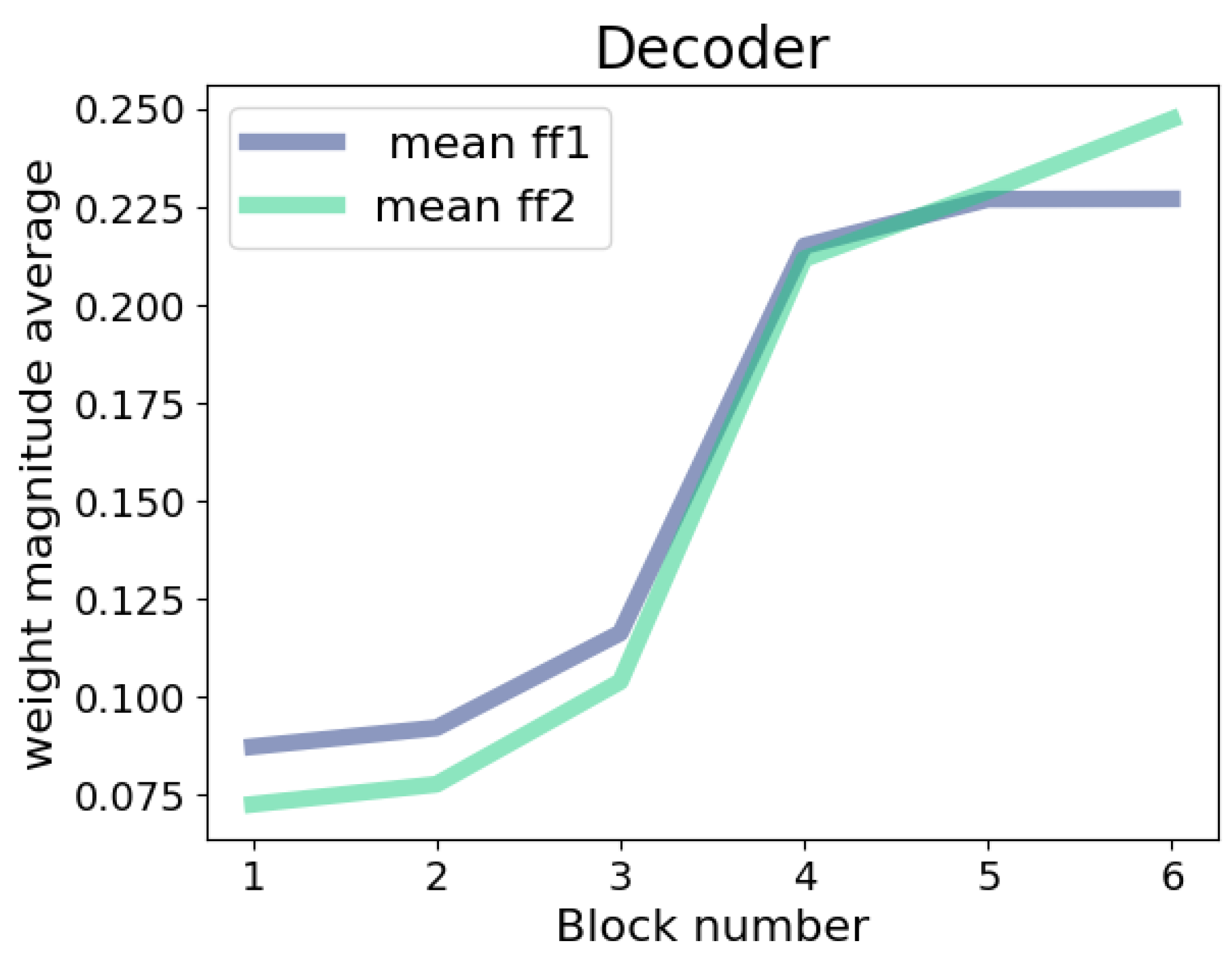
In particular, in [23], we conducted a comprehensive analysis of ASR transformer models across multiple languages. Our findings revealed that the feedforward layers, in comparison to other layers in the model, have the highest parameter count, occupying a substantial portion of the model’s overall size. Furthermore, as these layers undergo global pruning, their Sparsity progressively decreases. The current paper is an extension of this work. Consequently, the focus of the research was directed towards pruning the feedforward layers. To achieve this, the weights of the feedforward layers were examined within each block and between encoder blocks and decoder blocks. This analysis uncovered a progressive distribution of weights in the feedforward layers, with deeper layers having higher weight values. Based on these insights, the primary contribution of the research was the proposal of a pruning technique that takes into account the layer positioning and gradually reduces the weights of the feedforward layers.

The structure of this paper is as follows: Section 2 provides a comprehensive review of the relevant literature and prior work in the field. Section 3 offers a detailed description of the ASR transformer model under investigation. Subsequently, Section 4 introduces the proposed variable scale pruning method. The experimental setup and results are presented in Section 5. Finally, Section 6 discusses the obtained results and provides the key conclusions derived from this study.

2. Related Work

Model pruning techniques refer to a range of methods employed to decrease the size of models while maintaining performance levels within an acceptable range [10]. These techniques focus on removing redundant parameters or structures from neural networks, resulting in a reduced memory footprint and computational demands. By doing so, model pruning enhances generalization, reduces the dependency on a large number of training examples, and accelerates the speed of learning and/or classification processes [14].

2.1. Pruning Structure

Pruning methods can be broadly categorized into two main groups [10]:

• Unstructured pruning [2], which is a pruning technique that involves removing individual weights from a weight matrix. When a weight value is replaced with zero, it effectively prunes a connection. This type of pruning is commonly referred to as sparse pruning [23], as it results in sparse matrices (as shown on Figure 1b).
• Structured pruning [25] is a pruning technique that specifically targets the removal of entire blocks of weights, rather than individual weights, within a neural network. This approach enables pruning at a higher level of granularity, allowing for the elimination of larger structural components. For instance, in fully connected layers [26], it is possible to zero out blocks of connections (refer to Figure 1d), or even entire rows or columns of a weight matrix (as shown on Figure 1c), resulting in the removal of entire neurons. Similarly, in convolutional neural networks (CNNs), filters or channels can be removed, and in transformer models [27,28], even attention heads can be pruned.

Pruning can be incorporated into the training process as an additional step between training epochs (iterative pruning), applied all at once after the model training is complete (one-shot pruning) [13], or applied between fine-tuning steps [25]. The importance of the weights can be determined by their magnitude [29], their gradients [30], or a custom measurement [31].

Our focus lies on unstructured pruning, specifically targeting the removal of connections. This approach centers on pruning the smallest independent elements of the model, which allows for pruning in large quantities without significant impacts on performance.

2.2. Sparse Matrix

Nonetheless, unstructured pruning comes with certain limitations. A significant drawback is the Sparsity that arises within the pruned model. This Sparsity manifests as numerous parameters with zero values, leading to irregular memory access patterns that may not be efficiently optimized by conventional hardware architectures. To address this concern, specific approaches can be adopted, such as utilizing sparse matrix representations [32] or employing hardware accelerators [33] designed explicitly for sparse computations.

When dealing with sparse matrices [34], significant reductions in memory requirements can be achieved by storing only the non-zero entries. There are several ways to represent sparse matrices, such as the Coordinate List (COO), the Compressed Sparse Row (CSR), and the Compressed Sparse Column (CSC) [32]. Regarding sparse matrix hardware accelerators, they often employ specialized architectures and algorithms that leverage the Sparsity of the matrix to minimize memory usage and optimize computational operations. They can provide efficient storage and processing of sparse matrices, allowing for faster matrix–vector multiplications, matrix factorization, and other operations commonly used in scientific computing, machine learning, and graph analytics. They play a crucial role in accelerating computations involving sparse matrices, enabling faster and more efficient processing of data with a reduced memory footprint and improved performance.

The objective of the FVLLMONTI project (fvllmonti.eu), of which this research work is a part, is to create 3D stacked hardware layers for neural networks. The goal is to achieve highly efficient speech recognition and machine translation through meticulous hardware/software co-optimization. To this end, a hardware accelerator [33] utilizing a sparse matrix representation will be utilized in this pursuit.

2.3. Pruning Schemes

Global and local pruning techniques are two common approaches used in model compression by pruning [25,35].

• Global pruning involves pruning a fixed percentage of weights across the entire model [36]. It is a systematic approach that identifies and removes the least important weights. Typically, a threshold is set, and weights below this threshold are pruned. Global pruning aims to reduce the overall size of the model by eliminating a portion of the weights (see Figure 2). However, it may not take into account the specific importance of weights in different parts of the model.
• Layer-wise pruning, also known as local pruning, specifically targets individual layers within a model for pruning. This technique, also referred to as class-uniform pruning [29], entails removing a fixed percentage of parameters from each layer, as shown on Figure 2.

The study conducted in [2] applies class distribution pruning, where the pruning threshold for each layer is determined by multiplying a quality parameter with the standard deviation of the layer’s weights. This approach is compared with global and local pruning methods [36]. The results demonstrate that global pruning yields the best performance among the three techniques.

3. ASR Transformer

The transformer model [1] is a sequence-to-sequence architecture designed to map an input sequence $(x_1,x_2,\dots ,x_T)$ to an output sequence $(y_1,y_2,\dots ,y_L)$. Its structure consists of two main components: the encoder and the decoder. The encoder takes the input sequence and transforms it into an intermediate sequence of encoded features $(h_1,h_2,\dots ,h_N)$. On the other hand, the decoder generates predictions for each character $y_l$ based on the encoded features $(h_1,h_2,\dots ,h_N)$ and the previously decoded characters $(y_1,y_2,\dots ,y_{l-1})$. Both the encoder and the decoder comprise a stack of attention and feedforward network blocks, allowing the model to capture contextual dependencies and make accurate predictions.

3.1. Model Architecture

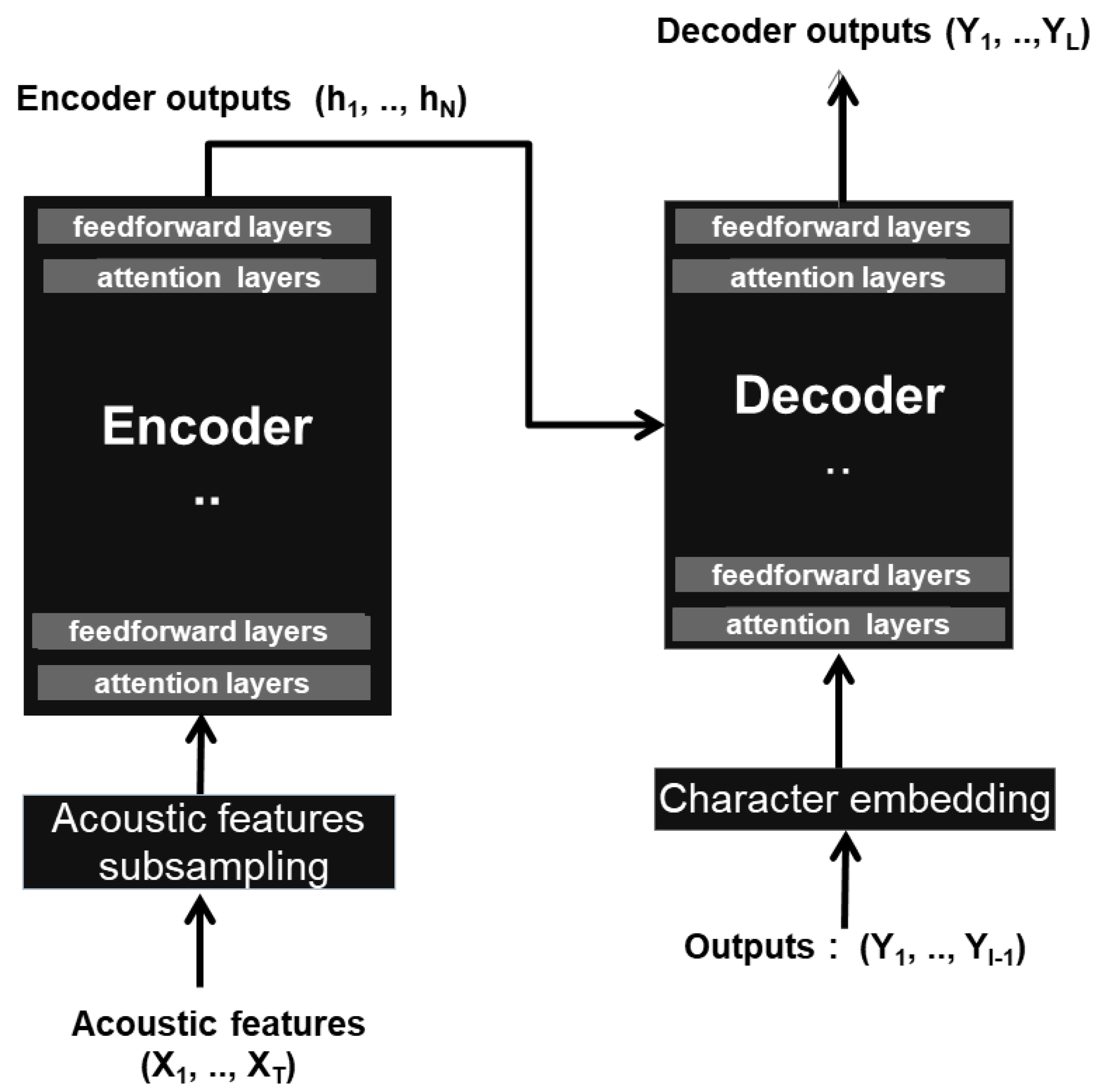
Our ASR transformer model adopts the architecture described in [37]. Prior to entering the encoder, the input acoustic features undergo subsampling via two convolution layers. The encoder and decoder modules consist of multi-head attention (MHA) and feedforward (FF) layers. Each layer is accompanied by a residual connection and normalization. Figure 3 provides a simplified illustration of the ASR transformer model’s structure.

The layers of the encoder refine the representation of the input sequence with a suite of multi-head, self-attention, and linear transformations. The self-attention operation allows frames to gather context from all timesteps and build an informative sequence at a high level [37]. Specifically, the inputs of each layer are projected into queries Q, keys K, and values V with $Q\in {\mathbb{R}}^{t_q\ast d_q}$, $K\in {\mathbb{R}}^{t_k\ast d_k}$, and $V\in {\mathbb{R}}^{t_v\ast d_v}$. $t\ast$ are the elements numbers in different inputs and $d\ast$ are the corresponding element dimensions. Usually, these are $t_k=t_v$ and $d_q=d_k$.

Scaled Dot-Product Attention [1] is then computed as:

$$Attention(Q,K,V)=softmax\left(\frac{Q{K}^T}{\sqrt{d_k}}\right)V$$

(1)

The MHA is applied to take advantage of the different representations that are simultaneously present. The multi-head attention is obtained by performing this calculation h times. h is the number of heads.

$$MultiHead(Q,K,V)=Concat(hea{d}_1,...,hea{d}_h)W_0$$

(2)

where

$$hea{d}_i=Attention(Q{W}_i^Q,K{W}_i^K,V{W}_i^V)$$

(3)

The projection matrices are $W_i^Q\in {\mathbb{R}}^{d_{model}\ast d_q}$, $W_i^K\in {\mathbb{R}}^{d_{model}\ast d_k}$, $W_i^V\in {\mathbb{R}}^{d_{model}\ast d_v}$, and $W^0\in {\mathbb{R}}^{h\ast d_v\ast d_{model}}$. In this work, $d_k=d_q=d_v=d_{model}/h$.

The outputs of multi-head attention go through a two-layer position-wise feedforward network (FFN) with hidden size $d_{ff}$ [1].

$$FFN\left(x\right)=W_{2}ReLU(W_{1}x+b_1)+b_2$$

(4)

$b_1\in {\mathbb{R}}^{d_{ff}}$ and $b_2\in {\mathbb{R}}^{d_{model}}$ are the biases. The weight matrices are $W_1\in {\mathbb{R}}^{d_{model}\ast d_{ff}}$ and $W_2\in {\mathbb{R}}^{d_{ff}\ast d_{model}}$.

3.2. Model Development

For the development of end-to-end transformer models, we used the Libri-trans [38] and VoxforgeIT [39] datasets in conjunction with the Espnet toolkit [4].

Libri-trans is a subset of the LibriSpeech database, which was created as part of the Librivox project (librivox.org) [40]. It contains 236 h of annotated English utterances from audiobooks. VoxforgeIT, on the other hand, is an Italian dataset developed within the Voxforge project (voxforge.org) and provides 20 h of audiobooks. Both datasets are divided into three sets: a training set, a development set, and a test set. For the Libri-trans dataset, 231 h are used for model training, while 2 h and 3.45 h are allocated for the development and evaluation sets, respectively. In the case of VoxforgeIT, 80% of the data are used for training, and the remaining data are evenly split between the development and test sets. To augment the data, we applied speed perturbation [41] with ratios of 0.9, 1.0, and 1.1. This technique effectively multiplies the quantity of data by three, providing additional variations for training.

Espnet is an open source toolkit that integrates Kaldi [42] tools for data processing and parameter extraction, along with PyTorch (pytorch.org) modules for model estimation. For the input features, we computed 80 filter bank coefficients, which were then normalized based on the mean and variance. Filter bank (F-bank) parameters enable the extraction of relevant information from speech signals in the frequency domain. By capturing the spectral content of speech, they provide a representation that is more suitable for various speech processing tasks including speech recognition.

As for the representation of transcripts, we used subword units. Specifically, the VoxforgeIT system utilizes character-level representation, while the Libri-trans system employs byte-pair coding subwords. For the training stage, we ran stochastic gradient descent (SGD) over the training set with the Adam update rule [43] using square root learning rate scheduling [1] (25,000 warmup steps and 64 minibatch sizes). The architecture of the developed models is illustrated in

Table 1. Architecture of the transformer models: number of encoder and decoder blocks, dimension of feedforward layers, dimension of attention layers, and number of attention heads.

	Encoder Blocks	Decoder Blocks	Feedforward Dim	Attention Dim	Heads Number
Libri-trans	12	6	1024	256	4
VoxforgeIT	18	6	2048	256	4

. The Libri-trans model consists of 27.92 million parameters, while the VoxforgeIT model has 35.07 million parameters. This corresponds to approximately 107 and 134 megabytes of memory, respectively.

The performance of these models in Automatic Speech Recognition (ASR) is as follows: In the case of Libri-trans, the Word Error Rate (WER) achieved was 6.6% on the test set and 6.3% on the development set. These results surpass the current state-of-the-art performance of 15.1% reported in [44] on the test set. As for VoxforgeIT, the Character Error Rate (CER) obtained was 9.3% on the test set and 10.3% on the development set. These results also outperform the state-of-the-art performance of 9.6% documented in [45] on the test set.

4. Adaptive Pruning

Within this section, we will introduce our suggested technique for pruning the ASR transformer model.

4.1. Model Sizing

The ASR transformer model comprises three main components: the embedding, the encoder, and the decoder. The acoustic embedding involves two convolution layers responsible for subsampling the acoustic features. The encoder and decoder consist of multiple blocks of attention layers (ATs) and feedforward layers (FFs). Each layer is accompanied by a residual connection and normalization. Figure 4 illustrates the distribution of the encoder and decoder parameters.

According to Figure 4, the feedforward layers contain the majority of parameters, accounting for over 60% of the total model size. Consequently, our focus in the subsequent discussion will be primarily on these feedforward layers.

4.2. Feedforward Layers’ Behaviour

In every encoder and decoder block, there exist two feedforward (FF) layers, denoted as FF1 and FF2. Our focus is on examining the weight distribution of these FF1 and FF2 layers. To accomplish this, we visualize the histograms displaying the weight magnitudes of the FF1 encoder layers in Figure 5. Upon observation, we noticed a trend where the weight magnitudes are relatively low in the initial layers, progressively increasing as the layers become deeper.

Figure 6 and Figure 7 provide evidence to support this observation, as they demonstrate the progression of the average weight magnitude across the FF1 and FF2 layers in both the encoder and decoder.

4.3. Feedforward Layers’ Adaptive Pruning

The variable scale pruning method we propose focuses on pruning the early feedforward layers to a greater extent compared with the deeper layers. This approach involves utilizing a decreasing pruning rate (see Figure 8). Assuming that the pruning rate of the feedforward layers follows an arithmetic sequence, we define two sequences: U with parameter $\alpha$ representing the pruning rate of the encoder layers, and V with parameter $\beta$ representing the pruning rate of the decoder layers. When considering two consecutive layers n and $n+1$, with $U_n$ denoting the pruning rate of the current layer and $U_{n+1}$ representing the pruning rate of the next layer, the following relationship holds:

$$U_{n+1}=U_n-\alpha$$

(5)

If n and $n+1$ are decoder layers, then:

$$V_{n+1}=V_n-\beta$$

(6)

where $\alpha$ and $\beta$ are positive numbers. For the first layers of the encoder and decoder, the initial pruning rates $U_0$ and $V_0$ are set empirically.

Figure 8. Adaptive pruning: layer n is pruned with a pruning rate $U_n$, while layer $n+1$ is pruned with a lower pruning rate $U_{n+1}$, where $U_n>U_{n+1}$.

Figure 8. Adaptive pruning: layer n is pruned with a pruning rate $U_n$, while layer $n+1$ is pruned with a lower pruning rate $U_{n+1}$, where $U_n>U_{n+1}$.

5. Experiments and Results

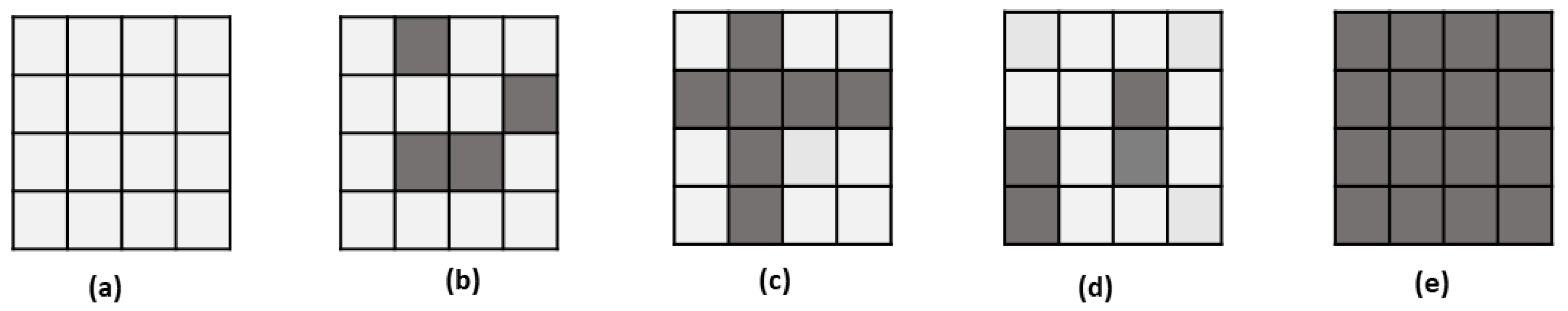
The evaluation of various pruning techniques, including global, local, and variable scale (i.e., adaptive), was performed using the transformer models described in Section 3.2. Unstructured pruning with the L1 norm were employed to prune connections. Individual weights were set to zero according to their magnitude. The adaptive pruning parameters for the Libri-trans and VoxforgeIT datasets were determined by utilizing the development data. Subsequently, the evaluation was conducted using the test data.

5.1. Baseline Systems

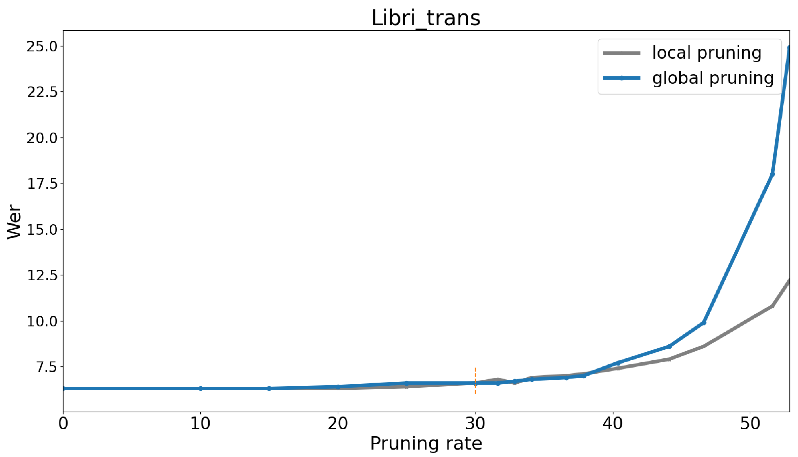
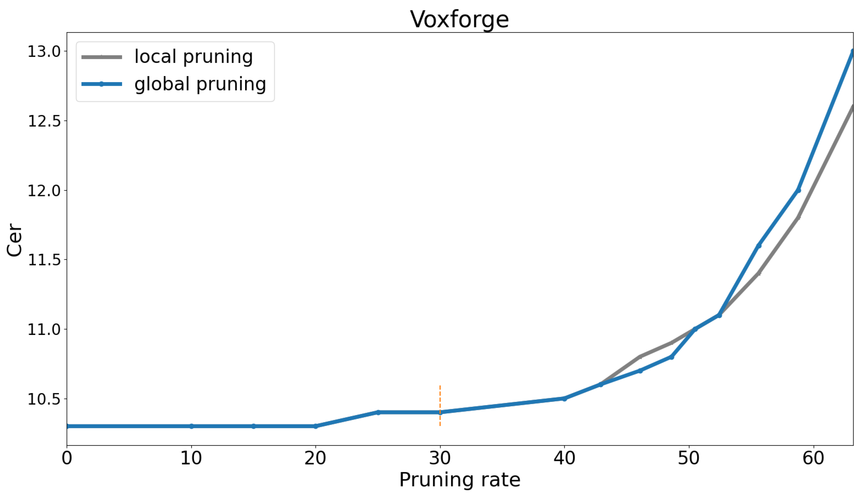
For the purpose of conducting a comparative analysis, we conducted preliminary experiments on both global and local pruning techniques utilizing the test sets from the Libri-trans and VoxforgeIT datasets. The outcomes of these experiments are illustrated on Figure 9 and Figure 10.

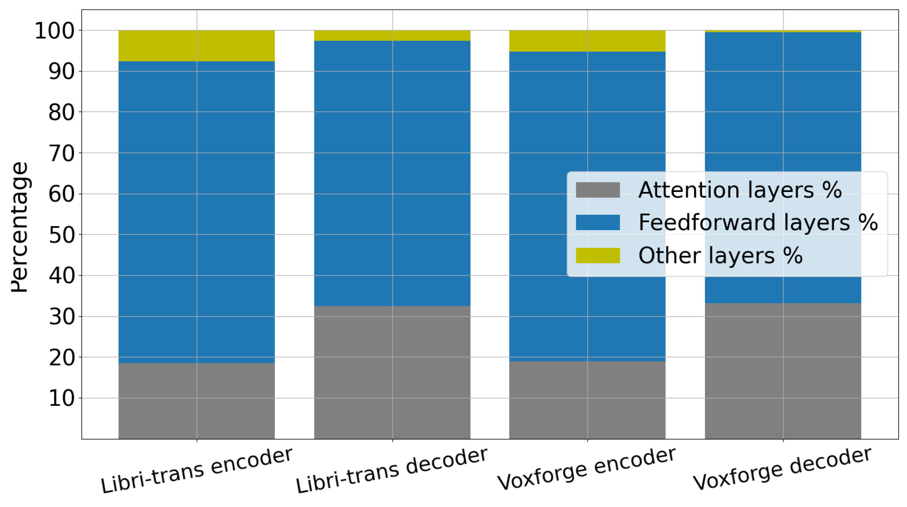
An observation we made is that when the pruning rate is 30%, there is a slight increase in the error rate of approximately 4.7% relative for Libri-trans and 2.1% for VoxforgeIT. Additionally, it is worth noting that the attention layers contribute significantly to the model size, as indicated on Figure 4. As a result, we will at least fix the attention layer pruning rate at 30% and focus on varying the pruning rate of the feedforward layers fin the subsequent analysis.

5.2. Pruning Settings

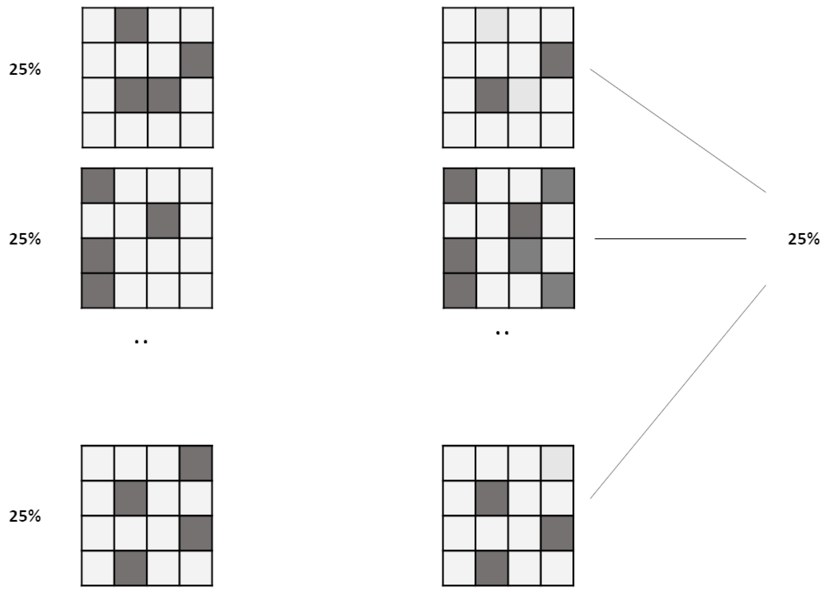
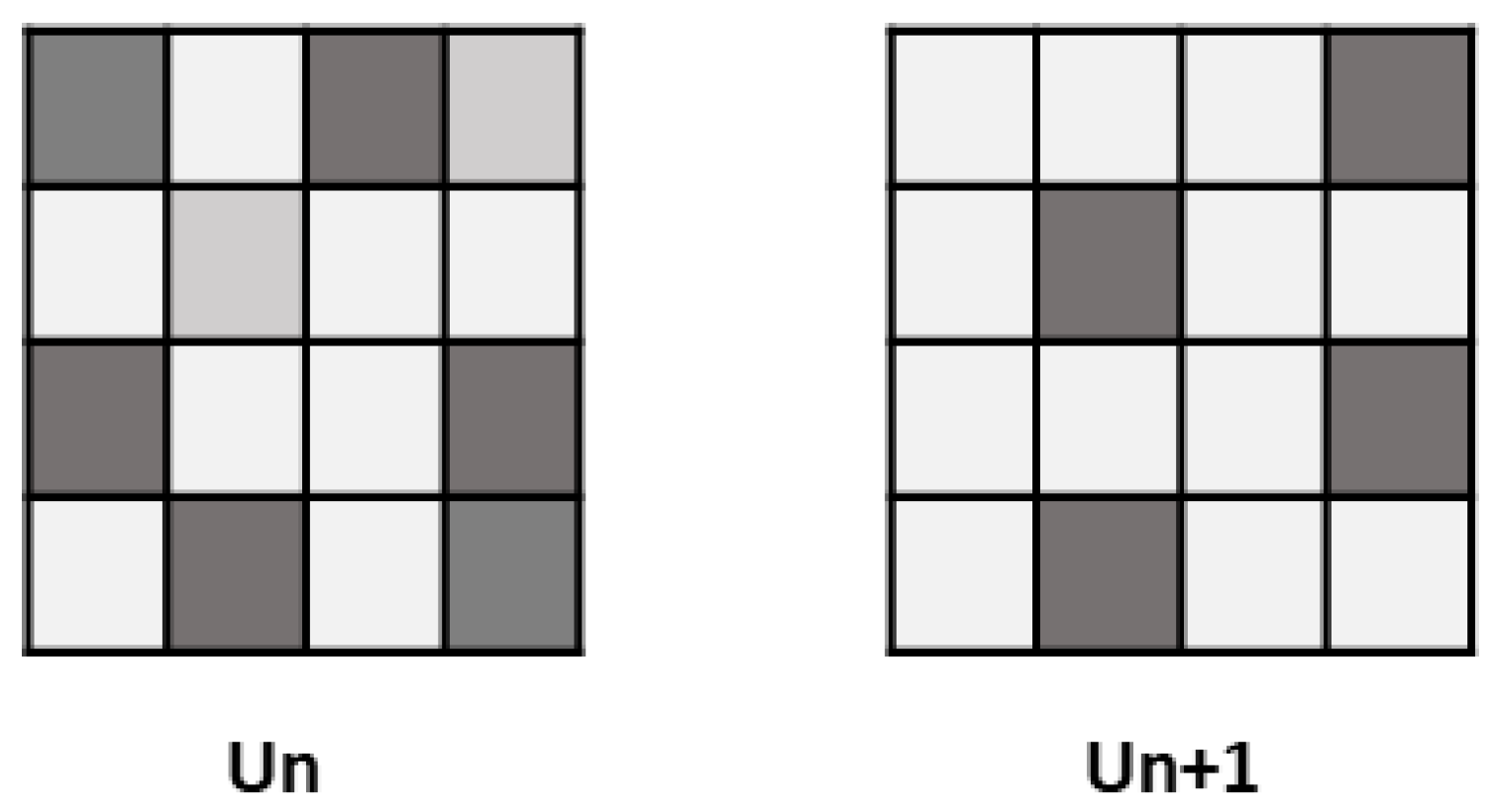
The adaptive pruning technique was applied in a single step to the feedforward and to the attention layers after the model was trained. The encoder and decoder pruning rates are represented by the arithmetic sequences U and V. To fix the initial pruning amounts $U_0$ and $V_0$ and the differences $\alpha$ and $\beta$, adaptive pruning was applied to the development data as follows:

• fix $\alpha$ and $\beta$;
• for each pair ($U_0$, $V_0$)—

  (a)

  use Formulas (5) and (6) to prune the feedforward layers;

  (b)

  evaluate the system using the pruned model and the development dataset;

  (c)

  note the error rate and the Sparsity.

The algorithm was executed three times on each dataset, with different pruning rates applied to the attention layers. Specifically, for the Libri-trans dataset, the pruning rates used were 30%, 35%, and 40%. For the VoxforgeIT dataset, the pruning rates employed were 35%, 40%, and 45%. $\alpha$ and $\beta$ were chosen empirically. For example, for a pruning rate of 30% and $\alpha$ = 0.01, the first encoder layer is pruned with the coefficient $U_0$ = 0.3; the second is pruned with $U_1$ = $U_0-\alpha$ = 0.3 − 0.01 = 0.29. Thus, for a 12th encoder block, the pruning rate of the last layer is $U_{12}$ = 0.19 (i.e., a pruning rate of 19%).

The results of the adaptive pruning technique applied to development data are reported in Appendix A. They are illustrated by

Table A1. Adaptive pruning of the Libri-trans model: WER and Sparsity. The overall pruning rate (i.e., Sparsity) of the model is derived from the values of the pairs ($U_0$, $V_0$). The fixed parameters are: attention layer pruning rate = 30% and $\alpha =\beta =0.01$.

		${\mathit{U}}_0$ (%)
${\mathit{V}}_{\mathbf{0}}$ (%)			30	35	40	45	50	55	60	65
30	WER		6.5	6.6	6.6	6.7	6.8	6.9	7.1	7.1
	Sparsity		26.62	29.12	31.62	34.12	36.62	39.12	41.62	44.12
35	WER		6.5	6.5	6.6	6.7	7.0	7.2	7.7	8.4
	Sparsity		27.87	30.37	32.87	35.37	37.87	40.37	42.87	45.37
40	WER		6.6	6.5	6.6	6.7	7.0	7.3	7.8	8.5
	Sparsity		29.12	31.62	34.12	36.62	39.12	41.62	44.12	46.62
45	WER		6.6	6.6	6.7	6.8	7.1	7.3	7.8	8.6
	Sparsity		30.37	32.87	35.37	37.87	40.37	42.87	45.97	47.87
50	WER		6.7	6.6	6.8	6.7	7.2	7.4	7.9	8.6
	Sparsity		31.62	34.12	36.62	39.12	41.62	44.12	46.62	49.12
55	WER		6.8	6.7	6.9	6.9	7.2	7.5	8.2	8.7
	Sparsity		32.87	35.37	37.87	40.37	42.87	45.37	47.87	50.37
60	WER		6.9	6.9	7.1	7.1	7.4	7.7	8.2	8.9
	Sparsity		34.12	36.62	39.12	41.62	44.12	46.62	49.12	51.62
65	WER		7.1	7.1	7.1	7.4	7.6	7.9	8.6	9.2
	Sparsity		35.37	37.87	40.37	42.87	45.37	47.87	50.37	52.87

,

Table A2. Adaptive pruning of the Libri-trans model: WER and Sparsity. The overall pruning rate (i.e., Sparsity) of the model is derived from the values of the pairs ($U_0$, $V_0$). The fixed parameters are: attention layer pruning rate = 35% and $\alpha =\beta =0.01$.

		${\mathit{U}}_0$ (%)
${\mathit{V}}_{\mathbf{0}}$ (%)			30	35	40	45	50	55	60	65	70	75
30	WER		6.6	6.6	6.6	6.7	6.9	7.2	7.7	8.3	9.5	11.6
	Sparsity		27.87	30.37	32.87	35.37	37.87	40.37	42.87	45.37	47.87	50.37
35	WER		6.7	6.6	6.7	6.8	7.0	7.2	7.8	8.4	9.6	11.8
	Sparsity		29.12	31.62	34.12	36.62	39.12	41.62	44.12	46.62	49.12	51.62
40	WER		6.7	6.6	6.7	6.8	7.1	7.3	7.8	8.5	9.7	11.9
	Sparsity		30.37	32.87	35.37	37.87	40.37	42.87	45.37	47.87	50.37	52.87
45	WER		6.7	6.6	6.8	6.9	7.3	7.3	7.9	8.5	9.6	12.1
	Sparsity		31.62	34.12	36.62	39.12	41.62	44.12	46.62	49.12	51.62	54.12
50	WER		6.8	6.7	6.9	6.9	7.3	7.4	8.1	8.6	9.7	12.0
	Sparsity		32.87	38.37	37.87	40.37	42.87	45.37	47.87	50.37	52.87	55.37
55	WER		6.9	6.8	7.0	7.0	7.4	7.6	8.3	8.8	9.9	12.2
	Sparsity		34.12	36.62	39.12	41.62	44.12	46.62	49.12	51.62	54.12	56.62
60	WER		7.0	7.0	7.1	7.3	7.5	7.8	8.4	9.0	10.1	12.6
	Sparsity		35.37	37.87	40.37	42.87	45.37	47.87	50.37	52.87	55.37	57.87
65	WER		7.1	7.1	7.2	7.3	7.7	8.0	8.5	9.3	10.4	13.3
	Sparsity		36.62	39.12	41.62	44.12	46.62	49.12	51.62	54.12	56.62	59.12
70	WER		7.4	7.3	7.4	7.6	8.0	8.2	8.8	9.6	10.9	13.6
	Sparsity		37.87	40.37	42.87	45.37	47.87	50.37	52.87	55.37	57.87	60.37

,

Table A3. Adaptive pruning of the Libri-trans model results: WER and Sparsity. The overall pruning rate (i.e., Sparsity) of the model is derived from the values of the pairs ($U_0$, $V_0$). The fixed parameters are: attention layer pruning rate = 40% and $\alpha =\beta =0.01$.

		${\mathit{U}}_0$ (%)
${\mathit{V}}_{\mathbf{0}}$ (%)			30	35	40	45	50	55	60	65
30	WER		6.7	6.7	6.7	7.0	7.1	7.3	7.9	8.6
	Sparsity		29.12	31.62	34.12	36.62	39.12	41.62	44.12	46.62
35	WER		6.7	6.8	6.8	6.9	7.1	7.4	8.0	8.6
	Sparsity		30.37	32.87	35.37	37.87	40.37	42.87	45.37	47.87
40	WER		6.9	6.8	6.9	7.0	7.1	7.5	7.9	8.8
	Sparsity		31.62	34.12	36.62	39.12	41.62	44.12	46.62	49.12
45	WER		6.8	6.8	7.0	7.0	7.2	7.5	8.0	8.9
	Sparsity		32.87	35.37	37.87	40.37	42.87	45.37	47.87	50.37
50	WER		7.0	6.9	6.9	7.2	7.4	7.6	8.0	8.9
	Sparsity		34.12	36.62	39.12	41.62	44.12	46.62	49.12	51.62
55	WER		7.0	7.0	7.0	7.2	7.5	7.8	8.4	9.0
	Sparsity		73.37	37.87	40.37	42.87	45.37	47.37	50.37	52.87
60	WER		7.0	6.9	7.1	7.4	7.6	7.9	8.4	9.3
	Sparsity		36.62	39.12	41.62	44.12	46.62	49.12	51.12	54.12
65	WER		7.2	7.1	7.3	7.4	7.8	8.1	8.9	9.5
	Sparsity		37.87	40.37	42.87	45.37	47.87	50.37	52.87	55.37

,

Table A4. Adaptive pruning of the VoxforgeIT model: CER and Sparsity. The overall pruning rate (i.e., Sparsity) of the model is derived from the values of the pairs ($U_0$, $V_0$). The fixed parameters are: attention layer pruning rate = 35% and $\alpha =\beta =0.01$.

		${\mathit{U}}_0$ (%)
${\mathit{V}}_{\mathbf{0}}$ (%)			45	50	55	60	65	70	75
60	CER		10.5	10.5	10.6	10.9	11.4	11.4	11.5
	Sparsity		38.52	41.69	44.87	48.04	51.22	52.11	53.22
65	CER		10.5	10.5	10.6	10.9	11.5	11.5	11.8
	Sparsity		39.15	42.30	45.50	48.68	51.85	55.03	57.12
70	CER		10.5	10.5	10.6	10.9	11.5	11.5	12.0
	Sparsity		39.80	43.01	46.14	49.31	52.50	55.66	59.01
75	CER		10.5	10.5	10.6	10.9	11.5	11.5	12.2
	Sparsity		40.62	43.60	46.77	49.95	53.12	56.30	59.2
80	CER		10.5	10.5	10.6	10.9	11.5	11.5	12.2
	Sparsity		41.06	44.23	47.41	50.58	53.76	57.01	60.11
85	CER		10.5	10.5	10.6	10.9	11.2	11.5	12.5
	Sparsity		41.70	44.87	48.04	51.22	54.40	57.57	60.74
90	CER		10.6	10.6	10.7	11.0	11.2	11.6	12.3
	Sparsity		42.33	45.50	49.68	51.85	55.03	58.20	61.38

,

Table A5. Adaptive pruning of the VoxforgeIT model: CER and Sparsity. The overall pruning rate (i.e., Sparsity) of the model is derived from the values of the pairs ($U_0$, $V_0$). The fixed parameters are: attention layer pruning rate = 40% and $\alpha =\beta =0.01$.

		${\mathit{U}}_0$ (%)
${\mathit{V}}_{\mathbf{0}}$ (%)			45	50	55	60	65	70	75
60	CER		10.4	10.5	10.6	10.9	11.1	11.4	12.0
	Sparsity		39.71	45.88	46.06	49.23	52.41	555.58	58.76
65	CER		10.4	10.5	10.6	10.8	11.1	11.4	12.0
	Sparsity		40.34	43.52	46.70	49.87	53.04	56.22	59.39
70	CER		10.4	10.5	10.6	10.8	11.1	11.4	12.0
	Sparsity		41.0	44.15	47.33	50.50	52.41	56.85	60.03
75	CER		10.4	10.5	10.6	10.9	11.1	11.4	12.0
	Sparsity		41.61	44.79	47.96	51.14	54.31	57.49	60.11
80	CER		10.4	10.5	10.6	10.9	11.1	11.5	12.1
	Sparsity		42.25	45.42	48.60	51.77	54.95	58.12	61.03
85	CER		10.4	10.5	10.7	10.9	11.1	11.4	12.2
	Sparsity		42.88	46.06	49.23	52.41	55.58	58.76	62.20
90	CER		10.5	10.6	10.7	11.0	11.2	11.6	12.2
	Sparsity			46.69	49.87	53.04	56.22	59.39	62.56

and

Table A6. Adaptive pruning of the VoxforgeIT model: CER and Sparsity. The overall pruning rate (i.e., Sparsity) of the model is derived from the values of the pairs ($U_0$, $V_0$). The fixed parameters are: attention layer pruning rate = 45% and $\alpha =\beta =0.01$.

		${\mathit{U}}_0$ (%)
${\mathit{V}}_{\mathbf{0}}$ (%)			45	50	55	60	65	70	75
60	CER		10.5	10.6	10.7	10.9	11.1	11.6	12.3
	Sparsity		44.92	47.77	50.63	53.49	56.34	59.20	62.06
65	CER		10.5	10.6	10.8	10.9	11.1	11.7	12.3
	Sparsity		45.87	48.73	51.58	54.44	57.30	60.15	63.01
70	CER		10.5	10.6	10.8	11.0	11.2	11.7	12.4
	Sparsity		46.82	49.68	52.53	55.39	58.25	62.11	63.96
75	CER		10.6	10.7	10.9	11.0	11.3	11.8	12.5
	Sparsity		47.77	50.63	53.49	56.34	59.20	62.06	64.92
80	CER		10.7	10.7	11.0	11.1	11.4	11.9	12.6
	Sparsity		48.73	51.58	54.44	57.30	60.15	63.01	65.87
85	CER		10.9	11.0	11.1	11.4	11.6	12.1	12.9
	Sparsity		49.68	52.53	55.39	58.25	61.11	63.96	66.82
90	CER		11.1	11.2	11.3	11.5	11.8	12.3	13.1
	Sparsity		50.63	53.49	56.34	59.20	62.06	64.92	67.77

. Among these results, the best tradeoffs between WER and Sparsity are identified and highlighted in bold. To determine the optimal tradeoff, one must select a specific WER value from the table and then choose the lowest associated sparsity level. Based on the obtained tradeoffs, we deduced the encoder parameters $U_0$ and $V_0$, which correspond to the optimal initial pruning amounts. For both the Libri-trans and VoxforgeIT settings, we extracted the optimal values of the (WER, Sparsity) pairs from Table A1, Table A2, Table A3, Table A4, Table A5 and Table A6. Subsequently, we organize and present these optimal values comparatively in

Table 2. Adaptive pruning of the Libri-trans model: best tradeoffs between the WER and the model Sparsity (SP.). The fixed parameters are the pruning rate of the multi-head attention layers (PR. hd) and $\alpha =\beta =0.01$.

PR. hd		Best Tradeoffs (WER, Sparsity)
30 (%)	WER	6.5	6.8	7.1	7.7	8.2	8.9	9.2
	SP.	31.62	37.87	44.12	46.62	49.12	51.62	52.87
35 (%)	WER	6.6	7.0	7.3	7.6	8.2	9.0	9.6
	SP.	34.12	41.62	44.12	46.62	50.37	52.87	55.37
40 (%)	WER	6.8	6.9	7.0	7.1	7.5	8.4	9.5
	SP.	35.37	37.87	40.37	41.62	45.37	51.12	55.37

and

Table 3. Adaptive pruning of the VoxforgeIT model: Best tradeoffs between the WER and the model Sparsity (SP.). The fixed parameters are the pruning rate of the multi-head attention layers (PR. hd) and $\alpha =\beta =0.01$.

PR. hd		Best Tradeoffs (WER, Sparsity)
35 (%)	WER	10.5	10.6	10.7	10.9	11.5	12.3
	SP.	44.23	48.04	49.68	51.22	57.57	61.37
40 (%)	WER	10.4	10.5	10.8	11.1	11.4	12.2
	SP.	42.88	46.06	50.50	55.58	58.76	62.56
45 (%)	WER	10.5	10.8	11.1	11.6	12.2	12.6
	SP.	46.82	52.53	57.30	61.11	63.96	65.87

. This arrangement allows us to effectively demonstrate the relative trade-offs achieved for each set of parameters.

Figure 11 and Figure 12 present the optimal pairs (WER, Sparsity) for different pruning rates, along with the results for global and local pruning for the purpose of comparison.

In both the Libri-trans and VoxforgeIT datasets, adaptive pruning demonstrates superior performance compared with local and global pruning methods. This outcome was expected due to the estimation of variable scale pruning parameters using the development data.

5.3. Pruning Evaluation

The three types of pruning, namely local, global, and variable scale, were applied to the test data without any parameter modifications. The values of $U_0$, $V_0$, $\alpha$, and $\beta$ remained the same as those set on the development data.

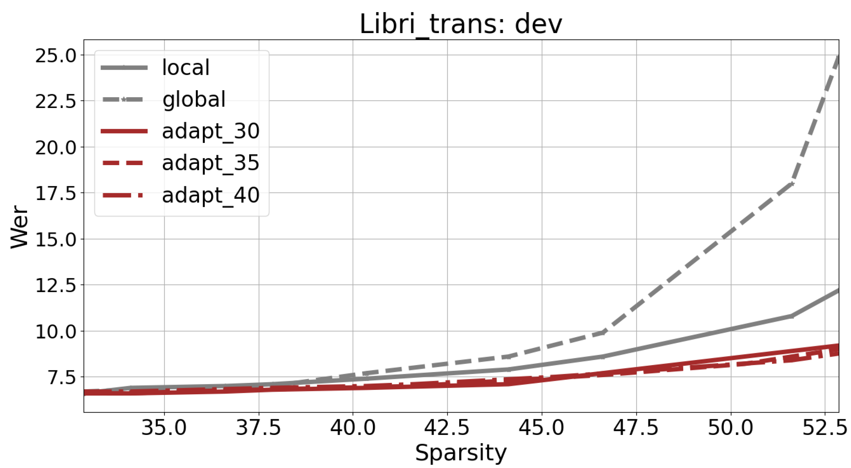
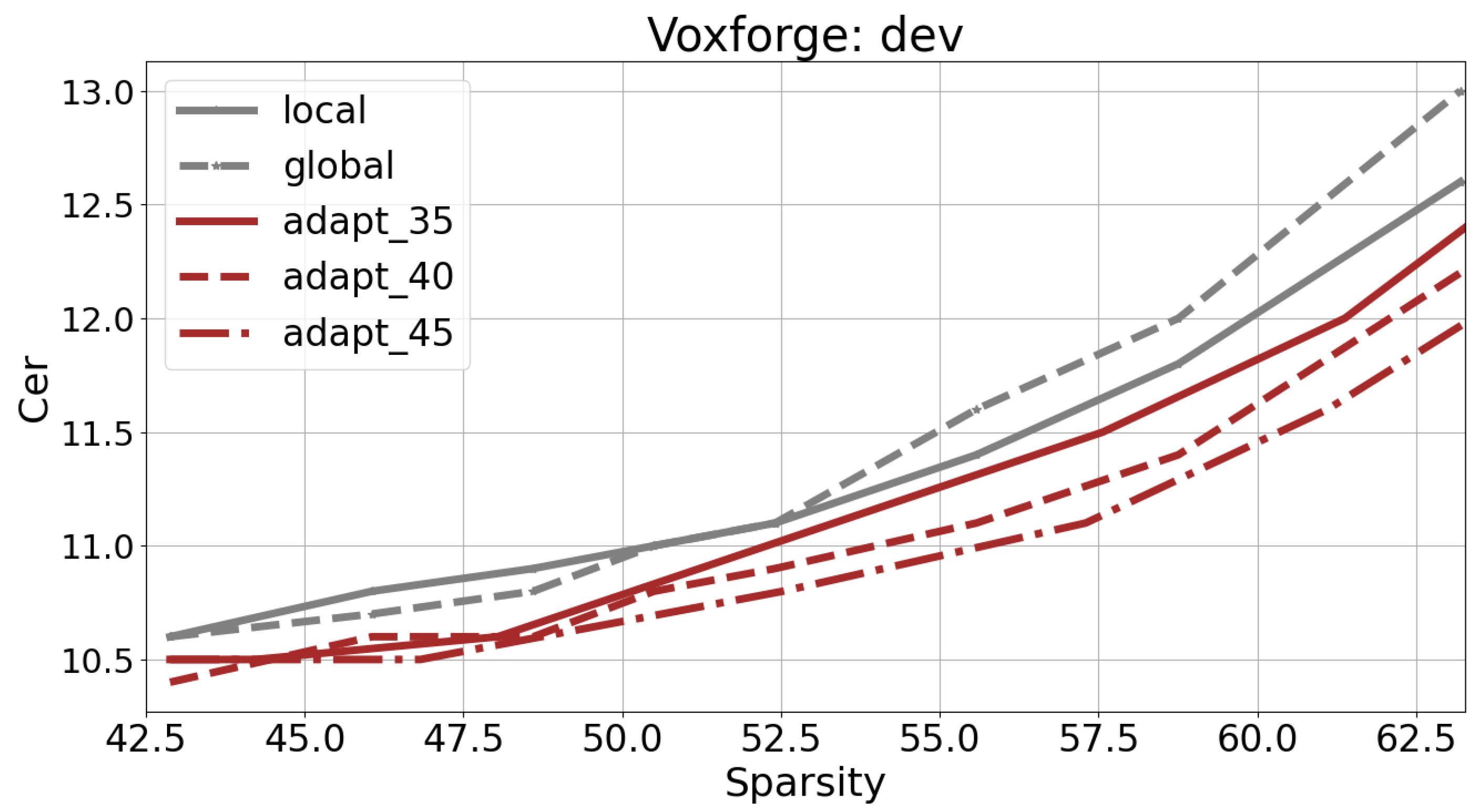
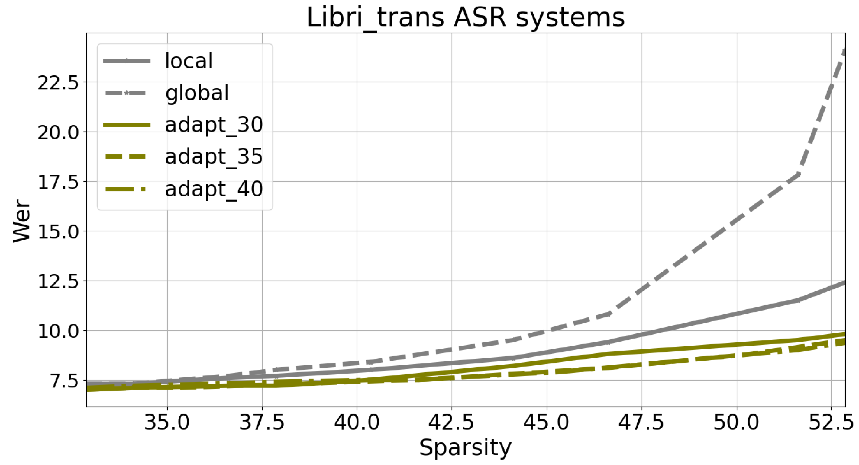
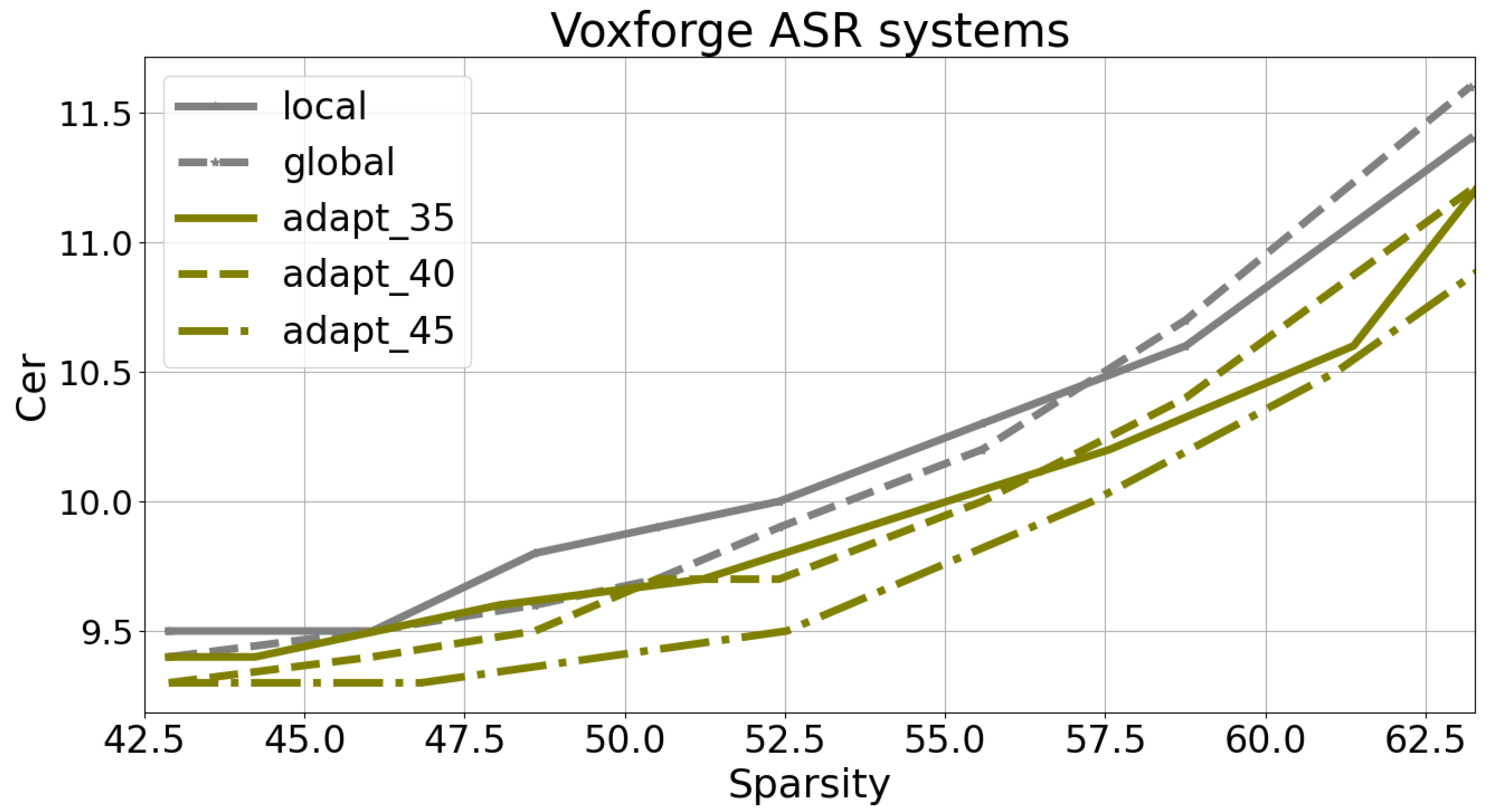
Figure 13 and Figure 14 present the error rates for varying Sparsity levels, reaching up to 52.5% for Libri-trans and 62.5% for VoxforgeIT. It is noteworthy that, beyond these thresholds, the application of global pruning results in a significant increase in the error rate. Specifically, the error rate exceeds 24% for Libri-trans and 13.9% for VoxforgeIT.

In all cases, variable scale pruning demonstrates superior performance compared with global and local pruning techniques.

The Word Error Rate (WER) of the non-pruned Libri-trans system is reported to be 6.6% in Section 3.2. According to Figure 13, when the WER is 7.3%, variable scale pruning achieves a Sparsity gain of 7%. This allows the model to be compressed to 52.5% while maintaining a WER of 8.9%. This corresponds to a relative increase in the error rate of approximately 13.5%.

>In Section 3.2, it is stated that the non-pruned VoxforgeIT system achieved a Character Error Rate (CER) of 9.3%. The information presented in Figure 14 clearly shows that, for a CER of 9.5%, the variable scale pruning models exhibit 6% higher Sparsity values compared with the locally or globally pruned models. Furthermore, when the pruned system achieves a Sparsity level of 57%, the CER remains at approximately 10%. As a result, we can deduce an absolute increase in the error rate of 0.7% when the model is compressed to 57%.

It is worth noting that VoxforgeIT’s transformer model demonstrates a higher level of over-parameterization compared with that of Libri-trans, as evidenced by its larger Sparsity at the same increase in error rate.

Overall, these results highlight the effectiveness of variable scale pruning in achieving a favorable trade-off between Sparsity and error rate for both datasets. Setting a maximum allowable relative increase of 10% in the error rate (i.e., WER = 7.3% for Libri-trans and CER = 10.3% for VoxforgeIT), the most optimal pairs of (error rate, pruning rate) were found to be (7.6%, 43%) for the Libri-trans system and (10.3%, 59.5%) for the VoxforgeIT system.

6. Conclusions and Future Work

This paper presents a novel approach for pruning transformer models in end-to-end speech recognition, addressing the significant complexity and size of these models that hinder their efficient deployment in Automatic Speech Recognition tasks. While transformer systems exhibit excellent performance, their large size poses challenges for practical implementation. In order to overcome this limitation, our work focused on studying and optimizing pruning techniques specifically tailored to the transformer architecture.

In this study, we devised a method that centers around analyzing the evolution of weights within the feedforward layers present in both the encoder and decoder blocks of the transformer. Through careful observation, we found that deeper layers tend to possess higher weights compared with earlier layers. Leveraging this insight, our proposed approach, named variable scale pruning, applies a pruning rate that decreases progressively as the layer depth increases.

To validate the effectiveness of our method, we conducted experimental evaluations on diverse databases. The results showcased the superiority of our approach over traditional local and global pruning methods. Remarkably, our technique achieved an impressive model compression rate of up to 59.5%, all while maintaining a less than 10% relative reduction in accuracy.

Looking ahead, there are exciting research directions to explore. One such avenue involves investigating the application of variable scale pruning on attention head layers, which play a vital role in the transformer’s performance. Additionally, we intend to delve into fine-tuning techniques for the pruned models, aiming to further optimize their performance without sacrificing compression gains. In the present era, there is a growing trend in the adoption of large and pre-trained models, known as foundation models. Through fine-tuning, these models continually improve their efficiency and hold a crucial advantage in being able to work with minimal labeled data. The pruning of such models offers a compelling and promising avenue for further research.

By advancing the field of transformer model pruning for end-to-end speech recognition, our work contributes to the broader goal of enabling the widespread adoption of efficient and high-performing transformer systems in real-world applications.

References

1. Vaswani, A.; Shazeer, N.; Parmar, N.; Uszkoreit, J.; Jones, L.; Gomez, A.N.; Kaiser, L.; Polosukhin, I. Attention Is All You Need. In Proceedings of the Advances in NIPS, 2017, Long Beach, CA, USA, 4–9 December 2017. [Google Scholar]
2. Han, S.; Pool, J.; Tran, J.; Dally, W.J. Learning both Weights and Connections for Efficient Neural Networks. In Proceedings of the Advances in Neural Information Processing Systems, Montreal, QC, USA, 7–12 December 2015; pp. 1135–1143. [Google Scholar]
3. Letaifa, L.B.; Torres, M.I. Perceptual Borderline for Balancing Multi-Class Spontaneous Emotional Data. IEEE Access 2021, 9, 55939–55954. [Google Scholar] [CrossRef]
4. Watanabe, S.; Hori, T.; Karita, S.; Hayashi, T.; Nishitoba, J.; Unno, Y.; Soplin, N.E.Y.; Heymann, J.; Wiesner, M.; Chen, N.; et al. Espnet: End-to-End Speech Processing Toolkit. In Proceedings of the INTERSPEECH, Hyderabad, India, 2–6 September 2018; pp. 2207–2211. [Google Scholar]
5. Rabiner, L.; Juang, B.H. Fundamentals of Speech Recognition; Prentice Hall: Hoboken, NJ, USA, 1993. [Google Scholar]
6. Dahl, G.E.; Yu, D.; Deng, L.; Acero, A. Context-Dependent Pre-Trained Deep Neural Networks for Large-Vocabulary Speech Recognition. IEEE Trans. Audio Speech Lang. Process. 2012, 20, 30–42. [Google Scholar] [CrossRef]
7. Li, S.; Raj, D.; Lu, X.; Shen, P.; Kawahara, T.; Kawai, H. Improving Transformer-Based Speech Recognition Systems with Compressed Structure and Speech Attributes Augmentation; INTERSPEECH: Graz, Austria, 2019; pp. 4400–4404. [Google Scholar]
8. Zouari, L.B. Embedded Real Time Speech Recognition System for Smart Home Environment. Int. J. Sci. Eng. Res. 2017, 8, 42–48. [Google Scholar]
9. Fan, A.; Grave, E.; Joulin, A. Reducing Transformer Depth on Demand with Structured Dropout. In Proceedings of the International Conference on Learning Representations, Addis Ababa, Ethiopia, 26–30 April 2020. [Google Scholar]
10. Li, Z.; Li, H.; Meng, L. Model Compression for Deep Neural Networks: A Survey. Computers 2023, 12, 60. [Google Scholar] [CrossRef]
11. Qi, J.; Du, J.; Siniscalchi, S.M.; Ma, X.; Lee, C.H. Analyzing upper bounds on mean absolute errors for deep neural network-based vector-to-vector regression. IEEE Trans. Signal Process. 2020, 68, 3411–3422. [Google Scholar] [CrossRef]
12. Qi, J.; Yang, C.; Chen, P.; Tejedor, J. Exploiting Low-Rank Tensor-Train Deep Neural Networks Based on Riemannian Gradient Descent With Illustrations of Speech Processing. IEEE/ACM Trans. Audio Speech Lang. Process. 2023, 31, 633–642. [Google Scholar] [CrossRef]
13. Letaifa, L.B.; Rouas, J.L. Transformer Model Compression for End-to-End Speech Recognition on Mobile Devices. In Proceedings of the European Signal Processing Conference, EUSIPCO, Belgrade, Serbia, 29 August–2 September 2022. [Google Scholar]
14. LeCun, Y.; Denker, J.; Solla, S. Optimal Brain Damage. In Proceedings of the Advances in Neural Information Processing Systems, Denver, CO, USA, 27–30 November 1989; pp. 598–600. [Google Scholar]
15. Kim, H.G.; Na, H.; Lee, H.; Lee, J.; Kang, T.G.; Lee, M.J.; Choi, Y.S. Knowledge Distillation Using Output Errors for Self-attention End-to-end Models. In Proceedings of the IEEE International Conference on Acoustics, Speech and Signal Processing ICASSP, Brighton, UK, 12–17 May 2019. [Google Scholar]
16. Noach, M.B.; Goldberg, Y. Compressing Pre-trained Language Models by Matrix Decomposition. In Proceedings of the International Joint Conference on Natural Language Processing, Suzhou, China, 4–7 December 2020. [Google Scholar]
17. Lu, Z.; Sindhwani, V.; Sainath, T. Learning Compact Recurrent Neural Networks. In Proceedings of the International Conference on Acoustics, Speech, and Signal Processing, Shanghai, China, 20–25 March 2016. [Google Scholar]
18. He, T.; Fan, Y.; Qian, Y.; Tan, T.; Yu, K. Reshaping deep neural network for fast decoding by node-pruning. In Proceedings of the IEEE International Conference on Acoustics, Speech and Signal Processing ICASSP, Florence, Italy, 4–9 May 2014. [Google Scholar]
19. Cao, S.; Zhang, C.; Yao, Z.; Xiao, W.; Nie, L.; Zhan, D.; Liu, Y.; Wu, M.; Zhang, L. Efficient and effective sparse LSTM on FPGA with Bank-Balanced Sparsity. In Proceedings of the Proceedings SIGDA International Symposium on FPGA, Seaside, CA, USA, 24–26 February 2019. [Google Scholar]
20. Chen, S.; Sun, W.; Huang, L. WHC: Weighted Hybrid Criterion for Filter Pruning on Convolutional Neural Networks. In Proceedings of the IEEE International Conference on Acoustics, Speech and Signal Processing ICASSP, Rhodes Island, Greece, 4–10 June 2023. [Google Scholar]
21. Han, S.; Pool, J.; Narang, S.; Mao, H.; Gong, E.; Tang, S.; Elsen, E.; Vajda, P.; Paluri, M.; Tran, J.; et al. DSD: Dense-sparse-dense training for deep neural networks. In Proceedings of the Proceedings ICLR, Toulon, France, 24–26 April 2017. [Google Scholar]
22. Bie, A.; Venkitesh, B.; Monteiro, J.; Haidar, M.A.; Rezagholizadeh, M. A Simplified Fully Quantized Transformer for End-to-End Speech Recognition. 2020. Available online: https://arxiv.org/pdf/1911.03604.pdf (accessed on 9 August 2023).
23. Letaifa, L.B.; Rouas, J.L. Fine-grained analysis of the transformer model for efficient pruning. In Proceedings of the International Conference on Machine Learning and Applications ICMLA, Nassau, Bahamas, 12–14 December 2022. [Google Scholar]
24. Peng, Y.; Sudo, Y.; Muhammad, S.; Watanabe, S. DPHuBERT: Joint Distillation and Pruning of Self-Supervised Speech Models. INTERSPEECH. arXiv 2023, arXiv:2305.17651. [Google Scholar]
25. Gupta, M.; Agrawal, P. Compression of Deep Learning Models for Text: A Survey. Comput. Sci. ACM Trans. Knowl. Discov. Data 2020, 16, 61. [Google Scholar] [CrossRef]
26. Anwar, S.; Hwang, K.; Sung, W. Structured Pruning of Deep Convolutional Neural Networks. ACM J. Emerg. Technol. Comput. Syst. 2017, 13, 32. [Google Scholar] [CrossRef]
27. Voita, E.; Talbot, D.; Moiseev, F.; Sennrich, R.; Titov, I. Analyzing Multi-Head Self-Attention: Specialized Heads Do the Heavy Lifting, the Rest Can Be Pruned. In Proceedings of the 57th Annual Meeting of the Association for Computational Linguistics, Florence, Italy, 28 July–2 August 2019. [Google Scholar]
28. Michel, P.; Levy, O.; Neubig, G. Are Sixteen Heads Really Better than One? In Proceedings of the Advances in Neural Information Processing Systems, Vancouver, BC, Canada, 8–14 December 2019. [Google Scholar]
29. Han, S.; Mao, H.; Dally, W.J. Deep Compression: Compressing Deep Neural Network with Pruning, Trained Quantization and Huffman Coding. In Proceedings of the ICLR, San Juan, Puerto Rico, 2–4 May 2016. [Google Scholar]
30. Molchanov, P.; Mallya, A.; Tyree, S.; Frosio, I.; Kautz, J. Importance Estimation for Neural Network Pruning. In Proceedings of the IEEE Conference on Computer Vision and Pattern Recognition CVPR, Long Beach, CA, USA, 15–20 June 2019; pp. 11264–11272. [Google Scholar]
31. Ganesh, P.; Chen, Y.; Lou, X.; Khan, M.A.; Yang, Y.; Sajjad, H.; Nakov, P.; Chen, D.; Winslett, M. Compressing Large-Scale Transformer-Based Models: A Case Study on BERT. Trans. Assoc. Comput. Linguist. 2021, 9, 1061–1080. [Google Scholar] [CrossRef]
32. Nazli, G.; Ankit, J.; Qian, S. Comparative analysis of sparse matrix algorithms for information retrieval. Computer 2003, 2, 0–4. [Google Scholar]
33. Amirshahi, A.; Klein, J.A.; Ansaloni, G.; Atienza, D. TiC-SAT: Tightly-coupled Systolic Accelerator for Transformers. In Proceedings of the 28th Asia and South Pacific Design Automation Conference, Tokyo, Japan, 16–19 January 2023; pp. 657–663. [Google Scholar]
34. Duff, I. A survey of sparse matrix research. Proc. IEEE 1977, 65, 500–535. [Google Scholar] [CrossRef]
35. Blalock, D.; Gonzalez Ortiz, J.J.; Frankle, J.; Guttag, J. What is the State of Neural Network Pruning? In Proceedings of the Machine Learning and Systems, Cambridge, MA, USA, 16–18 November 2020; Volume 2, pp. 129–146. [Google Scholar]
36. See, A.; Luong, M.T.; Manning, C.D. Compression of Neural Machine Translation Models via Pruning. In Proceedings of the SIGNLL Conference on Computational Natural Language Learning, Berlin, Germany, 11–12 August 2016; pp. 291–301. [Google Scholar]
37. Dong, L.; Xu, S.; Xu, B. Speech-Transformer: A No-Recurrence Sequence-to-Sequence Model for Speech Recognition. In Proceedings of the IEEE International Conference on Acoustics, Speech and Signal Processing, Calgary, AB, Canada, 15–20 April 2018. [Google Scholar] [CrossRef]
38. Kocabiyikoglu, A.C.; Besacier, L.; Kraif, O. Augmenting Librispeech with French Translations: A Multimodal Corpus for Direct Speech Translation Evaluation. In Proceedings of the LREC, Miyazaki, Japan, 7–12 May 2018. [Google Scholar]
39. Voxforge (Italian). 2019. Available online: http://www.repository.voxforge1.org/downloads (accessed on 17 August 2023).
40. Panayotov, V.; Chen, G.; Povey, D.; Khudanpur, S. LIBRISPEECH: An ASR corpus based in public domain audio books. In Proceedings of the ICCASP, South Brisbane, QLD, Australia, 19–24 April 2015. [Google Scholar]
41. Ko, T.; Peddinti, V.; Povey, D.; Khudanpur, S. Audio Augmentation for Speech Recognition. In Proceedings of the INTERSPEECH, Dresden, Germany, 6–10 September 2015. [Google Scholar]
42. Povey, D.; Ghoshal, A.; Boulianne, G.; Burget, L.; Glembek, O.; Goel, N.; Hannemann, M.; Motlicek, P.; Qian, Y.; Schwarz, P.; et al. The Kaldi Speech Recognition Toolkit. In Proceedings of the IEEE Workshop on Automatic Speech Recognition and Understanding, ASRU. IEEE Signal Processing Society, Waikoloa, HI, USA, 11–15 December 2011. [Google Scholar]
43. Kingma, D.P.; Ba, J.L. ADAM: A Method for stochastic Optimization. In Proceedings of the International Conference on Learning Representations, Banff, AB, Canada, 14–16 April 2014; pp. 1–13. [Google Scholar]
44. Bérard, A.; Besacier, L.; Kocabiyikoglu, A.C.; Pietquin, O. A comparative study on transformer vs. RNN in speech applications. In Proceedings of the IEEE International Conference on Acoustics, Speech and Signal Processing, Brighton, UK, 12–17 May 2019. [Google Scholar]
45. Karita, S.; Chen, N.; Hayashi, T.; Hori, T.; Inaguma, H.; Jiang, Z.; Someki, M.; Soplin, N.; Yamamoto, R.; Wang, X.; et al. End-to-End Automatic Speech Translation of Audiobooks. In Proceedings of the Automatic Speech Recognition and Understanding ASRU, Calgary, AB, Canada, 15–20 April 2018. [Google Scholar]
Figure 1. The different pruning structures: (a) no pruning (b), unstructured pruning (c), neuron pruning (d), block pruning (e), layer(s) pruning.
Algorithms 16 00398 g001
Figure 2. Local pruning (on the left) versus global pruning (on the right).
Algorithms 16 00398 g002
Figure 3. ASR transformer main components.
Algorithms 16 00398 g003
Figure 4. The distribution of attention, feedforward, and other layer parameters between the encoder and decoder of the Libri-trans and VoxforgeIT models. Other layers are the embedding, input and output, and normalization layers.
Algorithms 16 00398 g004
Figure 5. Evolution of the weight magnitude (× 10 5 ) of the FF1 layers through the encoder blocks of the Libri-trans model.
Algorithms 16 00398 g005
Figure 6. Evolution of the average magnitudes of the FF1 and FF2 layer weights through the encoder blocks of the VoxforgeIT model.
Algorithms 16 00398 g006
Figure 7. Evolution of the average magnitudes of the FF1 and FF2 layer weights through the decoder blocks of the VoxforgeIT model.
Algorithms 16 00398 g007
Figure 9. Error rate as a function of global and local pruning rate for the Libri-trans system.
Algorithms 16 00398 g009
Figure 10. Error rate as a function of global and local pruning rate for the VoxforgeIT system.
Algorithms 16 00398 g010
Figure 11. The development error rate is plotted as a function of Sparsity for the Libri-trans system after applying local, global, and variable scale pruning techniques.
Algorithms 16 00398 g011
Figure 12. The development error rate is plotted as a function of Sparsity for the VoxforgeIT system, after applying local, global, and variable scale pruning techniques.
Algorithms 16 00398 g012
Figure 13. The test error rate is plotted as a function of Sparsity for the Libri-trans system after applying local, global, and variable scale pruning techniques.
Algorithms 16 00398 g013
Figure 14. The test error rate is plotted as a function of Sparsity for the VoxforgeIT system after applying local, global, and variable scale pruning techniques.
Algorithms 16 00398 g014