Abstract
Modeling the spread of infections in networks is a well-studied and important field of research. Most infection and diffusion models require a real value or probability at the edges of the network as an input, but this is rarely available in real-life applications. The Generalized Inverse Infection Model (GIIM) has previously been used in real-world applications to solve this problem. However, these applications were limited to the specifics of the corresponding case studies, and the theoretical properties, as well as the wider applicability of the model, are yet to be investigated. Here, we show that the general model works with the most widely used infection models and is able to handle an arbitrary number of observations on such processes. We evaluate the accuracy and speed of the GIIM on a large variety of realistic infection scenarios.
1. Introduction
Infection models are frequently used in many real-life applications in sociology, economics and epidemics. A large variety of models are available for different applications, the most popular ones being compartmental models and their variants [1,2]. They are regularly used to model infectious diseases [2], the spread of information and behavior on social networks [3], or the spread of economic events [4,5,6,7]. Some of the tasks associated with these models include influence maximization, that is, finding the set of individuals yielding the largest expected infection [8,9,10,11], or the prediction of a posteriori infection values, i.e., finding the probability of infection for all nodes of the network [12]. Many infection models are network-based; they assume a set of nodes and the connections between them to be given. Most also assume a specific value to be available on the links of the networks; these are called edge infection values, and they represent the probability that the infection spreads from one node to another.
A common challenge in the application of infection models is the lack of information on the edge infection values on the links of networks. Recently, several authors have proposed models to estimate these values. Many of the models assume that the time stamps of the infection for each node are given [13,14,15,16,17,18,19,20], although some approaches do not require this property [21,22,23]. Current estimation methods are based on a variety of infection models [15], but most often, the SIR model or one of its variants is used [16,17,18,21]. Most of these models were developed independently of each other, and most of them take a different, often application-specific approach to the problem.
The Generalized Inverse Infection Model (GIIM) was recently proposed to solve the problem of estimating edge infection probabilities in two case studies. The model was applied to estimate the risk of infection between geographical regions during (1) the 2009 H1N1 pandemic in Sweden [24] and (2) the 2016 Zika outbreak in the Americas [25]. In both cases, the model was able to formulate edge infection values as a function of known disease-relevant attributes, such as socioeconomic, climate and travel determinants, and was also shown to have good predictive capabilities.
The properties of the GIIM have only been described within the strict boundaries of these two case studies, however. As such, there is no existing scientific work that examines the theoretic properties and general applicability of the model. In this paper, we show that:
- The GIIM can account for an arbitrary number of observations on the infection process.
- The GIIM allows for flexibility in the type of observations provided as input.
- The GIIM allows for flexibility in the underlying infection model.
An infection-spreading process may be fully or partially observable. The GIIM is able to handle an arbitrary number of observations on such processes, enabling it to adapt to the specific requirements of applications. In this paper, we experiment with the two extremes of such requirements. In fully observed scenarios, we know at exactly what time a node was infected. In two-observation cases, we can only observe who was infected at the beginning and at the end. Both fully observed and two-observation approaches and any in between them can be naturally formulated in the framework of the GIIM.
Observations on the infection process might be available in various forms, so the model should be flexible enough to handle different forms of input data. Two types of observations are investigated in this paper. The first one is based on the common assumption that at a certain time step, we know which nodes were infected and which nodes were not. In the second type of observation, we have real values indicating how likely it is for the nodes to become infected at a given time step. We propose additional types of observations that we plan to investigate in future work.
Another key advantage is the freedom to choose the underlying infection model. Most of the existing approaches are designed with a single infection model in mind, most often a compartmental infection model, such as the SEIR model or one of its variants. In contrast, the GIIM makes the inverse infection tasks independent of the infection model. We show that the SI, SIR and SEIR models can be used within the GIIM framework, making the GIIM compliant with most of the infection models used in the literature.
Lastly, the GIIM is able to directly estimate real edge infection values, as well as functional forms, which include variables representative of vertex and edge attributes.
In this paper, we evaluate the features of the GIIM highlighted above using a large variety of artificial infection scenarios. The scenarios differ in graph classes, the size of the underlying graphs, the size of the outbreak, the type of infection models used and the type of performance evaluation. Additionally, both fully and partially observed scenarios are considered with real and binary observations. Our goal is to analyze the behavior of the GIIM in the above examples in terms of the general tractability of the tasks and the accuracy of the predictions.
The rest of the paper is organized as follows. In Section 2, we review some basic graph-theoretic concepts and define the used infection models and the General Inverse Infection Model. In Section 3, we examine the various types of observations used in the model, explore possible ways to measure the goodness of the results and describe the optimization method itself. We also discuss a special case of the GIIM. In Section 4, we evaluate the performance of a number of specific variations of the general model. First, we examine the tractability of the task on trees and directed acyclic graphs, and then we use a large variety of artificially generated infection scenarios and complex networks to test the accuracy of our model. Finally, the scalability of the model is tested on large complex networks. We close our discussion with a short description of some features of the GIIM that are not investigated in this paper, present some of the challenges posed in this study and discuss possible ways to further expand the functionality of our model.
2. Definitions
The infection processes described in this paper take place in graphs. We will denote graph G as , where is the vertex and is the edge set of G. By default, we are going to consider these graphs to be connected and undirected, unless otherwise noted. The infection models require a real value (also denoted by ) to be present on all edges of the graph; these are known as the edge infection probabilities. We will denote the surjective assignment of edge infection probabilities to the edges as . The task of inverse infection is the estimation of these values.
Among the most frequently used infection models present in the literature are the IC, SI, SIR and SEIR models [1,2,9]. These processes are iterative; events take place in discrete time steps, and the models terminate in finite steps.
2.1. Infection Models
Discrete infection models work by assigning states to the vertices of the graph. Each vertex may only be in one state at a given time, and all vertices must be in a state at all times. The states of the above models are susceptible (S), exposed (E), infected (I) and removed (R). The exposed and infected states have discrete time periods attached to them, and we denote these by and . Infected nodes attempt to infect their susceptible neighbor nodes according to the corresponding edge weight probability . If successful, the newly infected nodes transition into an exposed state for iterations, after which they attempt to infect susceptible neighbors for iterations, after which point they become removed (dead or immune) and can no longer infect other nodes. The models differ in complexity, with the most complex being the SEIR model, which has all of the above states; in the SIR model, ; in the IC model, and ; and in the SI model, and . Correspondingly, in the IC, SI and SIR models, the nodes are never in an exposed state, and in the SI model, the nodes are never removed; i.e., they may attempt to infect neighboring nodes indefinitely.
We illustrate the mechanics of the infection process on the most general infection model, SEIR. Apart from the network itself, the infection process of the SEIR model has two inputs. The first is the assignment of edge infection probabilities for all edges. The second is the set of initially infected nodes . These nodes are considered to be infected at the start of the process. Let be the set of nodes in the infected state in iteration i. Each node tries to infect its susceptible neighbors v according to ; if the attempt is successful, v will begin its exposed period. If more than one node tries to infect v in the same iteration, the attempts are made independently of each other in an arbitrary order within the same iteration. Still, in iteration i, the status of infected nodes changes to removed if the difference between i and the time of their infection becomes greater than ; exposed nodes become infected when the difference becomes greater than . The process terminates in iteration t if the set of infected and exposed nodes is empty. In a finite network, the process always terminates in a finite number of steps.
The other infection models behave similarly, with minor differences. The SEIR infection processes take longer to complete because the nodes have to spend time in an exposed state before becoming infectious. Similarly, higher corresponds to more infected nodes because there are more opportunities to infect neighboring nodes. Finally, in the SI model, given enough time, all vertices become infected with a probability of one if there is an initially infected node in every connected component.
2.2. General Inverse Infection Model
The Generalized Inverse Infection Model formalizes the estimation of edge infection values as a general optimization problem by defining the inputs and outputs of this task and describing the relationship between the infection and edge infection estimation models [24,25]. We assume that the underlying graph of the infection process is known. We also assume that we have observations on an infection process taking place in the network. The observations on the infection process are given in the form of , where denotes a time stamp. Each assigns an observation on the infection process at time step t to all nodes of the network. Set O contains all observations, and set T contains all time stamps. At least two observations are needed to provide a meaningful model, but otherwise, the number of observations required is not specified. Previous applications of the GIIM always considered observations to be available at all [24,25]. Finally, we assume that we know the specific type of infection process taking place in the network, although in Section 5, we will discuss what happens if we relax this assumption.
We define the inputs of the GIIM as follows: we have an unweighted graph G, an infection model , the set of sample times T and the observations on the infection process for all , where . We denote the unknown weight assignment to the edges of the graph by , and for now, we assume to be any network-based infection model from Section 2.1. We can interpret as a procedure that makes observations at time steps T on infection process taking place in graph G with edge weights , . We also define a difference function d that compares two observations: . The task of the GIIM is to find an estimation of W so that between O and is as small as possible: we are looking for an edge infection probability assignment that best explains the observations of the original infection process.
Finally, we define the General Inverse Infection Model as:
General Inverse Infection Model: Given an unweighted graph G, an infection model , a set of sample times T and observations , we seek the edge infection probability assignment such that the difference between O and is minimal.
The definition above defines the inverse infection task as an optimization problem: the minimization of the error between a reference and a computed observation. The optimization task itself would be an iterative refinement of the computed observation. The solution procedure proceeds as follows: begin with an initial weight configuration , run the infection model, extract observations , compute the error between O and , and then refine and repeat the process until the error is less than an accuracy constant a selected by the user. Algorithm 1 summarizes the main components of the GIIM. The specific search strategy that we implement in this paper to refine is the Particle Swarm Optimization method [26], but other methods may be selected if they follow the structure above. The search process can be easily implemented in a parallel way. Given multiple candidate weight configurations, multiple instances of the infection models can be computed independently of each other on multiple threads.
| Algorithm 1 Generalized Inverse Infection Model |
|
It should be noted that depending on the application, the weight assignment function W may also be time-dependent; i.e., the weights themselves may change in time. As this scenario was already investigated in [24,25], we will treat all edge weights and W as static in this paper.
Function Estimation
Finding an edge weight assignment that minimizes the difference between the reference and computed infections can be computationally expensive, as we will see in Section 4, as this requires finding the edge infection probability for all edges of the graph.
Another approach to direct edge weight estimation is to compute the edge weights as a function of existing attributes, as seen in [4,23,24,25]. These works propose that additional information can be assigned to the edges or vertices of the graph. Examples include the number of passengers or travel distance in an air traffic network [25] or the number or frequency of transactions [4]. The edge infection probabilities themselves can be defined as functions of these attributes, in which case, the optimization task changes to finding the proper function formulation explaining the reference infection process. This approach is often an easier estimation task compared with finding all of the edge weights.
As the function estimation approach has already been investigated in [24,25], we refer the reader to these works for further information.
3. Properties of GIIM
In this paper, we demonstrate the general applicability and performance of the model under its three flexible properties: the availability of observations, the type of observations and the type of underlying infection model. Two different error functions are considered to quantify the model performance.
3.1. Observations
In the definition above, O is defined as a set of vectors for all , and each vector assigns an observation to all vertices of the graph at a specific time step t. Since T represents the set of sample times, it is safe to assume that it can be ordered; thus, the set of observations can also be ordered according to T. The cardinality of T is not specified, but at least two time samples are needed to make a meaningful prediction for W. The upper limit is application-dependent. In the case of a discrete-time infection model, T usually contains natural numbers.
We define as the time period of the reference infection process. We assume this process to be finite, as described in Section 2.1. If the infection model is finite, i.e., it finishes at iteration , it is meaningless to make observations after because the process does not change after .
From a practical perspective, the first and last observations—at and , respectively—give bounds, since we do not have other observations apart from the ones at T. Therefore, if we want to explain the witnessed infection scenario, we should consider and to be the beginning and the end of the infection process.
The task of the GIIM is to find an edge weight configuration that explains the original observed infection process. Therefore, the set of observations O should contain information that represents the behavior of nodes in the infection process. In this paper, we suggest two extreme cases of observation levels, but the proposed framework is able to handle other types as well. Realistic cases may be in between these two extremes, all of which can be accommodated within the modeling framework.
- Two observations are available at and .
- Observations for all iterations of the discrete infection process are available T.
The set of observations O should contain information that represents the behavior of nodes in the infection process. In this paper, we suggest two specific types of observations that can be made.
The first observation type defines the observations as real values between 0 and 1, which are assigned to each node at the time steps where observations are available. For this type of observation, for time step t and node v, the value represents the likelihood that node v is infected at time step t, i.e., the cumulative infection probability of v up to time step t, while represents the vector of observations for all nodes at time step t. The initial infections, the probability that is infected before the process, are stored in , while the probability that a node becomes infected measured at the end of the process is in , corresponding to the a priori and a posteriori distributions assumed known in the two-observation case. For finite infection models, if we limit our viewpoint to a single node, the series of observations, , will be a monotonically increasing function since starts at the initial infection probability , and the infection process may never decrease this value.
Another way to make observations is to simply consider flags on the nodes signaling whether they have been infected or not. In this case, for a node , indicates that it has not been infected up to time step t, and means that it is already infected at t. This approach is the most common in the literature [15,16,17,24,25]. It can be used directly, or if time stamps are available on the nodes, we can simply consider if and if , where denotes the time at which a node was infected.
3.2. Error Function
The chosen error function should be able to compare observations made on the infection process. The observations are a set of vectors with time stamps attached to each vector. We can pair the vectors according to their time stamps, compute the error and then aggregate the individual distances into a single value.
If the observations are vectors containing real numbers, a form of vector distance should be a natural choice. For the continuous-valued observation type presented in the previous subsection, we use the root-mean-squared error (RMSE) function to compare the individual observation vectors. For binary observations, ROC evaluation is used in a similar fashion.
3.3. Computation
The GIIM defines a general optimization task, which can be solved with the iterative refinement of an initial edge weight configuration. The number of edges, even in a medium-sized graph, can be in the tens or hundreds of thousands, so finding the proper combination of weights can be challenging; therefore, choosing an appropriate optimization method is crucial. Here, we recommend and use the Fully Informed Particle Swarm method of Kennedy and Mendes [26,27], which has proved successful in previous inverse infection tasks [4].
The optimization task was defined in Section 2.2 as the minimization of the error between computed and reference observations. The method is initialized with randomly selected edge infection values within reasonable bounds, and then a simulation of the infection process is computed to create observations. The error between the reference and computed observations is counted and used to adjust the edge infection values. The process is then repeated.
The search strategy is Particle Swarm Optimization: an iterative multi-agent non-gradient metaheuristic. Each agent has a position that represents an edge weight configuration, and the agents refine their positions by interacting with their neighbors. This is implemented by adding the velocity of the agent to the position of the agent. The velocity of the agent is computed from its previous value, the best result found by the agent and its neighbors and a random vector. The goodness of an agent is the goodness of the edge weight configuration it represents, and the goodness is evaluated by running an infection model and computing the error of the resulting observations. The agents are connected to each other through a pre-defined topology describing the neighborhood of each agent.
The specifics of the update rules for the positions and velocities, as well as the agent topology, are not fixed; there are several approaches in the literature. Here, like in [23], we follow the recommendations of Kennedy and Mendes [26] by adopting a von Neumann neighborhood for the agents and the following update rules:
where and denote the coordinate and velocity of particle i, is a uniform random number generator, is the best location found so far by particle i, is the number of neighbors that i has, and is the nth neighbor of i. The formula has two parameters: is the constriction coefficient, and is the acceleration constant. Again, we use the recommendations of Kennedy et al. and set and .
At the beginning, the positions of the agents are initialized with random values, and the velocities are set to zero. Then, at the end of each iteration, the positions and velocities are updated synchronously according to the above equations. The search is stopped if the method does not find a better global result in a set number of iterations. Algorithm 2 gives an outline of PSO.
| Algorithm 2 Particle Swarm Optimization |
|
The above algorithm can be implemented in a parallel way. Since the positions and velocities of each agent are updated at the end of each iteration, the goodness of the current position of each agent can be computed independently and simultaneously on multiple threads. This way, the running time of the algorithm can be significantly decreased in multi-core processors.
3.4. IIP as a Special Case of GIIM
The Inverse Infection Problem (IIP), as appeared in [22,23], can be considered the predecessor of the GIIM. The GIIM uses the same FPSO optimization method as the IIP, and the RMSE error function is one method used to guide the search in both models. However, compared with the GIIM, the IIP is much more limited in terms of scope. In the GIIM, a range of observation levels can be accommodated, and thus, the error function has to be extended to account for multiple real vectors. Additionally, the IIP fixes the number of observations to two: the a priori observation at time point zero and the a posteriori observation after the infection process concludes. The nature of the observation is also fixed: the IIP uses real infection values for the nodes: the probabilities of infection before and after the infection process. The IIP is also only applicable to one type of infection model, the Generalized Cascade Model [28], which is a variant of the IC model. In contrast, the GIIM handles an arbitrary number of observations, does not constrain the type of these observations and does not specify the used infection model.
4. Evaluation
The GIIM was designed to be a versatile tool that is easy to adapt to real-life problems. As we have seen in the previous section, it offers flexibility in terms of input data (number and type of observations), error function and infection model. Investigating all possible combinations of these is beyond the scope of this paper; instead, here, we focus on properties best tested on artificial infection scenarios. We measure the difficulty of a variety of inverse infection tasks in terms of the accuracy and the speed of the estimation. The tasks vary based on the number and type of available observations, the infection model and the prevalence of infections in the graph.
We present the evaluation in three parts. Section 4.2 focuses on the feasibility of the estimation on simple graph classes, namely, trees and directed acyclic graphs. We point out some trivial and non-trivial properties of the problem. In Section 4.3, we test the general applicability of the method on complex networks. Here, we consider a number of infection scenarios with different transmission probabilities between nodes, the prevalence of initial infections, infection models and their parameters. We also examine how the number of available observations affect the quality of the estimations. In Section 4.4, we consider the scalability of the method on large networks and the stability of the optimization method.
4.1. Method Details and Experimental Setup
The inverse infection tasks in this paper were constructed according to the following procedure.
- For a given graph, reference edge weights and the initially infected vertices are selected. The reference edge weights are not used in the inverse infection model, so they are omitted afterward.
- An infection model is selected and simulated using a modified version of CompleteSim, published in [28]. The original method computes two observations for the IC model, but it is easy to adapt it to other models. The set of infection models considered includes:
- (a)
- The Independent Cascade Model (SIR with ).
- (b)
- The SIR model with a infectious period.
- (c)
- The SEIR model with latency and a infectious period.
- (d)
- The SI model.
- During the simulation process, the set of reference observations for all nodes is computed. The observations are taken at the following time steps:
- (a)
- Two observations are available at and .
- (b)
- Observations for all iterations of the discrete infection process are available .
- Observations may be in the following form:
- (a)
- for all , that is, real infection values for all vertices of the graph denoting the probability of infection up to time step t. T may contain an arbitrary number of observations with respect to the restrictions in Section 3.1.
- (b)
- for all , that is, binary flags for all nodes of the graph signaling that the node was in an infectious state at time step t. T may contain an arbitrary number of observations with respect to the restrictions in Section 3.1.
- An error function is attached to the task.
- (a)
- The RMSE function averaged over all real-valued observations.
- (b)
- The ROC AUC value for the last observation with binary observations.
- The Particle Swarm Optimization method computes the estimated edge infection probabilities and observations. The method is used with the number of agents ranging from 100 to 250 depending on the size of the task. The method is stopped if it does not find a better solution in 50 iterations. We experimented with other settings and found that the accuracy of the method cannot be significantly improved by increasing the PSO parameters.
The final error value measures the goodness of the estimation. This procedure is repeated for a range of graph classes, sizes and infection scenarios.
4.2. Acyclic Examples
We examine two specific graph classes in this section, trees and directed acyclic graphs, to highlight certain non-trivial properties of the problem, but it is worth noting that fully observed finite infection processes (with time stamps for each node) can be naturally represented as DAGs. Our goal here is to find out how difficult it is to compute inverse infection tasks for these seemingly simple graph classes.
4.2.1. Underdetermination
A significant challenge exists in the estimation of edge infection values, which is illustrated using the following small example. Consider the example network in Figure 1a. There are two vertices, A and B, connected by a directed edge pointing from A to B. A and B are infected in succeeding iterations, A in and B in , and therefore, both have an observed binary flag of one. For the sake of simplicity, we consider the IC infection model. The best and optimal way to explain this scenario is to consider the connecting edge to have an infection probability of one. This is obviously an artifact arising from the available observations, a lack of information, since we have only one observation on a highly stochastic process. From the optimization point of view, however, this is an optimal solution to the scenario, since this is the most likely explanation of the observations. If we have real-valued observations on vertices A and B, the edge infection probability is the one satisfying the equation , where and denote the probability that A and B are infected. Next, consider the case shown in Figure 1b. There are now two possible sources of infection for B. Vertex A and vertex C both have a directed edge pointing toward, B and both were infected in the iteration before B was infected. Suppose that and are independent of each other. This way, . If the edge infection probabilities are real, there are many, possibly infinite ways of explaining this event, and this occurs at both binary flags and real -s. The challenge in accurate edge weight estimation again arises from a lack of information: we cannot decide the value of one edge value without knowing the other. Similar phenomena can be observed in the other infection models.
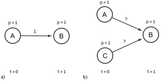
Figure 1.
Example of underdetermination. There is only one edge weight that explains the infection event on (a), while (b) is underdetermined.
We will refer to the problems above as the underdetermination of the inverse infection task. Underdetermination occurs in most real-life examples, even when the infection process is completely observable.
4.2.2. Trees and Directed Acyclic Graphs (DAGs)
We first evaluate the performance of the GIIM with arborescences. In these graphs, the infection spreads from the root, which is infected with probability of 1. Reference edge values were drawn from a uniform distribution between 0 and 1.
We consider both binary and real vertex infection values for three binary trees with heights of 4, 8 and 11 and two DAGs with 42 and 420 edges.
First, consider the task where we only have two observations on the infection process, one at the beginning and one at the end of the process. The accuracy of the estimations are presented in Table 1. The differences between infection models was minimal; therefore, results are only shown for the IC infection model. When the observations are provided as binary flags, the optimization algorithm is always able to find an optimal solution with RMSE = 0 and AUC = 1 much faster than with the real-valued solution. The reason for this is due to the underdetermination. If the observations are vectors of ones and zeros, the best way to explain the observations is to assign the edge values to be ones and zeros. To further illustrate this concept, consider the example shown in Figure 2. A leaf node in the tree has an observed infection value of one if all the edges leading to the leaf from the root have an edge infection value of one. If a leaf node has a value of zero, at least one edge connecting it to the root must have a zero value. This constrains the search to binary values as opposed to the continuous values of the real-valued case. Even if the behavior of the infection process is more complicated in DAGs, i.e., there are more explanations, this makes the binary inverse infection task much easier.

Table 1.
Average error of the optimization method on trees and directed lattices of various sizes for the two-observation case. The graph class, the number of edges and the accuracy of the results (error at the end of the optimization process) can be seen. Both binary and real-valued observations were tested, with AUC and RMSE provided for the former and only RMSE for the latter. Results are provided for the IC infection model.
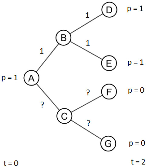
Figure 2.
Example of underdetermination. A leaf node has an observed infection value of one if and only if all the edges leading to it have edge infection values of one. A leaf node has an observed infection value of zero if at least one edge connecting the root to it has a value of zero.
Table 1 shows that in the two-observation real-valued case, the second DAG with 420 edges is more challenging than the similarly sized tree with 511 edges. This is because in the trees, there is only one path from the source of the infection to each node, so there is only one way to explain the process, while in the DAGs, multiple paths are present, meaning that there are multiple optima. The first problem is therefore easier than the second, hence the difference in the real-valued RMSE results in Table 1.
If the infection process is fully observed, i.e., if the infection status at all time steps is available, the error on all nodes for each individual time step can be computed separately; therefore, it is possible to measure the performance of the optimization method in each iteration of the infection process. Figure 3 shows the results for the fully observed case for the second tree and the second DAG. Since the root is the source of the infections and there are no directed cycles, an observation at time step i defines the infection values for nodes that are up to i distance from the root. The error steadily increases as the infection extends further from the root: at the last observation, the RMSE value is much greater than the value measured in the two-observation case. This increase in error is because the longer the chain of infections leading to a node, the more difficult it is to estimate its value. A possible reason for this is that the error becomes “spread out” equally among observations. In other words, the first few time steps are easier to compute because the nodes at a short distance from the root are far less numerous than the ones farther away. Additionally, the chain of edge infection values connecting them to the root is shorter, so there are fewer values to estimate.
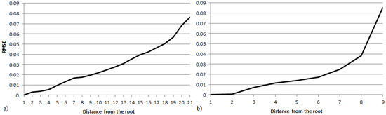
Figure 3.
The RMSE at different distances from the source in the fully observed IC model for (a) the second DAG and (b) the second tree in Table 1.
From the pure optimization perspective, the task is somewhat difficult, since the number of parameters to estimate—the number of edges—can be large. The PSO method required between 100 and 1500 iterations to find the above solutions, with the larger graphs taking more time and iterations, but there was minimal difference between the accuracy of the results, further illustrating the stability of the chosen method. The SIR and SEIR models took slightly more time to compute than the IC due to the longer and more complex infection process (non-zero and ).
4.3. Complex Networks
In addition to trees and DAGs, we also examine the performance of the GIIM on a more general complex network structure and under several different infection scenarios. The graph in question is undirected, and it has 250 nodes and 897 edges. The graph was created with the forest fire model [29]. The network itself is relatively small in network science terms, but our task here is to find the correct value for each edge, which is moderately challenging for the optimization algorithm. We examine the scalability of the method in the next section.
Our goal in this section is to compare the performance of the method in terms of accuracy and running time under a number of fundamentally different infection scenarios. The scenarios differ according to the infection model, the type and number of observations, the fraction of initially infected nodes and the size of the reference edge infection values. We measure the RMSE of real-valued observations and the ROC AUC of binary ones and consider minimally and fully observed cases as defined in Section 4.1. The scenarios examined are summarized as follows:
- Four different infection models: IC, SI, SIR with , and SEIR with and .
- Three sets of initially infected vertices: 33%, 10% or 2% of the nodes are initially infected with node infection probabilities ranging between 0 and 0.5 for the real-valued case and uniformly 1 for the binary case.
- Three sets of reference edge infection values as defined in Section 4.1. The values were drawn from a uniform random distribution between 0 and 0.25, 0 and 0.5, and 0 and 0.75.
If we only consider the infection scenarios, we have tasks, and if we add the observation types, this goes up to 108. Each of these tasks was computed ten times, and the results were averaged. The standard deviation measured between results was below 10% for all infection scenarios.
The RMSE and the AUC values are presented for the real-valued and binary infection tasks, respectively, for the two-observation case (, ) in Table 2. The results can be seen for all four of the infection models and all possible initial infection states and infection probability combinations. In the first column, the first number denotes the percentage of initially infected nodes, and the second one indicates the maximum value of the edge infection probability. In the SI model, the second observation was selected so that the estimated average node infection value at the observation was close to the estimated average node infection value at the last of observation of the SEIR model. As we saw in the previous section, the binary tasks are much easier to compute than the real-valued scenarios. Based on the results in Table 2, the larger infections are easier to predict. The reason for this is that the infection probability of a node is bounded: no matter how dense the infections are, the node infection probability cannot be greater than one. This means that if the infections are dense—either because there are many initially infected nodes, or the edge infection probabilities are large—a sizable fraction of the nodes are going to have an infection value close to one. This makes their distribution more homogeneous, and this also makes the optimization task easier, since there are fewer distinct values to estimate.
Table 2.
Accuracy of the optimization method for complex networks for the two-observation case. RMSE is shown for the real-valued case, and AUC is shown for the binary one. The numbers of the inverse infection tasks correspond to the scenarios described in this section. The first number denotes the percentage of initially infected nodes, and the second one indicates the maximum value of the edge infection probability.
The difference between the infection models is deceptive. Since we are running the same infection tasks on the same network with different infection models, if we increase the infectious period, we can expect a greater prevalence of vertex infections; therefore, we are seeing the same phenomenon as with the size of infections. To confirm this, we show the average infection probability of the nodes for the different tasks in Table 3.
Table 3.
Average node infection value for the last observation for all infection models. As before, the numbers of the inverse infection tasks correspond to the scenarios described in this section. The first number denotes the percentage of initially infected nodes, and the second one indicates the maximum value of the edge infection probability.
The results for the fully observed real-valued scenarios are shown in Figure 4. The error is computed for the observations at each time step, , for the SIR model. All infection scenarios were run for 10 iterations. The same performance behavior was observed for the other infection models, and they are, therefore, not presented separately. Figure 4 illustrates the significant difference in the behavior of the inverse infection tasks with sparse and dense infections. When the infections are large, in the first few observations, the error increases and then steadily decreases to its final value. With sparse infections, the situation is more similar to what we observed in trees; the error continuously increases until the end of the infection process. The tasks with dense initial infections and sparse infection spreading behave somewhat like a combination of the two. If the initially infected nodes are far apart from each other, the first few steps of the process behave very much like what we saw with the trees of the previous section, and the reasoning remains the same. Furthermore, if the infection probabilities are small, the infections remain local, centered around the initially infected nodes. However, if the infections originating from multiple sources reach each other, the probability of being infected rises significantly due to multiple independent infection paths connecting each node. However, if the infections are dense enough, again, a sizable fraction of the nodes will have an infection value close to one, making the optimization task easier and explaining the improvement in model performance seen in Figure 4 for more aggressive infection processes.
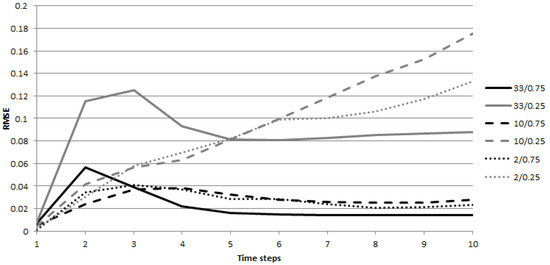
Figure 4.
RMSE at different time steps of the infection process for the fully observed scenario in the SIR model. The error is shown for observations at T.
Finally, from the optimization perspective, the task is moderately difficult for the FPSO algorithm. The performance varies depending on the task: the binary ones are easy, always taking less than two hundred iterations to conclude, while the real-valued scenarios with sparse infections are the most difficult, often requiring over a thousand iterations. The accuracy of the predictions is acceptable; for the majority of the test runs, the error remains below 5%, but there are cases where the search is less successful, for example, the 10/0.25 scenario for the IC model. Nonetheless, we can conclude that the optimization method performs well in this application.
4.4. Scalability
We close the evaluation by investigating the scalability of the optimization method. Our interests here are the average number of iterations the method requires to produce a solution, the total running time (a parallel version of the algorithm was implemented in C++, and the results were computed on a PC with a 4-core i7-4770 3.4 GHz processor) and the relationship between the size of the task and the accuracy of the estimation.
We examine four graphs in this section with nodes and 7753 edges and four infection scenarios from the previous section: 33% or 10% of the nodes are initially infected with an infection probability between 0 and 0.5 for the real-valued case and uniformly 1 for the binary case. Reference edge infection values were drawn from uniform random distributions between 0 and 0.25 and between 0 and 0.75. Both binary and real-valued two-observation infection scenarios were investigated. We only show results for the SIR model; the performance of the other models was similar. Each of these tasks was computed ten times and the results were averaged. The variance of the results was minimal.
Figure 5 shows the accuracy of the estimations, the average number of iterations and the running time for the above infection scenarios. The binary tasks remain much easier to solve than the real-valued tasks, requiring fewer iterations and less computational time to find a good estimation. The difference between the infection scenarios is also similar to that observed in the smaller examples, with larger infections being easier to predict. However, this depends on the ability of the graph to transfer infections (the reference edge values), as opposed to the fraction of initially infected vertices.
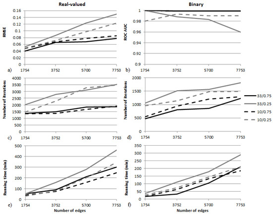
Figure 5.
Scalability results for the two-observation infection scenarios on four graphs. Both binary and real-valued cases are shown. RMSE and ROC AUC values can be seen in (a,b), the average number of iterations is shown in (c,d), and the average total running time in minutes is shown in (e,f).
Accuracy scaling can be seen in Figure 5a,b. The error of the estimation increases with the number of estimated values (edges), although the increase is significantly lower if the reference edge values are large. RMSE error values stay below 0.09 for all graphs if edge infections are large, but they are greater than 0.1 if infection values are small. Similar behavior can be observed in the binary case, where the classification is perfect if the transfer probabilities are large but remains below 1 if the edge values are small. The difference between scenarios with large and small edge infection probabilities can also be seen in Figure 5c,d, where the number of iterations required to find a good solution is much smaller if edge infection values are large. Finally, the running time of the tasks in minutes can be seen in Figure 5e,f. Depending on the size of the graph and the edge infection values, the tasks took one to eight hours on average to compute on the computer listed above.
Directly estimating the edge infection values in the GIIM is a difficult task, since the number of values to estimate, i.e., the number of edges, can be large, even for medium-sized graphs, posing a challenge for the optimization algorithm. In this section, we consider graphs with up to 4000 nodes and 7753 edges and show that estimation is possible on an average PC with acceptable accuracy and running time.
There are multiple ways to speed up the method so that it can handle large networks. The time complexity of the optimization depends heavily on the time complexity of the infection model. A modified version of the CompleteSim infection heuristic [28] was used in this study, but other potentially faster heuristics are available in the literature [12,28]. Another way to considerably speed up estimations is to assume that the edge infection values can be computed as functions of known vertex or edge attributes. In this case, only the coefficients of these functions have to be estimated, which are far less numerous than the number of edges in the graph.
5. Future Work
The scope of this study allowed us to test only part of the functionality provided by the Generalized Inverse Infection Model. However, there are many additional applications and extensions of the proposed model. Certain extensions are discussed below and will be explored in future work.
5.1. Time Scale of the Infection Process
So far, we have assumed that the sampling times of the reference and computed observations are the same: in , . This is usually not realistic, since many times, we cannot freely pick the exact moment that the observations are made or the number of observations. Real-life sampling times are continuous, for example, dates or clock time. Therefore, matching them to the sampling times of the simulated observation process may be non-trivial, especially if they are noisy as well. Additionally, infections in the real world might not behave the way that we expect them to. They can be influenced by factors unknown to the observer, suddenly become more virulent or stop for no apparent reason: the time scale of the infection process might be unknown. The relationship between the time scale of the observed and computed processes might not be linear or not even monotonic. Therefore, matching the observations on an artificially simulated infection process to real-life observations might be a difficult task.
5.2. Identifying and Calibrating the Infection Model
Another point of interest is the epidemic model. In some real-life applications, it is fairly possible that (1) the infection model is unknown or (2) the parameters of the infection model are unknown. In the first case, it might be worthwhile to start with a more general model and move to more specific ones. The second case is simpler: instead of looking for in , we are looking for or possibly both, where denotes the parameters of the infection function. If the edge weights are unknown, this might be a difficult task, since we are optimizing for both and .
6. Conclusions
In this paper, we explored some theoretical properties and demonstrated the general applicability of the Generalized Inverse Infection Model. Given an unweighted graph and a set of observations on an infection process, the GIIM is able to estimate the edge infection probabilities explaining the input observations. Contrary to existing models, our model is able to handle an arbitrary number of observations; it can be applied to fully, minimally or, potentially, partially observed infection processes. The nature of the observations is not fixed either; in the scope of this study, we experimented with binary and real node infection values, but it is possible to use other values tied to the spread of the infection process within the framework. The underlying infection model may also be customized: we worked with the SI, IC, SIR and SEIR models, but it is also possible to consider other network-based models. The GIIM formulates the inverse infection task as a general optimization problem, and a Particle Swarm Optimization method was suggested as the solution method. Finally, it is possible to further extend the functionality of the model, such as estimating the parameters of the infection model.
We evaluated the performance of the GIIM on a large variety of artificial infection scenarios. We have shown on trees that, even though the problem is underdetermined, it is possible to find accurate explanations of the infection process. In more general complex networks, we examined the behavior of our method on 108 different inverse infection tasks. Our findings indicate that there is a close relationship between the expected size of the infection and the difficulty of the task, with larger infections being easier to predict. There is a complex interplay between the density of initial infections, the likelihood of the infection spread and the difficulty of the estimation at different time steps. Finally, we experimented with larger networks and a few specific infection scenarios to investigate the scalability of the problem. We can say that the optimization method performs well for almost all of the situations described in this paper.
The GIIM method’s ability to predict edge infection values in real-life scenarios has already been proven in [24,25]. In this work, we have shown that the model’s flexibility and robustness allow it to be applied in wider settings than we have previously seen, paving the way for successful future applications of the model.
Author Contributions
Conceptualization, A.B. and L.G.; methodology, A.B and L.G.; software, A.B.; validation, A.B.; formal analysis, A.B. and L.G.; investigation, A.B. and L.G.; resources, A.B. and L.G.; data curation, A.B.; writing—original draft preparation, A.B. and L.G.; writing—review and editing, A.B. and L.G.; visualization, A.B.; supervision, A.B. and L.G.; project administration, L.G.; funding acquisition, L.G. All authors have read and agreed to the published version of the manuscript.
Funding
This research was funded by the National Health and Medical Research Council (NHMRC), grant number No. APP1082524.
Data Availability Statement
Data sharing not applicable.
Conflicts of Interest
The authors declare no conflict of interest.
Abbreviations
The following abbreviations are used in this manuscript:
| GIIM | Generalized Inverse Infection Model |
| SI | Susceptible Infected Model |
| SIR | Susceptible Infected Removed Model |
| SEIR | Susceptible Exposed Infected Removed Model |
| IC | Independent Cascade Model |
| RMSE | Root-Mean-Squared Error |
| ROC | Receiver Operator Characteristics |
| PSO | Particle Swarm Optimization |
| FPSO | Fully Informed Particle Swarm Optimization |
| IIP | Inverse Infection Problem |
| DAG | Directed Acyclic Graph |
References
- Andreson, R.M.; May, R.M.; Anderson, B. Infectious Diseases of Humans: Dynamics and Control; Oxford University Press: Oxford, UK, 1992. [Google Scholar]
- Diekmann, O.; Heesterbeek, J.A.P. Mathematical Epidemiology of Infectious Diseases. Model Building, Analysis and Interpretation; John Wiley & Sons: New York, NY, USA, 2000. [Google Scholar]
- Granovetter, M. Threshold models of collective behavior. Am. J. Sociol. 1978, 83, 1420–1443. [Google Scholar] [CrossRef]
- Bóta, A.; Csernenszky, A.; Győrffy, L.; Kovács, G.; Krész, M.; Pluhár, A. Applications of the Inverse Infection Problem on bank transaction networks. Cent. Eur. J. Oper. Res. 2015, 23, 345–356. [Google Scholar] [CrossRef]
- Csernenszky, A.; Kovács, G.; Krész, M.; Pluhár, A.; Tóth, T. The use of infection models in accounting and crediting. Chall. Anal. Econ. Bus. Soc. Prog. Szeged 2009, 617–623. [Google Scholar]
- Krész, M.; Pluhár, A. Economic Network Analysis based on Infection Models. In Encyclopedia of Social Network Analysis and Mining; Springer Science: New York, NY, USA, 2014; pp. 439–445. [Google Scholar]
- Domingos, P.; Richardson, M. Mining the Network Value of Costumers. In Proceedings of the 7th International Conference on Knowledge Discovery and Data Mining, San Francisco, CA, USA, 26–29 August 2001; pp. 57–66. [Google Scholar]
- Hajdu, L.; Krész, M.; Bóta, A. Community based influence maximization in the Independent Cascade Model. In Proceedings of the 2018 Federated Conference on Computer Science and Information Systems (FedCSIS), Poznań, Poland, 9–12 September 2018; pp. 237–243. [Google Scholar]
- Kempe, D.; Kleinberg, J.; Tardos, E. Maximizing the Spread of Influence though a Social Network. In Proceedings of the 9th ACM SIGKDD International Conference on Knowledge Discovery and Data Mining, Washington, DC, USA, 24–27 August 2003; pp. 137–146. [Google Scholar]
- Wang, X.; Zhang, Y.; Zhang, W.; Lin, X.; Chen, C. Bring Order into the Samples: A Novel Scalable Method for Influence Maximization. IEEE Trans. Knowl. Data Eng. 2016, 29, 243–256. [Google Scholar] [CrossRef]
- Du, N.; Song, L.; Smola, A.; Yuan, M. Learning networks of heterogeneous influence. Adv. Neural Inf. Process. Syst. 2012, 25, 2780–2788. [Google Scholar]
- Chen, W.; Yuan, Y.; Zhang, L. Scalable Influence Maximization in Social Networks under the Linear Threshold Model. In Proceedings of the ICDM ’10 Proceedings of the 2010 IEEE International Conference on Data Mining, Sydney, Australia, 13–17 December 2010; pp. 88–97. [Google Scholar]
- Gardner, L.; Fajardo, D.; Waller, S.T. Inferring Contagion Patterns in Social Contact Networks Using a Maximum Likelihood Approach. Nat. Hazards Rev. 2004, 15, 04014004. [Google Scholar] [CrossRef]
- Gardner, L.M.; Fajardo, D.; Waller, S.T. Inferring infection-spreading links in an air traffic network. Transp. Res. Rec. J. Transp. Res. Board 2012, 2300, 13–21. [Google Scholar] [CrossRef]
- Gardner, L.M.; Fajardo, D.; Waller, S.T.; Wang, O.; Sarkar, S. A Predictive Spatial Model to Quantify the Risk of Air-Travel-Associated Dengue Importation into the United States and Europe. J. Trop. Med. 2012, 2012, 103679. [Google Scholar] [CrossRef] [PubMed]
- Gomez-Rodriguez, M.; Leskovec, J.; Krause, A. Inferring networks of diffusion and influence. ACM Trans. Knowl. Discov. Data 2012, 5, 1–37. [Google Scholar] [CrossRef]
- Goyal, A.; Bonchi, F.; Lakshmanan, L.V.S. Learning influence probabilities in social networks. In Proceedings of the Third ACM International Conference on Web Search and Data Mining, New York, NY, USA, 3–6 February 2010; pp. 241–250. [Google Scholar]
- Kimura, M.; Saito, K. Tractable models for information diffusion in social networks. In Knowledge Discovery in Databases; Lecture Notes in Computer Science; Springer: Berlin/Heidelberg, Germany, 2006; pp. 259–271. [Google Scholar]
- Myers, S.; Leskovec, J. On the convexity of latent social network inference. Adv. Neural Inf. Process. Syst. 2010, 23, 1741–1749. [Google Scholar]
- Rey, D.; Gardner, L.; Waller, S.T. Finding Outbreak Trees in Networks with Limited Information. Netw. Spat. Econ. 2015, 16, 687–721. [Google Scholar] [CrossRef]
- Amin, K.; Heidari, H.; Kearns, M. Learning from contagion (without timestamps). In Proceedings of the 31st International Conference on Machine Learning (ICML-14), Beijing, China, 21–26 June 2014; pp. 1845–1853. [Google Scholar]
- Bóta, A.; Krész, M.; Pluhár, A. Systematic learning of edge probabilities in the Domingos-Richardson model. Int. J. Complex Syst. Sci. 2011, 1, 115–118. [Google Scholar]
- Bóta, A.; Krész, M.; Pluhár, A. The inverse infection problem. In Proceedings of the 2014 Federated Conference on Computer Science and Information Systems, Warsaw, Poland, 7–10 September 2014; pp. 75–83. [Google Scholar] [CrossRef]
- Bóta, A.; Holmberg, M.; Gardner, L.; Rosvall, M. Socioeconomic and environmental patterns behind H1N1 spreading in Sweden. Sci. Rep. 2021, 11, 22512. [Google Scholar] [CrossRef]
- Gardner, L.M.; Bóta, A.; Gangavarapu, A.; Kraemer, M.U. Inferring the risk factors behind the geographical spread and transmission of Zika in the Americas. PLoS Neglected Trop. Dis. 2018, 12, e0006194. [Google Scholar] [CrossRef]
- Kennedy, J.; Mendes, R. Neighborhood topologies in fully informed and best-of-neighborhood particle swarms. IEEE Trans. Syst. Man Cybern. Part C Appl. Rev. 2006, 36, 515–519. [Google Scholar] [CrossRef]
- Kennedy, J. Particle Swarm Optimization. In Encyclopedia of Machine Learning; Springer: New York, NY, USA, 2010; pp. 760–766. [Google Scholar]
- Bóta, A.; Krész, M.; Pluhár, A. Approximations of the Generalized Cascade Model. Acta Cybern. 2013, 21, 37–51. [Google Scholar] [CrossRef]
- Leskovec, J.; Kleinberg, J.; Faloutsos, C. Graphs over time: Densification laws, shrinking diameters and possible explanations. In Proceedings of the 1st ACM SIGKDD International Conference on Knowledge Discovery and Data Mining, Chicago, IL, USA, 21–24 August 2005; pp. 177–187. [Google Scholar]
Disclaimer/Publisher’s Note: The statements, opinions and data contained in all publications are solely those of the individual author(s) and contributor(s) and not of MDPI and/or the editor(s). MDPI and/or the editor(s) disclaim responsibility for any injury to people or property resulting from any ideas, methods, instructions or products referred to in the content. |
© 2023 by the authors. Licensee MDPI, Basel, Switzerland. This article is an open access article distributed under the terms and conditions of the Creative Commons Attribution (CC BY) license (https://creativecommons.org/licenses/by/4.0/).