Multiprocessor Fair Scheduling Based on an Improved Slime Mold Algorithm

Abstract

An improved slime mold algorithm (IMSMA) is presented in this paper for a multiprocessor multitask fair scheduling problem, which aims to reduce the average processing time. An initial population strategy based on Bernoulli mapping reverse learning is proposed for the slime mold algorithm. A Cauchy mutation strategy is employed to escape local optima, and the boundary-check mechanism of the slime mold swarm is optimized. The boundary conditions of the slime mold population are transformed into nonlinear, dynamically changing boundaries. This adjustment strengthens the slime mold algorithm’s global search capabilities in early iterations and strengthens its local search capability in later iterations, which accelerates the algorithm’s convergence speed. Two unimodal and two multimodal test functions from the CEC2019 benchmark are chosen for comparative experiments. The experiment results show the algorithm’s robust convergence and its capacity to escape local optima. The improved slime mold algorithm is applied to the multiprocessor fair scheduling problem to reduce the average execution time on each processor. Numerical experiments showed that the IMSMA performs better than other algorithms in terms of precision and convergence effectiveness.

1. Introduction

Multiprocessor systems are widely used in various fields, including medical systems, smartphones, aerospace, and more [1]. With the increasing demand for high performance and low power consumption in today’s society, the use of multiprocessor systems has been greatly promoted [2], leading to extensive research on task scheduling problems on multiprocessors. This paper investigates the problem of fair scheduling on multiprocessors, aiming to achieve a balanced average processing time across the processors when executing multiple independent nonpreemptive tasks. The motivation for this problem stems from a factory scenario, where there is a desire to allocate tasks to transportation vehicles in such a way that the average mileage for each vehicle is balanced. This model is also applicable to the fair scheduling problem of taxis, ensuring that the average distance covered by each taxi for deliveries is the same.

The fairness problem in scheduling was initially introduced by Fagin and Williams [3], who abstracted it as the carpool problem for their study. Subsequently, fairness scheduling problems started to emerge in the context of online machine scheduling. The goal of the scheduling problems is to minimize the maximum sum of processing time of the machines. In recent years, there has been an increasing focus on fairness in scheduling, particularly in the context of optimal real-time multiprocessor scheduling algorithms [4]. Research on proportionate fairness scheduling has long been conducted in the fields of operating systems, computer networks, and real-time systems [5]. The scheduling strategies for proportionate fairness are largely based on the concept of maintaining proportional progress rates among all tasks [6]. Due to its ability to balance system throughput and fairness, proportionate fairness scheduling has gained widespread adoption in practice [7].

Ensuring a fair allocation of resources can significantly impact the performance of scheduling algorithms. While various fair scheduling algorithms have been emerging rapidly, research on fair scheduling on multiprocessors is relatively limited. It has been established that the job scheduling problem for processors is NP-hard, and ensuring fairness in scheduling can improve the utilization of processor resources to some extent. The typical objective of fairness scheduling problems is usually to minimize the maximum total processing time on machines. This paper, however, sets the fairness scheduling objective as minimizing the average execution time on each processor.

Scheduling problems with the objective of minimizing the maximum average processing time can be applied to tasks such as taxi and courier dispatch, which require handling a large number of scheduling tasks in a short time, necessitating algorithms that are efficient and have short processing times. The fair scheduling issue for multiprocessor multitasking is addressed in this research using a modified slime mold method.

Swarm intelligence algorithms are mainly inspired by the evolution of organisms in the natural environment and the hunting, foraging, and survival processes of populations [8]. Some common swarm intelligence algorithms include particle swarm optimization (PSO) [9], the whale optimization algorithm (WOA) [10], the sparrow search algorithm (SSA) [11], the butterfly optimization algorithm (BOA) [12], and so on. These swarm intelligence algorithms have been studied and used extensively in a variety of fields, such as photovoltaic maximum power point tracking [13], multiobjective optimization problems [14], and COVID-19 infection prediction [15]. They have demonstrated good performance in solving problems in specific domains. A recently developed metaheuristic algorithm called the slime mold algorithm (SMA), which was introduced by Li et al. [16] in 2020, simulates the behavior and morphological changes of slime molds during natural foraging. Compared with other intelligent optimization algorithms, slime mold algorithm has the advantages of a simple principle, few adjustment parameters, a strong optimization ability, and an easy implementation.

The slime mold algorithm has been successfully applied in many fields, especially in engineering optimization. Premkumar et al. [14] proposed a multiobjective slime mold algorithm based on elite undominated ranking. They applied the slime mold algorithms to solving multiobjective optimization problems and proved that the proposed algorithm was effective in solving complex multiobjective problems. Gong et al. [17] proposed a hybrid algorithm based on a state-adaptive slime mold model and fractional order ant system (SSMFAS) to solve the traveling salesman problem (TSP). Experimental results showed that the algorithm had the competitiveness to find better solutions on TSP instances. By integrating chaos mapping and differing evolution strategies for overall optimization, Chen et al. [18] devised an enhanced slime mold algorithm, which was applied to engineering optimization problems. The whale optimization algorithm and the slime mold algorithm were combined by Abdel-Basset et al. [19] to tackle a chest X-ray separation of images issue. Gush et al. [20] used slime mold algorithms to optimize the optimal intelligent inverter control system of photovoltaic and energy storage systems to improve the photovoltaic carrying capacity of the distribution network.

In this paper, an improved slime mold algorithm is considered to study the fair scheduling of multiprocessor and multitasking. Through in-depth research on slime mold algorithms, it was found that there were still certain limitations. For example, the population diversity is not rich enough, the convergence speed is slow, and it is easy to fall into a local optimal solution. In the standard iteration process of the SMA, the random initialization of the slime mold swarm reduces the potential for population diversity. It also lacks effective solutions when addressing population converged to local optima. The fixed boundary check strategy in the standard SMA makes it difficult to return to the better positions when slime molds exceed the boundaries. This paper makes multistrategy improvements to the standard slime mold algorithm.

The main contributions of this paper are as follows:

• A reverse learning initialization population strategy based on Bernoulli chaotic mapping is introduced to increase the diversity of populations.
• Cauchy mutations are introduced to help slime mold populations jump out of a local optimal solution.
• A nonlinear dynamic boundary improvement strategy is introduced to accelerate the convergence rate of the population.
• The IMSMA is applied to solving the fair scheduling problem on multiprocessors to minimize the average processing time on each processor.

The article organization is as follows. Section 1 introduces the research about fair scheduling problems and the slime mold algorithm. Section 2 describes some relevant literature on fair scheduling. The conventional slime mold algorithm is presented in Section 3. Section 4 provides detailed improvement strategies for the improved slime mold algorithm (IMSMA). The simulation tests are presented in Section 5. Section 6 models the fair scheduling problem on multiprocessors and applies the IMSMA to solve it. Section 7 provides numerical experiments for fair scheduling on multiple processors. Conclusions are given in Section 8.

2. Related Work

Guaranteeing the fair distribution of resources can have a notable influence on the effectiveness of scheduling algorithms. In the realm of scheduling problems, fairness can be defined in various ways. There exists a wealth of literature dedicated to defining fairness concepts and designing efficient algorithms with fair constraints [21]. Zhong et al. [22] addressed the fair scheduling problem of multicloud workflow tasks and proposed a reinforcement learning-based algorithm. In response to cache contention issues in on-chip multiprocessors, a thread cooperative scheduling technique considering fairness was proposed by Xiao et al. [23]. It was based on non-cooperative game theory. They wanted to ensure equitable thread scheduling in order to improve the performance of the entire system. On heterogeneous processors with multiple cores, Salami et al. [24] suggested an energy-efficient framework for addressing fairness-aware schedules. This framework simultaneously addressed fairness and efficiency issues in multicore processors. For multiprocess contexts, Mohtasham et al. [25] developed a fair resource distribution method that aimed to maximize the overall system utility and fairness. This technique enabled the concurrent execution of multiple scalable processes even under CPU load constraints. Jung et al. [26] presented a multiprocessor-system fair scheduling algorithm based on task satisfaction metrics, which achieved a high proportion of fairness even under highly skewed weight distributions. Their algorithm quantified and evaluated fairness using service-time errors. A review of pertinent research on fair scheduling is given in

Table 1. Research on fair scheduling in the relevant literature.

Zhong et al. [22]	To optimize the scheduling order for multiple workflow tasks, they designed a reinforcement learning-based fair scheduling algorithm for multiworkflow tasks.	The authors created an evolving priority-driven method to avoid service level agreement violations through dynamic scheduling. Additionally, they implemented load balancing between virtual machines using a reinforcement learning algorithm.
Xiao et al. [23]	They proposed a fairness-aware thread collaborative scheduling algorithm based on uncooperative game theory, and the on-chip multiprocessor cache congestion problem was addressed.	The authors aimed to enhance the overall system performance by fairly scheduling threads. They employed an uncooperative game approach to address the thread collaborative schedule problem and introduced an iterative algorithm for finding the Nash equilibrium in non-cooperative games. This allowed them to obtain a collaborative scheduling solution for all threads.
Salami et al. [24]	Specifically addressing the different multicore processors’ fair energy-effective schedule dilemma, they proposed an energy-efficient framework that took into account fairness in a heterogeneous context.	Dynamic voltage and frequency scaling was used in the authors’ suggested energy-effective framework with a heterogeneous fairness awareness in order to satisfy fairness restrictions and offer an efficient energy-effective schedule. In comparison to the Linux regular scheduler, experimental results showed a significant improvement in both efficiency of energy and fairness.
Mohtasham et al. [25]	The authors proposed a fair distribution of resources method for a multiprocess context aimed at maximizing overall system utility and fairness.	The allocation of resources issue was first formalized as an NP-hard issue. Then, in pseudo-polynomial time, they employed approximation strategies and the convex optimization theory to identify the best answer to the posed problem. This fair resource allocation technique could run multiple scalable processes under CPU load constraints.
Jung et al. [26]	They proposed a multiprocessor-system fair scheduling algorithm based on task satisfaction metrics.	Their algorithm quantified and evaluated fairness using service time errors. It achieved a high proportion of fairness even under highly skewed weight distributions.

.

3. Standard Slime Mold Algorithm (SMA)

The slime mold algorithm was inspired by the foraging behavior of multicephalic velvet fungus, and the corresponding mathematical model was established. There are three phases: approaching food, surrounding food, and grabbing food [16]. In the stage of approaching food, the slime mold is spontaneously approaching food according to the smell in the environment. The expansion law can be expressed by the formula:

$$X\left(t+1\right)=\left\{\begin{array}{c}{X}_b\left(t\right)+vb\times \left(W\times X_A\left(t\right)-X_B\left(t\right)\right),r_1<p\hfill \\ vc\times X\left(t\right),r_1\ge p\hfill \end{array}\right.$$

(1)

where $X\left(t+1\right)$ and $X\left(t\right)$ indicate the position of slime molds at the $(t+1)$th and tth iterations, respectively. The operation "×" represents multiplication. $X_b\left(t\right)$ represents the fittest location of the slime molds in terms of fitness from the beginning to the current iteration. $X_A\left(t\right)$ and $X_B\left(t\right)$ stand for two random positions of the slime mold in the population chosen randomly. $r_1$ is a random number between zero and one. $vb$ is an arbitrary quantity within $[-a,a]$, where the variation of $vb$ simulates the slime mold’s choice between approaching food or continuing the search. $vc$ is the oscillation vector of the slime mold, which modifies its search trajectory. It ranges linearly from one to zero. The parameter a and the selection probability p are determined as follows:

$$a=arctan\mathrm{h}\left(1-t/T\right)$$

(2)

$$p=tan\mathrm{h}\left(\left|S\left(i\right)-DF\right|\right)$$

(3)

The population size of slime molds is expressed by the number $i=1,2,\dots ,N$. t embodies the current iteration number, and T is the maximum number of iterations. $S\left(i\right)$ symbolizes the fitness score of the ith slime mold, and $DF$ stands for the best fitness score obtained throughout all iterations.

The following is the weight W’s updating formula:

$$W\left(IndexSorted\left(i\right)\right)\left\{\begin{array}{c}1+r_2\times log\frac{bF-S\left(i\right)}{bF-wF}+1,i=condition\hfill \\ 1-r_2\times log\frac{bF-S\left(i\right)}{bF-wF}+1,i=others\hfill \end{array}\right.$$

(4)

$$IndexSorted=sort\left(S\right)$$

(5)

where $condition$ represents slime mold individuals with the top half of fitness values; and $others$ represents the remaining individuals. $r_1$ is a random number between zero and one. $bF$ and $wF$ represent the best and worst fitness scores of the present iteration, respectively. The operation "×" represents multiplication. The logarithm function is applied in the formula to slow down the rate of numerical changes caused by the contraction of the slime mold, stabilizing the frequency of contraction. $Condition$ simulates the process where the slime mold alters its location based on the quantity of food, with higher food concentrations leading to higher weights for slime molds in the vicinity. The sorted list of fitness values is expressed by $IndexSorted$.

During the course of looking for food, slime mold individuals separate a portion of the population to discover new territory and attempt to discover better quality solutions. This increases the possibilities of solution. The position update formula for the slime mold algorithm is expressed by:

$$X\left(t+1\right)=\left\{\begin{array}{c}rand\times \left(ub-lb\right)+lb,rand<z\hfill \\ X_b\left(t\right)+vb\times \left(W\times X_A\left(t\right)-X_B\left(t\right)\right),rand\ge z,r_1<p\hfill \\ vc\times X\left(t\right),rand\ge z,r_1\ge p\hfill \end{array}\right.$$

(6)

where $rand$ represents a random number between zero and one; $ub$ and $lb$ represent the lower and upper boundaries of the searching area. The operation "×" represents multiplication, and z represents the probability of slime mold individuals separating from the population to search for alternative food sources. Typically, z is set to $0.03$.

4. Improved Slime Mold Algorithm (IMSMA)

4.1. Population Initialization Strategy Based on Bernoulli Mapping and Reverse Learning

The effectiveness of an algorithm is greatly influenced by the population initialization. Chaotic mapping methods possess the characteristics of traversing and randomness, which are appropriate for early-stage exploration of possible regions and can increase the algorithm’s variety [18]. Common chaotic mapping models include tent mapping [27] and logistics mapping [28]. Compared to them, Bernoulli mapping [29] exhibits a more uniform distribution. Therefore, this study incorporated Bernoulli chaotic mapping into the population’s initialization method in of the slime mold algorithm. The equation is

$$y_{k+1}=\left\{\begin{array}{c}{y}_k/\left(1-\lambda \right),y_k\in \left(0,1-\lambda \right]\hfill \\ \left(y_k-1+\lambda \right)/\lambda ,y_k\in \left(1-\lambda ,1\right)\hfill \end{array}\right.$$

(7)

$$X=lb+\left(ub-lb\right)\times y.$$

(8)

In Equation (7), k stands for the times of chaotic iterations, and $\lambda$ is the chaotic mapping’s parameter, typically set to $0.4$. The generated chaotic sequence y is mapped to the search space of solutions, as shown in Equation (8). Here, X represents the value mapped within the solution interval $lb$ and $ub$ are the slime mold’s boundaries. The operation "×" represents multiplication.

In addition, the opposite learning approach adopts the idea of obtaining reverse solutions from the initial population. By adding reverse solutions, it is possible to further boost population variety [30], enhancing the search capability of the algorithm. Therefore, in this study, after applying the Bernoulli mapping to the population, the opposite learning approach was employed. The opposite learning approach is an improvement approach proposed by Tizhoosh in the field of swarm intelligence in 2005 [31]. Its concept is to generate a reverse solution based on the current solution in the course of the optimization procedure. In order to choose the best solution for the subsequent iteration, the objective function values of the present solution and the opposite solution are compared. The following is the formula for producing the opposite solution:

$$X^{*}=lb+ub-X.$$

(9)

In Equation (9), $X^{*}$ denotes the reverse solution of the slime mold population, $lb$ and $ub$ are the highest and lowest boundaries of the searching space for the slime mold population, and X represents the current solution of the slime mold population. The obtained reverse solution is then merged with the original solution to form a new population $X=(X^{*}\cup X)$. According to their objective function values, the new population’s fitness values are computed. Subsequently, the fitness values are sorted, and the first half of the population is selected as the initial population.

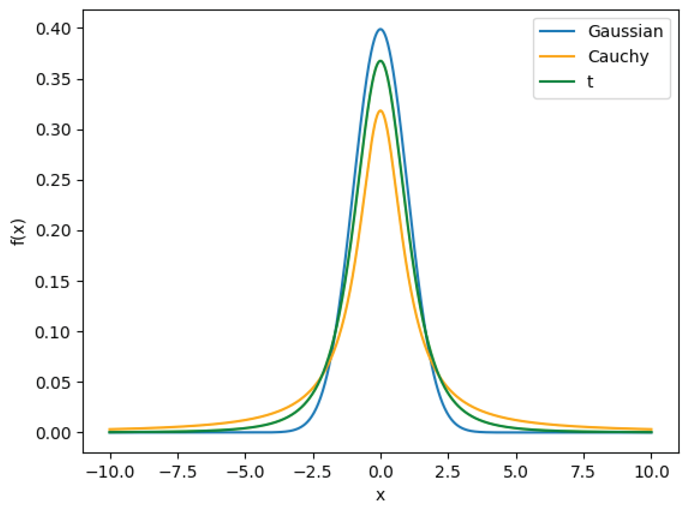
4.2. Cauchy Mutation Strategy for Escaping Local Optima

The Cauchy distribution is where the Cauchy mutation comes from [32]. The following describes the standard Cauchy distribution’s probability density function:

$$f\left(x\right)=\frac{1}{\pi }·\frac{1}{1+x^2},x\in \left(-\infty ,\infty \right).$$

(10)

Figure 1 illustrates the probability density function curved lines of the standard Gaussian distribution, the standard Cauchy distribution, and the standard t-distribution. Through an analysis of the curves, it can be observed that comparing the Gaussian and t-distributions to the Cauchy distribution reveals that it is broader and flatter, and it approaches zero more slowly. Additionally, in comparison to the Gaussian and t-distributions, the Cauchy distribution’s origin peak is smaller. This smaller peak guides individuals to use a lesser time trying to find the optimal position [33]. Therefore, the Cauchy mutation exhibits a stronger perturbation and is more conducive to helping the slime mold population escape local optima.

The update strategy for the current best solution is as follows:

$$X_{ij}^{new}=X_{ij}+cauchy\left(0,1\right)·X_{ij}.$$

(11)

In Equation (11), $cauchy(0,1)$ represents the common Cauchy distribution. The Cauchy distribution’s randomly generating function is written as $\eta =tan\left(\pi ·\left(\xi -0.5\right)\right)$, where $\xi$ indicates a randomly vector ranging from 0 to 1. $x_{ij}$ symbolizes the location of the ith individual at the jth dimension, and $x_{ij}^{new}$ stands for the fresh location of the ith individual at the jth dimension after undergoing a Cauchy mutation.

If the population’s global best solution has not been updated for more than 5 iterations throughout the iterative updating procedure of the slime mold algorithm, it is considered that the population may be stuck in its local optimum. In order to boost the likelihood of escape the regional optimal, a Cauchy mutation is applied. The condition for defining that the population’s global best value was not updated is that the absolute difference between the fitness value $f_{best}^t$ obtained from the current iteration’s best position and the global best value $f_{Gbest}$ is less than $\Delta$, as shown in the following equation:

$$\Delta \ge \left|f_{best}^t-f_{Gbest}\right|$$

(12)

where t is the current iteration number, and by definition, when $\Delta$ = 0.001, the algorithm is stuck at a local optimum. In this instance, the slime mold population utilizes the Cauchy mutation to assist it in eluding the local optimum.

4.3. Nonlinear Dynamic Boundary Conditions

The traditional SMA often experiences the issue of slime mold positions exceeding the boundaries during the early iterations. The typical approach for handling boundary conditions is to set the value of individuals exceeding the top edge to the top border value, and set the value of individuals exceeding the lower border to the lower border value. However, this boundary condition handling method is not conducive to algorithm convergence [13]. In this study, we propose a nonlinear dynamic boundary condition, as shown in the following equation:

$$X_{ij}\left(t\right)=\left\{\begin{array}{c}{X}_{ij}^{rand}\left(t\right)+c_1·k\left(ub-X_{ij}^{rand}\left(t\right)\right),X_{ij}\left(t\right)>ub\hfill \\ X_{ij}^{rand}\left(t\right)-c_2·k\left(X_{ij}^{rand}\left(t\right)-lb\right),X_{ij}\left(t\right)\le lb\hfill \end{array}\right.$$

(13)

$$k=k_1{\left(\frac{T-t}{T}\right)}^{k_2\frac{t}{T}}$$

(14)

where $X_{ij}^{rand}\left(t\right)$ represents a random slime mold position; $c_1$ and $c_2$ are two random numbers between 0 and 1; $k_1$ and $k_2$ are amplitude adjustment coefficients that control the magnitude of parameter k, with $k_1$ and $k_2$ set to 1.5 and 5, respectively. During the early iterations when the slime mold positions are far from the global optimum, the value of k decreases slowly. Slime molds that exceed the position range are greatly influenced by the coefficient k, enhancing the slime mold algorithm’s capability to search globally. During the later iterations, the slime mold positions are less affected by the value of k and more influenced by the best position, leading to a stronger local search capability and quicker algorithm convergence rate.

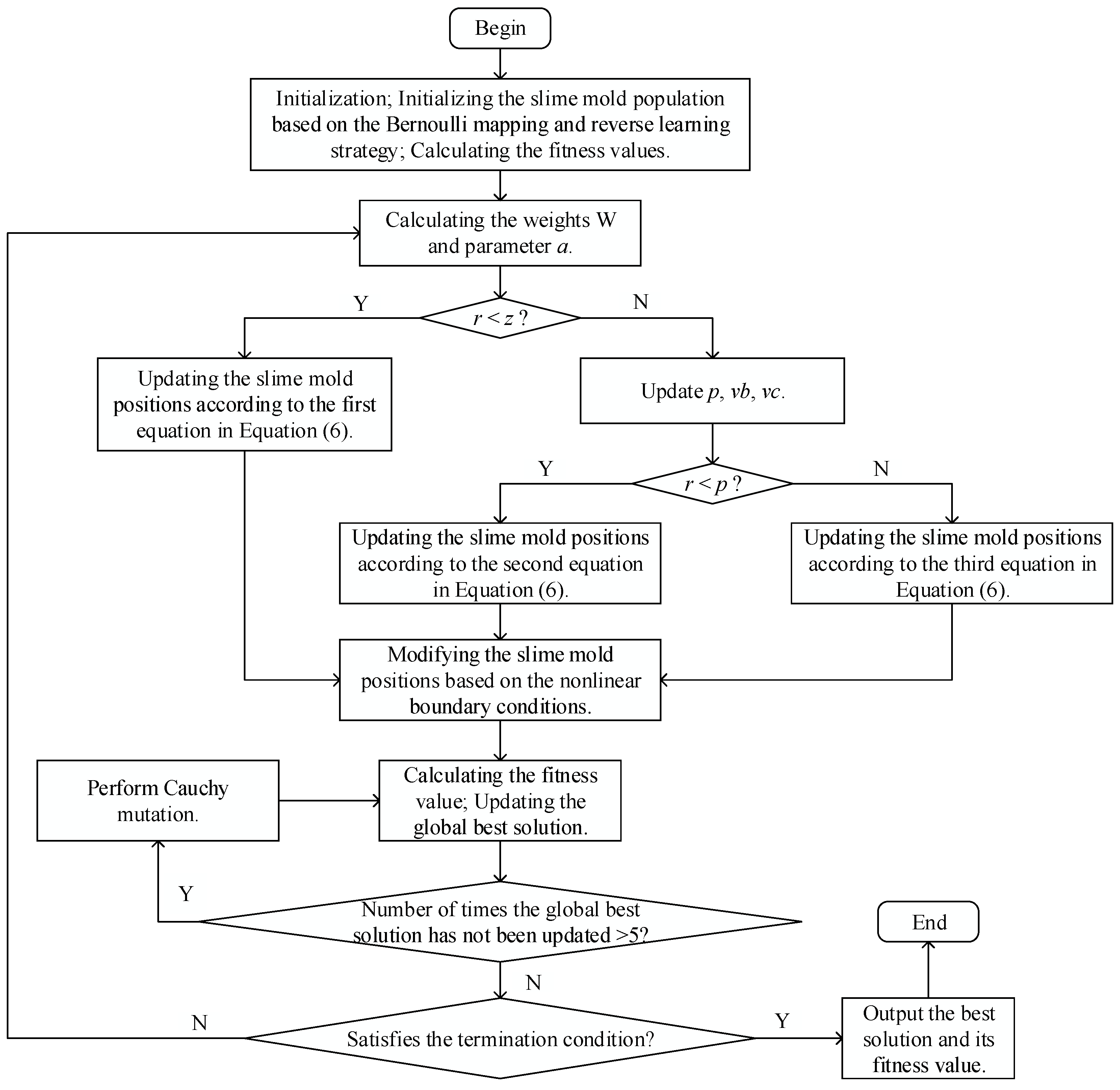
4.4. IMSMA Flowchart and Pseudocode

The flowchart of the improved slime mold algorithm (IMSMA) is shown in Figure 2.

First, the initialization of the slime mold population is performed using the direction learning strategy based on the Bernoulli map. Subsequently, the weights (W) of the slime molds and the value of parameter a are calculated. Random number r is compared to parameter z. If r is less than z, the slime mold positions are updated using the first equation in Equation (6). If r is greater than or equal to z, the values of parameters p, $vb$, and $vc$ are updated, and then r is compared to p. If r is less than p, the slime mold positions are updated using the second equation in Equation (6). If r is greater than or equal to p, the slime mold positions are updated using the third equation in Equation (6). Next, nonlinear boundary conditions are applied to modify the positions of the slime molds. The fitness values of the slime molds are calculated, and the global optimal value is updated. It is then checked whether the global optimal value has not been updated for more than five times. If it has, it is considered that the algorithm has converged to a global optimal value. In this case, the Cauchy mutation strategy is applied to update the positions, and the global optimal value is recalculated and updated. If the global optimal value has changed at least once within a continuous span of 5 times, it is checked whether the termination condition is met. If the condition is not met, the iteration continues. If the condition is met, the algorithm terminates, and the optimal solution and the optimal fitness value are outputted.

The pseudocode for the improved slime mold algorithm (IMSMA) is as follows:

Step 1.

Initialization: T, $Dim$, slime mold population N, z, $lb$, $ub$.

Step 2.

Based on the Bernoulli mapping reverse learning strategy, initialize the positions of the slime mold population. Do the fitness calculations and rank them in order to find the best fitness value $bF$ and the poorest fitness value $wF$.

Step 3.

Calculate the values of the weight W and the parameter a.

Step 4.

If rand < z: on the basis of the first equation in Equation (6), adjust the locations of the slime molds; go to step 6.

Else: update p, $vb$, $vc$; go to step 5.

Step 5.

If r < p: on the basis of the second equation in Equation (6), adjust the locations of the slime molds; go to step 6.

Else: on the basis of the third equation in Equation (6), adjust the locations of the slime molds; go to step 6.

Step 6.

Revise the locations of the slime molds based on the nonlinear dynamic boundary conditions. Update the global optimal solution after calculating the fitness values.

Step 7.

If the global best solution has not changed more than five times, perform a Cauchy mutation on the positions of the slime molds; go to step 6.

Step 8.

If the termination condition is not satisfied, go to step 3.

Else: generate the best answer and its fitness value, and terminate the program.

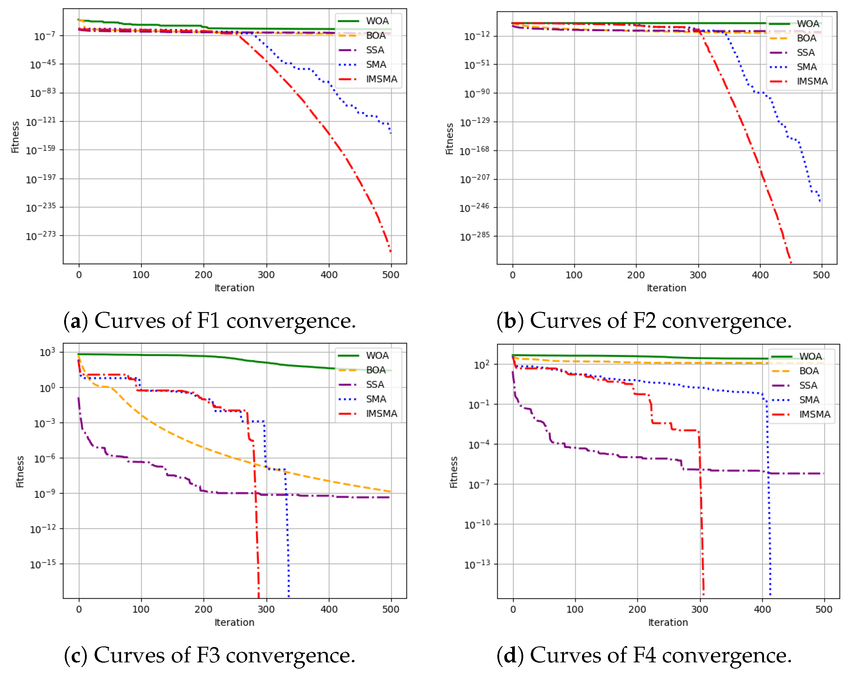
5. Performance Testing and Analysis of the Improved Slime Mold Algorithm

To test the performance of the improved slime mold algorithm, simulation experiments were conducted. The experimental environment utilized an 11th Gen Intel^® Core^TM i5-11400H CPU with a clock speed of 2.70 GHz (Intel Corporation, Santa Clara, CA, USA), 16 GB of RAM, and a 64-bit Windows 11 operating system. The programming language used was Python, version 3.6. Four test functions, namely F1 to F4, were selected for the experiments. F1 and F2 are unimodal functions, while F3 and F4 are multimodal functions from the CEC2019 benchmark test functions. Detailed information about these four benchmark test functions is provided in

Table 2. Benchmark test functions details.

Function	Function Expressions	Number of Peaks	Variable Range
F1	$f_1\left(x\right)={\sum }_{i=1}^n\left|x_i\right|+{\prod }_{i=1}^n\left|x_i\right|$	Unimodal	[−10, 10]
F2	$f_2\left(x\right)={\sum }_{i=1}^n{\left({\sum }_{j=1}^i{x}_j\right)}^2$	Unimodal	[−100, 100]
F3	$f_3\left(x\right)=\frac{1}{4000}{\sum }_{i=1}^n{x}_i^2-{\prod }_{i=1}^{n}cos\left(\frac{x_i}{\sqrt{i}}\right)+1$	Multimodal	[−600, 600]
F4	$f_4={\sum }_{i=1}^n\left(x_i^2-10cos\left(2\pi x_i\right)+10\right)$	Multimodal	[−5.12, 5.12]

.

The algorithm’s performance was assessed using the four chosen test functions, and a comparison was made among the WOA, BOA, SSA, SMA, and the IMSMA proposed in this paper. To ensure fairness in the experiments, the testing environment and algorithm parameters were set to the same values. The swarm size was fixed at 30 for all intelligent algorithms, with a dimension of 30 and a maximum iteration of 500. The convergence curved lines of the five algorithms are displayed in Figure 3 after each benchmark function was executed 30 times.

The specific test results of the five algorithms are shown in

Table 3. Comparison table of algorithms’ test results.

Function	Algorithms	Average Fitness Value	Standard Deviation	Best Value	Worst Value
F1	WOA	8.5850 $\times {10}^0$	5.3670 $\times {10}^0$	1.3076 $\times {10}^0$	2.2033 $\times {10}^1$
	BOA	1.2247 $\times {10}^{-6}$	4.0456 $\times {10}^{-7}$	3.7431 $\times {10}^{-7}$	2.1905 $\times {10}^{-6}$
	SSA	4.1472 $\times {10}^{-5}$	0.0002 $\times {10}^0$	1.5931 $\times {10}^{-96}$	0.0010 $\times {10}^0$
	SMA	3.2471 $\times {10}^{-138}$	1.7486 $\times {10}^{-137}$	2.9324 $\times {10}^{-278}$	9.7413 $\times {10}^{-137}$
	IMSMA	1.1214 $\times {\mathbf{10}}^{-\mathbf{295}}$	0.0000 $\times {\mathbf{10}}^{\mathbf{0}}$	0.0000 $\times {\mathbf{10}}^{\mathbf{0}}$	3.3642 $\times {\mathbf{10}}^{-\mathbf{294}}$
F2	WOA	9.2021 $\times {10}^4$	2.6686 $\times {10}^4$	4.9993 $\times {10}^4$	1.4113 $\times {10}^5$
	BOA	5.5098 $\times {10}^{-10}$	3.9426 $\times {10}^{-11}$	4.7340 $\times {10}^{-10}$	6.3100 $\times {10}^{-10}$
	SSA	8.0274 $\times {10}^{-8}$	3.2021 $\times {10}^{-7}$	0.0000 $\times {\mathbf{10}}^{\mathbf{0}}$	1.7711 $\times {10}^{-6}$
	SMA	5.3711 $\times {10}^{-241}$	0.0000 $\times {\mathbf{10}}^{\mathbf{0}}$	0.0000 $\times {\mathbf{10}}^{\mathbf{0}}$	1.6113 $\times {10}^{-239}$
	IMSMA	0.0000 $\times {\mathbf{10}}^{\mathbf{0}}$	0.0000 $\times {\mathbf{10}}^{\mathbf{0}}$	0.0000 $\times {\mathbf{10}}^{\mathbf{0}}$	0.0000 $\times {\mathbf{10}}^{\mathbf{0}}$
F3	WOA	2.5141 $\times {10}^1$	2.5713 $\times {10}^1$	1.5288 $\times {10}^0$	1.0146 $\times {10}^2$
	BOA	1.2962 $\times {10}^{-9}$	2.4117 $\times {10}^{-10}$	9.6035 $\times {10}^{-10}$	2.0675 $\times {10}^{-9}$
	SSA	4.2729 $\times {10}^{-10}$	1.5760 $\times {10}^{-10}$	0.0000 $\times {\mathbf{10}}^{\mathbf{0}}$	7.3477 $\times {10}^{-9}$
	SMA	0.0000 $\times {\mathbf{10}}^{\mathbf{0}}$	0.0000 $\times {\mathbf{10}}^{\mathbf{0}}$	0.0000 $\times {\mathbf{10}}^{\mathbf{0}}$	0.0000 $\times {\mathbf{10}}^{\mathbf{0}}$
	IMSMA	0.0000 $\times {\mathbf{10}}^{\mathbf{0}}$	0.0000 $\times {\mathbf{10}}^{\mathbf{0}}$	0.0000 $\times {\mathbf{10}}^{\mathbf{0}}$	0.0000 $\times {\mathbf{10}}^{\mathbf{0}}$
F4	WOA	2.4084 $\times {10}^2$	8.0646 $\times {10}^1$	6.5122 $\times {10}^1$	3.4340 $\times {10}^2$
	BOA	1.1291 $\times {10}^2$	8.6531 $\times {10}^1$	8.1465 $\times {10}^{-9}$	2.0361 $\times {10}^2$
	SSA	5.8915 $\times {10}^{-7}$	2.5701 $\times {10}^{-6}$	0.0000 $\times {\mathbf{10}}^{\mathbf{0}}$	1.4265 $\times {10}^{-5}$
	SMA	0.0000 $\times {\mathbf{10}}^{\mathbf{0}}$	0.0000 $\times {\mathbf{10}}^{\mathbf{0}}$	0.0000 $\times {\mathbf{10}}^{\mathbf{0}}$	0.0000 $\times {\mathbf{10}}^{\mathbf{0}}$
	IMSMA	0.0000 $\times {\mathbf{10}}^{\mathbf{0}}$	0.0000 $\times {\mathbf{10}}^{\mathbf{0}}$	0.0000 $\times {\mathbf{10}}^{\mathbf{0}}$	0.0000 $\times {\mathbf{10}}^{\mathbf{0}}$

.

Analyzing the experimental results and the convergence curves of algorithms, for function F1, from its convergence curve, it can be observed that the IMSMA starts to converge around 260 iterations, while SMA starts to converge around 280 iterations. The IMSMA exhibits a slightly faster convergence speed. From the final results of 30 experiments, the IMSMA achieves an average fitness value of 1.1214 $\times {10}^{-295}$, as can be observed, which is even closer to the theoretical optimum value of 0. For function F2, the IMSMA starts to converge around 300 iterations, and it exhibits the fastest convergence speed. From Table 3, it is evident that the IMSMA obtains a fitness value of zero on average, indicating that it can find the optimal result. For function F3, the convergence curve plot shows that the SSA and BOA have better convergence performance than the IMSMA in the first 300 iterations. However, after 300 iterations, the SSA gets trapped in local optima and struggles to escape, while BOA’s convergence curve becomes flatter, resulting in a slower convergence speed. On the other hand, the IMSMA and SMA quickly converge and find the optimal value around 300 iterations. Comparing the IMSMA and SMA individually, it can be observed that the IMSMA rapidly converges at around 270 iterations and finds the optimal value of zero, while SMA converges faster at around 330 iterations. Table 3 also shows that the IMSMA has an average fitness value, best value, and worst value of zero, indicating that the IMSMA outperforms the SMA. For function F4, the early versions of the SSA provide the best convergence performance, as can be seen from the graphic of the convergence curves. However, in subsequent iterations, its convergence speed becomes significantly slower. On the other hand, the IMSMA shows a good ability to escape local optima between the 200th and 300th iterations, and it reaches the ideal value after only 300 iterations. The SMA converges to the optimal value at around 410 iterations. Through testing the algorithms on the four functions, it can be concluded that the WOA performs the worst and exhibits a convergence stagnation. The IMSMA achieves the best performance with the fastest convergence speed and a good ability to escape local optima.

6. Solving Multiprocessor Fair Scheduling Problem with IMSMA

6.1. Establishment of the Multiprocessor Fair Scheduling Problem Model

The task scheduling problem on multiprocessors has been proven to be an NP-hard problem. Ensuring fairness in scheduling can improve the utilization of processor resources to some extent. Depending on different application scenarios, the definition of fairness may vary. To accomplish fair scheduling, we focused on the average process time on each processor and aimed to minimize the maximum average execution time on each processor to achieve fair scheduling. We established a model for the multiprocessor fair scheduling problem based on this objective. Assuming n jobs and m processors, let $P_{ij}$ represent the time required for job i to be executed on processor j. We introduce a binary variable $x_{ij}$ to indicate whether job i is run on processor j or not. The formulation is as follows:

$$x_{ij}=\left\{\begin{array}{c}1,condition\hfill \\ 0,other\hfill \end{array}\right..$$

(15)

The $condition$ represents the case where job i is run on processor j, and $other$ represents all other cases. One processor can handle only one task at a time, so the constraint conditions are as follows:

$$\sum _{j=1}^m{x}_{ij}=1,i=1\cdots n.$$

(16)

Assuming the total execution time on each processor is P, we have the following constraint:

$$P_j=\sum _{i=1}^n{P}_{ij}{x}_{ij},j=1\cdots m.$$

(17)

The average execution time on each processor $P_j^{avg}$ is represented as follows:

$$P_j^{avg}=\frac{P_j}{{\sum }_{i=1}^n{x}_{ij}},j=1\cdots m.$$

(18)

The following is a representation of the objective function:

$$F\left(x\right)=min\left(max\left\{P_1^{avg},P_2^{avg},P_3^{avg},\cdots ,P_m^{avg}\right\}\right)$$

(19)

$$s.t.=\left\{\begin{array}{c}\left(15\right)\hfill \\ \left(16\right)\hfill \\ \left(17\right)\hfill \\ \left(18\right)\hfill \end{array}\right.$$

(20)

The objective function is constrained by Equations (15)–(18). To facilitate solving the equation, let us consider the continuous approximation of the discrete objective function:

$$F\left(x\right)=min\left(P_1^{avg}+P_2^{avg}+\cdots +P_m^{avg}\right)+{\mu }_1\sum _{i=1}^n\left(x_{i1}+x_{i2}+\cdots +x_{im}-1\right)+{\mu }_2\sum _{i=1}^n\sum _{j=1}^m\left(x_{ij}-x_{ij}^2\right).$$

(21)

In the equation, ${\mu }_1$ and ${\mu }_2$ are two random numbers between zero and one. The two additional terms added afterwards are introduced to represent that $x_{ij}$ is a binary variable.

6.2. Description of Multiprocessor Fair Scheduling Algorithm Based on IMSMA

Suppose a system with n tasks and m processors. When initializing the slime mold population, it is important to set the dimension of the slime mold swarm size to $n\times m$. The description of the IMSMA for multiprocessor fair scheduling is as follows:

Step 1.

Initialization: T, $Dim$, slime mold population N, z, $lb$, $ub$, n, m.

Step 2.

Based on the Bernoulli mapping reverse learning strategy, initialize the positions of the slime mold population.

Step 3.

Input the objective function for multiprocessor fair scheduling. Calculate the fitness values and sort them to obtain the greatest fitness value $bF$ and the poorest fitness value $wF$.

Step 4.

Calculate the values of the weight W and the parameter a.

Step 5.

If rand < z: on the basis of the first equation in Equation (6), adjust the locations of the slime molds; go to step 7.

Else: update p, $vb$, $vc$; go to step 6.

Step 6.

If r < p: on the basis of the second equation in Equation (6), adjust the locations of the slime molds; go to step 7.

Else: determine the location of the slime molds using the third equation in Equation (6); go to step 7.

Step 7.

Revise the locations of the slime molds based on the nonlinear dynamic boundary conditions. Update the global optimal solution after calculating the fitness values.

Step 8.

If the global best solution has not been changed more than five times, perform Cauchy mutation on the positions of the slime molds; go to step 7.

Step 9.

If the termination condition is not satisfied, go to step 4;

Else: generate the best answer and its fitness value, and terminate the program.

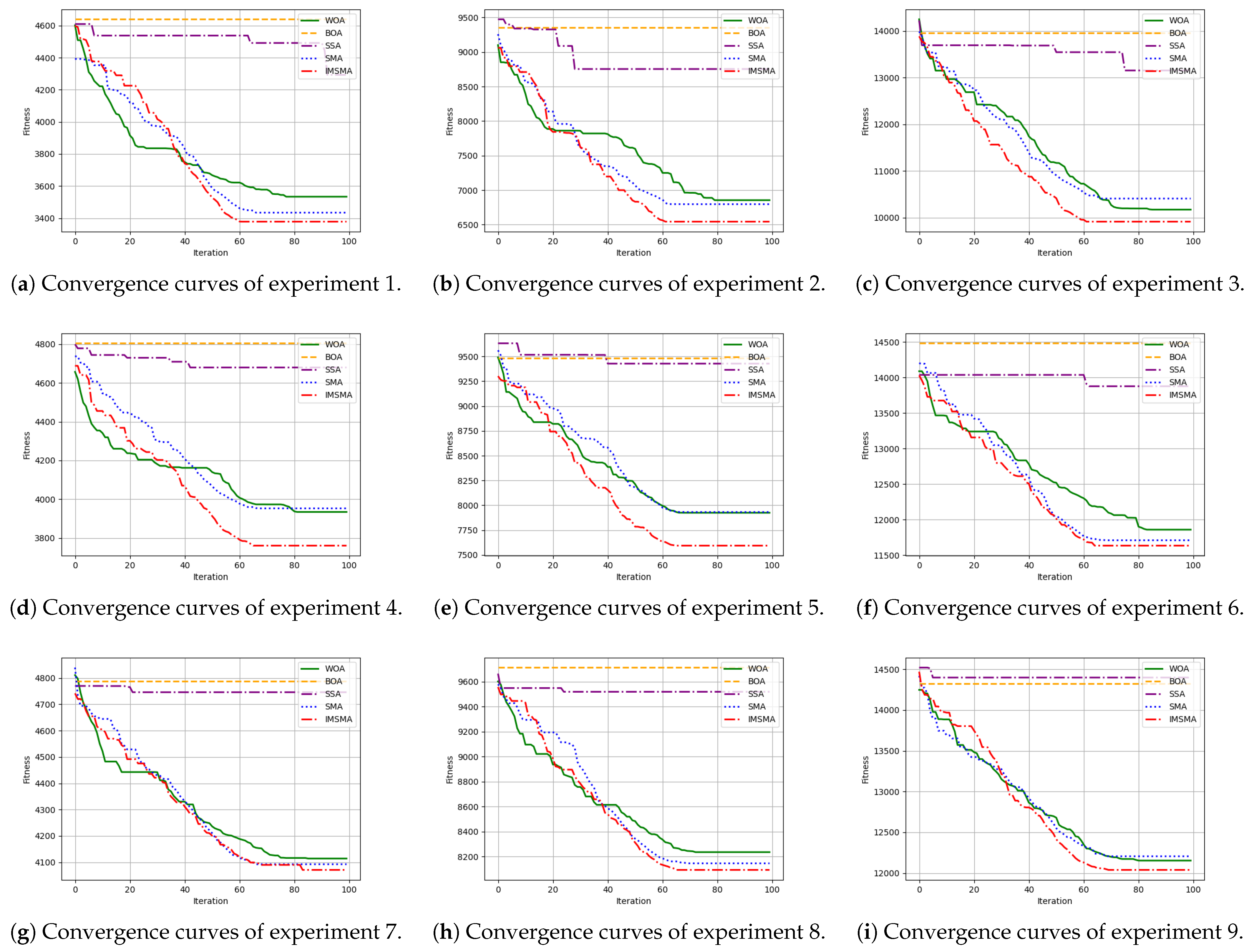
7. Numerical Experiment

We performed simulation experiments on the multiprocessor fair scheduling problem, with the same experimental environment as the performance testing of the improved slime mold algorithm. Assuming there were 1000 tasks and 10 processors with varying efficiencies, we randomly initialized a matrix $P_{ij}$ with dimensions 1000 rows by 10 columns. The elements of the matrix were set to values between 1 and 1000. The value at the ith row and jth column corresponded to the execution time of the ith task when executed on the jth processor. We used the IMSMA to solve the multiprocessor fair scheduling problem. The swarm size of the slime mold was fixed to 30, and the dimension was fixed to $n\times m$, which corresponded to the size of matrix $P_{ij}$.

Experiments were carried out on a range of problem sizes with a 100-iteration setting. The results for the objective values obtained by each algorithm are presented in

Table 4. Comparison of objective values obtained by different algorithms for various problem sizes.

Number of Experiments	n	m	IMSMA	SMA	WOA	BOA	SSA
Experiment 1	500	10	3378	3434	3534	4639	4293
Experiment 2	500	20	6544	6797	6854	9352	8753
Experiment 3	500	30	9915	10,409	10,173	13,966	13,155
Experiment 4	1000	10	3761	3953	3935	4804	4679
Experiment 5	1000	20	7593	7932	7925	9483	9428
Experiment 6	1000	30	11,634	11,709	11,858	14,483	13,878
Experiment 7	1500	10	4070	4092	4114	4788	4746
Experiment 8	1500	20	8092	8145	8235	9713	9519
Experiment 9	1500	30	12,038	12,205	12,152	14,321	14,398

.

The convergence curves of various algorithms for solving problems of different scales are shown in Figure 4.

Based on the data shown in Figure 4 and Table 4, it can be concluded that the IMSMA achieves the lowest objective function values and performs the best in solving the fair scheduling problem on multiple processors. The IMSMA effectively enhances the efficiency of solving the fair scheduling problem on multiple processors.

8. Conclusions

This paper investigated the fair scheduling problem on multiprocessors and proposed a new improved slime mold algorithm (IMSMA) built upon the original slime mold algorithm. The IMSMA introduces a population initialization strategy based on the Bernoulli mapping and reverse learning to enhance the population’s diversity of slime mold. It employs a Cauchy mutation strategy to facilitate escaping from local optima when the algorithm gets trapped. Furthermore, the boundary conditions of the slime mold algorithm were modified to nonlinear dynamic boundary conditions to improve the convergence efficiency and accuracy. Simulation experiments were conducted using two unimodal functions and two multimodal test functions to examine the algorithm’s effectiveness. The results demonstrated that the IMSMA exhibited a good convergence efficiency and the ability to escape local optima. Then, the paper modeled the fair scheduling problem on multiple processors, with the objective function set to minimize the average execution time on each processor. Finally, the IMSMA was utilized to solve the fair scheduling problem on multiple processors, and the outcomes were assessed against those of other algorithms. The comparison revealed that IMSMA achieved the best objective value and exhibited superior convergence performance compared to the other algorithms. The IMSMA can be applied not only to solve the fair scheduling problem on multiprocessors but also in various scenarios such as taxi dispatch systems and courier scheduling.

References

1. Agarwal, G.; Gupta, S.; Ahuja, R.; Rai, A.K. Multiprocessor task scheduling using multi-objective hybrid genetic Algorithm in Fog–cloud computing. Knowl.-Based Syst. 2023, 272, 110563. [Google Scholar]
2. Tang, Q.; Zhu, L.H.; Zhou, L.; Xiong, J.; Wei, J.B. Scheduling directed acyclic graphs with optimal duplication strategy on homogeneous multiprocessor systems. J. Parallel Distrib. Comput. 2020, 138, 115–127. [Google Scholar]
3. Fagin, R.; Williams, J.H. A fair carpool scheduling algorithm. IBM J. Res. Dev. 1983, 27, 133–139. [Google Scholar]
4. Alhussian, H.; Zakaria, N.; Hussin, F.A. An efficient real-time multiprocessor scheduling algorithm. J. Converg. Inf. Technol. 2014, 9, 136. [Google Scholar]
5. Li, T.; Baumberger, D.; Hahn, S. Efficient and scalable multiprocessor fair scheduling using distributed weighted round-robin. ACM Sigplan Not. 2009, 44, 65–74. [Google Scholar]
6. Nair, P.P.; Sarkar, A.; Biswas, S. Fault-tolerant real-time fair scheduling on multiprocessor systems with cold-standby. IEEE Trans. Dependable Secur. Comput. 2019, 18, 1718–1732. [Google Scholar]
7. Li, Z.; Bai, Y.; Liu, J.; Chen, J.; Chang, Z. Adaptive proportional fair scheduling with global-fairness. Wirel. Netw. 2019, 25, 5011–5025. [Google Scholar]
8. Wei, D.; Wang, Z.; Si, L.; Tan, C. Preaching-inspired swarm intelligence algorithm and its applications. Knowl.-Based Syst. 2021, 211, 106552. [Google Scholar]
9. Hou, J.; Liu, Z.; Wang, S.; Chen, Z.; Han, J.; Xie, W.; Fang, C.; Liu, J. Intelligent coordinated damping control in active distribution network based on PSO. Energy Rep. 2022, 8, 1302–1312. [Google Scholar]
10. Nasiri, J.; Khiyabani, F.M. A whale optimization algorithm (WOA) approach for clustering. Cogent Math. Stat. 2018, 5, 1483565. [Google Scholar]
11. Xue, J.; Shen, B. A novel swarm intelligence optimization approach: Sparrow search algorithm. Syst. Sci. Control Eng. 2020, 8, 22–34. [Google Scholar] [CrossRef]
12. Arora, S.; Singh, S. Butterfly optimization algorithm: A novel approach for global optimization. Soft Comput. 2019, 23, 715–734. [Google Scholar]
13. Dong, M.; Hu, J.; Yang, J.; Song, D.; Wan, J. Jiyu gaijin nianjun youhua shuanfa de guangfu duofeng MPPT kongzhi celue [Multi-peak MPPT Control Strategy for Photovoltaic Systems Based on Improved Slime Mould Optimization Algorithm]. Control Theory Appl. 2023, 40, 1440–1448. (In Chinese) [Google Scholar]
14. Premkumar, M.; Jangir, P.; Sowmya, R.; Alhelou, H.H.; Heidari, A.A.; Chen, H. MOSMA: Multi-objective slime mould algorithm based on elitist non-dominated sorting. IEEE Access 2020, 9, 3229–3248. [Google Scholar] [CrossRef]
15. Al-Qaness, M.A.; Ewees, A.A.; Fan, H.; Abualigah, L.; Abd Elaziz, M. Marine predators algorithm for forecasting confirmed cases of COVID-19 in Italy, USA, Iran and Korea. Int. J. Environ. Res. Public Health 2020, 17, 3520. [Google Scholar]
16. Li, S.; Chen, H.; Wang, M.; Heidari, A.A.; Mirjalili, S. Slime mould algorithm: A new method for stochastic optimization. Future Gener. Comput. Syst. 2020, 111, 300–323. [Google Scholar]
17. Gong, X.; Rong, Z.; Wang, J.; Zhang, K.; Yang, S. A hybrid algorithm based on state-adaptive slime mold model and fractional-order ant system for the travelling salesman problem. Complex Intell. Syst. 2023, 9, 3951–3970. [Google Scholar]
18. Chen, H.; Li, X.; Li, S.; Zhao, Y.; Dong, J. Improved slime mould algorithm hybridizing chaotic maps and differential evolution strategy for global optimization. IEEE Access 2022, 10, 66811–66830. [Google Scholar]
19. Abdel-Basset, M.; Chang, V.; Mohamed, R. HSMA_WOA: A hybrid novel Slime mould algorithm with whale optimization algorithm for tackling the image segmentation problem of chest X-ray images. Appl. Soft Comput. 2020, 95, 106642. [Google Scholar]
20. Gush, T.; Kim, C.H.; Admasie, S.; Kim, J.S.; Song, J.S. Optimal Smart Inverter Control for PV and BESS to Improve PV Hosting Capacity of Distribution Networks Using Slime Mould Algorithm. IEEE Access 2021, 9, 52164–52176. [Google Scholar] [CrossRef]
21. Vakilian, A.; Yalciner, M. Improved approximation algorithms for individually fair clustering. Proc. Mach. Learn. Res. 2022, 151, 8758–8779. [Google Scholar]
22. Zhong, J.H.; Peng, Z.P.; Li, Q.R.; He, J.G. Multi workflow fair scheduling scheme research based on reinforcement learning. Procedia Comput. Sci. 2019, 154, 117–123. [Google Scholar]
23. Xiao, Z.; Chen, L.; Wang, B.; Du, J.; Li, K. Novel fairness-aware co-scheduling for shared cache contention game on chip multiprocessors. Inf. Sci. 2020, 526, 68–85. [Google Scholar]
24. Salami, B.; Noori, H.; Naghibzadeh, M. Fairness-aware energy efficient scheduling on heterogeneous multi-core processors. IEEE Trans. Comput. 2020, 70, 72–82. [Google Scholar]
25. Mohtasham, A.; Filipe, R.; Barreto, J. FRAME: Fair resource allocation in multi-process environments. In Proceedings of the 2015 IEEE 21st International Conference on Parallel and Distributed Systems (ICPADS), Melbourne, Australia, 14–17 December 2015; pp. 601–608. [Google Scholar]
26. Jung, J.; Shin, J.; Hong, J.; Lee, J.; Kuo, T.W. A fair scheduling algorithm for multiprocessor systems using a task satisfaction index. In Proceedings of the International Conference on Research in Adaptive and Convergent Systems, Kraków, Poland, 20–23 September 2017; pp. 269–274. [Google Scholar]
27. Kanwal, S.; Inam, S.; Othman, M.T.B.; Waqar, A.; Ibrahim, M.; Nawaz, F.; Nawaz, Z.; Hamam, H. An Effective Color Image Encryption Based on Henon Map, Tent Chaotic Map, and Orthogonal Matrices. Sensors 2022, 22, 4359. [Google Scholar] [CrossRef]
28. Zhang, C.; Ding, S. A stochastic configuration network based on chaotic sparrow search algorithm. Knowl.-Based Syst. 2021, 220, 106924. [Google Scholar]
29. Yang, C.; Pan, P.; Ding, Q. Image encryption scheme based on mixed chaotic bernoulli measurement matrix block compressive sensing. Entropy 2022, 24, 273. [Google Scholar] [CrossRef]
30. He, J.; Guo, X.; Chen, H.; Chai, F.; Liu, S.; Zhang, H.; Zang, W.; Wang, S. Application of HSMAAOA Algorithm in Flood Control Optimal Operation of Reservoir Groups. Sustainability 2023, 15, 933. [Google Scholar]
31. Tizhoosh, H.R. Opposition-based learning: A new scheme for machine intelligence. In Proceedings of the International Conference on Computational Intelligence for Modelling, Control and Automation and International Conference on Intelligent Agents, Web Technologies and Internet Commerce (CIMCA-IAWTIC’06), Vienna, Austria, 28–30 November 2005; Volume 1, pp. 695–701. [Google Scholar]
32. Yu, H.; Song, J.; Chen, C.; Heidari, A.A.; Liu, J.; Chen, H.; Zaguia, A.; Mafarja, M. Image segmentation of Leaf Spot Diseases on Maize using multi-stage Cauchy-enabled grey wolf algorithm. Eng. Appl. Artif. Intell. 2022, 109, 104653. [Google Scholar]
33. Zhang, X.; Liu, Q.; Bai, X. Improved slime mould algorithm based on hybrid strategy optimization of Cauchy mutation and simulated annealing. PLoS ONE 2023, 18, e0280512. [Google Scholar]
Figure 1. Probability density functions for t-distribution, Gaussian distribution, and Cauchy distribution.
Algorithms 16 00473 g001
Figure 2. IMSMA Flowchart.
Algorithms 16 00473 g002
Figure 3. Curves of the test functions’ convergence.
Algorithms 16 00473 g003
Figure 4. Curves of test functions’ convergence.
Algorithms 16 00473 g004