A Greedy Pursuit Hierarchical Iteration Algorithm for Multi-Input Systems with Colored Noise and Unknown Time-Delays

Abstract

This paper focuses on the joint estimation of parameters and time delays for multi-input systems that contain unknown input delays and colored noise. A greedy pursuit hierarchical iteration algorithm is proposed, which can reduce the estimation cost. Firstly, an over-parameterized approach is employed to construct a sparse system model of multi-input systems even in the absence of prior knowledge of time delays. Secondly, the hierarchical principle is applied to replace the unknown true noise items with their estimation values, and a greedy pursuit search based on compressed sensing is employed to find key parameters using limited sampled data. The greedy pursuit search can effectively reduce the scale of the system model and improve the identification efficiency. Then, the parameters and time delays can be estimated simultaneously while considering the known orders and found locations of key parameters by utilizing iterative methods with limited sampled data. Finally, some simulations are provided to illustrate the effectiveness of the presented algorithm in this paper.

1. Introduction

System identification is a crucial process in modern control theory that involves determining the mathematical model of a system based on its input–output measurement data. The system identification is summarized and extended in references [1,2]. This modeling and estimation technique help engineers to estimate parameters that characterize system behavior, which can be used to design controllers for various applications. An efficient identification method is very important. The performance analysis of some algorithms for system identification is presented in [3], and some new identification methods based on multi-innovation theory are presented in [4]. Moreover, this technique has numerous practical applications across different fields such as aerospace engineering, robotics, and chemical processing plants. With the development of modern science and technology, the objects faced by system identification become increasingly complex. Those system models are defined as large-scale systems such as complex networks, neural networks, and artificial intelligence [5,6]. The parameter estimation of large-scale systems is an important research direction in system identification, where the reduced-order and decomposition are effective methods for identification of large-scale systems [7,8]. For instance, the neural network or artificial intelligence, which can be regarded as a class of typical large-scale systems, typically employ millions of interconnected neurons to simulate the brain. Similarly, the complex dynamic network control systems, characterized by a significant number of nodes and links, can also be considered as large-scale systems [9,10]. In conclusion, system identification plays an essential role in modern control theory by providing accurate mathematical models for complex systems. It allows us to predict outputs accurately while improving overall performance and efficiency across various systems. However, the difficulty of identification will increase with the increasingly dimensionality of the large-scale systems, which is a challenge that has to be faced in the future [11].

Large-scale systems usually contain a large number of variables. When these systems have unknown input time delays, the model used to describe them often includes redundant information. The identification problem for large-scale systems is typically divided into two stages: first, test measures are taken to estimate the orders and time delays; second, some identification algorithms are used to estimate the parameters. Therefore, traditional methods require prior knowledge such as system orders and time delays before estimating parameters. For example, the expectation maximization approach is used to estimate the parameters when the system orders and time-delay are known [12], the Bayesian method is used to estimate the system when the time-delay is known [13], and so does reference [14]. The least squares (LS) algorithms are widely used in large-scale system identification due to their fast parameter convergence rate and high estimation accuracy. The hierarchical LS iterative method is used to estimate the input nonlinear system [15,16], and the recursive LS estimation method is applied to identify the output nonlinear systems [17]. However, it should be noted that applying these methods directly can be difficult because there may be coupling items within large-scale systems. It is necessary to decouple the system before parameter estimation. A common approach is to decompose large-scale systems into some multi-variable subsystems; among these subsystems, multiple-input multiple-output (MIMO) systems are a typical class of multi-variable system. The MIMO systems can be decomposed into several single-input single-output (SISO) subsystems using decomposition techniques. Then, each of those subsystems can be identified one by one with enough sampled data [18], which comes with a huge computational cost. Another alternative approach for decomposing MIMO systems is to break them down into several multiple-input single-output (MISO) systems.

The identification problem of MISO systems has been extensively studied, and a large number of effective research results are given. Along with the emergence of compressed sensing (CS) in recent years, reference [19] gives the relevant basic of CS theory, reference [20] mainly introduces the principle and application of CS, and reference [21] presents the convergence of an interesting orthogonal matching pursuit (OMP) algorithm. The CS theory provides a new idea and some useful methods for system identification. For MISO systems that contain unknown input time delays, the parameter vector to be identified of the system that is over-parameterized has high dimension and sparse characteristics since the information vector contains unknown input delays. The CS is an effective idea to solve the parameter estimation for sparse systems. Many scholars have carried out research in related fields and achieved a series of results. Inspired by the greedy search idea of the CS, some parameter identification algorithms for output error models were designed by combining the auxiliary model and the hierarchical identification principle. For MISO output error systems with unknown time-delays, reference [22] combines a high dimensional and sparse estimation model with an auxiliary identification model to present the auxiliary model iterative algorithm, which has less computational cost compared with the auxiliary model least squires iterative, and reference [23] gives an auxiliary gradient pursuit iterative algorithm using the gradient search principle to further reduce the amount of computation. An iterative algorithm has been applied to achieve the estimation of time delays and parameters for multivariate systems output error systems by combining basis pursuit and auxiliary models in [24]. For MISO finite impulse response systems with input time delays, reference [25] combines the gradient search and matching pursuit method to give a gradient pursuit iterative algorithm and realize the parameters and time-delay estimation, and the gradient pursuit iterative algorithm can reduce the computational complexity compared with the traditional method. For nonlinear systems, a block-oriented nonlinear system was parameterized into a linear identification model including a sparse parameter vector, and the parameter estimation algorithm was presented by combining the matching pursuit idea based on CS, the auxiliary model, and key variable separation technology in [26]. For nonlinear systems containing colored noise in general, an OMP iterative method was presented to obtain the true parameters and time delays of an input Hammerstein nonlinear system in [27].

In this article, the kernel matrix is constructed to normalize the information matrix and satisfy the application conditions of compressed sensing, and a hierarchical iterative algorithm based on a greedy pursuit search idea is investigated to realize the parameters and time-delay estimation effectively at the same time [28]. The main innovations in this article are listed as follows.

• The multi-variable systems model is recast based on the framework of CS by using the hierarchical identification principle.
• The unknown true internal noise items of the recast sparse model in the presented algorithm are replaced by their estimation values according to the hierarchical principle.
• The presented algorithm constructs a kernel matrix to find the locations of key parameters and reduce the estimated dimension and computational cost by using greedy pursuit search, in which only limited sampled data are used.
• The parameters and time delays are estimated simultaneously by using the presented algorithm.

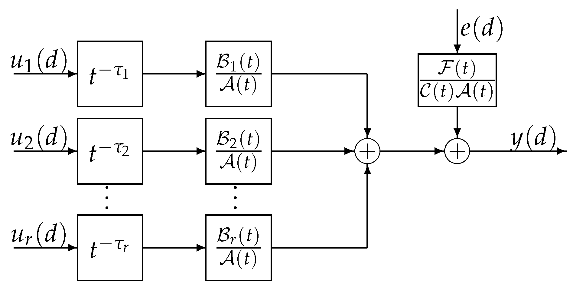
The remaining of this article is organized as follows. Section 2 introduces the multi-input system model with unknown input delays and colored noise. In Section 3, a greedy pursuit hierarchical iterative algorithm is given based on the over-parameterized sparse system model. In Section 4, some simulation experiments are given to show the effectiveness of the proposed method. Finally, Section 5 gives a summary of the content.

2. Systems Model

Consider the following systems shown in Figure 1.

The systems can be depicted as

$$\mathcal{A}\left(t\right)y\left(d\right)=\sum _{i=1}^r{t}^{-{\tau }_i}{\mathcal{B}}_i\left(t\right)u_i\left(d\right)+\frac{\mathcal{F}\left(t\right)}{\mathcal{C}\left(t\right)}e\left(d\right),$$

(1)

where $u_i\left(d\right)$ and $y\left(d\right)$ are the available input and output sampled data, and $e\left(d\right)$ is the noise satisfying $e\left(d\right)\sim N(0,{\sigma }^2)$, respectively. $\mathcal{A}\left(t\right),{\mathcal{B}}_i\left(t\right),\mathcal{C}\left(t\right),\mathcal{F}\left(t\right)$ are

$$\mathcal{A}\left(t\right):=1+\sum _{j=1}^{n_a}{a}_j{t}^{-j},{\mathcal{B}}_i\left(t\right):=\sum _{j=1}^{n_{bi}}{b}_{ij}{t}^{-j},\mathcal{C}\left(t\right):=1+\sum _{j=1}^{n_c}{c}_j{t}^{-j},\mathcal{F}\left(t\right):=1+\sum _{j=1}^{n_f}{f}_j{t}^{-j}.$$

where $n_a,n_{bi},n_c$, and $n_f$ are the system known orders and where the input time delay ${\tau }_i$ of each channel is unknown.

Introduce the internal noise item $w\left(d\right)$

$$\begin{array}{ccc}\hfill w\left(d\right)& :=& \frac{\mathcal{F}\left(t\right)}{\mathcal{C}\left(t\right)}e\left(d\right)=-\sum _{j=1}^{n_c}{c}_{j}w(d-j)+\sum _{j=1}^{n_f}{f}_{j}e(d-j)+e\left(d\right)\hfill \\ & =& {\mathit{\phi }}_n^{\mathrm{T}}\left(d\right){\mathit{\theta }}_n+e\left(d\right),\hfill \end{array}$$

(2)

where

$${\mathit{\phi }}_n\left(d\right):={[-w(d-1),-w(d-2),\cdots ,-w(d-n_c),e(d-1),e(d-2),\cdots ,e(d-n_f)]}^{\mathrm{T}}\in {\mathbb{R}}^{n_c+n_f},$$

(3)

$${\mathit{\theta }}_n:={[c_1,c_2,\cdots ,c_{n_c},f_1,f_2,\cdots ,f_{n_f}]}^{\mathrm{T}}\in {\mathbb{R}}^{n_c+n_f}.$$

(4)

The subscript n denotes noise.

Then, system model (1) can be rewritten as

$$y\left(d\right)=[1-A\left(t\right)]y\left(d\right)+\sum _{i=1}^r{t}^{-{\tau }_i}{\mathcal{B}}_i\left(t\right)u_i\left(d\right)+w\left(d\right).$$

(5)

Since the time delay of each input channel is unknown, define the data regression length l, which is large enough to satisfy $l⩾\max ({\tau }_i+n_{bi})$. Define the over-parameterized vector ${\mathit{\phi }}_s\left(t\right)$ and ${\mathit{\theta }}_s$ as

$${\mathit{\phi }}_s\left(d\right):={[{\mathit{\phi }}_a^{\mathrm{T}}\left(d\right),{\mathit{\phi }}_b^{\mathrm{T}}\left(d\right)]}^{\mathrm{T}}\in {\mathbb{R}}^{n_a+lr},$$

(6)

$${\mathit{\theta }}_s:={[{\mathit{\theta }}_a^{\mathrm{T}},{\mathit{\theta }}_b^{\mathrm{T}}]}^{\mathrm{T}}\in {\mathbb{R}}^{n_a+lr},$$

(7)

where

$$\begin{array}{c}{\mathit{\phi }}_a\left(d\right):={[-y(d-1),-y(d-2),\cdots ,-y(d-n_a)]}^{\mathrm{T}}\in {\mathbb{R}}^{n_a},\hfill \\ {\mathit{\phi }}_b\left(d\right):={[{\mathit{\phi }}_{b1}^{\mathrm{T}}\left(x\right),{\mathit{\phi }}_{b2}^{\mathrm{T}}\left(x\right),\cdots ,{\mathit{\phi }}_{br}^{\mathrm{T}}\left(x\right)]}^{\mathrm{T}}\in {\mathbb{R}}^{lr},\hfill \\ {\mathit{\phi }}_{bi}\left(d\right):={[u_i(d-1),\cdots ,u_i(d-{\tau }_i),u_i(d-{\tau }_i-1),\cdots ,u_i(d-{\tau }_i-n_{b_i}),\cdots ,u_i(d-l)]}^{\mathrm{T}}\in {\mathbb{R}}^l.\hfill \\ {\mathit{\theta }}_a:={[a_1,a_2,\cdots ,a_{n_a}]}^{\mathrm{T}}\in {\mathbb{R}}^{n_a},\hfill \\ {\mathit{\theta }}_b:={[{\mathit{\theta }}_{b1}^{\mathrm{T}},{\mathit{\theta }}_{b2}^{\mathrm{T}},\cdots ,{\mathit{\theta }}_{br}^{\mathrm{T}}]}^{\mathrm{T}}\in {\mathbb{R}}^{lr},{\mathit{\theta }}_{bi}:={[{\mathbf{0}}_{{\tau }_i},b_{i1},b_{i2},\cdots ,b_{i{n}_{bi}},{\mathbf{0}}_{l-{\tau }_i-n_{bi}}]}^{\mathrm{T}}\in {\mathbb{R}}^l,i=1,2,\cdots ,r.\hfill \end{array}$$

The subscript s denotes the system, and ${\mathbf{0}}_x$ denotes the zero block where the subscript means the number of zero elements.

Then, the following over-parameterized model can be indicated from Equation (5)

$$\begin{array}{c}\hfill y\left(d\right)={\mathit{\phi }}_s^{\mathrm{T}}\left(d\right){\mathit{\theta }}_s+w\left(d\right)={\mathit{\phi }}_s^{\mathrm{T}}\left(d\right){\mathit{\theta }}_s+{\mathit{\phi }}_n^{\mathrm{T}}\left(d\right){\mathit{\theta }}_n+e\left(d\right)\hfill \\ ={\mathit{\phi }}^{\mathrm{T}}\left(d\right)\mathit{\theta }+e\left(d\right),\hfill \end{array}$$

(8)

where

$$\begin{array}{c}\hfill \mathit{\phi }\left(d\right):={[{\mathit{\phi }}_s^{\mathrm{T}}\left(d\right),{\mathit{\phi }}_n^{\mathrm{T}}\left(d\right)]}^{\mathrm{T}}\in {\mathbb{R}}^N,N:=n_a+lr+n_c+n_f,\hfill \\ \mathit{\theta }:={[{\mathit{\theta }}_s^{\mathrm{T}},{\mathit{\theta }}_n^{\mathrm{T}}]}^{\mathrm{T}}\in {\mathbb{R}}^N.\hfill \end{array}$$

Consider the sampled data from $d=1$ to $d=L$ and define $\mathit{Y},\Phi ,\mathit{E}$ as

$$\begin{array}{c}\mathit{Y}:={[y\left(1\right),y\left(2\right),\cdots ,y\left(L\right)]}^{\mathrm{T}}\in {\mathbb{R}}^L,\hfill \\ \Phi :={[\mathit{\phi }\left(1\right),\mathit{\phi }\left(2\right),\cdots ,\mathit{\phi }\left(L\right)]}^{\mathrm{T}}\in {\mathbb{R}}^{L\times N},\hfill \\ \mathit{E}:={[e\left(1\right),e\left(2\right),\cdots ,e\left(L\right)]}^{\mathrm{T}}\in {\mathbb{R}}^L.\hfill \end{array}$$

The over-parameterized system model can be wrote as

$$\mathit{Y}=\Phi \mathit{\theta }+\mathit{E}.$$

(9)

Minimize the following cost function

$$J\left(\mathit{\theta }\right):=\sum _{j=1}^L{[y\left(j\right)-{\mathit{\phi }}^{\mathrm{T}}\left(j\right)\mathit{\theta }]}^2={\mathit{E}}^{\mathrm{T}}\mathit{E},$$

and the LS estimation value of the parameter vector will be obtained by using the LS principle

$$\widehat{\mathit{\theta }}={\left({\Phi }^{\mathrm{T}}\Phi \right)}^{-1}{\Phi }^{\mathrm{T}}\mathit{Y}.$$

(10)

Remark 1.

It is worth noting that Equation (10) cannot estimate the parameter directly as ${\mathit{\phi }}_n\left(d\right)$ contains unmeasurable internal noise items $w\left(d\right)$ and $e\left(d\right)$. In addition, the over-parameterized sparse system model has a large dimension N. Directly adopting the least squares method requires the sampled data to be much larger than the dimension N of the system model to achieve the satisfactory estimation accuracy. In some extreme cases, it will lead to matrix $\mathit{S}={\left[{\widehat{\Phi }}^{\mathrm{T}}\widehat{\Phi }\right]}^{-1}$ singularity when sufficient sampled data cannot be obtained. A large number of samples and high-dimensional matrix operations will increase the estimation cost.

In order to achieve high efficiency of parameters and time-delay estimation, this paper drives a greedy pursuit hierarchical iterative algorithm for system model (1) using limited sampled data according to the sparse property of the over-parameterized system model.

3. Greedy Pursuit Hierarchical Iterative Parameter Estimation Algorithm

The sparsity property of the over-parameterized system model makes it possible to identify the multi-input system with limited sampled data according to the compressed sensing idea. System model (9) can be rewrote as

$$\mathit{Y}=\sum _{j=1}^N{\mathit{\varphi }}_j{\theta }_j+\mathit{E},$$

(11)

where ${\mathit{\varphi }}_j$ and ${\theta }_j$ are the j-th column of $\Phi$ and the corresponding parameter in $\mathit{\theta }$. According to Equation (7), $\mathit{\theta }$ is sparse with a large number of zero elements and only contains a small number of non-zero key parameters. When the locations of the key parameters are found, the goal of reducing the dimensionality of the over-parameterized system model can be achieved. This provides the possibility of using limited sampling data to realize the parameters and time-delay estimation.

In order to meet the sparse recovery conditions, the information matrix $\Phi$ should be normalized. Define the normalized transformation matrix T as

$$\mathit{T}:={\left[\begin{array}{cccc}\Phi \left(1\right)& 0& \cdots & 0\\ 0& \Phi \left(2\right)& \cdots & 0\\ ⋮& 0& \ddots & ⋮\\ 0& 0& \cdots & \Phi \left(N\right)\end{array}\right]}^{-1}\in {\mathbb{R}}^{N\times N}$$

(12)

where $\Phi \left(j\right)=\sqrt{{\sum }_{i=1}^L{\Phi }_{ij}^2}$ denotes the modulus of the jth column of $\Phi$. Introducing T to Equation (9), the following can be obtained:

$$\mathit{Y}=\Psi \mathit{\vartheta }+\mathit{E},$$

(13)

where $\Psi =\Phi \mathit{T},\mathit{\vartheta }={\mathit{T}}^{-1}\mathit{\theta }$.

Let q be the inner iteration variable. Define the residual output as

$${\mathit{r}}_q:=\mathit{Y}-{\Psi }_{{\Lambda }_q}{\mathit{\vartheta }}_{{\Lambda }_q}.$$

(14)

where ${\Lambda }_q$ is an index set that is composed of the locations of the found key nonzero parameters, ${\Psi }_{{\Lambda }_q}$ is a sub-matrix of matrix $\Psi$, and ${\mathit{\vartheta }}_{{\Lambda }_q}$ is a non-zero parameter vector. Both ${\Psi }_{{\Lambda }_q}$ and ${\mathit{\vartheta }}_{{\Lambda }_q}$ are indexed by ${\Lambda }_q$. The sub-matrix ${\Psi }_{{\Lambda }_q}$ is composed of the indexed columns of the information matrix $\Psi$.

At the next internal iteration, define the following cost function and minimize it to find location of one key parameter.

$$J\left(j\right):=\parallel {\mathit{r}}_q-{\mathit{\psi }}_j{\vartheta }_j{\parallel }_2,$$

(15)

which lead to ${\vartheta }_j={\mathit{\psi }}_j{\mathit{r}}_q/{\parallel {\mathit{\psi }}_j\parallel }_2^2$. Plugged back ${\vartheta }_j$ into Equation (15), then we have

$$\begin{array}{c}\hfill J\left(j\right)=\underset{{\vartheta }_j}{\min }\parallel {\mathit{\psi }}_j{\vartheta }_j-{\mathit{r}}_q{\parallel }_2^2={\parallel \frac{{\mathit{\psi }}_j^{\mathrm{T}}{\mathit{r}}_q}{\parallel {\mathit{\psi }}_j{\parallel }_2^2}{\mathit{\psi }}_j-{\mathit{r}}_q\parallel }_2^2\hfill \\ = \parallel {\mathit{r}}_q{\parallel }_2^2-\frac{{\left({\mathit{\psi }}_j^{\mathrm{T}}{\mathit{r}}_q\right)}^2}{\parallel {\mathit{\psi }}_i{\parallel }_2^2}={\parallel {\mathit{r}}_q\parallel }_2^2-{\left({\mathit{\psi }}_j^{\mathrm{T}}{\mathit{r}}_q\right)}^2.\hfill \end{array}$$

(16)

where ${\mathit{\psi }}_j(j=1,2,\cdots ,N)$ is the column of the normalized matrix $\Psi$. From Equation (16), the column most relevant to the last iteration residual ${\mathit{r}}_q$ can be found at next iteration. That is, the minimum problem is equivalent to the largest inner product (in absolute value) between the columns of $\Psi$ and ${\mathit{r}}_q$. The location of found column can be indicated by the index

$${\lambda }_{q+1}=\arg \underset{j=1,2,\cdots ,N}{\max }\left|\langle {\mathit{r}}_q,{\mathit{\psi }}_j\rangle \right|.$$

(17)

Then, the index set and the index matrix can be updated according to ${\Lambda }_{q+1}:={\Lambda }_q\cup {\lambda }_{q+1}$.

Remark 2.

Because $w\left(d\right)$ and $e\left(d\right)$ in the matrix Φ are unknown noise items. The above steps from Equations (12)–(17) cannot be directly implemented since Φ contains some unknown items according to Equation (2).

Replace the true unmeasurable values $w\left(d\right)$ and $e\left(d\right)$ with their last iteration estimate by using the hierarchical principle [29]. Let k be the external iteration variable. ${\widehat{\mathit{\theta }}}_k,{\widehat{\mathit{\theta }}}_{k,s},{\widehat{\mathit{\theta }}}_{k,n}$ are iteration estimates of $\mathit{\theta },{\mathit{\theta }}_s,{\mathit{\theta }}_n$, respectively. By replacing d with $d-j$ in Equations (2) and (8), the following results can be obtained:

$$w(d-j)={\mathit{\phi }}_n^{\mathrm{T}}(d-j){\mathit{\theta }}_n+e(d-j),$$

(18)

$$y(d-j)={\mathit{\phi }}_s^{\mathrm{T}}(d-j){\mathit{\theta }}_s+w(d-j).$$

(19)

Then, the unknown noise items $w(d-j),e(d-j)$ can be replaced by their last estimate ${\widehat{w}}_{k-1}(d-j),{\widehat{e}}_{k-1}(d-j)$ based on Equation (3) and the hierarchical principle,

$$\begin{array}{c}\hfill {\widehat{\mathit{\phi }}}_{k,n}\left(d\right)=[-{\widehat{w}}_{k-1}(d-1),-{\widehat{w}}_{k-1}(d-2),\cdots ,-{\widehat{w}}_{k-1}(d-n_c),\hfill \\ {\widehat{e}}_{k-1}(d-1),{\widehat{e}}_{k-1}(d-2),\cdots ,{\widehat{e}}_{k-1}(d-n_f){]}^{\mathrm{T}}\in {\mathbb{R}}^{n_c+n_f}.\hfill \end{array}$$

(20)

Replace ${\mathit{\phi }}_n^{\mathrm{T}}(d-j),{\mathit{\theta }}_n,{\mathit{\theta }}_s$ with their iteration estimates ${\widehat{\mathit{\phi }}}_{k,n}^{\mathrm{T}}(d-j),{\widehat{\mathit{\theta }}}_{k,n},{\widehat{\mathit{\theta }}}_{k,s}$ in Equations (18) and (19); the estimation values of $w(d-j)$ and $e(d-j)$ at k-th iteration can be achieved by

$${\widehat{w}}_k(d-j)=y(d-j)-{\mathit{\phi }}_{k,s}^{\mathrm{T}}(d-j){\widehat{\mathit{\theta }}}_{k,s},$$

(21)

$${\widehat{e}}_k(d-j)={\widehat{w}}_k(d-j)-{\widehat{\mathit{\phi }}}_{k,n}^{\mathrm{T}}(d-j){\widehat{\mathit{\theta }}}_{k,n}.$$

(22)

According to Equation (20), the estimation of information matrix ${\widehat{\Phi }}_k$ can be denoted at the k-th external iteration, where ${\widehat{\mathit{\phi }}}_k\left(d\right)={[{\mathit{\phi }}_s^{\mathrm{T}}\left(d\right),{\widehat{\mathit{\phi }}}_{k,n}^{\mathrm{T}}\left(d\right)]}^{\mathrm{T}}$.

Use ${\widehat{\Phi }}_k$ to replace $\Phi$ in Equation (9). Construct the normalized transformation matrix $\widehat{\mathit{T}}$ using ${\widehat{\Phi }}_k$ based on Equation (12), and construct ${\widehat{\Psi }}_k$ according to ${\widehat{\Phi }}_k$ and $\widehat{\mathit{T}}$.

Then, Equations (14) and (15) can be expressed as

$${\mathit{r}}_{k,q}=\mathit{Y}-{\widehat{\Psi }}_{k,{\Lambda }_q}{\widehat{\mathit{\vartheta }}}_{k,{\Lambda }_q},$$

(23)

$${\lambda }_{k,q}=\arg \underset{j=1,2,\cdots ,N}{\max }\left|\langle {\mathit{r}}_{k,q-1},{\widehat{\mathit{\psi }}}_j\rangle \right|,$$

(24)

where the double subscripts $k,q$ denote that the key index at q inner iteration can be found using the kth external iteration updated data.

Applying the index set to update the normalization sub-matrix, we have

$${\widehat{\Psi }}_{k,{\Lambda }_q}={\widehat{\Psi }}_{k,{\Lambda }_{q-1}}\cup {\widehat{\mathit{\psi }}}_{k,{\lambda }_q},{\Lambda }_q={\Lambda }_{q-1}\cup {\lambda }_q.$$

(25)

Define a cost function as follows at the qth inner iteration to find the best parameter estimation value

$$J\left({\mathit{\vartheta }}_{k,{\Lambda }_q}\right)=\parallel {\mathit{r}}_{k,q}{\parallel }^2={\parallel \mathit{Y}-{\widehat{\Psi }}_{k,{\Lambda }_q}{\mathit{\vartheta }}_{k,{\Lambda }_q}\parallel }^2.$$

(26)

Minimize Equation (26), and the LS estimate can be obtained

$${\widehat{\mathit{\vartheta }}}_{k,{\Lambda }_q}={\left[{\widehat{\Psi }}_{k,{\Lambda }_q}^{\mathrm{T}}{\widehat{\Psi }}_{k,{\Lambda }_q}\right]}^{-1}{\widehat{\Psi }}_{k,{\Lambda }_q}^{\mathrm{T}}\mathit{Y}.$$

(27)

Note that ${\widehat{\mathit{\vartheta }}}_{k,{\Lambda }_q}\in {\mathbb{R}}^q$, using ${\Lambda }_{k,q}$ and the transformation matrix $\widehat{\mathit{T}}$, the over-parameterized sparse parameter vector can be obtained.

Then, the steps of the greedy pursuit hierarchical iterative (GPHI) algorithm are listed as follows.

• Define l and collect sampled data $\{u_i\left(d\right),y\left(d\right)$: $d=1,2,\cdots ,L\}$ to form Y.
• To initialize external iteration: let $k=1$, $\widehat{\mathit{\theta }}={\mathbf{1}}_N/p_0$, $p_0={10}^6$, ${\widehat{w}}_0\left(d\right),{\widehat{e}}_0\left(d\right)$ be a random number, and give allowable error $ϵ$ and $\epsilon$.
• Form ${\widehat{\mathit{\phi }}}_{k,n}\left(d\right)$ by Equation (20), and ${\widehat{\mathit{\phi }}}_k\left(d\right)$ by

  $${\widehat{\mathit{\phi }}}_k\left(d\right)={[{\mathit{\phi }}_s^{\mathrm{T}}\left(d\right),{\widehat{\mathit{\phi }}}_{k,n}^{\mathrm{T}}\left(d\right)]}^{\mathrm{T}}.$$

  (28)
  Using Equation (28), update ${\widehat{\Phi }}_k$, and using Equation (12) based on ${\widehat{\Phi }}_k$, construct $\widehat{\mathit{T}}$. Then, construct ${\widehat{\Psi }}_k$ by using ${\widehat{\Phi }}_k$ and $\widehat{\mathit{T}}$.
• Begin the internal iteration. Let $q=1$, ${\mathit{r}}_{k,0}=\mathit{Y}$, and ${\Lambda }_0=⌀$, ${\widehat{\Psi }}_{k,{\Lambda }_0}=⌀$.

  (a)

  Find ${\lambda }_q$ by Equation (24).

  (b)

  Update ${\Lambda }_q$ and ${\widehat{\Psi }}_{k,{\Lambda }_q}$ by Equation (25).

  (c)

  Compute the parameter estimate ${\widehat{\mathit{\vartheta }}}_{k,{\Lambda }_q}$ by Equation (27). Update residual $r_q$ by Equation (23).

  (d)

  If $\parallel {\widehat{\mathit{\vartheta }}}_{k,{\Lambda }_q}-{\widehat{\mathit{\vartheta }}}_{k,{ \Lambda }_{q-1}}\parallel ⩽ϵ$, obtain ${\widehat{\mathit{\vartheta }}}_{k,{\Lambda }_q}$; otherwise, increase q by 1 and go to step (a).

• Recover parameter estimate ${\widehat{\mathit{\theta }}}_k$ by

  $${\widehat{\mathit{\vartheta }}}_{k,{\Lambda }_q}\in {\mathbb{R}}^p\stackrel{{\Lambda }_q}{⟹}{\widehat{\mathit{\vartheta }}}_k\in {\mathbb{R}}^N,{\widehat{\mathit{\theta }}}_k=\widehat{\mathit{T}}{\widehat{\mathit{\vartheta }}}_k.$$

  (29)

  Update noise estimates ${\widehat{w}}_k(d-j),{\widehat{e}}_k(d-j)$ by Equations (21) and (22), and update the noise estimation vectors ${\widehat{\mathit{\phi }}}_{k,n}\left(d\right),{\widehat{\mathit{\phi }}}_k\left(d\right)$ using Equations (20) and (29), ${\widehat{\Phi }}_k$ and ${\widehat{\Psi }}_k$ by

  $${\widehat{\Phi }}_k={[{\widehat{\mathit{\phi }}}_k\left(1\right),{\widehat{\mathit{\phi }}}_k\left(2\right),\cdots ,{\widehat{\mathit{\phi }}}_k\left(L\right)]}^{\mathrm{T}},{\widehat{\Psi }}_k={\widehat{\Phi }}_k\widehat{\mathit{T}}.$$

  (30)
• If $\parallel {\widehat{\mathit{\theta }}}_k-{\widehat{\mathit{\theta }}}_{k-1}\parallel ⩽\epsilon$, complete the iteration stage and receive the final estimate $\widehat{\mathit{\theta }}$; otherwise, let $k=k+1$ and turn to step 4.

The recovered parameter vector $\widehat{\mathit{\theta }}$ has $r+1$ zero blocks. With prior knowledge l and orders $n_a,n_{bi}$, $n_c,n_f$, time-delay estimates will be received by

$$\begin{array}{c}{\widehat{\tau }}_1=n_1,\hfill \\ {\widehat{\tau }}_i=n_j-(l-{\widehat{\tau }}_{i-1}-n_{bj}),\hfill \end{array}$$

(31)

where $n_j(j=2,3,\cdots ,r)$ is the number of zero items in each zero block.

4. Simulation Experiments

Experiment 1. Consider a multi-input system as follows:

$$\begin{array}{ccc}\hfill \mathcal{A}\left(t\right)y\left(d\right)& =& \sum _{i=1}^5{t}^{{\tau }_i}{\mathcal{B}}_i\left(t\right)u_i\left(d\right)+\frac{\mathcal{F}\left(t\right)}{\mathcal{C}\left(t\right)}e\left(d\right),\hfill \\ \hfill \mathcal{A}\left(t\right)& =& 1+a_1{t}^{-1}+a_2{t}^{-2}=1-0.80t^{-1}+0.60t^{-2},\hfill \\ \hfill {\mathcal{B}}_1\left(t\right)& =& b_{11}{t}^{-1}+b_{12}{t}^{-2}=2.00t^{-1}-1.20t^{-2},\hfill \\ \hfill {\mathcal{B}}_2\left(t\right)& =& b_{21}{t}^{-1}+b_{22}{t}^{-2}=-1.80t^{-1}-0.90t^{-2},\hfill \\ \hfill {\mathcal{B}}_3\left(t\right)& =& b_{31}{t}^{-1}+b_{32}{t}^{-2}=1.00t^{-1}+0.50t^{-2},\hfill \\ \hfill \mathcal{C}\left(t\right)& =& 1+c_1{t}^{-1}=1+0.80t^{-1},\hfill \\ \hfill \mathcal{F}\left(t\right)& =& 1+f_1{t}^{-1}=1-0.40t^{-1}.\hfill \\ \hfill {\tau }_1& =& 6,{\tau }_2=15,{\tau }_3=20.\hfill \end{array}$$

Let $l=30$; the true value of the parameter vector to be estimated is

$$\mathit{\theta }={[-0.80,0.60,{\mathbf{0}}_6,2.00,-1.20,{\mathbf{0}}_{37},-1.80,-0.90,{\mathbf{0}}_{33},1.00,0.50,{\mathbf{0}}_8,0.80,-0.40]}^{\mathrm{T}}\in {\mathbb{R}}^N.$$

The $\left\{u_i\left(d\right)\right\}$ and $\left\{y\right(d\left)\right\}$ are measurable. The $e\left(d\right)\sim \mathcal{N}(0,{\sigma }^2)$ is noise, and the noise variances are taken to be ${\sigma }^2={0.50}^2$ and ${\sigma }^2={1.00}^2$, respectively. Take the sampled data length $L=1000$. The dimension of $\mathit{\theta }$ is $N:=n_a+lr+n_c+n_f=94$, where the sparsity is $K:=n_a+{\displaystyle \sum _{i=1}^5}{n}_{bi}+n_c+n_f=10$.

Use the first 200 sampled data to estimate this experiment by applying the GPHI algorithm, and the data from $d=200$ to $d=500$ are taken to verify the effectiveness of the obtained results. Define parameter estimation error as $\delta :=\parallel {\widehat{\mathit{\theta }}}_k-\mathit{\theta }\parallel /\mathit{\theta }\times 100\%$.

Noise variance is a commonly utilized metric for quantifying noise in measurement data, with higher values indicating reduced accuracy and reliability of the measurements. The impact of noise variance on parameter estimation accuracy cannot be overlooked. To evaluate the robustness of the GPHI algorithm against noise interference, the different noise variances ${\sigma }^2={0.50}^2$ and ${\sigma }^2={1.00}^2$ are applied.

The parameter estimates and estimation error $\delta$ versus iterative times k are shown in

Table 1. The estimated parameter values and estimation errors of Experiment 1 with $L=200$ (${\sigma }^2={0.50}^2$, ${\sigma }^2={1.00}^2$).

${\mathit{\sigma }}^2$	k	${\mathit{a}}_1$	${\mathit{a}}_2$	${\mathit{b}}_{11}$	${\mathit{b}}_{12}$	${\mathit{b}}_{21}$	${\mathit{b}}_{22}$	${\mathit{b}}_{31}$	${\mathit{b}}_{32}$	${\mathit{c}}_1$	${\mathit{f}}_1$	$\mathit{\delta }$%
${0.50}^2$	1	−0.7107	0.5090	1.9694	−1.0090	−1.8753	−1.0219	1.0790	0.5366	0.0000	0.0000	27.7831
	2	−0.8717	0.6218	1.9681	−1.3473	−1.8160	−0.7010	1.0268	0.3843	0.9248	0.0000	15.8395
	3	−0.7982	0.5895	1.9816	−1.1991	−1.7996	−0.8780	1.0396	0.4889	0.8053	0.0000	12.1355
	5	−0.8052	0.5905	1.9772	−1.2174	−1.7890	−0.8756	1.0339	0.4876	0.7704	−0.2763	3.9074
	8	−0.7905	0.5818	1.9615	−1.1770	−1.7950	−0.9001	1.0299	0.4972	0.7374	−0.4265	2.5213
${1.00}^2$	1	−0.5319	0.3512	1.9279	−0.6311	−1.9520	−1.3414	1.1347	0.6812	0.0000	0.0000	40.4417
	2	−1.1028	0.6513	1.9611	−1.7779	−1.8306	−0.1742	1.0516	0.0000	1.1758	0.0000	42.0247
	3	−0.7517	0.6354	1.9523	−1.1405	−1.8269	−0.9556	1.1100	0.5334	0.6873	0.0000	16.0285
	5	−0.8796	0.6296	1.9260	−1.3454	−1.8156	−0.7463	1.0452	0.4368	0.9477	0.0000	17.9049
	8	−0.8218	0.5847	1.9238	−1.2333	−1.7917	−0.8439	1.0565	0.4663	0.7521	−0.4519	4.0108
True values		−0.8000	0.6000	2.0000	−1.2000	−1.8000	−0.9000	1.0000	0.5000	0.8000	−0.4000

and Figure 2. From Figure 2, it can be seen that the estimation errors tend to decrease as the iterative times increase under different noise variances. The parameter estimates versus iterative times k are shown in Figure 3, Figure 4, Figure 5 and Figure 6.

From Figure 3, Figure 4, Figure 5 and Figure 6, it can be concluded that the estimated values gradually approach the true values with the increase in iterative times under different noise variances.

When noise variances are ${\sigma }^2={0.50}^2$ and ${\sigma }^2={1.00}^2$, the true outputs and estimated outputs versus iterative times k are given in Figure 7 and Figure 8, and a comparison of $\delta$ and the different sampled data length is shown in

Table 2. The estimation errors with different L and ${\sigma }^2$.

Sampled Data Length L	400	500	600	700	800	1000
Estimation error $\delta (\%)({\sigma }^2={0.50}^2)$	2.3931	2.591	2.0535	1.6165	1.9868	2.2789
Estimation error $\delta (\%)({\sigma }^2={1.00}^2)$	6.1781	5.9393	4.1059	4.3916	3.6913	4.5132

. When the system is disturbed by different noises, the estimated outputs can better match the true outputs and the bias of them is small—see Figure 7 and Figure 8.

With ${\sigma }^2={0.50}^2$ and $L=200$, the locations of the estimated key non-zero parameters are shown in

Table 3. The locations of the estimated key non-zero parameters of Experiment 1 with $L=200$ and ${\sigma }^2={0.50}^2$.

Parameter	${\widehat{\mathit{a}}}_1$	${\widehat{\mathit{a}}}_2$	${\widehat{\mathit{b}}}_{11}$	${\widehat{\mathit{b}}}_{12}$	${\widehat{\mathit{b}}}_{21}$	${\widehat{\mathit{b}}}_{22}$	${\widehat{\mathit{b}}}_{31}$	${\widehat{\mathit{b}}}_{32}$	${\widehat{\mathit{c}}}_1$	${\widehat{\mathit{f}}}_1$
Location	1	2	9	10	48	49	83	84	93	94

.

According to Table 3 and Equation (31), the time delays can be estimated

$$\begin{array}{c}\widehat{{\tau }_1}=n_1=6,\hfill \\ \widehat{{\tau }_2}=n_2-(l-\widehat{{\tau }_1}-n_{b2})=37-(30-6-2)=15,\hfill \\ \widehat{{\tau }_3}=n_3-(l-\widehat{{\tau }_2}-n_{b3})=33-(30-15-2)=20.\hfill \end{array}$$

(32)

Experiment 2. Consider the other multi-input system,

$$\begin{array}{ccc}\hfill A\left(t\right)y\left(d\right)& =& \sum _{i=1}^5{t}^{{\tau }_i}{B}_i\left(t\right)u_i\left(d\right)+\frac{F\left(t\right)}{C\left(t\right)}e\left(d\right),\hfill \\ \hfill A\left(t\right)& =& 1+a_1{t}^{-1}+a_2{t}^{-2}=1+0.60t^{-1}+0.4t^{-2},\hfill \\ \hfill B_1\left(t\right)& =& b_{11}{t}^{-1}+b_{12}{t}^{-2}=2.0t^{-1}-1.3t^{-2},\hfill \\ \hfill B_2\left(t\right)& =& b_{21}{t}^{-1}+b_{22}{t}^{-2}=1.5t^{-1}-0.9t^{-2},\hfill \\ \hfill B_3\left(t\right)& =& b_{31}{t}^{-1}+b_{32}{t}^{-2}=-1.0t^{-1}+0.5t{h}^{-2},\hfill \\ \hfill B_4\left(t\right)& =& b_{41}{t}^{-1}+b_{42}{t}^{-2}=-1.2t^{-1}+0.6t^{-2},\hfill \\ \hfill B_5\left(t\right)& =& b_{51}{t}^{-1}+b_{52}{t}^{-2}=1.0t^{-1}-0.8t^{-2},\hfill \\ \hfill C\left(t\right)& =& 1+c_1{t}^{-1}=1+0.7t^{-1},\hfill \\ \hfill F\left(t\right)& =& 1+f_1{t}^{-1}=1-0.4t^{-1}.\hfill \\ \hfill {\tau }_1& =& 9,{\tau }_2=23,{\tau }_3=15,{\tau }_4=30,{\tau }_5=17.\hfill \end{array}$$

Let the data regression length $l=50$. The true parameter vector to be identified is

$$\begin{array}{c}\hfill \mathit{\theta }=[0.60,0.40,{\mathbf{0}}_9,2.00,-1.30,{\mathbf{0}}_{62},1.50,-0.90,{\mathbf{0}}_{40},-1.00,0.50,{\mathbf{0}}_{63},-1.20,0.60,\hfill \\ {\mathbf{0}}_{35},1.00,-0.80,{\mathbf{0}}_{31}{,0.70,-0.40]}^{\mathrm{T}}\in {\mathbb{R}}^N.\hfill \end{array}$$

The dimension of sparse parameter vector is $N:=n_a+lr+n_c+n_f=254$, where the number of key non-zero parameters is $K:=n_a+{\displaystyle \sum _{i=1}^5}{n}_{bi}+n_c+n_f=14$. In this simulation, take the length of measurable input and output data $L=1000$. The data from $d=1$ to $d=250$ are used to realize the parameters and time-delay estimation. The remaining data from $d=250$ to $d=500$ are used to contrast the bias between the true outputs and estimated outputs. The other constraints are similar with those in Experiment 1.

To show the advantages of the GPHI algorithm, the errors $\delta$ of the LSI and GPHI algorithms versus the iteration times k are depicted in Figure 9, where sampled data length L is 250 and noise variance is ${\sigma }^2={0.50}^2$. From Figure 9, it can be found that the GPHI algorithm can achieve higher parameter estimation accuracy with limited sampled data.

When the noise variances are ${\sigma }^2={0.50}^2,{\sigma }^2={1.00}^2$, apply the GPHI algorithm. The errors $\delta$ versus k are shown in

Table 4. The estimated parameter values of parameter and errors of Experiment 2 with $L=250$ (${\sigma }^2={0.50}^2$, ${\sigma }^2={1.00}^2$).

${\mathit{\sigma }}^2$	k	${\mathit{a}}_1$	${\mathit{a}}_2$	${\mathit{b}}_{11}$	${\mathit{b}}_{12}$	${\mathit{b}}_{21}$	${\mathit{b}}_{22}$	${\mathit{b}}_{31}$	${\mathit{b}}_{32}$	${\mathit{b}}_{41}$	${\mathit{b}}_{42}$	${\mathit{b}}_{51}$	${\mathit{b}}_{52}$	${\mathit{c}}_1$	${\mathit{f}}_1$	$\mathit{\delta }$%
${0.50}^2$	1	0.7043	0.4193	1.9900	−1.1505	1.4756	−0.7222	−0.9542	0.3833	−1.2275	0.5137	0.9985	−0.6643	0.0000	0.0000	24.0379
	2	0.5958	0.3868	1.9909	−1.3471	1.4534	−0.8632	−0.9999	0.4732	−1.1926	0.5949	1.0018	−0.7892	0.8209	0.0000	11.8417
	3	0.5702	0.3731	1.9940	−1.4102	1.4709	−0.9009	−1.0007	0.5398	−1.1864	0.6208	0.9846	−0.8065	0.6720	−0.3408	3.8284
	5	0.5937	0.3974	1.9985	−1.3644	1.4680	−0.8740	−1.0119	0.5066	−1.1964	0.5860	0.9948	−0.7824	0.6427	−0.4213	2.6627
	8	0.5971	0.3944	1.9958	−1.3538	1.4675	−0.8662	−1.0131	0.5092	−1.1959	0.5802	0.9964	−0.7793	0.6478	−0.4059	2.4836
${1.00}^2$	1	1.1487	0.5378	1.9923	−0.3923	1.5176	0.0000	−0.9743	0.0000	−1.1962	0.0000	0.9823	0.0000	0.0000	0.0000	68.7931
	2	0.6610	0.3569	1.9489	−1.2599	1.4150	−0.7717	−1.0095	0.3747	−1.2543	0.5356	0.9832	−0.7020	0.7977	0.0000	15.6424
	3	0.5342	0.3111	1.9775	−1.5040	1.4303	−0.9078	−0.9906	0.5777	−1.1896	0.6985	1.0027	−0.8310	0.7349	−0.2909	7.8178
	5	0.5616	0.3767	2.0078	−1.4832	1.4422	−0.9073	−1.0159	0.5403	−1.2081	0.6244	0.9810	−0.8144	0.6377	−0.4610	5.8361
	8	0.6041	0.3931	1.9989	−1.3938	1.4410	−0.8344	−1.0317	0.5114	−1.2076	0.5711	0.9894	−0.7675	0.6391	−0.4123	4.0277
True values		0.6000	0.4000	2.0000	−1.3000	1.5000	−0.9000	−1.0000	0.5000	−1.2000	0.6000	1.0000	−0.8000	0.7000	−0.4000

and Figure 10, and the parameter estimates versus k are given in Figure 11, Figure 12, Figure 13 and Figure 14. Under different noise variances, the algorithm can achieve effective estimation accuracy of parameter estimation, and the parameter estimates approach the true values with the increase in the iterative times. This shows that the GPHI algorithm has certain robustness from Figure 10, Figure 11, Figure 12, Figure 13 and Figure 14.

Apply the data from $d=250$ to $d=500$ to verify the outputs with different noise variances. The true outputs, estimated outputs, and their bias are shown in Figure 15 and Figure 16, respectively. Figure 15 and Figure 16 show that the estimated output values can match the true values of the system well with different noise variances.

The errors $\delta$ versus different sampled data length L are shown in

Table 5. The parameter estimation errors with different L and ${\sigma }^2$.

Sampled Data Length L	300	400	500	600	700	800	1000
Estimation error $\delta (\%)({\sigma }^2={0.50}^2)$	2.3844	1.7831	1.9832	2.5122	2.4627	2.388	1.8807
Estimation error $\delta (\%)({\sigma }^2={1.00}^2)$	3.641	3.2164	4.055	4.7375	4.5741	4.1934	3.2887

to verify the validity of estimation accuracy under limited sampled data length. With ${\sigma }^2={0.50}^2$ and $L=250$, the key non-zero parameter location estimationsare given in

Table 6. The locations of the estimated key non-zero parameters of Experiment 2 with ${\sigma }^2={0.50}^2$ and $L=250$.

Parameter	${\widehat{\mathit{a}}}_1$	${\widehat{\mathit{a}}}_2$	${\widehat{\mathit{b}}}_{11}$	${\widehat{\mathit{b}}}_{12}$	${\widehat{\mathit{b}}}_{21}$	${\widehat{\mathit{b}}}_{22}$	${\widehat{\mathit{b}}}_{31}$	${\widehat{\mathit{b}}}_{32}$	${\widehat{\mathit{b}}}_{41}$	${\widehat{\mathit{b}}}_{42}$	${\widehat{\mathit{b}}}_{51}$	${\widehat{\mathit{b}}}_{52}$	${\widehat{\mathit{c}}}_1$	${\widehat{\mathit{f}}}_1$
Location	1	2	12	13	76	77	118	119	183	184	220	221	253	254

.

According to Table 6 and Equation (31), the time delays of Experiment 2 can be estimated

$$\begin{array}{ccc}\hfill \widehat{{\tau }_1}& =& n_1=9,\hfill \\ \hfill \widehat{{\tau }_2}& =& n_2-(l-\widehat{{\tau }_1}-n_{b2})=62-(50-9-2)=23,\hfill \\ \hfill \widehat{{\tau }_3}& =& n_3-(l-\widehat{{\tau }_2}-n_{b3})=40-(50-23-2)=15,\hfill \\ \hfill \widehat{{\tau }_4}& =& n_4-(l-\widehat{{\tau }_3}-n_{b4})=63-(50-15-2)=30,\hfill \\ \hfill \widehat{{\tau }_5}& =& n_5-(l-\widehat{{\tau }_4}-n_{b5})=35-(50-30-2)=17.\hfill \end{array}$$

(33)

Some results can be obtained from Figure 2, Figure 3, Figure 4, Figure 5, Figure 6, Figure 7, Figure 8, Figure 9, Figure 10, Figure 11, Figure 12, Figure 13, Figure 14, Figure 15 and Figure 16 and Table 1, Table 2, Table 3, Table 4, Table 5 and Table 6.

• With the increase in noise variance, the error of estimated parameter vector becomes bigger, but the estimation accuracy is still higher. This shows that the GPHI algorithm has certain robustness—see Figure 2 and Figure 9 and Table 1 and Table 4.
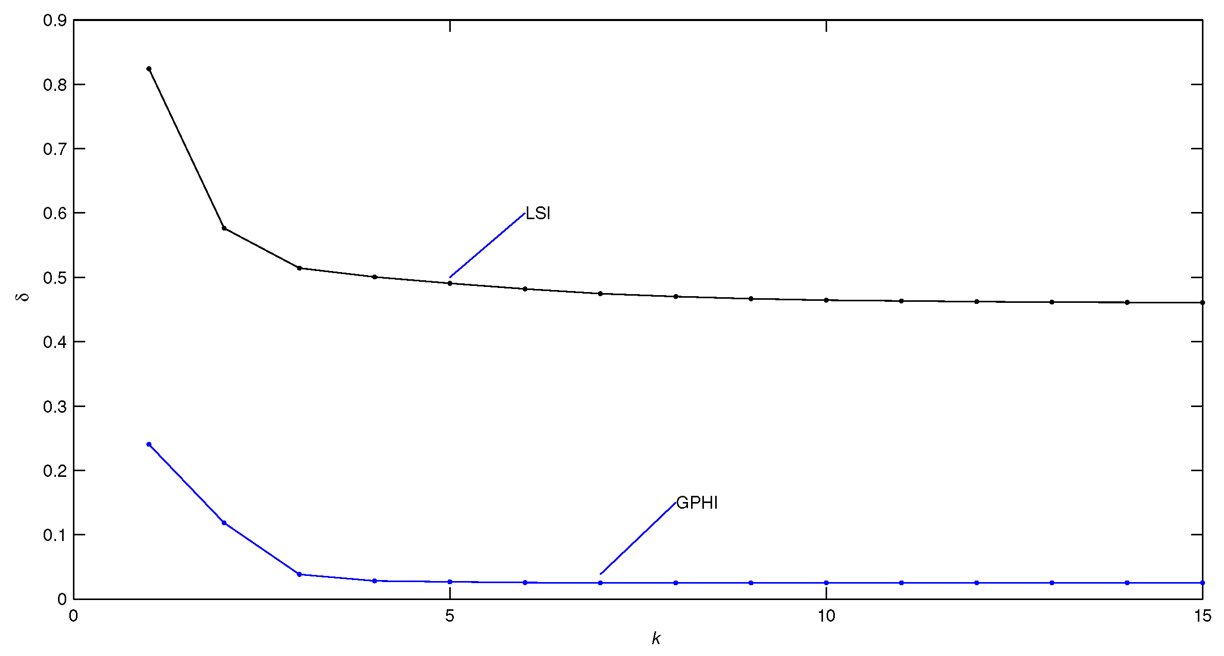
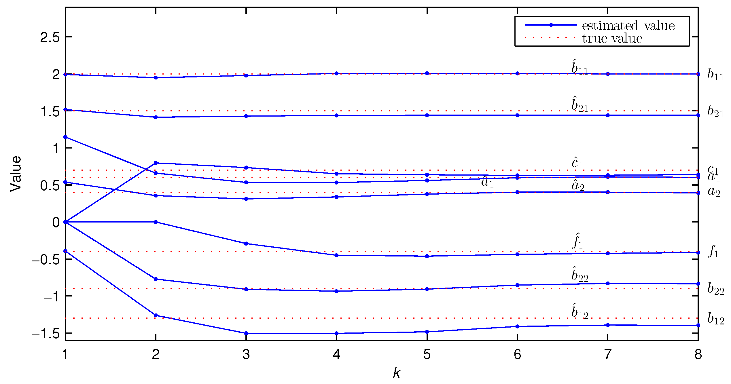
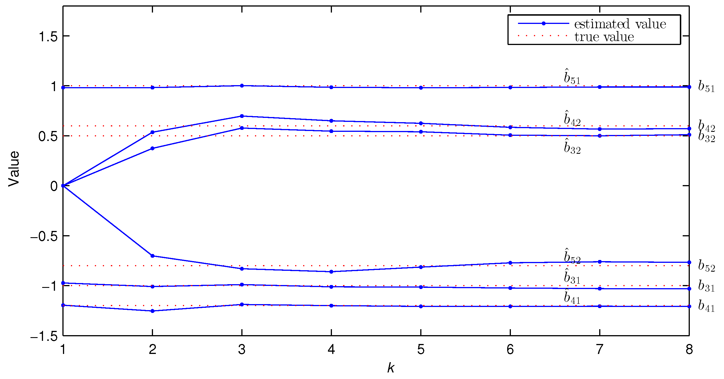
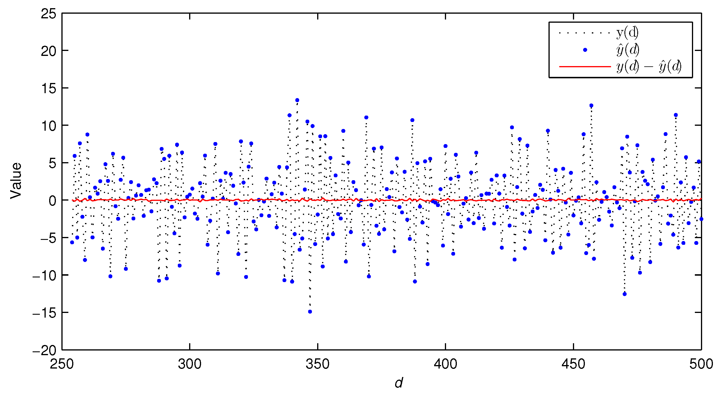
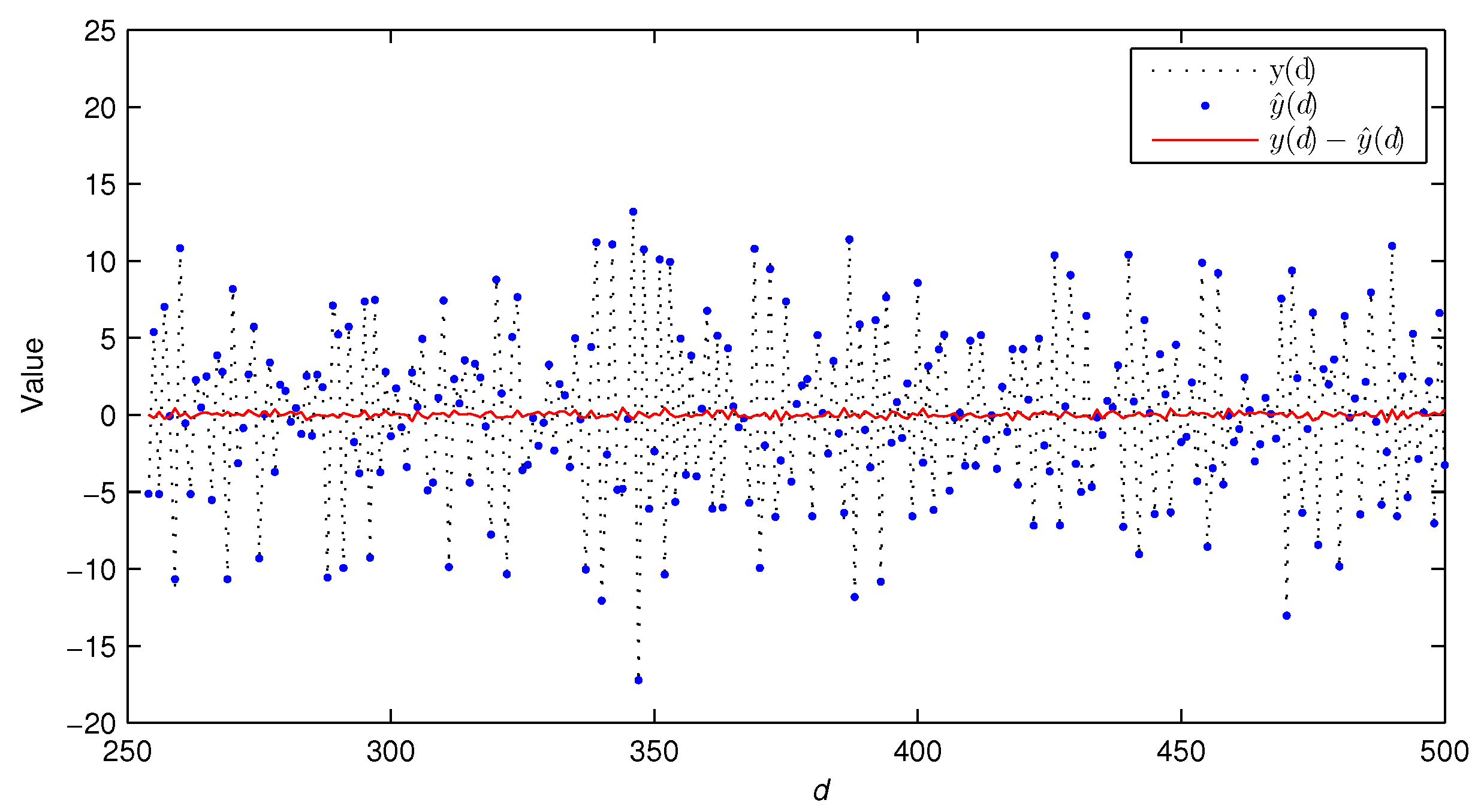
• Compared with the traditional LSI algorithm, the GPHI algorithm can use the limited sampled data to achieve higher parameter estimation accuracy—see Figure 9.
• With different noise variances, the parameter estimates converge near the true values as the iterative times increase, which shows that GPHI algorithm has certain robustness—see Figure 3, Figure 4, Figure 5, Figure 6, Figure 11, Figure 12, Figure 13 and Figure 14.
• The estimation accuracy of using limited sampled data is close to that of using large sampled data. This shows that the GPHI algorithm can realize parameter estimation using limited sampled data—see Table 2 and Table 5.
• The estimated outputs can match the true outputs well—see Figure 7, Figure 8, Figure 15 and Figure 16.
• The GPHI algorithm can accurately find the locations of key non-zero parameters, which shows that the GPHI algorithm can estimate the parameters and time delays simultaneously—see Table 3 and Table 6 and Equations (32) and (33).

5. Conclusions

This paper solves the problem of the joint estimation of parameters and time delays of a class of multi-input systems with colored noise by using limited sampled data. A hierarchical compressed sensing framework is established, and an efficient greedy pursuit hierarchical iterative algorithm is provided. Since the over-parameterized system model is sparse, the locations of key non-zero parameters can be found by using the greedy search method to reduce estimation cost, and the parameter estimates can be identified by using the iterative method. The time delays can be estimated based on prior knowledge combined with the structure of parameter estimates. Simulation examples demonstrate that the given algorithm can efficiently estimate parameters and time delays simultaneously.

References

1. Ljung, L. System Identification: Theory for The User, Information and System Science Series; Tsinghua University Press: Beijing, China, 2002. [Google Scholar]
2. Ding, F. System Identification—New Theory and Methods; Science Press: Beijing, China, 2013. [Google Scholar]
3. Ding, F. System Identification—Performance Analysis for Identification Methods; Science Press: Beijing, China, 2014. [Google Scholar]
4. Ding, F. System Identification—Multi-innovation Identification Theory and Methods; Science Press: Beijing, China, 2016. [Google Scholar]
5. Xu, J.; Tao, Q.; Li, Z.; Xi, X.; Suykens, J.A.; Wang, S. Efficient hinging hyperplanes neural network and its application in nonlinear system identification. Automatica 2020, 116, 108906. [Google Scholar] [CrossRef] [Green Version]
6. Zhang, C.M.; Lu, Y. Study on artificial intelligence: The state of the art and future prospects. J. Ind. Inf. Integr. 2021, 23, 00224. [Google Scholar] [CrossRef]
7. Chen, J.; Huang, B.; Gan, M.; Chen, P. A novel reduced-order algorithm for rational model based on Arnoldi process and Krylov subspace. Automatica 2021, 129, 109663. [Google Scholar] [CrossRef]
8. Li, Y.; Yu, K. Adaptive fuzzy decentralized sampled-data control for large-scale nonlinear systems. IEEE Trans. Fuzzy Syst. 2022, 30, 1809–1822. [Google Scholar] [CrossRef]
9. Skarding, J.; Gabrys, B.; Musial, K. Foundations and modeling of dynamic networks using dynamic graph neural networks: A survey. IEEE Access 2021, 9, 79143–79168. [Google Scholar] [CrossRef]
10. Liu, Y.A.; Tang, G.S.D.; Liu, Y.F.; Kong, Q.K.; Wang, J. Extended dissipative sliding mode control for nonlinear networked control systems via event-triggered mechanism with random uncertain measurement. Appl. Math. Comput. 2021, 396, 125901. [Google Scholar] [CrossRef]
11. Zhang, X.; Liu, Q.Y.; Ding, F.; Alsaedi, A.; Hayat, T. Recursive identification of bilinear time-delay systems through the redundant rule. J. Frankl. Inst. 2020, 357, 726–747. [Google Scholar] [CrossRef]
12. Gu, Y.; Liu, J.; Li, X.; Chou, Y.; Ji, Y. State space model identification of multirate processes with time-delay using the expectation maximization. J. Frankl. Inst. 2019, 356, 1623–1639. [Google Scholar] [CrossRef]
13. Fei, Q.L.; Ma, J.X.; Xiong, W.L.; Guo, F. Variational Bayesian identification for bilinear state space models with Markov-switching time delays. Int. J. Robust Nonlinear Control 2020, 30, 7478–7495. [Google Scholar] [CrossRef]
14. Ding, F.; Wang, X.H.; Mao, L.; Xu, L. Joint state and multi-innovation parameter estimation for time-delay linear systems and its convergence based on the Kalman filtering. Digit. Signal Process. 2017, 62, 211–223. [Google Scholar] [CrossRef]
15. Ding, F.; Ma, H.; Pan, J.; Yang, E.F. Hierarchical gradient and least squares-based iterative algorithms for input nonlinear output-error systems using the key term separation. J. Frankl. Inst. 2021, 358, 5113–5135. [Google Scholar] [CrossRef]
16. Ding, F.; Liu, X.M.; Hayat, T. Hierarchical least squares identification for feedback nonlinear equation-error systems. J. Frankl. Inst. 2020, 357, 2958–2977. [Google Scholar] [CrossRef]
17. Ding, F.; Wang, X.H.; Chen, Q.J.; Xiao, Y.S. Recursive least squares parameter estimation for a class of output nonlinear systems based on the model decomposition. Circ. Syst. Signal Process. 2016, 35, 3323–3338. [Google Scholar] [CrossRef]
18. Chen, T.; Ohlsson, H.; Ljung, L. On the estimation of transfer functions, regularizations and Gaussian processes—Revisited. Automatica 2012, 48, 1525–1535. [Google Scholar]
19. Donoho, D.L. Compressed sensing. IEEE Trans. Inf. Theory 2006, 52, 1289–1306. [Google Scholar]
20. Candès, E.J.; Wakin, M.B. An introduction to compressive sampling. IEEE Signal Process. Mag. 2008, 25, 21–30. [Google Scholar] [CrossRef]
21. Tropp, J.A. Greed is good: Algorithmic results for sparse approximation. IEEE Trans. Inf. Theory 2004, 50, 2231–2242. [Google Scholar] [CrossRef] [Green Version]
22. Liu, Y.J.; You, J.Y.; Ding, F. Iterative identification for multiple-input systems based on auxiliary model-orthogonal matching pursuit. Control Decis. 2019, 34, 787–792. [Google Scholar]
23. You, J.Y.; Liu, Y.J.; Chen, J.; Ding, F. Iterative identification for multiple-input systems with time-delays based on greedy pursuit and auxiliary model. J. Frankl. Inst. 2019, 356, 5819–5833. [Google Scholar]
24. You, J.Y.; Liu, Y.J. Iterative identification for multivariable systems with time-delays based on basis pursuit de-noising and auxiliary model. Algorithms 2018, 11, 180. [Google Scholar] [CrossRef]
25. Tao, T.Y.; Wang, B.; Wang, X.H. Parameter and time delay estimation algorithm based on gradient pursuit for multi-input C-ARMA systems. Control Decis. 2022, 37, 2085–2090. [Google Scholar]
26. Wang, D.Q.; Li, L.W.; Ji, Y.; Yan, Y. Model recovery for Hammerstein systems using the auxiliary model based orthogonal matching pursuit method. Appl. Math. Model. 2017, 54, 537–550. [Google Scholar] [CrossRef]
27. Mao, Y.W.; Ding, F.; Liu, Y.J. Parameter estimation algorithms for Hammerstein time-delay systems based on the orthogonal matching pursuit scheme. IET Signal Process. 2017, 11, 265–274. [Google Scholar] [CrossRef]
28. Troop, J.A. Just relax: Convex programming methods for identifying sparse signals in noise. IEEE Trans. Inf. Theory 2006, 52, 1030–1051. [Google Scholar] [CrossRef] [Green Version]
29. Ding, F. System Identification—Iterative Search Principle and Identification Methods; Science Press: Beijing, China, 2018. [Google Scholar]
Figure 1. The multi-input systems with input time delays and colored noise.
Algorithms 16 00374 g001
Figure 2. The estimation errors δ versus k of Experiment 1 with L = 200 ( σ 2 = 0.50 2 , σ 2 = 1.00 2 ).
Algorithms 16 00374 g002
Figure 3. The estimated parameter values a ^ 1 , a ^ 2 , c ^ 1 , f ^ 1 versus k of Experiment 1 with L = 200 and σ 2 = 0.50 2 .
Algorithms 16 00374 g003
Figure 4. The estimated parameter values b ^ 11 , b ^ 12 , b ^ 21 , b ^ 22 , b ^ 31 , b ^ 32 versus k of Experiment 1 with L = 200 and σ 2 = 0.50 2 .
Algorithms 16 00374 g004
Figure 5. The estimated parameter values a ^ 1 , a ^ 2 , c ^ 1 , f ^ 1 versus k of Experiment 1 with L = 200 and σ 2 = 1.00 2 .
Algorithms 16 00374 g005
Figure 6. The estimated parameter values b ^ 11 , b ^ 12 , b ^ 21 , b ^ 22 , b ^ 31 , b ^ 32 versus k of Experiment 1 with L = 200 and σ 2 = 1.00 2 .
Algorithms 16 00374 g006
Figure 7. The true outputs, estimated outputs, and their bias of Experiment 1 with σ 2 = 0.50 2 .
Algorithms 16 00374 g007
Figure 8. The true outputs, estimated outputs, and their bias of Experiment 1 with σ 2 = 1.00 2 .
Algorithms 16 00374 g008
Figure 9. The estimation errors of the LSI and GPHI algorithms versus k of Experiment 2 ( L = 250 , σ 2 = 0.50 2 ).
Algorithms 16 00374 g009
Figure 10. The estimation errors δ versus k of Experiment 2 with L = 250 and ( σ 2 = 0.50 2 , σ 2 = 1.00 2 ).
Algorithms 16 00374 g010
Figure 11. The estimated parameter values a ^ 1 , a ^ 2 , b ^ 11 , b ^ 12 , b ^ 21 , b ^ 22 , c ^ 1 , f ^ 1 versus k of Experiment 2 with L = 250 and σ 2 = 0.50 2 .
Algorithms 16 00374 g011
Figure 12. The estimated parameter values b ^ 31 , b ^ 32 , b ^ 41 , b ^ 42 , b ^ 51 , b ^ 52 versus k of Experiment 2 with L = 250 and σ 2 = 0.50 2 .
Algorithms 16 00374 g012
Figure 13. The estimated parameter values a ^ 1 , a ^ 2 , b ^ 11 , b ^ 12 , b ^ 21 , b ^ 22 , c ^ 1 , f ^ 1 versus k of Experiment 2 with L = 250 and σ 2 = 1.00 2 .
Algorithms 16 00374 g013
Figure 14. The estimated parameter values b ^ 31 , b ^ 32 , b ^ 41 , b ^ 42 , b ^ 51 , b ^ 52 versus k of Experiment 2 with L = 250 and σ 2 = 1.00 2 .
Algorithms 16 00374 g014
Figure 15. The true outputs, estimated outputs, and their bias of Experiment 2 with σ 2 = 0.50 2 .
Algorithms 16 00374 g015
Figure 16. The true outputs, estimated outputs, and their bias of Experiment 2 with σ 2 = 1.00 2 .
Algorithms 16 00374 g016