Ascertaining the Ideality of Photometric Stereo Datasets under Unknown Lighting

Abstract

The standard photometric stereo model makes several assumptions that are rarely verified in experimental datasets. In particular, the observed object should behave as a Lambertian reflector, and the light sources should be positioned at an infinite distance from it, along a known direction. Even when Lambert’s law is approximately fulfilled, an accurate assessment of the relative position between the light source and the target is often unavailable in real situations. The Hayakawa procedure is a computational method for estimating such information directly from data images. It occasionally breaks down when some of the available images excessively deviate from ideality. This is generally due to observing a non-Lambertian surface, or illuminating it from a close distance, or both. Indeed, in narrow shooting scenarios, typical, e.g., of archaeological excavation sites, it is impossible to position a flashlight at a sufficient distance from the observed surface. It is then necessary to understand if a given dataset is reliable and which images should be selected to better reconstruct the target. In this paper, we propose some algorithms to perform this task and explore their effectiveness.

1. Introduction

Photometric stereo (which we will denote by PS) is a classic computer vision approach for reconstructing the shape of a three-dimensional object [1,2]. It is considered a shape from shading (SfS) technique, as it takes as input images that embed the shape and color information of the observed object. However, while the original SfS problem only considers a single two-dimensional image of the object [3,4] and it is known to be ill-posed, PS stands on the use of a set of images acquired from a fixed point of view under varying lighting conditions.

If the lighting positions are known, Kozera [5] proved that, under suitable assumptions, the PS problem is well-posed when at least two pictures are available. Kozera’s approach consists of modeling the problem by a system of first-order Hamilton-Jacobi partial differential equations (PDEs), for which various numerical methods have been proposed (see, e.g., [6]). The solution process that we will consider is slightly different and operates in two steps. First, the normal vectors at each discretization point of a rectangular domain, namely, the digital picture, are determined by solving an algebraic matrix equation. Then, after numerically differentiating the normal vector field, the solution of a Poisson PDE leads to the approximation of the object surface. This approach has been used in [7] to reconstruct rock art carvings found in Domus de Janas (fairy houses), a specific typology of Neolithic tombs found in Sardinia, Italy [8]. While this computational scheme requires at least three images with different lighting conditions, the availability of a larger dataset leads to a least-squares solution method, which allows for a more efficient treatment of measurement errors.

Though in the research community, the position of the light sources is generally assumed to be known [9,10,11], real-world applications of PS often deal with datasets acquired under unknown light conditions [12,13]. In [14], Hayakawa has shown that the lighting directions can be identified directly from the data when at least six images with different illumination are available (see [14] and Section 2 for a proof), yielding the possibility to apply PS to field measurement scenarios, as in the case of archaeological excavations [15].

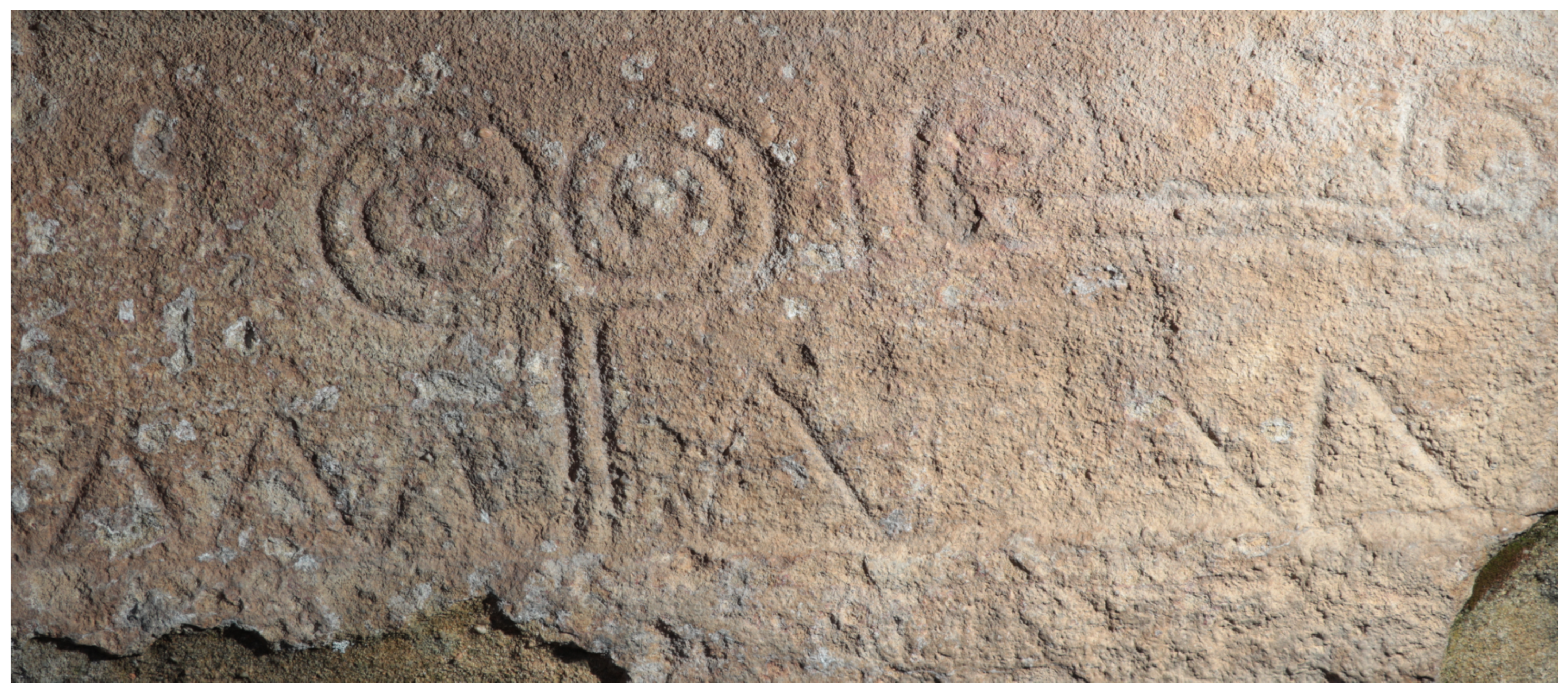
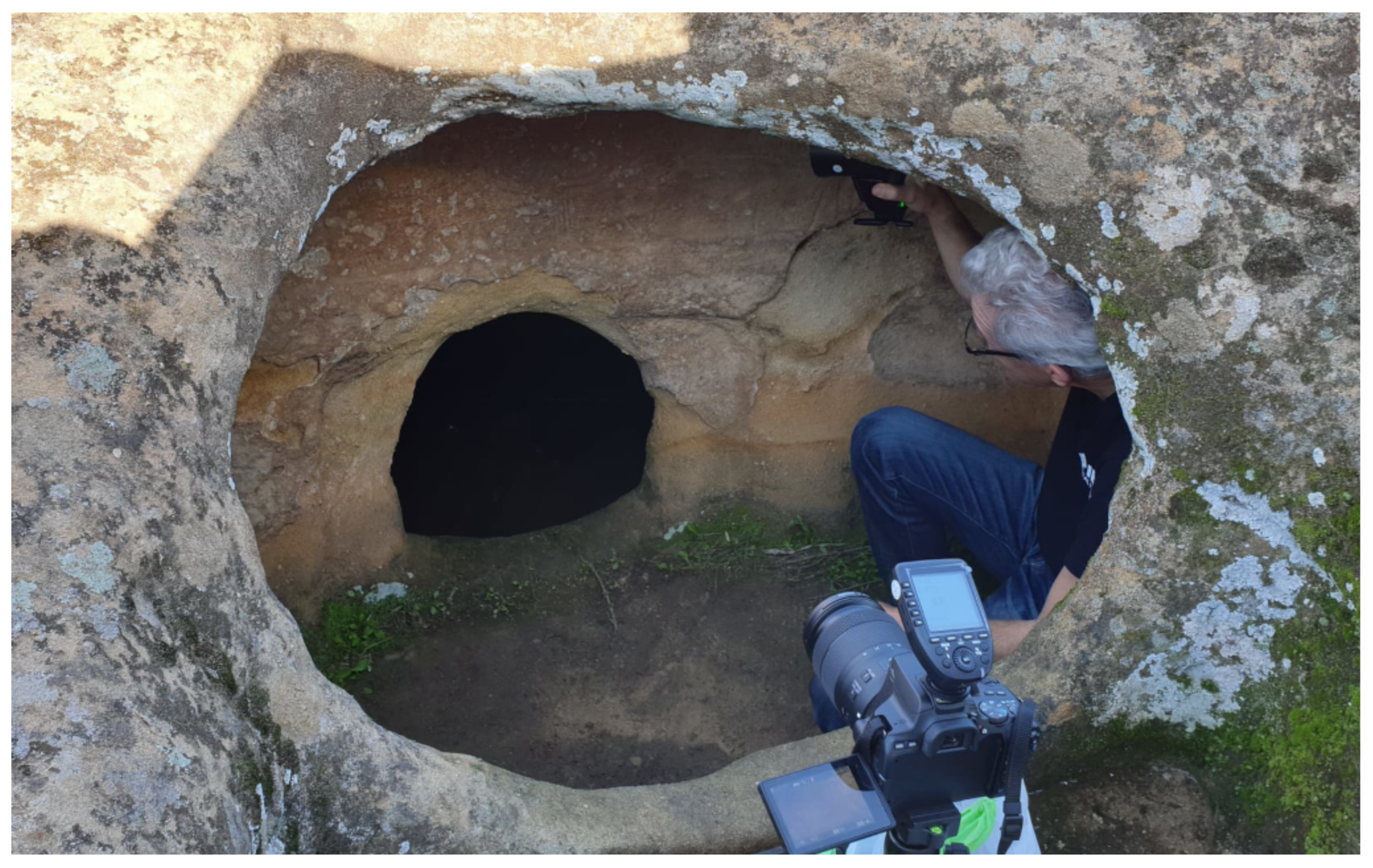
For example, the bas-relief displayed in Figure 1 is found in the Domus de Janas of Corongiu, in Pimentel (South Sardinia, Italy), dated 4th millennium BC. Figure 2 shows the small lobby where the engraving is located. While the camera can be placed sufficiently far from the rock surface, it is impossible to illuminate it with a flashlight at a distance suitable for proper lighting. Moreover, measuring with precision the position of the light source relative to the engraving is very difficult. This situation is common in many archaeological sites.

PS application implies that certain assumptions are met in the acquisition process. In general, a perspective camera projection model may be used, with parameters estimated by camera calibration methods (see [16] for an introduction to the use of perspective and [10,17] for applications). In this work, we consider an orthographic camera model, which simplifies the presentation and is suitable for situations where the camera can be positioned at a relatively far distance from the observed object. The mathematical formulation of PS assumes that the object surface is Lambertian, meaning that Lambert’s cosine law can be employed to describe the object reflectance. This condition implies that the surface is matte and free from specular reflections, which is seldom verified in practice (see [18,19,20], where the Oren–Nayar model has been used to preprocess a dataset originated by a non-Lambertian object).

Many studies have been devoted to improving the application of PS to non-Lambertian conditions. In [21], the authors formulate the problem as a low-rank matrix factorization subject to sparse errors, due to the presence of shadows and specular reflections in data images. A statistical approach based on a hierarchical Bayesian approximation was used in [22] to simultaneously estimate the surface normal vectors and the experimental errors, by solving a constrained sparse regression problem. Learning-based methods were also employed to solve PS (see, e.g., [23,24]). To manage near-light problems, models based on neural networks were presented in [25,26], where they were stated under non- Lambertian conditions.

Our approach is slightly different from the ones above. Here, we assume that the light source location is unknown, and point our attention to the lack of ideality in a dataset due to either the necessity of illuminating the observed surface with close lights, or to the fact that the surface is only approximately Lambertian. Indeed, in archaeological applications, which motivated this work, the assumption that requires the light sources to be located at a large distance (theoretically, at infinite distance) from the observed surface is an unacceptable constraint, as carvings and bas-reliefs are often located in narrow caves or excavations. Furthermore, the carvings are engraved in rock, which may not be an ideal Lambertian surface. To explore these aspects of the model, we assume that orthographic projection conditions are met and the position of light sources is unknown. Then, we determine the light position by the Hayakawa procedure and investigate the reason for its breakdown in the presence of nonideal data, i.e., images that excessively deviate from the above assumption. This also leads us to introduce a new nonlinear approach for identifying the light position, alternative to Hayakawa’s one. Finally, we study the problem of ascertaining the ideality of a dataset. This is accomplished by defining some measures of ideality, which can assist a researcher in selecting the best subset of images from a redundant dataset. To demonstrate the performance of the new approaches, we apply them to both a synthetic dataset, where the position of the lights can be decided at will, and to an experimental one, which is not guaranteed to represent a Lambertian reflector.

The plan of the paper is the following. Section 2 contains a review of the numerical procedures to solve the PS problem under both known and unknown lighting. In Section 3, we describe a new nonlinear approach to determine the light position directly from the available data. The ideality of a dataset is discussed in Section 4, where two indicators are introduced for detecting the presence of unideal images, and an algorithm is presented to extract a subset of pictures that better suit the assumptions of the PS model. The numerical experiments that investigate the performance of the algorithm are outlined in Section 5 and discussed in Section 6.

2. A Review of the Hayakawa Procedure for Determining the Light Position

In this section, we briefly review the mathematical model implementing Lambert’s law that is usually adopted in photometric stereo under the assumption of orthographic projection and light source at an infinite distance from the target (see [15] for more details). We also outline the Hayakawa procedure [14] for estimating the lighting directions from the data.

Let us associate an orthonormal reference system to ${\mathbb{R}}^3$ and assume the observed object is located at its origin. The optical axis of the camera coincides with the z-axis, and the point of view is at infinite distance, to ensure orthographic projection. The camera has a resolution of $(r+2)\times (s+2)$ pixels, and is associated with the rectangular domain $\mathrm{\Omega }=\left[-A/2,A/2\right]\times \left[-B/2,B/2\right]$, where A is the horizontal size of the rectangle and $B=(s+1)h$, with $h=A/(r+1)$. The domain discretization consists of a grid of points with coordinates $(x_i,y_j)$, for $i=0,\dots ,r+1$ and $j=0,\dots ,s+1$, given by

$$x_i=-\frac{A}{2}+ih,y_j=-\frac{B}{2}+jh.$$

(1)

The surface of the object is represented by a bivariate explicit function $z=u(x,y)$, $(x,y)\in \mathrm{\Omega }$, whose partial derivatives are denoted by $u_x$ and $u_y$. Then, the gradient of u and the (normalized) normal vector to each point of the surface are defined as

$$\nabla u(x,y)=\left[\begin{array}{c}{u}_x\\ u_y\end{array}\right]\mathrm{and}\mathbf{n}(x,y)=\frac{{[-u_x,-u_y,1]}^T}{\sqrt{1+{\parallel \nabla u\parallel }^2}},$$

respectively, where $\parallel ·\parallel$ denotes the 2-norm. All functions are discretized on the grid, and their values are stacked in a vector in lexicographic order, that is, according to the rule $k=(i-1)s+j$, where $k=1,\dots ,p$, and p denotes the number of pixels in the image. We will write indifferently $u(x_i,y_j)$, $u_{i,j}$, or $u_k$, and similarly for $u_x(x_i,y_j)$, $u_y(x_i,y_j)$, and $\mathbf{n}(x_i,y_j)$.

The images in the dataset are stacked in the vectors ${\mathbf{m}}_t\in {\mathbb{R}}^p$, $t=1,\dots ,q$. In each of the pictures, the target is illuminated by a light source located in a different direction. We denote the vector that points from the object to the light source by ${\mathcal{l}}_t={[{\mathcal{l}}_{1t},{\mathcal{l}}_{2t},{\mathcal{l}}_{3t}]}^T$, with $t=1,\dots ,q$. Its 2-norm is proportional to the light intensity. To simplify notation, in the following, we assume the light vectors to be normalized, that is, $\parallel {\mathcal{l}}_t\parallel =1$.

Assuming that the observed surface is a Lambertian reflector, we state Lambert’s cosine law in the form

$$\rho (x,y)\langle \mathbf{n}(x,y),{\mathcal{l}}_t\rangle =I_t(x,y),t=1,\dots ,q,$$

(2)

where $\langle ·,·\rangle$ is the standard inner product in ${\mathbb{R}}^3$, and the albedo $\rho (x,y)$ accounts for the partial light absorption of the surface, due to its color or material. After discretization, Formula (2) reads

$${\rho }_k{\mathbf{n}}_k^T{\mathcal{l}}_t=m_{kt},k=1,\dots ,p,t=1,\dots ,q,$$

(3)

where $m_{kt}$ represents the kth component of the image vector ${\mathbf{m}}_t$, that is, the radiation $I_t(x_i,y_j)$ reflected by a neighborhood of the kth pixel in the image number t.

Equations (3) can be represented in the form of the matrix equation

$$D{N}^{T}L=M,$$

(4)

after assembling data and unknowns in the matrices

$$\begin{array}{cccc}\hfill D& =diag({\rho }_1,\dots ,{\rho }_p)\in {\mathbb{R}}^{p\times p},\hfill & \hfill L& =\left[{\mathcal{l}}_1,\dots ,{\mathcal{l}}_q\right]\in {\mathbb{R}}^{3\times q},\hfill \\ \hfill N& =\left[{\mathbf{n}}_1,\dots ,{\mathbf{n}}_p\right]\in {\mathbb{R}}^{3\times p},\hfill & \hfill M& =\left[{\mathbf{m}}_1,\dots ,{\mathbf{m}}_q\right]\in {\mathbb{R}}^{p\times q}.\hfill \end{array}$$

If the matrix L, whose columns are the vectors aiming at the lights, is known, one usually sets $\tilde{N}=ND$ in (4), and computes ${\tilde{N}}^T=M{L}^{†}$, where $L^{†}$ denotes the Moore–Penrose pseudoinverse of L [27]. This produces a unique solution if $q\ge 3$ and the matrix L is full-rank. Once $\tilde{N}$ is available, by normalizing its columns, one easily obtains N and D from which, by integrating the normal vectors (see [28]), the approximation of the surface representation $u(x,y)$ at the discretization grid can be computed.

When the light positions are not known, the Hayakawa procedure [14] can be used to estimate this information from the data, but this requires the availability of at least six images with different lighting conditions. Here, we briefly summarize this technique (see [15] for more details).

To obtain an initial Rank-3 factorization of the data matrix M, we start computing the singular value decomposition (SVD) [29]

$$M=U\Sigma V^T,$$

(5)

where $\Sigma =diag({\sigma }_1,\dots ,{\sigma }_q)$ contains the singular values ${\sigma }_1\ge \dots \ge {\sigma }_q\ge 0$, and $U\in {\mathbb{R}}^{p\times q}$, $V\in {\mathbb{R}}^{q\times q}$ are matrices with orthonormal columns ${\mathbf{u}}_i$, ${\mathbf{v}}_i$. Theoretically, only the first three singular values should be positive, that is, ${\sigma }_4=\dots ={\sigma }_q=0$. Anyway, because of experimental errors propagation and lack of ideality in the data, one usually finds ${\sigma }_i>0$, $i=4,\dots ,q$.

It is known that the best Rank-k approximation of a matrix with respect to both the 2-norm and the Frobenius norm is produced by truncating the SVD to k terms [27]. So, we define $W={[{\sigma }_1{\mathbf{u}}_1,{\sigma }_2{\mathbf{u}}_2,{\sigma }_3{\mathbf{u}}_3]}^T$ and $Z={[{\mathbf{v}}_1,{\mathbf{v}}_2,{\mathbf{v}}_3]}^T$, to obtain the Rank-3 approximation $W^{T}Z$ of M.

Following the proof of Theorem 1 from [15], we consider the factorization $W^{T}Z=M$ as a tentative approximation of ${\tilde{N}}^{T}L=M$. Assuming $\parallel {\mathcal{l}}_t\parallel =1$, we seek a matrix B such that

$$\parallel B{\mathbf{z}}_t\parallel =1,t=1,\dots ,q,$$

(6)

where ${\mathbf{z}}_t\in {\mathbb{R}}^3$, $t=1,\dots ,q$, denote the columns of Z.

The Hayakawa procedure consists of writing Problem (6) in the form

$$diag\left(Z^{T}GZ\right)=\mathbf{1},$$

(7)

where $\mathbf{1}={[1,\dots ,1]}^T\in {\mathbb{R}}^q$ and $G=B^{T}B$ is a symmetric positive definite $3\times 3$ matrix, which depends upon six parameters, namely, the entries $g_{ij}$ with $i=1,2,3$ and $j=i,\dots ,3$.

Each equation of System (7) reads

$${\mathbf{z}}_t^{T}G{\mathbf{z}}_t=\sum _{i,j=1}^3{z}_{it}{z}_{jt}{g}_{ij}=1.$$

Such equations can be assembled in the linear system $H\mathbf{g}=\mathbf{1}$, where H is a $q\times 6$ matrix with rows

$$\begin{array}{cccccc}[z_{1t}^2& z_{2t}^2& z_{3t}^2& 2z_{1t}{z}_{2t}& 2z_{1t}{z}_{3t}& 2z_{2t}{z}_{3t}],t=1,\dots ,q.\end{array}$$

(8)

The solution $\mathbf{g}={[g_{11},g_{22},g_{33},g_{12},g_{13},g_{23}]}^T$ is unique if the system is overdetermined, that is, if the matrix H is full-rank and $q\ge 6$. This shows that a necessary condition for the position of the light sources to be uniquely determined is that the dataset contains at least six images.

The factor B of G is determined up to a unitary transformation, so to simplify the problem, we represent B by its QR factorization and substitute $B=R$. It is known [29] that R can be obtained by the Cholesky factorization $R^{T}R$ of the matrix G. This step is particularly important and critical. Indeed, while the matrix G is symmetric by construction, it may be nonpositive definite due to a lack of ideality in the dataset. This would prevent the applicability of the Cholesky factorization, causing a breakdown in the algorithm.

If the previous step is successful, the obtained normal field is usually rotated, possibly with axes inversions, with respect to the original orientation of the surface. This would pose some difficulty in the representation of the surface as an explicit function $z=u(x,y)$ and may lead, e.g., to a concave reconstruction of a convex surface. For this reason, the final step is to determine a unitary transformation Q, which resolves the uncertainty in the orientation of the normal vectors, the so-called bas-relief ambiguity [30], and rotates the object to a suitable orientation. This can be accomplished by an algorithm introduced in [15], which assumes the photos are taken by following a particular shooting procedure.

Once Q is determined, the solution of Problem (4) is given by

$$\tilde{N}=Q{B}^{-T}W\mathrm{and}L=QBZ.$$

As already observed, the albedo matrix D and the matrix N containing the normal vectors are easily obtained by normalizing the columns of $\tilde{N}$.

3. A Nonlinear Approach to Identify the Light Position

Here, we propose an alternative new method for dealing with Problem (6), based on a nonlinear approach. By employing, as in the previous section, the QR factorization $B=QR$, where the matrix Q is orthogonal, and R is upper triangular, we rewrite (6) as

$$\parallel R{\mathbf{z}}_t{\parallel }^2=1,t=1,\dots ,q.$$

(9)

In these equations, the unknowns are the nonzero entries $r_{ij}$ of R, with $i\le j$, which we collect in the vector $\mathbf{r}={[r_{11},r_{12},r_{13},r_{22},r_{23},r_{33}]}^T$. Formula (9) can be seen as a nonlinear equation $F\left(\mathbf{r}\right)=\mathbf{0}$, for the vector-valued function, with values in ${\mathbb{R}}^q$, defined by

$$F\left(\mathbf{r}\right)={[f_1\left(\mathbf{r}\right),\dots ,f_q\left(\mathbf{r}\right)]}^T,f_t\left(\mathbf{r}\right)={\mathbf{z}}_t^T{R}^{T}R{\mathbf{z}}_t-1,t=1,\dots ,q.$$

To determine the solution vector $\mathbf{r}$, we apply the Gauss–Newton method to the solution of the nonlinear least-squares problem

$$\underset{\mathbf{r}\in {\mathbb{R}}^6}{min}{\parallel F\left(\mathbf{r}\right)\parallel }^2,$$

(10)

To ensure the uniqueness of the solution we set $q\ge 6$, the same assumption of the Hayakawa procedure discussed in the previous section.

We recall that the Gauss–Newton method [27] is an iterative algorithm that replaces the nonlinear problem (10) by a sequence of linear approximations

$$\underset{\mathbf{s}\in {\mathbb{R}}^6}{min}\parallel J\left({\mathbf{r}}^{\left(k\right)}\right)\mathbf{s}+F\left({\mathbf{r}}^{\left(k\right)}\right)\parallel ,k=0,1,2,\dots ,$$

where $J\left(\mathbf{r}\right)$ is the Jacobian matrix of $F\left(\mathbf{r}\right)$. At each iteration, the step ${\mathbf{s}}^{\left(k\right)}$ is computed by solving the above linear least-squares problem. Then, the approximated solution is of the form

$${\mathbf{r}}^{(k+1)}={\mathbf{r}}^{\left(k\right)}+{\mathbf{s}}^{\left(k\right)}={\mathbf{r}}^{\left(k\right)}-J^{†}\left({\mathbf{r}}^{\left(k\right)}\right)F\left({\mathbf{r}}^{\left(k\right)}\right),$$

where $J^{†}\left(\mathbf{r}\right)$ is the Moore–Penrose pseudoinverse of $J\left(\mathbf{r}\right)$ [27].

A straightforward computation leads to the expression of the components $f_t$ of F

$$\begin{array}{cc}\hfill f_t\left(\mathbf{r}\right)={\mathbf{z}}_t^T{R}^{T}R{\mathbf{z}}_t-1=& z_{1t}^2{r}_{11}^2+2z_{1t}{z}_{2t}{r}_{11}{r}_{12}+2z_{1t}{z}_{3t}{r}_{11}{r}_{13}+z_{2t}^2(r_{12}^2+r_{22}^2)\hfill \\ \hfill & +2z_{2t}{z}_{3t}(r_{12}{r}_{13}+r_{22}{r}_{23})+z_{3t}^2(r_{13}^2+r_{23}^2+r_{33}^2)-1,\hfill \end{array}$$

and, therefore, to the partial derivatives $\partial f_t/\partial r_{ij}$. Consequently, the tth row of J is

$$\begin{array}{cc}\hfill J_{t,:}\left(\mathbf{r}\right)& =\left[\begin{array}{cccccc}\frac{\partial f_t}{\partial r_{11}}& \frac{\partial f_t}{\partial r_{12}}& \frac{\partial f_t}{\partial r_{13}}& \frac{\partial f_t}{\partial r_{22}}& \frac{\partial f_t}{\partial r_{23}}& \frac{\partial f_t}{\partial r_{33}}\end{array}\right]\hfill \\ \hfill & =2\left[\begin{array}{ccc}\left[\begin{array}{ccc}{r}_{11}& r_{12}& r_{13}\end{array}\right]{\mathbf{z}}_t{\mathbf{z}}_t^T& \left[\begin{array}{cc}{r}_{22}& r_{23}\end{array}\right]\left[\begin{array}{c}{z}_{2t}\\ z_{3t}\end{array}\right]\left[\begin{array}{cc}{z}_{2t}& z_{3t}\end{array}\right]& r_{33}{z}_{3t}^2\end{array}\right].\hfill \end{array}$$

(11)

To solve the nonlinear problem (10), we used the MATLAB function mngn2 discussed in [31], which implements a relaxed version of the Gauss–Newton method and which is available on the web page https://bugs.unica.it/cana/software/ (accessed on 28 July 2023). The algorithm is especially suited for underdetermined nonlinear least-squares problems, but works nicely also for overdetermined ones.

Formulating the solution of the PS problem with unknown lighting by a nonlinear model may appear as impractical, when there exists a linear formulation, e.g., the Hayakawa procedure. It has a principal advantage: the positive definiteness of the matrix $G=R^{T}R$ is not an essential assumption for the application of the method. On the contrary, if the algorithm is successful in determining R, then the matrix G is positive definite. This might help in introducing an ideality test for the dataset under scrutiny, as it will be shown in the following. Moreover, the computational complexity does not grow excessively, as there are simple closed formulae for the Jacobian, and in our preliminary experiments, the Gauss–Newton method proved to converge in a small number of iterations, when successful. The performance of the two methods will be compared in the numerical experiments described in Section 5 and discussed in Section 6.

4. Dealing with Nonideal Data

When the light estimation techniques discussed in Section 2 and Section 3 are applied to experimental datasets, usually computational problems emerge. This is due to the fact that in real applications some of the assumptions required by the model may be unmet.

The most limiting assumption in the application of the Hayakawa procedure is the positive definiteness of matrix G in (7). For some datasets, the smallest eigenvalue of G turns out to be nonpositive, leading to a breakdown in the Cholesky algorithm. This is clearly due to “nonideality” of data.

In applicative scenarios, it would be useful to predict if the available data satisfy the model assumptions by a numerical indicator of ideality. What is needed is a clear and effective strategy to check this at a reasonable computational cost.

Our first attempt was to control the error produced by approximating the data matrix M by the matrix $M_3$, obtained by truncating the factorization (5) to three terms. In this case, it is known that $\parallel M-M_3\parallel ={\sigma }_4$, the fourth singular value of M, and that such value is minimal among all matrices of Rank 3 [27]. We tried to vary the composition of the dataset, removing some images from it, aiming to minimize the value of the approximation error ${\sigma }_4$. We also investigated the minimization of the ratio $\rho ={\sigma }_4/{\sigma }_3$, which represents the distance of M from being a Rank-3 matrix. None of these attempts was successful, in the sense that the values of both ${\sigma }_4$ and $\rho$ appear to be unrelated to the positive definiteness of G and to a good 3D reconstruction of the observed object.

Then, we focused on the matrix H defined in (8). This matrix determines the entries of the matrix G via the solution of the system $H\mathbf{g}=\mathbf{1}$, and so is directly related to its spectral properties. From (8), it is immediate to observe that each row of H is obtained from one column of the matrix Z, which is the first tentative approximation of the light matrix L. So, each row of H is associated with a light direction, and consequently, it depends upon a single image in the dataset. Since the matrix H must have at least six rows to ensure a unique solution matrix G, a redundant dataset allows one to investigate the effect of different image subsets by simply removing from H the rows corresponding to the neglected images. One important feature of this process is that the SVD factorization (5) is performed only once, and the solution of system (8) only requires the QR factorization of the relatively small matrix $H\in {\mathbb{R}}^{q\times 6}$.

We propose to validate a dataset using the value of the smallest eigenvalue ${\lambda }_3\left(G\right)$ of the matrix G as a measure of data ideality. Indeed, a negative value of ${\lambda }_3\left(G\right)$ is a clear indicator of an inappropriate shooting technique, and suggests that some images should be removed from the dataset. At the same time, to select one between two different reduced datasets, which are both admissible for the application of the Hayakawa procedure, one may choose the one which produces the largest eigenvalue ${\lambda }_3\left(G\right)$. In fact, in our experiments, we observed that a small value of ${\lambda }_3\left(G\right)$ may introduce distortions in the 3D reconstruction.

This idea inspired the numerical method outlined in Algorithm 1. It stands on the assumption that in the given dataset of q images, there exists a subset of $q-1$ images, which leads to a positive definite matrix G. If this condition is not met, then some preprocessing is needed to exclude the worst images from the dataset.

Algorithm 1 Removal of “unideal” images from a PS dataset: linear approach

Require: PS data matrix M of size $p\times q$ (q pictures, each with p pixels) Ensure: Set $\mathcal{S}$ containing the indices of the images to be kept in the dataset  1: Compute the compact SVD $M=U\Sigma V^T$, with $V=[{\mathbf{v}}_1,\dots ,{\mathbf{v}}_q]$, ${\mathbf{v}}_i\in {\mathbb{R}}^q$  2: $\tilde{L}={[{\mathbf{v}}_1,{\mathbf{v}}_2,{\mathbf{v}}_3]}^T$  3: $\mathcal{S}=\{1,\dots ,q\}$  4: $k=0$, ${\mu }_0=0$, $L=\tilde{L}$  5: repeat  6:    $k=k+1$  7:    for $i=1,2,3$ do  8:       $H_{:,i}={\left(L_{i,:}^T\right)}^2$ (componentwise)  9:    end for  10:    $H_{:,4}=2\left(L_{1,:}^T\right)\ast \left(L_{2,:}^T\right)$ (componentwise)  11:    $H_{:,5}=2\left(L_{1,:}^T\right)\ast \left(L_{3,:}^T\right)$ (componentwise)  12:    $H_{:,6}=2\left(L_{2,:}^T\right)\ast \left(L_{3,:}^T\right)$ (componentwise)  13:    for $i=1,\dots ,q$ do  14:       Let $\tilde{H}$ be H with column i removed  15:       $\mathbf{g}=argmin\parallel \tilde{H}\mathbf{g}-\mathbf{1}\parallel$  16:       Construct matrix G from $\mathbf{g}$  17:       ${\lambda }_i=min\left\{\mathrm{eigenvalues}\mathrm{of}G\right\}$  18:    end for  19:    ${\lambda }_{\mathcal{l}}=max\{{\lambda }_1,\dots ,{\lambda }_q\}$  20:    if $k=1$ and ${\lambda }_{\mathcal{l}}\le 0$ then  21:       Stop iteration: unrecoverable breakdown  22:    end if  23:    Store in t the ℓth element of $\mathcal{S}$  24:    Remove t from $\mathcal{S}$  25:    $q=q-1$  26:    ${\mu }_k={\lambda }_{\mathcal{l}}$  27:    if fast version then  28:       $L={\tilde{L}}_{:,\mathcal{S}}$ (L contains the columns of $\tilde{L}$ with indices in $\mathcal{S}$)  29:    else  30:       Remove column ℓ from M  31:       Compute the compact SVD $M=U\Sigma V^T$, with $V=[{\mathbf{v}}_1,\dots ,{\mathbf{v}}_q]$  32:       $L={[{\mathbf{v}}_1,{\mathbf{v}}_2,{\mathbf{v}}_3]}^T$  33:    end if  34: until${\mu }_k<{\mu }_{k-1}$ or $q=6$  35: $\mathcal{S}=\mathcal{S}\cup \left\{t\right\}$

At the beginning, we construct the Rank-3 factor $L_3$ from (5), here denoted as $\tilde{L}$, and initialize the indices set $\mathcal{S}$ to $\{1,\dots ,q\}$. Inside the main loop, at Lines 7–12, the matrix H with rows indexed in $\mathcal{S}$ is constructed. Then, each row is iteratively removed from H, and the smallest eigenvalue of the corresponding matrix G is stored (see Lines 13–18). The largest among the found eigenvalues identifies the index to be removed from $\mathcal{S}$ (Line 24), that is, the image to be excluded. At this point, the corresponding column is removed from M, and its compact SVD decomposition is recomputed (see Lines 30–32). The iteration continues until the sequence of selected eigenvalues stops increasing, or the number of images q falls below six.

We explored the possibility of reducing the computational cost by avoiding recomputing the SVD decomposition of M and extracting the matrix L at each iteration from the initial factorization (see Line 28). The resulting algorithm, denoted as “fast” in Algorithm 1, is less accurate, as will be shown in the following.

The nonlinear model for identifying the light location, outlined in Section 3, also leads to a procedure for excluding unideal images from a redundant dataset. Indeed, we noticed that in the presence of images that deviate from ideality and that would lead to a nonpositive definite matrix G in the Hayakawa procedure, the Gauss–Newton method diverges, producing a meaningless solution. The reason is that the Jacobian (11) becomes rank deficient as the iterates reach a neighborhood of the solution. Indeed, the $q\times 6$ matrix $J\left({\mathbf{r}}^{\left(k\right)}\right)$ ($q\ge 6$) should have Rank 6, but as the iteration progresses, it may happen that its numerical rank falls below this value. Denoting by ${\gamma }_i$, $i=1,\dots ,6$, the singular values of $J\left({\mathbf{r}}^{\left(k\right)}\right)$, we propose to use the ratio between the sixth and the fifth singular values

$$\eta =\frac{{\gamma }_6}{{\gamma }_5}$$

(12)

as an indicator of nonideality. This leads to the numerical procedure reported in Algorithm 2.

Algorithm 2 Removal of “unideal” images from a PS dataset: nonlinear approach

Require: PS data matrix M of size $p\times q$ (q pictures, each with p pixels) Ensure: Set $\mathcal{S}$ containing the indices of the images to be kept in the dataset  1: $\mathcal{S}=\{1,\dots ,q\}$  2: $k=0$, ${\rho }_0=0$  3: repeat  4:    $k=k+1$  5:    if fast version then  6:        Let $\tilde{M}$ contain the columns of M indexed in $\mathcal{S}$  7:        Compute the compact SVD $\tilde{M}=U\Sigma V^T$, with $V=[{\mathbf{v}}_1,\dots ,{\mathbf{v}}_q]$  8:        $\tilde{L}={[{\mathbf{v}}_1,{\mathbf{v}}_2,{\mathbf{v}}_3]}^T$  9:    end if  10:    for $i=1,\dots ,q$ do  11:        if fast version then  12:          Let L be $\tilde{L}$ with column i removed  13:        else  14:          Let $\tilde{M}$ be M with column i removed  15:          Compute the compact SVD $\tilde{M}=U\Sigma V^T$, with $V=[{\mathbf{v}}_1,\dots ,{\mathbf{v}}_q]$  16:          $L={[{\mathbf{v}}_1,{\mathbf{v}}_2,{\mathbf{v}}_3]}^T$  17:        end if  18:        Run mngn2 [31] on Problem (10) and obtain ${\eta }_i={\gamma }_6/{\gamma }_5$ at convergence  19:    end for  20:    ${\eta }_{\mathcal{l}}=max\{{\eta }_1,\dots ,{\eta }_q\}$  21:    Store in t the ℓth element of $\mathcal{S}$  22:    Remove t from $\mathcal{S}$  23:    $q=q-1$  24:    ${\rho }_k={\eta }_{\mathcal{l}}$  25: until${\rho }_k<{\rho }_{k-1}$ or $q=6$  26: $\mathcal{S}=\mathcal{S}\cup \left\{t\right\}$

After initializing the set $\mathcal{S}$ to the column indices of the data matrix M, the main loop starts. There, the algorithm removes one column from M, computes its SVD decomposition, and constructs a tentative matrix L (see Lines 14–16). Then, (Line 18), the nonlinear least-squares method mngn2 from [31] is applied to Problem (10). The function returns the value of the ratio $\eta$ in (12) for the Jacobian evaluated at the converged iteration. When all the columns have been analyzed, the index of the maximum value of $\eta$ identifies the best column configuration, so it is removed from the set $\mathcal{S}$ (Line 22), and the iteration is restarted. The computation ends when the sequence of ratios stops increasing, or when just six images are left in the dataset.

Algorithm 2 also contains a “fast” version of the method. To reduce the complexity, the SVD factorization is not computed at each step of the for loop, but just before the loop starts (Lines 6–8). Then, the matrix L is constructed by selecting the relevant columns from the unupdated factor V (Line 12). This version of the method produces slightly different results. Its performance will be discussed in the numerical experiments.

We remark that the computational cost of Algorithms 1 and 2 does not usually have an impact on real-time processing. Indeed, in most applications, a dataset is analyzed only once, right after acquisition, and a reduced dataset is then stored for further processing.

5. Numerical Experiments

To investigate the effectiveness of Algorithms 1 and 2, we implemented them in the MATLAB programming language. The two functions are available from the authors upon request and will be included in the MATLAB toolbox presented in [15]. The same toolbox, available at the web page https://bugs.unica.it/cana/software/ (accessed on 28 July 2023), was also used to compute the 3D reconstructions.

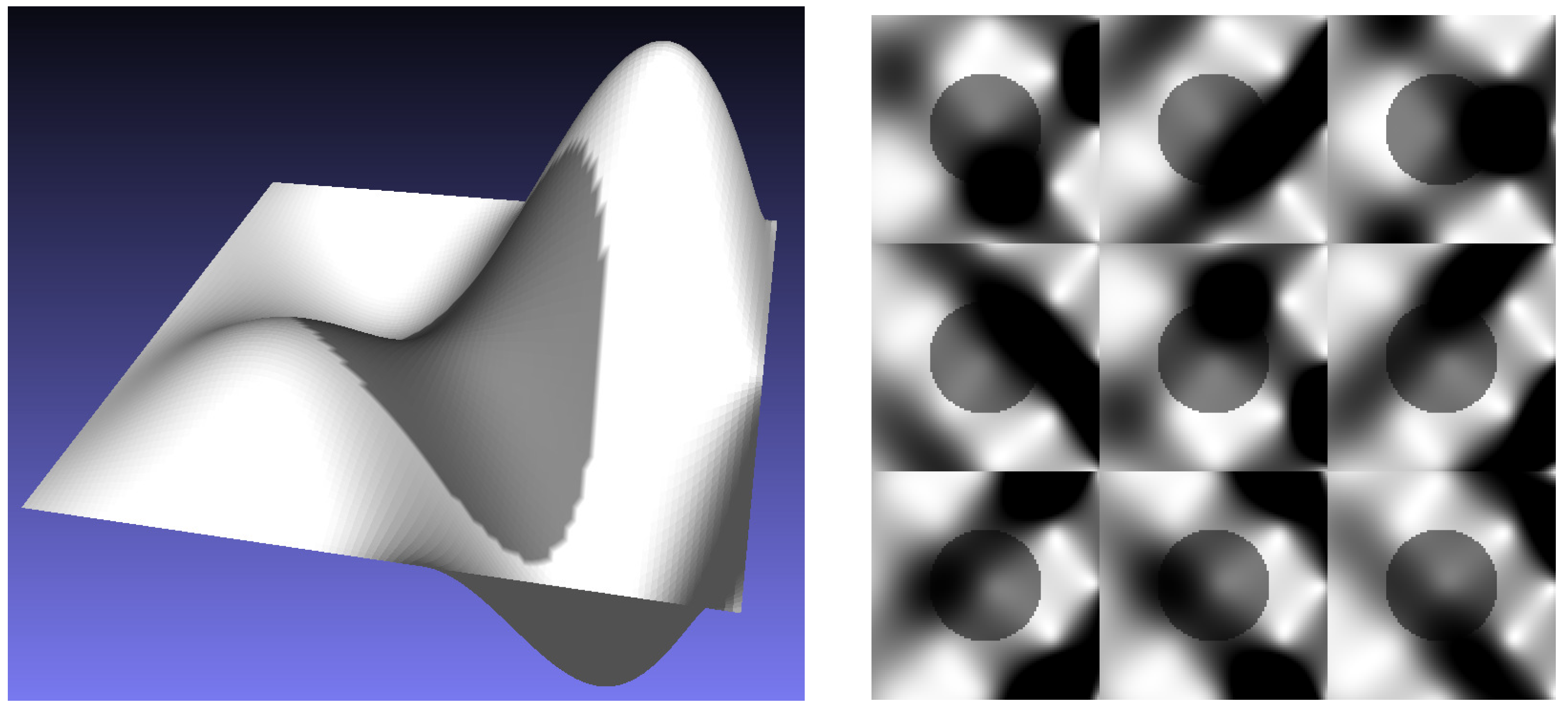
We initially apply the two methods to a synthetic dataset, first considered in [15]. The analytical expression $z=u(x,y)$ of the observed surface, displayed in the left-hand pane of Figure 3, is fixed a priori, and a simple white and gray image is texture mapped to it. The synthetic images are obtained by applying the PS forward model to the surface. The images displayed on the right of Figure 3 were produced by choosing a set of nine lighting directions. In this case, the light sources were located at an infinite distance from the target, but the model allows choosing the lighting distance using the width A of the domain $\mathrm{\Omega }$ (see (1)) as a unit of measure.

We used the dataset reported in Figure 3, with lights at infinity and no noise, substituting the third image with one obtained with a light source at distance $\delta A$, for $\delta =10,8,6,4,2$. We also contaminated this image with Gaussian noise having mean value zero and standard deviation $0.1$. This produces a dataset where the only unideal image is the number 3.

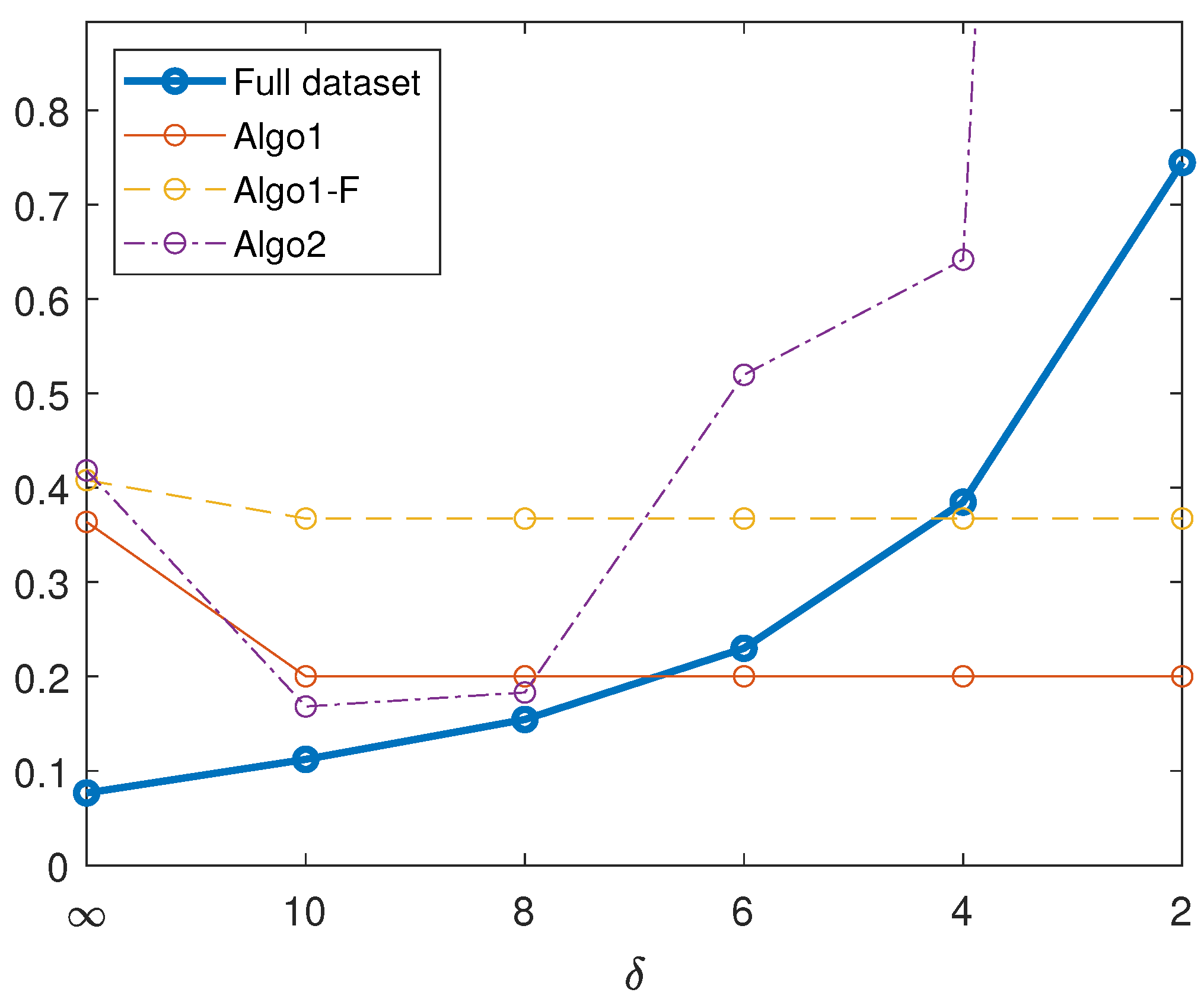
The blue thick line in Figure 4 represents the relative error

$$E\left(\delta \right)=\frac{\parallel u(x,y)-\tilde{u}{(x,y)\parallel }_{\infty }}{{\parallel u(x,y)\parallel }_{\infty }},$$

where ${\parallel u(x,y)\parallel }_{\infty }={max}_{(x,y)\in \mathrm{\Omega }}\left|u(x,y)\right|$, $u(x,y)$ is the model surface, and $\tilde{u}(x,y)$ is the reconstruction obtained by processing the whole dataset, where the third light source is at distance $\delta A$. The other three lines represent the error obtained by processing a reduced dataset, according to the recommendation of Algorithm 1 (Algo1), the fast version of the same method (Algo1-F), and Algorithm 2 (Algo2).

It can be seen that, while the error corresponding to the whole dataset increases as $\delta$ decreases, the two versions of Algorithm 1 identify a subset for which the error is reduced, when the light source is very close. Indeed, both versions select Image 3 as the first to be removed, while the fast version (incorrectly) also excludes Image 1 from the dataset. On the contrary, Algorithm 2 fails, as it excludes Images 5 and 6, leading to a larger error. The fast version of Algorithm 2 leads to even worse results.

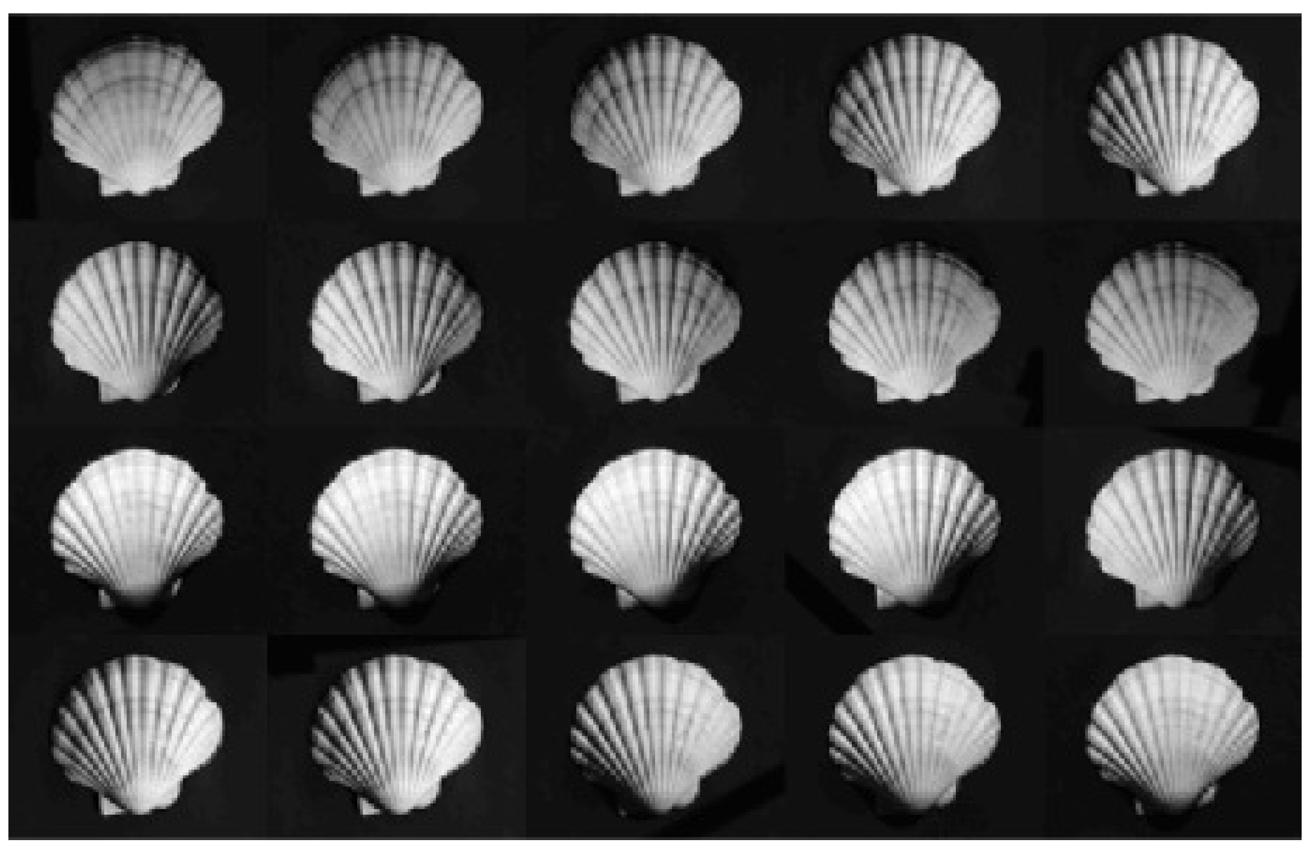
While the first experiment was concerned with the case of a perfect Lambertian reflector illuminated by a close light source, in the second one we investigate the case of a non-Lambertian surface with lights at almost infinite distance from it. The Shell3 dataset, displayed in Figure 5, was used for the first time in [20]. A preliminary version of the dataset has been considered in [15]. The pictures were obtained by placing a seashell, approximately 10 cm wide, on a rotating platform in the open air. The same platform holds a tripod with a camera observing the shell from above, at a distance of about 1 m (see [20]). Twenty images were taken by letting the platform rotate clockwise under direct sunlight.

The relatively large distance between the camera and the shell, coupled with a lens with a focal length of 85 mm, produces a reasonable approximation of an orthographic projection. The light source is virtually at an infinite distance from the object. Nevertheless, the Hayakawa procedure fails when it is applied to the whole dataset, as in this case the matrix G in (7) is not positive definite. This is probably due to the fact that the shell surface does not reflect the light according to Lambert’s law.

We report in the following the indices of the images that were excluded from the dataset, after processing the data matrix M of size 702,927 × 20, by each of the four methods discussed in Section 4:

Algorithm 1:

 3, 13, 2;

Algorithm 1-fast version:

 3, 13, 2, 17, 20, 5, 11;

Algorithm 2:

 3, 20, 7, 2;

Algorithm 2-fast version:

 3, 20, 5.

Each of the four lines contains the ordered list of the images identified at each iteration of Algorithms 1 (Line 24) and 2 (Line 22). Each list is terminated when the stop condition of the main loop is met (Lines 34 and 25, respectively).

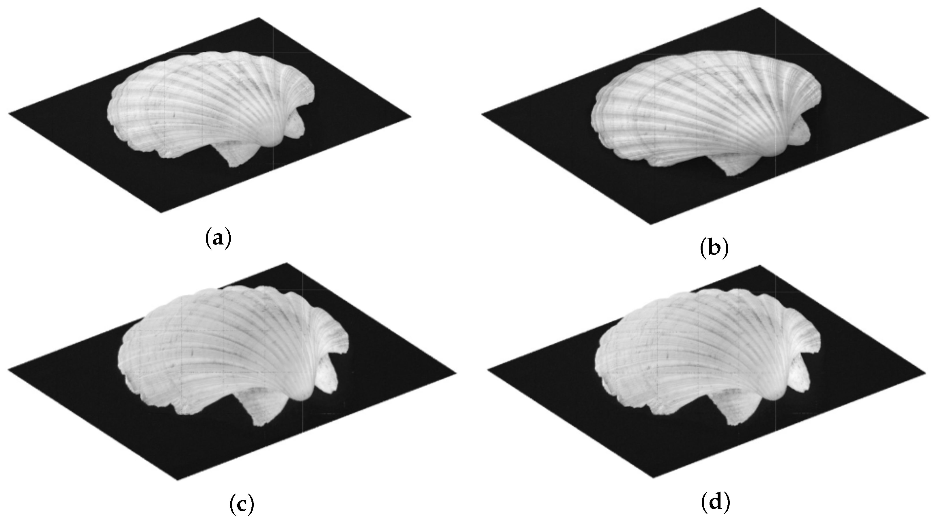
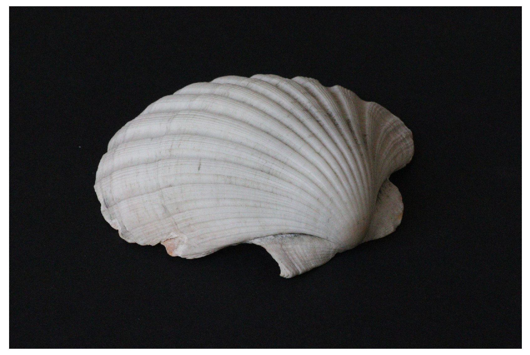
Figure 6 reports a view of the reconstructions obtained by the four methods. They should be compared with the picture of the real seashell, displayed in Figure 7. Even if in this case it is not possible to obtain a numerical measure of the error, it is evident that the surfaces recovered by Algorithm 2 are much closer to the original, while those produced by Algorithm 1 are considerably flatter.

6. Discussion

Our numerical experiments faced two situations of particular importance in PS. In the first one, all the images in the synthetic dataset meet the assumptions of the PS model, except for one image, which represents the same Lambertian surface lighted by a source approaching the target and is affected by $10\%$ Gaussian noise.

As Figure 4 shows, while processing the whole dataset leads to an error that increases as the light source approaches the surface, Algorithm 1 is able to identify the disturbing image, and its removal leads to a substantial reduction in the error. The fast version of the same method proves to be less accurate, but still produces a smaller error than the unreduced dataset. Algorithm 2, on the contrary, is not able to select the unideal image, and selects a subset that degrades the quality of the reconstruction.

Figure 4 also shows that for $\delta \ge 8$ the error in the reconstruction is not much larger than with a light source at infinity, and removing the single unideal image from the dataset produces slightly worse results. The quality of the recovered surface is strongly affected by a close light source only when $\delta \le 4$, that is, in very narrow shooting scenarios.

The second dataset is experimental and it is correctly illuminated, since the sunlight produces practically parallel rays. Anyway, the surface of the seashell is probably not Lambertian, and the pictures are affected by measuring errors. The standard Hayakawa procedure is not applicable to the dataset, as it breaks when computing the Cholesky factorization of G in (7), so the dataset must be reduced. We see that both developed algorithms are able to produce a meaningful solution, but the reconstruction produced by Algorithm 2 seems to better approximate the original seashell, even when the fast version of the method is employed. These results are in contrast with the graph in Figure 4, which reports the error behavior for the synthetic dataset, where Algorithm 1 performs better.

The above consideration suggests that both methods may have a role in detecting a lack of ideality in a large dataset, with regard to the presence of close light sources and of a non-Lambertian target. Our further studies will address the development of a procedure that blends the two approaches for analyzing a redundant dataset. An immediate advantage of the two algorithms is that they suggest an ordered list of pictures to be excluded from the numerical computation, which may assist the user in preprocessing a dataset to better suit their needs. This may be accomplished by visually comparing the reconstructed surfaces to the true object. Indeed, the computing time required by the algorithms proposed in this paper to reduce the dataset, and by the package presented in [15] to generate the reconstructions, allows for fast on-site processing on a laptop.

To conclude, the proposed new approaches look promising for determining a subset of an experimental PS dataset that better approximates the strict assumptions required by Lambert’s model under unknown lighting. One of their limitations is that they always exclude at least one picture from the initial dataset, even if it is a perfect one. This means that they are not able to evaluate a dataset in itself, but only to compare successive subsets of the initial collection of images, and that their application must always be supervised by a human operator. We believe that a hybrid method, which keeps into account the forecasts of both algorithms, may improve their performance, but this requires more work. What is also needed is a wide experimentation on well-known collections of PS data, such as [32,33], as well as on images acquired in less restrictive conditions than the ones considered in this paper, to compare the performance of the proposed methods to other available techniques. This will be the subject of future research.