A State of the Art Review of Systems of Linear Inequalities and Related Observability Problems

Abstract

This work is a short review of the state of the art aiming to contribute to the use, disclosure, and propagation of systems of linear inequalities in real life, teaching, and research. It shows that the algebraic structure of their solutions consists of the sum of a linear subspace, an acute cone, and a polytope, and that adequate software exists to obtain, in their simplest forms, these three components. The work describes, based on orthogonality and polarity, homogeneous and complete systems of inequalities, the associated compatibility problems, and their relations with convex polyhedra and polytopes, which are the only possible solution for bounded problems, the most common in real practice. The compatibility and the observability problems, including their symbolic forms, are analyzed and solved, identifying the subsets of unknowns with unique solutions and those unbounded, important items of information with practical relevance in artificial intelligence and automatic learning. Having infinitely many solutions of a given problem allows us to find solutions when some of the assumptions fail and unexpected constraints come into play, a common situation for engineers. The linear programming problem becomes trivial when the set of all solutions is available and all solutions are obtained, contrary to the case of standard programs that provide only one solution. Several examples of applications to several areas of knowledge are presented, illustrating the advantages of solving these systems of inequalities.

1. Introduction and Motivation

Linear systems of inequalities appear very frequently and play a central role in real practice. Cases of special relevance are those of linear programming problems, but there are many more. However, in spite of their importance, the way of dealing with these systems of equations is not well known and has not reached sufficiently the group of people working with these problems and their applications. In addition, the software available to solve them is not easily available and most people ignore where to find it. Consequently, this field has not advanced as expected. It is frustrating to enter the internet and look for methods to solve these systems and, incomprehensibly, find lots of entries in which only the cases of one, two or, at most, three inequalities are dealt with, giving the impression that general methods for large systems do not exist, when this is not the case. Some available software for small problems can be downloaded from: (https://meteo.unican.es/temp/castie/GammaAlgorithm/GammaAlgorithm.zip, accessed on 12 July 2023).

In addition, the problem of the solution of these systems has not been connected sufficiently with their associated problems in other fields, in which important advances were produced a ong time ago. This is the case of identifying the main components of polyhedra, such as edges, vertices, and facets, together with the methods to obtain then numerically (see [1], who finds the convex hull, facet by facet, and [2], who provide a pivoting algorithm to obtain facets and vertices). Since most linear systems of inequalities arising in real practice problems are bounded, that is, their sets of solutions are polytopes generated by their vertices, and methods for finding the vertices of a polytope are well known (e.g., [2,3] or [4]), they should be used very frequently to solve them. Unfortunately, this is not the case. If one looks at the less frequent case of unbounded problems, similar conclusions can be drawn.

Due to its connection with linear programming, some methods to solve systems of linear inequalities have been based on this problem, as, for example, the one described in [5], which solves only some particular cases.

In this paper, concerned with this fact and trying to break with this undesirable situation, we deal with a summary of the state of the art of these systems of inequalities and review some of the existing work, including some illustrative examples to motivate users and researchers to use these relevant tools and to facilitate and make available these important tools to people.

The paper is organized as follows. In Section 2, linear systems of equations are discussed with special consideration to their compatibility conditions and the identification of the subsets of unknowns that are unbounded or have unique solutions. In Section 3, we analyze systems of linear inequalities, homogeneous and complete, together with their corresponding compatibility problems, which become more complex than the case of systems of linear equations, because here dual cones replace orthogonal subspaces. In Section 4, the observability problem is presented and analyzed. We will see that between the two extremes of incompatibility and whole observability there is an interesting range of partial observability cases, which have important applications. In systems of linear inequalities in which there are infinitely many solutions, some set of unknowns could be uniquely identified, and for those with multiple solutions, lower and upper bounds and several other interesting items of information can be easily obtained. In Section 5, we demonstrate that the problem of linear programming becomes trivial if the system of constraints is initially solved or stated directly in its polyhedral form. Next, in Section 6, we present some examples of applications to motivate the use of the tools mentioned in this paper. Finally, we end, in Section 7, with a set of conclusions, as a summary of the paper’s contributions.

2. Systems of Linear Equations

The simplest and degenerated example of a system of linear inequalities is the system of linear equations, in which case the inequalities convert into equalities. The problem of analyzing the compatibility of these systems and solving them, obtaining their general solutions, i.e., all possible solutions, has important applications in practice. Apart from this work, the interested reader can find a free course at: https://www.uclm.es/Conocimiento/Cursos/Algebra-1-En, accessed on 12 July 2023.

2.1. Homogeneous Systems of Linear Equations

Consider first the interesting particular case of the homogeneous case (https://www.uclm.es/Conocimiento/Cursos/Algebra-1-En/Bloque-3/Item-9?id_peticion=DE2DCBDB-4EAD-4030-9E2F-F705FC2CDF76, accessed on 12 July 2023), in which all the b coefficients are null, that is,

$$\begin{array}{ccc}{a}_{11}{x}_1+a_{12}{x}_2+\dots +a_{1n}{x}_n& =& 0\\ a_{21}{x}_1+a_{22}{x}_2+\dots +a_{2n}{x}_n& =& 0\\ \cdots \cdots \cdots \cdots \cdots \cdots \\ a_{m1}{x}_1+a_{m2}{x}_2+\cdots +a_{mn}{x}_n& =& 0,\end{array}$$

(1)

which, from the point of view of orthogonality, can be written in the equivalent form as:

$$\begin{array}{ccc}(a_{11},a_{12},\cdots ,a_{1n})·(x_1,x_2,\cdots ,x_n)& =& 0\\ (a_{21},a_{22},\cdots ,a_{2n})·(x_1,x_2,\cdots ,x_n)& =& 0\\ \cdots \cdots \cdots \cdots \cdots \cdots \cdots \cdots \cdots \cdots \cdots & \cdots & \\ (a_{m1},a_{m2},\cdots ,a_{mn})·(x_1,x_2,\cdots ,x_n)& =& 0.\end{array}$$

(2)

Since the above dot products are null, which implies orthogonality, this view allows us to conclude immediately that the set of solutions of the homogeneous system is the orthogonal subspace of the subspace generated by the vectors of coefficients of the different equations.

2.2. Complete Systems of Linear Equations

Next, consider the complete linear system of equations (https://www.uclm.es/Conocimiento/Cursos/Algebra-1-En/Bloque-3/Item-10?id_peticion=DE2DCBDB-4EAD-4030-9E2F-F705FC2CDF76, accessed on 12 July 2023):

$$\begin{array}{cccccc}{a}_{11}{x}_1& +a_{12}{x}_2& +\cdots & +a_{1n}{x}_n& =& b_1\\ a_{21}{x}_1& +a_{22}{x}_2& +\cdots & +a_{2n}{x}_n& =& b_2\\ \cdots & \cdots & \cdots & \cdots & \cdots & \cdots \\ a_{m1}{x}_1& +a_{m2}{x}_2& +\cdots & +a_{mn}{x}_n& =& b_m,\end{array}$$

(3)

where not all b coefficients are zeros.

For the orthogonal subspace to appear somewhere, we write this system in an equivalent form. To this end, first, we multiply the right-hand side terms, $b_1,b_2,\dots ,b_m$, by a virtual unknown $x_{n+1}$, which we make equal to 1 in order not to alter the system. Thus, we add the last constraint $x_{n+1}=1$ and move all $x_{n+1}$ terms to the left-hand sides to obtain:

$$\begin{array}{ccccccc}{a}_{11}{x}_1& +a_{12}{x}_2& +\cdots & +a_{1n}{x}_n& -b_1{x}_{n+1}& =& 0\\ a_{21}{x}_1& +a_{22}{x}_2& +\cdots & +a_{2n}{x}_n& -b_2{x}_{n+1}& =& 0\\ \cdots & \cdots & \cdots & \cdots & \cdots & \cdots & \cdots \\ a_{m1}{x}_1& +a_{m2}{x}_2& +\cdots & +a_{mn}{x}_n& -b_m{x}_{n+1}& =& 0\\ & & & & x_{n+1}& =& 1.\end{array}$$

(4)

Next, we solve the homogeneous system and later impose the constraint $x_{n+1}=1$ and remove this virtual constraint from the solution.

It is well known that the general solution we obtain, if it exists, is the sum of a linear subspace plus a particular solution, that is, an affine space.

If the system is homogeneous, that is, all the independent terms are null, the solution, if not degenerated, is a linear subspace and then it is unbounded. Thus, the only bounded case requires the non-existence of the linear subspace part in the solution. In addition, the bounded solutions are always unique.

An algorithm to obtain the orthogonal subspace of a given linear subspace can be seen in [6]. Based on the orthogonality concept the algorithm has very interesting applications, such as calculating and updating inverses and determinants, solving linear systems of equations and analyzing their compatibility, etc.

It is interesting to see the case of linear systems of equations from the point of view of orthogonality as above. In fact, it has been shown that the set of solutions of a homogeneous system is the linear subspace orthogonal to the linear subspace generated by the equation coefficients. This will become even more interesting when we analyze the general problem of linear systems of inequalities from the point of view of duality, where we will see that the dual cone of a linear subspace is its orthogonal subspace. Consequently, we will discover that the concept of dual cone is an extension of the concept of orthogonal subspace.

We recommend to the readers the convenience of handling different points of view, which will allow them to solve problems and guess their solutions more directly and in some cases solve them immediately. For example, the problem of determining whether or not a vector belongs to a linear subspace or the problem of obtaining the intersection of two linear subspaces can be solved taking into account the equivalences in

Table 1. Important equivalences from the point of view of orthogonality.

Three ways of checking if a vector belongs to a linear subspace

$v\in \mathcal{L}(a_1,a_2,\cdots ,a_n)\iff v\in {\left(\mathcal{L}{(a_1,a_2,\cdots ,a_n)}^{\perp }\right)}^{\perp }\iff v\perp \mathcal{L}{(a_1,a_2,\cdots ,a_n)}^{\perp }$

Three ways of obtaining the intersection of two subspaces

$S_1\bigcap S_2\iff S_1\bigcap {\left(S_2^{\perp }\right)}^{\perp }\iff {\left(S_1^{\perp }\right)}^{\perp }\bigcap S_2$

.

In fact, to see if the vector v belongs to the linear subspace $\mathcal{L}(a_1,a_2,\dots ,a_n)$, we obtain first the orthogonal subspace $\mathcal{L}{(a_1,a_2,\dots ,a_n)}^{\perp }$ and then we check that the dot products of v and its generators are all null.

Similarly, to obtain the intersection $S_1\bigcap S_2$ of two linear subspaces $S_1$ and $S_2$, we first obtain the orthogonal subspace $S_1^{\perp }$ and later the orthogonal subspace ${\left(S_1^{\perp }\right)}^{\perp }$ of $S_1^{\perp }$ in $S_2$. Then, it is evident that the ways of solving these two problems come from our new point of view.

The Plate Scanning Example

In this section, we illustrate the proposed methods by their application to a simple example. The reader can find another example in [7]. Consider the traffic network in Figure 1, which contains six nodes and nine links, and consider the origin–destination nodes (OD) and the nine routes indicated in

Table 2. Data for the simple example, including OD pairs, routes, links, scanned information, and observed scanned flows w.

OD	Route Number (r)	Links				$\mathit{r}\bigcap \mathbf{SC}$	w
1-3	1	1	2			{1}	$w_1$
1-6	2	1	5	6		{1,5,6}	$w_2$
2-3	3	2				-	-
2-3	3	5	8			{5,8}	$w_3$
2-5	4	5				{5}	$w_4$
2-6	5	5	6			{5,6}	$w_5$
3-1	6	9				{9}	$w_6$
3-2	7	9	1			{1,9}	$w_7$
4-5	8	4	1	5		{1,4,5}	$w_8$
5-1	9	8	9			{8,9}	$w_9$
5-1	9	6	7	3	4	{4,6}	$w_{10}$
5-1	9	6	7	9		{6,9}	$w_{11}$

, where its third column contains all route links.

In order to obtain information about the circulating traffic, we scan the plate numbers of the vehicles passing by links $1,4,5,6,8,9$, that is, our set of scanned links is the set $\mathit{SC}=\{1,4,5,6,8,9\}$. Table 2, in its fourth column, contains the scanned links of each route, and in its last column the number of scanned vehicles associated with each route. For example, $w_1$ is the number of scanned vehicles only in the camera of link 1, and $w_2$ is the number of vehicles scanned in the three links 1, 5, and 6. Note that this can be achieved thanks to the vehicle plate numbers.

We look for the sets of links, OD pairs, and route flows that are observable, that is, whose flows can be calculated in terms of the flows $\{w_1,w_2,\cdots ,w_{11}\}$.

If, with the help of Table 2, we write the links, OD pairs, and scanned flows in terms of the route flows, we obtain the following system of equations:

$$\left(\begin{array}{c}{v}_1\\ v_2\\ v_3\\ v_4\\ v_5\\ v_6\\ v_7\\ v_8\\ v_9\\ -\\ t_1\\ t_2\\ t_3\\ t_4\\ t_5\\ t_6\\ t_7\\ t_8\\ t_9\\ -\\ w_1\\ w_2\\ w_3\\ w_4\\ w_5\\ w_6\\ w_7\\ w_8\\ w_9\\ w_{10}\\ w_{11}\end{array}\right)=\left(\begin{array}{cccccccccccc}\hfill 1& \hfill 1& \hfill 0& \hfill 0& \hfill 0& \hfill 0& \hfill 0& \hfill 1& \hfill 1& \hfill 0& \hfill 0& \hfill 0\\ \hfill 1& \hfill 0& \hfill 1& \hfill 0& \hfill 0& \hfill 0& \hfill 0& \hfill 0& \hfill 0& \hfill 0& \hfill 0& \hfill 0\\ \hfill 0& \hfill 0& \hfill 0& \hfill 0& \hfill 0& \hfill 0& \hfill 0& \hfill 0& \hfill 0& \hfill 0& \hfill 1& \hfill 0\\ \hfill 0& \hfill 0& \hfill 0& \hfill 0& \hfill 0& \hfill 0& \hfill 0& \hfill 0& \hfill 1& \hfill 0& \hfill 1& \hfill 0\\ \hfill 0& \hfill 1& \hfill 0& \hfill 1& \hfill 1& \hfill 1& \hfill 0& \hfill 0& \hfill 1& \hfill 0& \hfill 0& \hfill 0\\ \hfill 0& \hfill 1& \hfill 0& \hfill 0& \hfill 0& \hfill 1& \hfill 0& \hfill 0& \hfill 0& \hfill 0& \hfill 1& \hfill 1\\ \hfill 0& \hfill 0& \hfill 0& \hfill 0& \hfill 0& \hfill 0& \hfill 0& \hfill 0& \hfill 0& \hfill 0& \hfill 1& \hfill 1\\ \hfill 0& \hfill 0& \hfill 0& \hfill 1& \hfill 0& \hfill 0& \hfill 0& \hfill 0& \hfill 0& \hfill 1& \hfill 0& \hfill 0\\ \hfill 0& \hfill 0& \hfill 0& \hfill 0& \hfill 0& \hfill 0& \hfill 1& \hfill 1& \hfill 0& \hfill 1& \hfill 0& \hfill 1\\ \hfill -& \hfill -& \hfill -& \hfill -& \hfill -& \hfill -& \hfill -& \hfill -& \hfill -& \hfill -& \hfill -& \hfill -\\ \hfill 1& \hfill 0& \hfill 0& \hfill 0& \hfill 0& \hfill 0& \hfill 0& \hfill 0& \hfill 0& \hfill 0& \hfill 0& \hfill 0\\ \hfill 0& \hfill 1& \hfill 0& \hfill 0& \hfill 0& \hfill 0& \hfill 0& \hfill 0& \hfill 0& \hfill 0& \hfill 0& \hfill 0\\ \hfill 0& \hfill 0& \hfill 1& \hfill 1& \hfill 0& \hfill 0& \hfill 0& \hfill 0& \hfill 0& \hfill 0& \hfill 0& \hfill 0\\ \hfill 0& \hfill 0& \hfill 0& \hfill 0& \hfill 1& \hfill 0& \hfill 0& \hfill 0& \hfill 0& \hfill 0& \hfill 0& \hfill 0\\ \hfill 0& \hfill 0& \hfill 0& \hfill 0& \hfill 0& \hfill 1& \hfill 0& \hfill 0& \hfill 0& \hfill 0& \hfill 0& \hfill 0\\ \hfill 0& \hfill 0& \hfill 0& \hfill 0& \hfill 0& \hfill 0& \hfill 1& \hfill 0& \hfill 0& \hfill 0& \hfill 0& \hfill 0\\ \hfill 0& \hfill 0& \hfill 0& \hfill 0& \hfill 0& \hfill 0& \hfill 0& \hfill 1& \hfill 0& \hfill 0& \hfill 0& \hfill 0\\ \hfill 0& \hfill 0& \hfill 0& \hfill 0& \hfill 0& \hfill 0& \hfill 0& \hfill 0& \hfill 1& \hfill 0& \hfill 0& \hfill 0\\ \hfill 0& \hfill 0& \hfill 0& \hfill 0& \hfill 0& \hfill 0& \hfill 0& \hfill 0& \hfill 0& \hfill 1& \hfill 1& \hfill 1\\ \hfill -& \hfill -& \hfill -& \hfill -& \hfill -& \hfill -& \hfill -& \hfill -& \hfill -& \hfill -& \hfill -& \hfill -\\ \hfill 1& \hfill 0& \hfill 0& \hfill 0& \hfill 0& \hfill 0& \hfill 0& \hfill 0& \hfill 0& \hfill 0& \hfill 0& \hfill 0\\ \hfill 0& \hfill 1& \hfill 0& \hfill 0& \hfill 0& \hfill 0& \hfill 0& \hfill 0& \hfill 0& \hfill 0& \hfill 0& \hfill 0\\ \hfill 0& \hfill 0& \hfill 0& \hfill 1& \hfill 0& \hfill 0& \hfill 0& \hfill 0& \hfill 0& \hfill 0& \hfill 0& \hfill 0\\ \hfill 0& \hfill 0& \hfill 0& \hfill 0& \hfill 1& \hfill 0& \hfill 0& \hfill 0& \hfill 0& \hfill 0& \hfill 0& \hfill 0\\ \hfill 0& \hfill 0& \hfill 0& \hfill 0& \hfill 0& \hfill 1& \hfill 0& \hfill 0& \hfill 0& \hfill 0& \hfill 0& \hfill 0\\ \hfill 0& \hfill 0& \hfill 0& \hfill 0& \hfill 0& \hfill 0& \hfill 1& \hfill 0& \hfill 0& \hfill 0& \hfill 0& \hfill 0\\ \hfill 0& \hfill 0& \hfill 0& \hfill 0& \hfill 0& \hfill 0& \hfill 0& \hfill 1& \hfill 0& \hfill 0& \hfill 0& \hfill 0\\ \hfill 0& \hfill 0& \hfill 0& \hfill 0& \hfill 0& \hfill 0& \hfill 0& \hfill 0& \hfill 1& \hfill 0& \hfill 0& \hfill 0\\ \hfill 0& \hfill 0& \hfill 0& \hfill 0& \hfill 0& \hfill 0& \hfill 0& \hfill 0& \hfill 0& \hfill 1& \hfill 0& \hfill 0\\ \hfill 0& \hfill 0& \hfill 0& \hfill 0& \hfill 0& \hfill 0& \hfill 0& \hfill 0& \hfill 0& \hfill 0& \hfill 1& \hfill 0\\ \hfill 0& \hfill 0& \hfill 0& \hfill 0& \hfill 0& \hfill 0& \hfill 0& \hfill 0& \hfill 0& \hfill 0& \hfill 0& \hfill 1\end{array}\right)\left(\begin{array}{c}{r}_1\\ r_2\\ r_3\\ r_4\\ r_5\\ r_6\\ r_7\\ r_8\\ r_9\\ r_{10}\\ r_{11}\\ r_{12}\end{array}\right)$$

(5)

where $\mathbf{v},\mathbf{t},\mathbf{w}$, and $\mathbf{r}$ are the vectors of route, link, OD pairs, and plate scanned flows, respectively.

Since the data in this case consists of the scanned flows $w_1$ to $w_{11}$, we can rearrange this system (5) in the form:

$$\left(\begin{array}{cccccccccccccccccccccccccccccccc}\hfill 1& \hfill 1& \hfill 0& \hfill 0& \hfill 0& \hfill 0& \hfill 0& \hfill 1& \hfill 1& \hfill 0& \hfill 0& \hfill 0& \hfill |& \hfill -1& \hfill 0& \hfill 0& \hfill 0& \hfill 0& \hfill 0& \hfill 0& \hfill 0& \hfill 0& \hfill |& \hfill 0& \hfill 0& \hfill 0& \hfill 0& \hfill 0& \hfill 0& \hfill 0& \hfill 0& \hfill 0\\ \hfill 1& \hfill 0& \hfill 1& \hfill 0& \hfill 0& \hfill 0& \hfill 0& \hfill 0& \hfill 0& \hfill 0& \hfill 0& \hfill 0& \hfill |& \hfill 0& \hfill -1& \hfill 0& \hfill 0& \hfill 0& \hfill 0& \hfill 0& \hfill 0& \hfill 0& \hfill |& \hfill 0& \hfill 0& \hfill 0& \hfill 0& \hfill 0& \hfill 0& \hfill 0& \hfill 0& \hfill 0\\ \hfill 0& \hfill 0& \hfill 0& \hfill 0& \hfill 0& \hfill 0& \hfill 0& \hfill 0& \hfill 0& \hfill 0& \hfill 1& \hfill 0& \hfill |& \hfill 0& \hfill 0& \hfill -1& \hfill 0& \hfill 0& \hfill 0& \hfill 0& \hfill 0& \hfill 0& \hfill |& \hfill 0& \hfill 0& \hfill 0& \hfill 0& \hfill 0& \hfill 0& \hfill 0& \hfill 0& \hfill 0\\ \hfill 0& \hfill 0& \hfill 0& \hfill 0& \hfill 0& \hfill 0& \hfill 0& \hfill 0& \hfill 1& \hfill 0& \hfill 1& \hfill 0& \hfill |& \hfill 0& \hfill 0& \hfill 0& \hfill -1& \hfill 0& \hfill 0& \hfill 0& \hfill 0& \hfill 0& \hfill |& \hfill 0& \hfill 0& \hfill 0& \hfill 0& \hfill 0& \hfill 0& \hfill 0& \hfill 0& \hfill 0\\ \hfill 0& \hfill 1& \hfill 0& \hfill 1& \hfill 1& \hfill 1& \hfill 0& \hfill 0& \hfill 1& \hfill 0& \hfill 0& \hfill 0& \hfill |& \hfill 0& \hfill 0& \hfill 0& \hfill 0& \hfill -1& \hfill 0& \hfill 0& \hfill 0& \hfill 0& \hfill |& \hfill 0& \hfill 0& \hfill 0& \hfill 0& \hfill 0& \hfill 0& \hfill 0& \hfill 0& \hfill 0\\ \hfill 0& \hfill 1& \hfill 0& \hfill 0& \hfill 0& \hfill 1& \hfill 0& \hfill 0& \hfill 0& \hfill 0& \hfill 1& \hfill 1& \hfill |& \hfill 0& \hfill 0& \hfill 0& \hfill 0& \hfill 0& \hfill -1& \hfill 0& \hfill 0& \hfill 0& \hfill |& \hfill 0& \hfill 0& \hfill 0& \hfill 0& \hfill 0& \hfill 0& \hfill 0& \hfill 0& \hfill 0\\ \hfill 0& \hfill 0& \hfill 0& \hfill 0& \hfill 0& \hfill 0& \hfill 0& \hfill 0& \hfill 0& \hfill 0& \hfill 1& \hfill 1& \hfill |& \hfill 0& \hfill 0& \hfill 0& \hfill 0& \hfill 0& \hfill 0& \hfill -1& \hfill 0& \hfill 0& \hfill |& \hfill 0& \hfill 0& \hfill 0& \hfill 0& \hfill 0& \hfill 0& \hfill 0& \hfill 0& \hfill 0\\ \hfill 0& \hfill 0& \hfill 0& \hfill 1& \hfill 0& \hfill 0& \hfill 0& \hfill 0& \hfill 0& \hfill 1& \hfill 0& \hfill 0& \hfill |& \hfill 0& \hfill 0& \hfill 0& \hfill 0& \hfill 0& \hfill 0& \hfill 0& \hfill -1& \hfill 0& \hfill |& \hfill 0& \hfill 0& \hfill 0& \hfill 0& \hfill 0& \hfill 0& \hfill 0& \hfill 0& \hfill 0\\ \hfill 0& \hfill 0& \hfill 0& \hfill 0& \hfill 0& \hfill 0& \hfill 1& \hfill 1& \hfill 0& \hfill 1& \hfill 0& \hfill 1& \hfill |& \hfill 0& \hfill 0& \hfill 0& \hfill 0& \hfill 0& \hfill 0& \hfill 0& \hfill 0& \hfill -1& \hfill |& \hfill 0& \hfill 0& \hfill 0& \hfill 0& \hfill 0& \hfill 0& \hfill 0& \hfill 0& \hfill 0\\ \hfill -& \hfill -& \hfill -& \hfill -& \hfill -& \hfill -& \hfill -& \hfill -& \hfill -& \hfill -& \hfill -& \hfill -& \hfill -& \hfill -& \hfill -& \hfill -& \hfill -& \hfill -& \hfill -& \hfill -& \hfill -& \hfill -& \hfill -& \hfill -& \hfill -& \hfill -& \hfill -& \hfill -& \hfill -& \hfill -& \hfill -& \hfill -\\ \hfill 1& \hfill 0& \hfill 0& \hfill 0& \hfill 0& \hfill 0& \hfill 0& \hfill 0& \hfill 0& \hfill 0& \hfill 0& \hfill 0& \hfill |& \hfill 0& \hfill 0& \hfill 0& \hfill 0& \hfill 0& \hfill 0& \hfill 0& \hfill 0& \hfill 0& \hfill |& \hfill -1& \hfill 0& \hfill 0& \hfill 0& \hfill 0& \hfill 0& \hfill 0& \hfill 0& \hfill 0\\ \hfill 0& \hfill 1& \hfill 0& \hfill 0& \hfill 0& \hfill 0& \hfill 0& \hfill 0& \hfill 0& \hfill 0& \hfill 0& \hfill 0& \hfill |& \hfill 0& \hfill 0& \hfill 0& \hfill 0& \hfill 0& \hfill 0& \hfill 0& \hfill 0& \hfill 0& \hfill |& \hfill 0& \hfill -1& \hfill 0& \hfill 0& \hfill 0& \hfill 0& \hfill 0& \hfill 0& \hfill 0\\ \hfill 0& \hfill 0& \hfill 1& \hfill 1& \hfill 0& \hfill 0& \hfill 0& \hfill 0& \hfill 0& \hfill 0& \hfill 0& \hfill 0& \hfill |& \hfill 0& \hfill 0& \hfill 0& \hfill 0& \hfill 0& \hfill 0& \hfill 0& \hfill 0& \hfill 0& \hfill |& \hfill 0& \hfill 0& \hfill -1& \hfill 0& \hfill 0& \hfill 0& \hfill 0& \hfill 0& \hfill 0\\ \hfill 0& \hfill 0& \hfill 0& \hfill 0& \hfill 1& \hfill 0& \hfill 0& \hfill 0& \hfill 0& \hfill 0& \hfill 0& \hfill 0& \hfill |& \hfill 0& \hfill 0& \hfill 0& \hfill 0& \hfill 0& \hfill 0& \hfill 0& \hfill 0& \hfill 0& \hfill |& \hfill 0& \hfill 0& \hfill 0& \hfill -1& \hfill 0& \hfill 0& \hfill 0& \hfill 0& \hfill 0\\ \hfill 0& \hfill 0& \hfill 0& \hfill 0& \hfill 0& \hfill 1& \hfill 0& \hfill 0& \hfill 0& \hfill 0& \hfill 0& \hfill 0& \hfill |& \hfill 0& \hfill 0& \hfill 0& \hfill 0& \hfill 0& \hfill 0& \hfill 0& \hfill 0& \hfill 0& \hfill |& \hfill 0& \hfill 0& \hfill 0& \hfill 0& \hfill -1& \hfill 0& \hfill 0& \hfill 0& \hfill 0\\ \hfill 0& \hfill 0& \hfill 0& \hfill 0& \hfill 0& \hfill 0& \hfill 1& \hfill 0& \hfill 0& \hfill 0& \hfill 0& \hfill 0& \hfill |& \hfill 0& \hfill 0& \hfill 0& \hfill 0& \hfill 0& \hfill 0& \hfill 0& \hfill 0& \hfill 0& \hfill |& \hfill 0& \hfill 0& \hfill 0& \hfill 0& \hfill 0& \hfill -1& \hfill 0& \hfill 0& \hfill 0\\ \hfill 0& \hfill 0& \hfill 0& \hfill 0& \hfill 0& \hfill 0& \hfill 0& \hfill 1& \hfill 0& \hfill 0& \hfill 0& \hfill 0& \hfill |& \hfill 0& \hfill 0& \hfill 0& \hfill 0& \hfill 0& \hfill 0& \hfill 0& \hfill 0& \hfill 0& \hfill |& \hfill 0& \hfill 0& \hfill 0& \hfill 0& \hfill 0& \hfill 0& \hfill -1& \hfill 0& \hfill 0\\ \hfill 0& \hfill 0& \hfill 0& \hfill 0& \hfill 0& \hfill 0& \hfill 0& \hfill 0& \hfill 1& \hfill 0& \hfill 0& \hfill 0& \hfill |& \hfill 0& \hfill 0& \hfill 0& \hfill 0& \hfill 0& \hfill 0& \hfill 0& \hfill 0& \hfill 0& \hfill |& \hfill 0& \hfill 0& \hfill 0& \hfill 0& \hfill 0& \hfill 0& \hfill 0& \hfill -1& \hfill 0\\ \hfill 0& \hfill 0& \hfill 0& \hfill 0& \hfill 0& \hfill 0& \hfill 0& \hfill 0& \hfill 0& \hfill 1& \hfill 1& \hfill 1& \hfill |& \hfill 0& \hfill 0& \hfill 0& \hfill 0& \hfill 0& \hfill 0& \hfill 0& \hfill 0& \hfill 0& \hfill |& \hfill 0& \hfill 0& \hfill 0& \hfill 0& \hfill 0& \hfill 0& \hfill 0& \hfill 0& \hfill -1\\ \hfill -& \hfill -& \hfill -& \hfill -& \hfill -& \hfill -& \hfill -& \hfill -& \hfill -& \hfill -& \hfill -& \hfill -& \hfill -& \hfill -& \hfill -& \hfill -& \hfill -& \hfill -& \hfill -& \hfill -& \hfill -& \hfill -& \hfill -& \hfill -& \hfill -& \hfill -& \hfill -& \hfill -& \hfill -& \hfill -& \hfill -& \hfill -\\ \hfill 1& \hfill 0& \hfill 0& \hfill 0& \hfill 0& \hfill 0& \hfill 0& \hfill 0& \hfill 0& \hfill 0& \hfill 0& \hfill 0& \hfill |& \hfill 0& \hfill 0& \hfill 0& \hfill 0& \hfill 0& \hfill 0& \hfill 0& \hfill 0& \hfill 0& \hfill |& \hfill 0& \hfill 0& \hfill 0& \hfill 0& \hfill 0& \hfill 0& \hfill 0& \hfill 0& \hfill 0\\ \hfill 0& \hfill 1& \hfill 0& \hfill 0& \hfill 0& \hfill 0& \hfill 0& \hfill 0& \hfill 0& \hfill 0& \hfill 0& \hfill 0& \hfill |& \hfill 0& \hfill 0& \hfill 0& \hfill 0& \hfill 0& \hfill 0& \hfill 0& \hfill 0& \hfill 0& \hfill |& \hfill 0& \hfill 0& \hfill 0& \hfill 0& \hfill 0& \hfill 0& \hfill 0& \hfill 0& \hfill 0\\ \hfill 0& \hfill 0& \hfill 0& \hfill 1& \hfill 0& \hfill 0& \hfill 0& \hfill 0& \hfill 0& \hfill 0& \hfill 0& \hfill 0& \hfill |& \hfill 0& \hfill 0& \hfill 0& \hfill 0& \hfill 0& \hfill 0& \hfill 0& \hfill 0& \hfill 0& \hfill |& \hfill 0& \hfill 0& \hfill 0& \hfill 0& \hfill 0& \hfill 0& \hfill 0& \hfill 0& \hfill 0\\ \hfill 0& \hfill 0& \hfill 0& \hfill 0& \hfill 1& \hfill 0& \hfill 0& \hfill 0& \hfill 0& \hfill 0& \hfill 0& \hfill 0& \hfill |& \hfill 0& \hfill 0& \hfill 0& \hfill 0& \hfill 0& \hfill 0& \hfill 0& \hfill 0& \hfill 0& \hfill |& \hfill 0& \hfill 0& \hfill 0& \hfill 0& \hfill 0& \hfill 0& \hfill 0& \hfill 0& \hfill 0\\ \hfill 0& \hfill 0& \hfill 0& \hfill 0& \hfill 0& \hfill 1& \hfill 0& \hfill 0& \hfill 0& \hfill 0& \hfill 0& \hfill 0& \hfill |& \hfill 0& \hfill 0& \hfill 0& \hfill 0& \hfill 0& \hfill 0& \hfill 0& \hfill 0& \hfill 0& \hfill |& \hfill 0& \hfill 0& \hfill 0& \hfill 0& \hfill 0& \hfill 0& \hfill 0& \hfill 0& \hfill 0\\ \hfill 0& \hfill 0& \hfill 0& \hfill 0& \hfill 0& \hfill 0& \hfill 1& \hfill 0& \hfill 0& \hfill 0& \hfill 0& \hfill 0& \hfill |& \hfill 0& \hfill 0& \hfill 0& \hfill 0& \hfill 0& \hfill 0& \hfill 0& \hfill 0& \hfill 0& \hfill |& \hfill 0& \hfill 0& \hfill 0& \hfill 0& \hfill 0& \hfill 0& \hfill 0& \hfill 0& \hfill 0\\ \hfill 0& \hfill 0& \hfill 0& \hfill 0& \hfill 0& \hfill 0& \hfill 0& \hfill 1& \hfill 0& \hfill 0& \hfill 0& \hfill 0& \hfill |& \hfill 0& \hfill 0& \hfill 0& \hfill 0& \hfill 0& \hfill 0& \hfill 0& \hfill 0& \hfill 0& \hfill |& \hfill 0& \hfill 0& \hfill 0& \hfill 0& \hfill 0& \hfill 0& \hfill 0& \hfill 0& \hfill 0\\ \hfill 0& \hfill 0& \hfill 0& \hfill 0& \hfill 0& \hfill 0& \hfill 0& \hfill 0& \hfill 1& \hfill 0& \hfill 0& \hfill 0& \hfill |& \hfill 0& \hfill 0& \hfill 0& \hfill 0& \hfill 0& \hfill 0& \hfill 0& \hfill 0& \hfill 0& \hfill |& \hfill 0& \hfill 0& \hfill 0& \hfill 0& \hfill 0& \hfill 0& \hfill 0& \hfill 0& \hfill 0\\ \hfill 0& \hfill 0& \hfill 0& \hfill 0& \hfill 0& \hfill 0& \hfill 0& \hfill 0& \hfill 0& \hfill 1& \hfill 0& \hfill 0& \hfill |& \hfill 0& \hfill 0& \hfill 0& \hfill 0& \hfill 0& \hfill 0& \hfill 0& \hfill 0& \hfill 0& \hfill |& \hfill 0& \hfill 0& \hfill 0& \hfill 0& \hfill 0& \hfill 0& \hfill 0& \hfill 0& \hfill 0\\ \hfill 0& \hfill 0& \hfill 0& \hfill 0& \hfill 0& \hfill 0& \hfill 0& \hfill 0& \hfill 0& \hfill 0& \hfill 1& \hfill 0& \hfill |& \hfill 0& \hfill 0& \hfill 0& \hfill 0& \hfill 0& \hfill 0& \hfill 0& \hfill 0& \hfill 0& \hfill |& \hfill 0& \hfill 0& \hfill 0& \hfill 0& \hfill 0& \hfill 0& \hfill 0& \hfill 0& \hfill 0\\ \hfill 0& \hfill 0& \hfill 0& \hfill 0& \hfill 0& \hfill 0& \hfill 0& \hfill 0& \hfill 0& \hfill 0& \hfill 0& \hfill 1& \hfill |& \hfill 0& \hfill 0& \hfill 0& \hfill 0& \hfill 0& \hfill 0& \hfill 0& \hfill 0& \hfill 0& \hfill |& \hfill 0& \hfill 0& \hfill 0& \hfill 0& \hfill 0& \hfill 0& \hfill 0& \hfill 0& \hfill 0\end{array}\right)\left(\begin{array}{c}{r}_1\\ r_2\\ r_3\\ r_4\\ r_5\\ r_6\\ r_7\\ r_8\\ r_9\\ r_{10}\\ r_{11}\\ r_{12}\\ -\\ v_1\\ v_2\\ v_3\\ v_4\\ v_5\\ v_6\\ v_7\\ v_8\\ v_9\\ -\\ t_1\\ t_2\\ t_3\\ t_4\\ t_5\\ t_6\\ t_7\\ t_8\\ t_9\end{array}\right)=\left(\begin{array}{c}\hfill 0\\ \hfill 0\\ \hfill 0\\ \hfill 0\\ \hfill 0\\ \hfill 0\\ \hfill 0\\ \hfill 0\\ \hfill 0\\ \hfill -\\ \hfill 0\\ \hfill 0\\ \hfill 0\\ \hfill 0\\ \hfill 0\\ \hfill 0\\ \hfill 0\\ \hfill 0\\ \hfill 0\\ \hfill -\\ \hfill 41\\ \hfill 59\\ \hfill 92\\ \hfill 65\\ \hfill 53\\ \hfill 42\\ \hfill 30\\ \hfill 25\\ \hfill 10\\ \hfill 20\\ \hfill 40\end{array}\right),$$

(6)

where the data appear as the independent terms.

Equation (6) is a system of linear equations whose matrix can be used to obtain uniquely determined flows. In fact, the generators of the linear subspace in its general solutions can be found by using the orthogonality algorithm, leading to the set of solutions:

$$\left(\begin{array}{c}{r}_1\\ r_2\\ r_3\\ r_4\\ r_5\\ r_6\\ r_7\\ r_8\\ r_9\\ r_{10}\\ r_{11}\\ r_{12}\\ -\\ v_1\\ v_2\\ v_3\\ v_4\\ v_5\\ v_6\\ v_7\\ v_8\\ v_9\\ -\\ t_1\\ t_2\\ t_3\\ t_4\\ t_5\\ t_6\\ t_7\\ t_8\\ t_9\end{array}\right)={\left(\begin{array}{c}\hfill 0\\ \hfill 0\\ \hfill 1\\ \hfill 0\\ \hfill 0\\ \hfill 0\\ \hfill 0\\ \hfill 0\\ \hfill 0\\ \hfill 0\\ \hfill 0\\ \hfill 0\\ \hfill -\\ \hfill 0\\ \hfill 1\\ \hfill 0\\ \hfill 0\\ \hfill 0\\ \hfill 0\\ \hfill 0\\ \hfill 0\\ \hfill 0\\ \hfill -\\ \hfill 0\\ \hfill 0\\ \hfill 1\\ \hfill 0\\ \hfill 0\\ \hfill 0\\ \hfill 0\\ \hfill 0\\ \hfill 0\end{array}\right)}_{\rho }+\left(\begin{array}{c}\hfill 41\\ \hfill 59\\ \hfill -92\\ \hfill 92\\ \hfill 65\\ \hfill 53\\ \hfill 42\\ \hfill 30\\ \hfill 25\\ \hfill 10\\ \hfill 20\\ \hfill 40\\ \hfill --\\ \hfill 155\\ \hfill -51\\ \hfill 20\\ \hfill 45\\ \hfill 294\\ \hfill 172\\ \hfill 60\\ \hfill 102\\ \hfill 122\\ \hfill --\\ \hfill 41\\ \hfill 59\\ \hfill 0\\ \hfill 65\\ \hfill 53\\ \hfill 42\\ \hfill 30\\ \hfill 25\\ \hfill 70\end{array}\right).$$

(7)

Identifying the null rows of the above matrix allows us to know the observable flows, which are all of them except route $r_3$, link $v_2$, and OD $t_3$.

Note that even though almost all flows are observable, there are three of them that are not and can take negative values because their values in the last column could be negative and the $\rho$ coefficient can also be negative. This is due to the fact that the non-negativity of the flows has not been imposed.

Since the particular solution can be any one, the solution (7) can also be written as:

$$\left(\begin{array}{c}{r}_1\\ r_2\\ r_3\\ r_4\\ r_5\\ r_6\\ r_7\\ r_8\\ r_9\\ r_{10}\\ r_{11}\\ r_{12}\\ -\\ v_1\\ v_2\\ v_3\\ v_4\\ v_5\\ v_6\\ v_7\\ v_8\\ v_9\\ -\\ t_1\\ t_2\\ t_3\\ t_4\\ t_5\\ t_6\\ t_7\\ t_8\\ t_9\end{array}\right)={\left(\begin{array}{c}\hfill 0\\ \hfill 0\\ \hfill 1\\ \hfill 0\\ \hfill 0\\ \hfill 0\\ \hfill 0\\ \hfill 0\\ \hfill 0\\ \hfill 0\\ \hfill 0\\ \hfill 0\\ \hfill -\\ \hfill 0\\ \hfill 1\\ \hfill 0\\ \hfill 0\\ \hfill 0\\ \hfill 0\\ \hfill 0\\ \hfill 0\\ \hfill 0\\ \hfill -\\ \hfill 0\\ \hfill 0\\ \hfill 1\\ \hfill 0\\ \hfill 0\\ \hfill 0\\ \hfill 0\\ \hfill 0\\ \hfill 0\end{array}\right)}_{\rho }+\left(\begin{array}{c}\hfill 41\\ \hfill 59\\ \hfill 0\\ \hfill 92\\ \hfill 65\\ \hfill 53\\ \hfill 42\\ \hfill 30\\ \hfill 25\\ \hfill 10\\ \hfill 20\\ \hfill 40\\ \hfill --\\ \hfill 155\\ \hfill 41\\ \hfill 20\\ \hfill 45\\ \hfill 294\\ \hfill 172\\ \hfill 60\\ \hfill 102\\ \hfill 122\\ \hfill --\\ \hfill 41\\ \hfill 59\\ \hfill 92\\ \hfill 65\\ \hfill 53\\ \hfill 42\\ \hfill 30\\ \hfill 25\\ \hfill 70\end{array}\right)$$

(8)

where now the last matrix is non-negative, but the $\rho$ values can still be negative.

We will see that non-negativity of flows can be imposed when discussing the systems of linear inequalities. We advance that if this is performed, the general solution will be the same as in (8) but replacing the $\rho$ subindex by a $\pi$ subindex that refers to non-negative linear combinations.

2.3. Compatibility of Systems of Linear Equations

Since systems of linear equalities do not always have a solution, it is very important to check whether or not a given system is compatible, that is, if it has at least one solution.

If we write the system of linear Equation (3) as:

$$\begin{array}{ccc}\hfill x_1\left(\begin{array}{c}{a}_{11}\\ a_{21}\\ ⋮\\ a_{m1}\end{array}\right)+x_2\left(\begin{array}{c}{a}_{12}\\ a_{22}\\ ⋮\\ a_{m2}\end{array}\right)+\cdots +x_n\left(\begin{array}{c}{a}_{1n}\\ a_{2n}\\ ⋮\\ a_{mn}\end{array}\right)& \hfill =& \left(\begin{array}{c}{b}_1\\ b_2\\ ⋮\\ b_m\end{array}\right)\end{array}$$

(9)

which expresses the vector column of independent terms as linear combinations of the column vectors of the coefficients, we note that to see if the complete system is compatible, it is sufficient to check whether or not the vector of the independent terms belongs to the linear subspace generated by the column vectors, $\mathbf{a}$, of the equation system, that is, $\mathbf{b}\in \mathcal{L}\left(\mathbf{a}\right)$, which is the same as $\mathbf{b}\in {\left(\mathcal{L}{\left(\mathbf{a}\right)}^{\perp }\right)}^{\perp }$, or better $\mathbf{b}\perp \mathcal{L}{\left(\mathbf{a}\right)}^{\perp }$. The last condition can be tested by obtaining the orthogonal subspace of the linear subspace generated by the column vectors of the system and testing orthogonality with the vector $\mathbf{b}$ (https://www.uclm.es/Conocimiento/Cursos/Algebra-1-En/Bloque-3/Item-11?id_peticion=DE2DCBDB-4EAD-4030-9E2F-F705FC2CDF76, accessed on 12 July 2023).

A Symbolic Compatibility Example

Consider the following linear system of equations.

$$\begin{array}{cccccc}\hfill x_1& \hfill +2x_2& \hfill & \hfill -x_4& \hfill =& \hfill a\\ \hfill 2x_1& \hfill +x_2& \hfill +x_3& \hfill & \hfill =& \hfill b\\ \hfill x_1& \hfill -x_2& \hfill +x_3& \hfill +x_4& \hfill =& \hfill c\\ \hfill x_1& \hfill +x_2& \hfill +x_3& \hfill +x_4& \hfill =& \hfill d.\end{array}$$

(10)

To analyze the compatibility condition, using the orthogonality algorithm, we obtain the orthogonal subspace of the subspace generated by the column vectors of the system (10), which is the linear subspace:

$$\left(\begin{array}{c}\hfill x_1\\ \hfill x_2\\ \hfill x_3\\ \hfill x_4\end{array}\right)={\left(\begin{array}{c}\hfill 1\\ \hfill -1\\ \hfill 1\\ \hfill 0\end{array}\right)}_{\rho }.$$

(11)

For the system to be compatible, the column vector of the independent terms in (10) must be perpendicular to the column vector in (11), that is, we must have

$$\left(\begin{array}{cccc}a& b& c& d\end{array}\right)·\left(\begin{array}{c}\hfill 1\\ \hfill -1\\ \hfill 1\\ \hfill 0\end{array}\right)=a-b+c=0\iff a=b-c.$$

(12)

With this, all compatible systems of the form (10) can be written as:

$$\begin{array}{ccccccccc}\hfill x_1& \hfill +2x_2& \hfill & \hfill -x_4& \hfill -b& \hfill +c& \hfill & \hfill =& \hfill 0\\ \hfill 2x_1& \hfill +x_2& \hfill +x_3& \hfill & \hfill -b& \hfill & & \hfill =& \hfill 0\\ \hfill x_1& \hfill -x_2& \hfill +x_3& \hfill +x_4& \hfill & \hfill -c& \hfill & \hfill =& \hfill 0\\ \hfill x_1& \hfill +x_2& \hfill +x_3& \hfill +x_4& \hfill & & \hfill -d& \hfill =& \hfill 0\end{array}$$

(13)

whose solution, obtained using the orthogonalization algorithm, is:

$$\left(\begin{array}{c}{x}_1\\ x_2\\ x_3\\ x_4\\ b\\ c\\ d\end{array}\right)={\left(\begin{array}{cccc}\hfill 1& \hfill 1& \hfill 0& \hfill -2\\ \hfill 0& \hfill 0& \hfill -1& \hfill 1\\ \hfill -2& \hfill -1& \hfill 1& \hfill 3\\ \hfill 1& \hfill 0& \hfill 0& \hfill 0\\ \hfill 0& \hfill 1& \hfill 0& \hfill 0\\ \hfill 0& \hfill 0& \hfill 2& \hfill 0\\ \hfill 0& \hfill 0& \hfill 0& \hfill 2\end{array}\right)}_{\rho },$$

(14)

from which, obtaining ${\rho }_2$, ${\rho }_3$, and ${\rho }_4$, in terms of b, c, and d, one obtains:

$$\left(\begin{array}{c}{x}_1\\ x_2\\ x_3\\ x_4\end{array}\right)={\rho }_1\left(\begin{array}{c}1\\ 0\\ -2\\ 1\end{array}\right)+b\left(\begin{array}{c}1\\ 0\\ -1\\ 0\end{array}\right)+c\left(\begin{array}{c}0\\ -1/2\\ 1/2\\ 0\end{array}\right)+d\left(\begin{array}{c}-1\\ 1/2\\ 3/2\\ 0\end{array}\right),$$

(15)

which gives the solution of all compatible systems of the form (10). Note that this is a symbolic solution, because it is written in terms of $b,c$, and d.

As a particular compatible example, we can take $a=c=2$ and $b=d=4$. Then, its solution, obtained by replacing these values in (15), is:

$$\left(\begin{array}{c}\hfill x_1\\ \hfill x_2\\ \hfill x_3\\ \hfill x_4\end{array}\right)={\left(\begin{array}{c}\hfill 1\\ \hfill 0\\ \hfill -2\\ \hfill 1\end{array}\right)}_{\rho }+\left(\begin{array}{c}\hfill 0\\ \hfill 1\\ \hfill 3\\ \hfill 0\end{array}\right),$$

(16)

which is an affine space, that is, a linear subspace of dimension one plus a particular solution.

2.4. Some Software Available

Due to the large number of operations required for the computations, the only way of understanding in-depth systems of linear equations and working with them is using software packages especially designed for this purpose and solve numerous examples. However, as has been indicated, the software available is not easy to obtain. Some useful software packages in this area can be found in [8].

There are important methods to solve systems of linear equations, such as, the ABS methods, which solve systems of linear equations with a number of constraints smaller or equal to the number of unknowns and full rank matrices; see, for example, [9,10,11], or [12,13], which contain interesting reviews and a bibliography on ABS methods.

An exhaustive comparative analysis of some existing software to solve these linear systems of equations appears in [14].

To deal with the numerical properties and performance of these methods with respect to stability, ill conditioning, and other numerical problems, you can consult [15,16].

To start working and to understand the problem of systems of equations in some depth, one can use the orthogonalization algorithm developed by [17] and available at https://www.uclm.es/Conocimiento/Cursos/Algebra-1-En/Bloque-6/Item-23?id_peticion=D8EE1088-D079-458B-B580-BD4180CCD259, accessed on 12 July 2023. It is an algorithm to obtain the linear subspace orthogonal to a given subspace given by its generators, that provides a list of as many tables as the number of generators; the i-th table provides the orthogonal subspace of the linear subspace spanned by the first i generators. It has the advantage of giving this linear subspace in minimal form, that is, giving a basis of it. In addition to the orthogonal subspace, the complementary subspace is also kept in the tables. The idea of keeping the complementary information allows us to find the orthogonal subspaces of any of the subspaces generated by any subset of the provided generators, and solve simultaneously all subsystems of a given system of linear equations without extra computations, which has obvious advantages.

3. Systems of Linear Inequalities

Though systems of linear inequalities are very common, especially when dealing with linear programming, it is not easy to find publications where simple and general methods for solving this problem are described. The interested reader can find free courses on Youtube (https://www.uclm.es/Conocimiento/Cursos/Algebra-2-En, accessed on 12 July 2023).

As we will see immediately, we will use the concept of a dual cone of a polyhedral cone and use an algorithm to obtain it. This implies seeing the problem from the point of view of polarity, which has important advantages.

For example, taking into account the equivalent expressions in the rows in

Table 3. Important equivalences from the point of view of polarity.

Three ways of checking if a vector belongs to a cone

$v\in \mathcal{C}(a_1,a_2,\dots ,a_n)\iff v\in {\left(\mathcal{C}{(a_1,a_2,\dots ,a_n)}^p\right)}^p\iff v·\mathcal{C}{(a_1,a_2,\dots ,a_n)}^p\le 0$

Three ways of obtaining the intersection of two subspaces

$C_1\bigcap C_2\iff C_1\bigcap {\left(C_2^p\right)}^p\iff {\left(C_1^p\right)}^p\bigcap C_2$

, to see if a vector v belongs to a cone $\mathcal{C}(a_1,a_2,\dots ,a_n)$, that is, the cone generated by the vectors $a_1,a_2,\dots ,a_n$, we obtain first the dual or polar cone $\mathcal{C}{(a_1,a_2,\dots ,a_n)}^p$ and then we check that the dot products of v and the vectors in this dual cone are all less than or equal to zero.

Similarly, to obtain the intersection $C_1\bigcap C_2$ of two cones $S_1$ and $S_2$ we first obtain the dual cone $C_1^p$ and later the dual cone ${\left(C_1^p\right)}^p$ of $C_1^p$ in $C_2$. Then, it is evident that the ways of solving these two problems come from our new point of view.

3.1. Homogeneous Systems of Linear Inequalities

Consider the following system of linear inequalities (https://www.uclm.es/Conocimiento/Cursos/Algebra-2-En/Bloque-3/Item-8?id_peticion=A827E15C-65EF-4CFA-8671-BB2F12122D25, accessed on 12 July 2023):

$$\begin{array}{ccc}\hfill a_{11}{x}_1+a_{12}{x}_2+\cdots +a_{1n}{x}_n& \le & 0\hfill \\ \hfill a_{21}{x}_1+a_{22}{x}_2+\cdots +a_{2n}{x}_n& \le & 0\hfill \\ \hfill \cdots \cdots \cdots \cdots \cdots \cdots \\ \hfill a_{m1}{x}_1+a_{m2}{x}_2+\cdots +a_{mn}{x}_n& \le & 0,\hfill \end{array}$$

(17)

which can be written in equivalent form as:

$$\begin{array}{ccc}\hfill (a_{11},a_{12},\cdots ,a_{1n})·(x_1,x_2,\cdots ,x_n)& \le & 0\hfill \\ \hfill (a_{21},a_{22},\cdots ,a_{2n})·(x_1,x_2,\cdots ,x_n)& \le & 0\hfill \\ \hfill \cdots \cdots \cdots \cdots \cdots \cdots \cdots \cdots \cdots \cdots \cdots & \cdots & \hfill \\ \hfill (a_{m1},a_{m2},\cdots ,a_{mn})·(x_1,x_2,\cdots ,x_n)& \le & 0.\hfill \end{array}$$

(18)

Since the definition of the dual cone of a cone is the set of vectors such that their dot product by the vectors of the dual cone are non-positive, this new representation of the above system proves that its solution is the dual cone of the cone generated by the vectors whose components are the equation coefficients.

It is great that we identify the structure of the set of solutions of homogeneous systems of linear inequalities just based on the definition of a dual cone and its properties.

Since it is well known (see [18]) that any cone is the sum of a linear subspace and an acute cone, an immediate conclusion is that it is of interest to obtain its linear subspace part, as its basis, and the acute part of the cone, if it exists, as the set of edges of the acute cone. In this way, we can have minimal representations of the corresponding sets of solutions. The reader can see how to deal with these matters with general methods in [19,20].

Thus, if we have an algorithm able to obtain the dual cone of a given cone, we also have an algorithm for solving linear systems of inequalities. Some of these algorithm are described in some detail in [6,18,20,21].

Example of a Homogeneous System of Linear Inequalities

Consider the linear system of inequalities:

$$\begin{array}{cccccc}\hfill & \hfill x_2& \hfill -x_3& \hfill +2x_4& \hfill \le & \hfill 0\\ \hfill x_1& \hfill +x_2& \hfill +x_3& \hfill & \hfill \le & \hfill 0\\ \hfill x_1& \hfill +2x_2& \hfill & \hfill +x_4& \hfill \le & \hfill 0\\ \hfill x_1& \hfill +x_2& \hfill +x_3& \hfill +x_4& \hfill \le & \hfill 0.\end{array}$$

(19)

which can be written as:

$$\begin{array}{ccc}\hfill (0,1,-1,2)·(x_1,x_2,x_3,x_4)& \le & 0\hfill \\ \hfill (1,1,1,0)·(x_1,x_2,x_3,x_4)& \le & 0\hfill \\ \hfill (1,2,0,1)·(x_1,x_2,x_3,x_4)& \le & 0\hfill \\ \hfill (1,1,1,1)·(x_1,x_2,x_3,x_4)& \le & 0.\hfill \end{array}$$

(20)

The solution is the dual of the cone generated by the vectors of the equation coefficients, that is, the dual of the cone:

$$\left(\begin{array}{c}\hfill x_1\\ \hfill x_2\\ \hfill x_3\\ \hfill x_4\end{array}\right)={\left(\begin{array}{cccc}\hfill 0& \hfill 1& \hfill 1& \hfill 1\\ \hfill 1& \hfill 1& \hfill 2& \hfill 1\\ \hfill -1& \hfill 1& \hfill 0& \hfill 1\\ \hfill 2& \hfill 0& \hfill 1& \hfill 1\end{array}\right)}_{\pi }.$$

(21)

Note that we represent linear subspaces and cones as matrices containing as columns their generator vectors and a subindex $\rho$ or $\pi$ to refer to real and non-negative real coefficients, respectively.

Using the $\mathrm{\Gamma }$ algorithm, we can obtain the dual cone, which, written as a linear subspace plus an acute cone, provides the general solution of the homogeneous system (19) as:

$$\left(\begin{array}{c}{x}_1\\ x_2\\ x_3\\ x_4\end{array}\right)={\left(\begin{array}{c}-2\\ 1\\ 1\\ 0\end{array}\right)}_{\rho }+{\left(\begin{array}{cccc}\hfill -3& \hfill -1& \hfill 1& \hfill 1\\ \hfill 2& \hfill 1& \hfill -2& \hfill -1\\ \hfill 0& \hfill 0& \hfill 0& \hfill 0\\ \hfill -1& \hfill -1& \hfill 1& \hfill 0\end{array}\right)}_{\pi }=\left(\begin{array}{c}-2\rho -3{\pi }_1-{\pi }_2+{\pi }_3+{\pi }_4\\ \rho +2{\pi }_1+{\pi }_2-2{\pi }_3-{\pi }_4\\ \rho \\ -{\pi }_1-{\pi }_2+{\pi }_3\end{array}\right)$$

(22)

where the Greek letter $\rho$ refers to linear combinations using real numbers and the $\pi$ to non-negative real number combinations, respectively. If the solution (22) is replaced in the system of equations (19), we obtain:

$$\left(\begin{array}{cccc}\hfill 0& \hfill 1& \hfill -1& \hfill 2\\ \hfill 1& \hfill 1& \hfill 1& \hfill 0\\ \hfill 1& \hfill 2& \hfill 0& \hfill 1\\ \hfill 1& \hfill 1& \hfill 1& \hfill 1\end{array}\right)\left(\begin{array}{c}-2\rho -3{\pi }_1-{\pi }_2+{\pi }_3+{\pi }_4\\ \rho +2{\pi }_1+{\pi }_2-2{\pi }_3-{\pi }_4\\ \rho \\ -{\pi }_1-{\pi }_2+{\pi }_3\end{array}\right)=\left(\begin{array}{c}-{\pi }_2-{\pi }_4\\ -{\pi }_1-{\pi }_3\\ -2{\pi }_3-{\pi }_4\\ -2{\pi }_1-{\pi }_2\end{array}\right)\le \left(\begin{array}{c}0\\ 0\\ 0\\ 0\end{array}\right),$$

(23)

which proves that they are solutions of (19).

3.2. Complete Systems of Linear Inequalities

Consider now the following complete linear system of inequalities https://www.uclm.es/Conocimiento/Cursos/Algebra-2-En/Bloque-3/Item-9?id_peticion=A827E15C-65EF-4CFA-8671-BB2F12122D25, accessed on 12 July 2023):

$$\begin{array}{cccccc}{a}_{11}{x}_1& +a_{12}{x}_2& +\cdots & +a_{1n}{x}_n& \le & b_1\\ a_{21}{x}_1& +a_{22}{x}_2& +\cdots & +a_{2n}{x}_n& \le & b_2\\ \cdots & \cdots & \cdots & \cdots & \cdots & \cdots \\ a_{m1}{x}_1& +a_{m2}{x}_2& +\cdots & +a_{mn}{x}_n& \le & b_m,\end{array}$$

(24)

where the b coefficients are not all zeros.

Since we want to use the point of view of duality, we try to identify one dual cone to work with, but unfortunately, it is not easy with the system written in this form.

For the dual cone to appear in some place, we need to write this system in another equivalent form. To this end, first, we multiply the right-hand side terms, $b_1,b_2,\dots ,b_m$ by a virtual unknown $x_{n+1}$, which we make equal to 1 in order not to alter the system. Thus, we add the last constraint $x_{n+1}=1$.

$$\begin{array}{cccccc}{a}_{11}{x}_1& +a_{12}{x}_2& +\cdots & +a_{1n}{x}_n& \le & b_1{x}_{n+1}\\ a_{21}{x}_1& +a_{22}{x}_2& +\cdots & +a_{2n}{x}_n& \le & b_2{x}_{n+1}\\ \cdots & \cdots & \cdots & \cdots & \cdots & \cdots \\ a_{m1}{x}_1& +a_{m2}{x}_2& +\cdots & +a_{mn}{x}_n& \le & b_m{x}_{n+1}\\ & & & x_{n+1}& =& 1\end{array}$$

(25)

Next, we move the right-hand side terms to the left-hand sides and we obtain:

$$\begin{array}{ccccccc}{a}_{11}{x}_1& +a_{12}{x}_2& +\cdots & +a_{1n}{x}_n& \hfill -b_1{x}_{n+1}& \le & 0\\ a_{21}{x}_1& +a_{22}{x}_2& +\cdots & +a_{2n}{x}_n& \hfill -b_2{x}_{n+1}& \le & 0\\ \cdots & \cdots & \cdots & \cdots & \hfill \cdots & \cdots & \cdots \\ a_{m1}{x}_1& +a_{m2}{x}_2& +\cdots & +a_{mn}{x}_n& \hfill -b_m{x}_{n+1}& \le & 0\\ & & & & \hfill x_{n+1}& =& 1.\end{array}$$

(26)

Finally, for convenience, we also incorporate the constraint $-x_{n+1}\le 0$, which is redundant, because since $x_{n+1}=1$ we have $x_{n+1}\ge 0$, which is equivalent to $-x_{n+1}\le 0$:

$$\begin{array}{ccccccc}& & & & \hfill -x_{n+1}& \le & 0\\ a_{11}{x}_1& +a_{12}{x}_2& +\cdots & +a_{1n}{x}_n& \hfill -b_1{x}_{n+1}& \le & 0\\ a_{21}{x}_1& +a_{22}{x}_2& +\cdots & +a_{2n}{x}_n& \hfill -b_2{x}_{n+1}& \le & 0\\ \cdots & \cdots & \cdots & \cdots & \hfill \cdots & \cdots & \cdots \\ a_{m1}{x}_1& +a_{m2}{x}_2& +\cdots & +a_{mn}{x}_n& \hfill -b_m{x}_{n+1}& \le & 0\\ & & & & \hfill x_{n+1}& =& 1.\end{array}$$

(27)

Thus, the initial system of Equation (24) and the system (27) are equivalent. This immediately suggests solving first the homogeneous system in (27) and imposing later its last constraint. As shown, in the following example, this shows that the general solution of a system of linear inequalities is a polyhedron, that is, the sum of a linear subspace plus a cone plus a polytope:

$$\mathbf{x}=\mathbf{V}\mathit{\rho }+\mathbf{W}\mathit{\pi }+\mathbf{P}\mathit{\lambda }$$

(28)

where the columns of matrices $\mathbf{V}$, $\mathbf{W}$, and $\mathbf{P}$ contain the basis of the linear subspace, the set of edges of the cone, and the set of vertices of the polytope, and some of them could not exist.

Thus, it is convenient to have algorithms, such as the $\mathrm{\Gamma }$ algorithm, that directly supply a basis, a set of edges, and a set of vertices, respectively, as their minimal representations.

The most frequent case in practice occurs when the system of inequalities is bounded; then, the final result is a polytope (to learn about polytopes, see [3,22]). The problem of obtaining the set of vertices of a polytope was dealt with in [2,4,20,23,24]. A comparison of several methods can be seen in [23].

A very well-known case is the case of systems of linear equations, that lead to affine spaces, that is, the sum of a linear subspace and a degenerated polytope, generated by a unique vector. An algorithm to solve this special case is given in [6].

The interesting case of solving simultaneous subsystems of given systems and the corresponding duals is dealt with in [20].

Example of a Complete System of Linear Inequalities

To solve the complete system of linear inequalities:

$$\begin{array}{cccccc}\hfill x_1& \hfill +x_2& \hfill & \hfill -x_4& \hfill \le & \hfill 3\\ \hfill -2x_1& \hfill -2x_2& \hfill -x_3& \hfill +x_4& \hfill \le & \hfill -3\\ \hfill -2x_1& \hfill -x_2& \hfill -x_3& \hfill +x_4& \hfill \le & \hfill -2\\ \hfill & \hfill & \hfill -x_3& \hfill -x_4& \hfill \le & \hfill -1\\ \hfill -x_1& \hfill +x_2& \hfill -2x_3& \hfill -x_4& \hfill \le & \hfill -1\end{array}$$

(29)

we incorporate the fictitious unknown $x_5$, the constraint $x_5=1$, to avoid altering the system, and the redundant constraint $-x_5\le 0$, as the first inequality, and obtain:

$$\begin{array}{ccccccc}\hfill & \hfill & & \hfill & \hfill -x_5& \hfill \le & \hfill 0\\ \hfill x_1& \hfill +x_2& \hfill & \hfill -x_4& \hfill -3x_5& \hfill \le & \hfill 0\\ \hfill -2x_1& \hfill -2x_2& \hfill -x_3& \hfill +x_4& \hfill +3x_5& \hfill \le & \hfill 0\\ \hfill -2x_1& \hfill -x_2& \hfill -x_3& \hfill +x_4& \hfill +2x_5& \hfill \le & \hfill 0\\ \hfill & \hfill & \hfill -x_3& \hfill -x_4& \hfill +x_5& \hfill \le & \hfill 0\\ \hfill -x_1& \hfill +x_2& \hfill -2x_3& \hfill -x_4& \hfill +x_5& \hfill \le & \hfill 0\\ \hfill & \hfill & & \hfill & \hfill x_5& \hfill =& \hfill 1.\end{array}$$

(30)

We solve first the homogeneous system and impose later the last constraint. The solution of the homogeneous system is the dual cone of the cone generated by the vectors with components given by the inequality coefficients, that is, the dual of the cone:

$${\mathbf{A}}_{\pi }={\left(\begin{array}{cccccc}\hfill 0& \hfill 1& \hfill -2& \hfill -2& \hfill 0& \hfill -1\\ \hfill 0& \hfill 1& \hfill -2& \hfill -1& \hfill 0& \hfill 1\\ \hfill 0& \hfill 0& \hfill -1& \hfill -1& \hfill -1& \hfill -2\\ \hfill 0& \hfill -1& \hfill 1& \hfill 1& \hfill -1& \hfill -1\\ \hfill -1& \hfill -3& \hfill 3& \hfill 2& \hfill 1& \hfill 1\end{array}\right)}_{\pi },$$

(31)

where the coefficients are the columns, which is the cone:

$${\mathbf{A}}_{\pi }^p={\left(\begin{array}{c}\hfill 1\\ \hfill 0\\ \hfill -1\\ \hfill 1\\ \hfill 0\end{array}\right)}_{\rho }+{\left(\begin{array}{ccccc}\hfill -1& \hfill 1& \hfill -1& \hfill 0& \hfill 1\\ \hfill 0& \hfill -1& \hfill 1& \hfill 1& \hfill 2\\ \hfill 2& \hfill 0& \hfill 1& \hfill 1& \hfill 1\\ \hfill 0& \hfill 0& \hfill 0& \hfill 0& \hfill 0\\ \hfill 0& \hfill 0& \hfill 0& \hfill 1& \hfill 1\end{array}\right)}_{\pi },$$

(32)

which has been created using the $\mathrm{\Gamma }$ algorithm described in [6,18].

If we force now the constraint $x_5=1$, we obtain ${\pi }_4+{\pi }_5=1$, that is, the coefficients ${\pi }_4$ and ${\pi }_5$ add up to one, and then, they become lambda coefficients ${\lambda }_1$ and ${\lambda }_2$ because of its unit sum.

Then, the solution of the initial system, after removing the fictitious unknown $x_5$, is:

$$\left(\begin{array}{c}\hfill x_1\\ \hfill x_2\\ \hfill x_3\\ \hfill x_4\end{array}\right)={\left(\begin{array}{c}\hfill 1\\ \hfill 0\\ \hfill -1\\ \hfill 1\end{array}\right)}_{\rho }+{\left(\begin{array}{ccc}\hfill -1& \hfill 1& \hfill 1\\ \hfill 0& \hfill -1& \hfill 1\\ \hfill 2& \hfill 0& \hfill 1\\ \hfill 0& \hfill 0& \hfill 0\end{array}\right)}_{\pi }+{\left(\begin{array}{cc}\hfill 0& \hfill 1\\ \hfill 1& \hfill 2\\ \hfill 1& \hfill 1\\ \hfill 0& \hfill 0\end{array}\right)}_{\lambda }=\left(\begin{array}{c}\rho -{\pi }_1+{\pi }_2-{\pi }_3+{\lambda }_2\\ -{\pi }_2+{\pi }_3+{\lambda }_1+{\lambda }_2\\ -\rho +2{\pi }_2+{\pi }_3+{\lambda }_1+{\lambda }_2\\ \rho \end{array}\right)$$

(33)

where the last term refers to the polytope generated by the vertices defined as its column vectors, and $\lambda$ refers to linear convex combinations, that is, to non-negative real numbers adding to one.

To check, we can replace these values in the initial system of Equation (29) to obtain:

$$\begin{array}{cccccccccc}\hfill x_1& \hfill +x_2& \hfill & \hfill -x_4& \hfill =& \hfill -{\pi }_1+{\lambda }_1+3{\lambda }_2& \hfill =& \hfill -{\pi }_1+3-2{\lambda }_1& \hfill \le & \hfill 3\\ \hfill -2x_1& \hfill -2x_2& \hfill -x_3& \hfill +x_4& \hfill =& \hfill -{\pi }_3-3{\lambda }_1-5{\lambda }_2& \hfill =& \hfill -{\pi }_3-3-2{\lambda }_2& \hfill \le & \hfill -3\\ \hfill -2x_1& \hfill -x_2& \hfill -x_3& \hfill +x_4& \hfill =& \hfill -{\pi }_2-2{\lambda }_1-4{\lambda }_2& \hfill =& \hfill -{\pi }_2-2-2{\lambda }_2& \hfill \le & \hfill -2\\ \hfill & \hfill & \hfill -x_3& \hfill -x_4& \hfill =& \hfill -2{\pi }_1-{\pi }_3-1& \hfill =& \hfill -2{\pi }_1-{\pi }_3-1& \hfill \le & \hfill -1\\ \hfill -x_1& \hfill +x_2& \hfill -2x_3& \hfill -x_4& \hfill =& \hfill -5{\pi }_1-2{\pi }_3-{\lambda }_2-1& \hfill =& \hfill -5{\pi }_1-2{\pi }_3-{\lambda }_2-1& \hfill \le & \hfill -1\end{array}$$

(34)

where it can be seen that the inequalities hold.

In (32), it can be seen that in general, when solving the homogeneous system in (30), one obtains a linear subspace plus a cone in which some of its last components are zeros and some are ones. When forcing the virtual unknown to take the value 1, the ones instead of $\pi$ coefficients convert to $\lambda$ coefficients, that is, the vertices of the polytope. In the example (32), three generators of the cone have the last component as zero and two of them have this component equal to one. Thus, the cone generated by five edges transforms to one cone generated by three edges plus one polytope generated by two vertices, as seen in (33), after removing the virtual unknown $x_5$.

One interesting conclusion is that (29) and (33) are equivalent constraints. However, as we shall see, the last representation of its solutions is much more convenient when trying to solve a linear programming problem.

3.3. Compatibility of a Complete System of Linear Inequalities

Systems of linear inequalities do not always have solutions. Thus, it is very important to check whether or not a given system is compatible, that is, if it has at least one solution. This is the topic of this section, in which a set of compatibility conditions are derived (https://www.uclm.es/Conocimiento/Cursos/Algebra-2-En/Bloque-3/Item-10?id_peticion=A827E15C-65EF-4CFA-8671-BB2F12122D25, accessed on 12 July 2023). We start with a simple particular case that will lead us to the general case. Our first system is of the form:

$$\begin{array}{cc}\begin{array}{cccc}{a}_{11}{x}_1& +a_{12}{x}_2& +\cdots & +a_{1n}{x}_n\\ a_{21}{x}_1& +a_{22}{x}_2& +\cdots & +a_{2n}{x}_n\\ \cdots & \cdots & \cdots & \cdots \\ a_{m1}{x}_1& +a_{m2}{x}_2& +\cdots & +a_{mn}{x}_n\end{array}& \begin{array}{cc}=& b_1\\ =& b_2\\ \cdots & \cdots \\ =& b_m\end{array}\\ \hfill x_1,x_2,\cdots ,x_n& \begin{array}{cc}\ge & 0\end{array}\end{array}$$

(35)

which is a system in which the restrictions are equalities and all the variables are non-negative.

To make a cone appear, due to our polarity point of view in this paper, the system (35) of m equations with n unknowns can be written in the equivalent form as:

$$\begin{array}{ccc}\hfill x_1\left(\begin{array}{c}{a}_{11}\\ a_{21}\\ ⋮\\ a_{m1}\end{array}\right)+x_2\left(\begin{array}{c}{a}_{12}\\ a_{22}\\ ⋮\\ a_{m2}\end{array}\right)+\cdots +x_n\left(\begin{array}{c}{a}_{1n}\\ a_{2n}\\ ⋮\\ a_{mn}\end{array}\right)& \hfill =& \left(\begin{array}{c}{b}_1\\ b_2\\ ⋮\\ b_m\end{array}\right)\\ \hfill x_1,x_2,\cdots ,x_n& \hfill \ge & 0\end{array}$$

(36)

which expresses the vector column of independent terms as a non-negative linear combination of the column vectors of the coefficients.

Thus, to see if this particular case of a complete system is compatible in this case, it is sufficient to check whether or not the vector of the independent terms belongs to the cone generated by the column vectors of the inequality system, for which it is necessary to calculate the dual cone generated by these column vectors and see if the vector of the independent terms belongs to it.

To study the compatibility of a complete system of any general type, that is, with systems of inequalities “less than or equal to”, “greater than or equal to”, and “equal to”,and with unrestricted variables in sign, it is sufficient to rewrite the initial system as another equivalent one that meets the conditions of the particular case, proceeding as follows:

• Replace each inequality “greater than or equal” with an “equality” by simply subtracting a new non-negative variable, one per each inequality.
• Replace each inequality “less than or equal” with an “equality”, a new non-negative variable, one per inequality.
• Replace all non-positive unknowns with others equal to themselves but with the sign changed.
• Replace all unknowns $x_i$ not restricted in sign with a new $x_i^{*}-x_0$, where $x_0\ge 0$ is a common non-negative unknown and $x_i^{*}\ge 0$.

In this way, we obtain a system of equations such that all the unknowns are non-negative, that is, the type described in the previous case.

3.3.1. Example of Compatibility of the Particular Case of Complete System of Linear Inequalities

Consider the complete system of inequalities:

$$\begin{array}{cc}\begin{array}{ccccc}{x}_1& +x_2& & -x_4& -2x_5\\ & x_2& -x_3& +x_4& -x_5\\ 2x_1& -x_2& +x_3& & -x_5\\ & x_2& +x_3& +x_4& -x_5\end{array}& \begin{array}{cc}=& a\\ =& b\\ =& c\\ =& d\end{array}\\ \hfill x_1,x_2,x_3,x_4,x_5& \begin{array}{cc}\hfill \ge & \hfill 0.\end{array}\end{array}$$

(37)

To see if the system is compatible, it is sufficient to see if the vector of the independent terms belongs to the cone generated by the column vectors of the coefficients of the system, that is, if it belongs to the cone:

$${\mathbf{A}}_{\pi }={\left(\begin{array}{ccccc}\hfill 1& \hfill 1& \hfill 0& \hfill -1& \hfill -2\\ \hfill 0& \hfill 1& \hfill -1& \hfill 1& \hfill -1\\ \hfill 2& \hfill -1& \hfill 1& \hfill 0& \hfill -1\\ \hfill 0& \hfill 1& \hfill 1& \hfill 1& \hfill -1\end{array}\right)}_{\pi }$$

(38)

whose dual cone is the cone:

$${\mathbf{A}}_{\pi }^p=\left(\begin{array}{cc}\hfill 0& \hfill 2\\ \hfill 1& \hfill -2\\ \hfill 0& \hfill -1\\ \hfill -1& \hfill -1\end{array}\right){.}_{\pi }$$

(39)

Thus, the vector of the independent terms multiplied scalarly by the generators of the cone ${\mathbf{A}}_{\pi }^p$ must be non-positive, that is to say:

$$(a,b,c,d)·\left(\begin{array}{cc}\hfill 0& \hfill 2\\ \hfill 1& \hfill -2\\ \hfill 0& \hfill -1\\ \hfill -1& \hfill -1\end{array}\right)\le 0\iff \left\{\begin{array}{ccc}\hfill b-d& \hfill \le & \hfill 0\\ \hfill 2a-2b-c-b& \hfill \le & \hfill 0.\end{array}\right.$$

(40)

3.3.2. Example of Compatibility of the General Case of Complete System of Linear Inequalities

Consider the general complete system of inequalities:

$$\begin{array}{cc}\begin{array}{ccccc}{x}_1& +x_2& & -x_4& -2x_5\\ & x_2& -x_3& +x_4& -x_5\\ 2x_1& -x_2& +x_3& & -x_5\\ & x_2& +x_3& +x_4& -x_5\end{array}& \begin{array}{cc}\ge & a\\ =& b\\ =& c\\ \le & d\end{array}\\ \hfill x_1,x_3,x_5& \begin{array}{cc}\hfill \ge & \hfill 0.\end{array}\end{array}$$

(41)

as indicated above, we proceed as follows:

• The inequalities “greater than or equal” and “less than or equal” are replaced by equalities:

  $$\begin{array}{cc}\begin{array}{cccccccc}\hfill x_1& \hfill +x_2& \hfill & \hfill -x_4& \hfill -2x_5& \hfill -x_6& \hfill & \\ \hfill & \hfill x_2& \hfill -x_3& \hfill +x_4& \hfill -x_5& \hfill & & \hfill \\ \hfill 2x_1& \hfill -x_2& \hfill +x_3& \hfill & \hfill -x_5& \hfill & & \hfill \\ \hfill & \hfill x_2& \hfill +x_3& \hfill +x_4& \hfill -x_5& \hfill & & \hfill +x_7\end{array}& \begin{array}{cc}\hfill =& \hfill a\\ \hfill =& \hfill b\\ \hfill =& \hfill c\\ \hfill =& \hfill d\end{array}\\ \hfill x_1,x_3,x_5,x_6,x_7& \begin{array}{cc}\hfill \ge & \hfill 0.\end{array}\end{array}$$

  (42)
• We replace the unrestricted unknowns $x_2$ and $x_4$ by $x_2^{*}-x_0$ and $x_4^{*}-x_0$, respectively:

  $$\begin{array}{cc}\begin{array}{ccccccc}\hfill x_1& \hfill +(x_2^{*}-x_0)& \hfill & \hfill -(x_4^{*}-x_0)& \hfill -2x_5& \hfill -x_6& \hfill \\ \hfill & \hfill (x_2^{*}-x_0)& \hfill -x_3& \hfill +(x_4^{*}-x_0)& \hfill -x_5& \hfill & \\ \hfill 2x_1& \hfill -(x_2^{*}-x_0)& \hfill +x_3& \hfill & \hfill -x_5& \hfill & \\ \hfill & \hfill (x_2^{*}-x_0)& \hfill +x_3& \hfill +(x_4^{*}-x_0)& \hfill -x_5& \hfill & \hfill +x_7\end{array}& \begin{array}{cc}\hfill =& \hfill a\\ \hfill =& \hfill b\\ \hfill =& \hfill c\\ \hfill =& \hfill d\end{array}\\ \hfill x_0,x_1,x_2^{*},x_3,x_4^{*},x_5,x_6,x_7& \begin{array}{cc}\hfill \ge & \hfill 0.\end{array}\end{array}$$

  (43)

Then, ordering the unknowns in the system (43), we can write it as:

$$\begin{array}{cc}\begin{array}{cccccccc}\hfill & \hfill x_1& \hfill +x_2^{*}& \hfill & \hfill -x_4^{*}& \hfill -2x_5& \hfill -x_6& \hfill \\ \hfill -2x_0& \hfill & \hfill +x_2^{*}& \hfill -x_3& \hfill +x_4^{*}& \hfill -x_5& \hfill & \\ \hfill x_0& \hfill +2x_1& \hfill -x_2^{*}& \hfill +x_3& \hfill & \hfill -x_5& \hfill & \\ \hfill -2x_0& \hfill & \hfill +x_2^{*}& \hfill +x_3& \hfill +x_4^{*}& \hfill -x_5& \hfill & \hfill +x_7\end{array}& \begin{array}{cc}\hfill =& \hfill a\\ \hfill =& \hfill b\\ \hfill =& \hfill c\\ \hfill =& \hfill d\end{array}\\ \hfill x_0,x_1,x_2^{*},x_3,x_4^{*},x_5,x_6,x_7& \hfill \begin{array}{cc}\hfill \ge & \hfill 0,\end{array}\end{array}$$

(44)

which is of the particular form indicated above. To see if this system is compatible, it is sufficient to see if the vector of the independent terms belongs to the cone generated by the column vectors of the coefficients of the system, that is, if it belongs to the cone:

$${\mathbf{A}}_{\pi }={\left(\begin{array}{cccccccc}\hfill 0& \hfill 1& \hfill 1& \hfill 0& \hfill -1& \hfill -2& \hfill -1& \hfill 0\\ \hfill -2& \hfill 0& \hfill 1& \hfill -1& \hfill 1& \hfill -1& \hfill 0& \hfill 0\\ \hfill 1& \hfill 2& \hfill -1& \hfill 1& \hfill 0& \hfill -1& \hfill 0& \hfill 0\\ \hfill -2& \hfill 0& \hfill 1& \hfill 1& \hfill 1& \hfill -1& \hfill 0& \hfill 1\end{array}\right)}_{\pi }$$

(45)

whose dual cone is the cone:

$${\mathbf{A}}_{\pi }^p={\left(\begin{array}{c}\hfill 0\\ \hfill 1\\ \hfill 0\\ \hfill -1\end{array}\right)}_{\pi }$$

(46)

and, then, we obtain the condition:

$$(0,1,0,-1)·(a,b,c,d)=b-d\le 0\iff b\le d.$$

(47)

3.4. Working with Compatible Systems of Inequalities

In this section, we deal with the problem of how to limit linear systems of inequalities to compatible systems alone.

The compatibility of the system of linear inequalities:

$$\begin{array}{cccccc}& +x_2& -x_3& -x_4& =& \hfill -1\\ +2x_1& -x_2& +x_3& & =& \hfill -1\\ +2x_1& +x_2& -x_3& -2x_4& =& \hfill -3\\ +x_1& -x_2& & +2x_4& =& \hfill 0\\ +x_1& & +x_3& -2x_4& <=& \hfill -1\\ & +x_2& +x_3& +x_4& <=& \hfill -1\\ -x_1& -x_2& & +x_4& <=& \hfill 2\\ +x_1& & -x_3& -2x_4& <=& \hfill -1\end{array}$$

(48)

can be analyzed by transforming this system into an equivalent one by making $x_i=x_i-x_0;i=1,2,\cdots ,n$ and using slack variables to convert the inequalities in equalities

$$\begin{array}{cc}\begin{array}{ccccccccc}+x_0& & +x_2& -x_3& -x_4& & & & \\ -2x_0& +2x_1& -x_2& +x_3& & & & & \\ & +2x_1& +x_2& -x_3& -2x_4& & & & \\ -2x_0& +x_1& -x_2& & +2x_4& & & & \\ & +x_1& & +x_3& -2x_4& +x_5& & & \\ -3x_0& & +x_2& +x_3& +x_4& & +x_6& & \\ +x_0& -x_1& -x_2& & +x_4& & & +x_7& \\ +2x_0& +x_1& & -x_3& -2x_4& & & & +x_8\end{array}& \begin{array}{cc}=& b_1\\ =& b_2\\ =& b_3\\ =& b_4\\ =& b_5\\ =& b_6\\ =& b_7\\ =& b_8\end{array}\\ \hfill x_0,x_1,x_2,x_3,x_4,x_5,x_6,x_7,x_8& \begin{array}{cc}\ge & 0\end{array}\end{array}$$

(49)

and obtaining the dual cone of the cone generated by its column vectors, that is, the cone:

$${\left(\begin{array}{ccccccccc}\hfill 1& \hfill 0& \hfill 1& \hfill -1& \hfill -1& \hfill 0& \hfill 0& \hfill 0& \hfill 0\\ \hfill -2& \hfill 2& \hfill -1& \hfill 1& \hfill 0& \hfill 0& \hfill 0& \hfill 0& \hfill 0\\ \hfill -0& \hfill 2& \hfill 1& \hfill -1& \hfill -2& \hfill 0& \hfill 0& \hfill 0& \hfill 0\\ \hfill -2& \hfill 1& \hfill -1& \hfill 0& \hfill 2& \hfill 0& \hfill 0& \hfill 0& \hfill 0\\ \hfill -0& \hfill 1& \hfill 0& \hfill 1& \hfill -2& \hfill 1& \hfill 0& \hfill 0& \hfill 0\\ \hfill -3& \hfill 0& \hfill 1& \hfill 1& \hfill 1& \hfill 0& \hfill 1& \hfill 0& \hfill 0\\ \hfill 1& \hfill -1& \hfill -1& \hfill 0& \hfill 1& \hfill 0& \hfill 0& \hfill 1& \hfill 0\\ \hfill 2& \hfill 1& \hfill 0& \hfill -1& \hfill -2& \hfill 0& \hfill 0& \hfill 0& \hfill 1\end{array}\right)}_{\pi }$$

(50)

which is the following cone:

$${\left(\begin{array}{c}\hfill -2\\ \hfill -1\\ \hfill 1\\ \hfill 0\\ \hfill 0\\ \hfill 0\\ \hfill 0\\ \hfill 0\end{array}\right)}_{\rho }+\left(\begin{array}{ccc}\hfill 0& \hfill 5& \hfill -5\\ \hfill 1& \hfill 3& \hfill -3\\ \hfill 0& \hfill 0& \hfill 0\\ \hfill -1& \hfill -1& \hfill 1\\ \hfill -1& \hfill 0& \hfill 0\\ \hfill 0& \hfill -3& \hfill -2\\ \hfill 0& \hfill 0& \hfill -5\\ \hfill 0& \hfill -5& \hfill 0\end{array}\right){.}_{\pi }$$

(51)

Consequently, the compatibility conditions are:

$$\begin{array}{cccccccccc}-2b_1& -b_2& +b_3& & & & & & =& 0\\ & +b_2& & -b_4& -b_5& & & & <=& 0\\ +5b_1& +3b_2& & -b_4& & -3b_6& & -5b_8& <=& 0\\ -5b_1& -3b_2& & +b_4& & -2b_6& -5b_7& & <=& 0\end{array}$$

(52)

Replacing the independent right-hand side term vector into the equality compatibility conditions, it can be shown that they are satisfied.

Similarly, replacing the independent right-hand side term vector into the cone inequality compatibility condition, it is shown that they are satisfied.

Thus, the above system of inequalities is compatible.

3.5. Another Approach to Compatible Systems of Inequalities

Here, we deal with another approach to the problem of compatible systems of linear inequalities.

To motivate and to understand the main ideas we will use the following example:

$$\begin{array}{cccccc}& +x_2& -x_3& -x_4& =& b_1\\ +2x_1& -x_2& +x_3& & =& b_2\\ +2x_1& +x_2& -x_3& -2x_4& =& b_3\\ +x_1& -x_2& & +2x_4& =& b_4\\ +x_1& & +x_3& -2x_4& <=& b_5\\ & +x_2& +x_3& +x_4& <=& b_6\\ -x_1& -x_2& & +x_4& <=& b_7\\ +x_1& & -x_3& -2x_4& <=& b_8,\end{array}$$

(53)

which is a system of inequalities in the standard form, which can be converted into a system of equations using additional slack unknowns.

This way of representing the system could suggest the x unknowns as the input and the b unknowns as the output, that is, given the x values, the b values or some bounds for them can be obtained using (53). Conversely, given the b values, we could think of obtaining the x values or some bounds for them using the inverse or some type of pseudoinverse for backpropagation.

However, this classical partition of the variables into two groups, inputs and outputs, limits the possibilities of the relations implied by (53), and is not always convenient.

So, the main idea here consists of considering the right-hand side independent terms as unknowns, and passing them to the left-hand side of the inequalities, as is shown in the following system:

$$\begin{array}{cccccccccccccc}& +x_2& -x_3& -x_4& -b_1& & & & & & & & =& 0\\ +2x_1& -x_2& +x_3& & & -b_2& & & & & & & =& 0\\ +2x_1& +x_2& -x_3& -2x_4& & & -b_3& & & & & & =& 0\\ +x_1& -x_2& & +2x_4& & & & -b_4& & & & & =& 0\\ +x_1& & +x_3& -2x_4& & & & & -b_5& & & & <=& 0\\ & +x_2& +x_3& +x_4& & & & & & -b_6& & & <=& 0\\ -x_1& -x_2& & +x_4& & & & & & & -b_7& & <=& 0\\ +x_1& & -x_3& -2x_4& & & & & & & & -b_8& <=& 0.\end{array}$$

(54)

What is behind this idea is to make all unknowns of the same type and not making differences among them.

Once this is achieved, the resulting system is a homogeneous one, and we can solve it using the dual cone approach, obtaining the following general solution:

$$\left(\begin{array}{c}{x}_1\\ x_2\\ x_3\\ x_4\\ b_1\\ b_2\\ b_3\\ b_4\\ b_5\\ b_6\\ b_7\\ b_8\end{array}\right)={\left(\begin{array}{cccc}\hfill 2& \hfill 1& \hfill -2& \hfill 1\\ \hfill -1& \hfill -3& \hfill -4& \hfill -3\\ \hfill 0& \hfill 5& \hfill 0& \hfill -5\\ \hfill 1& \hfill -2& \hfill -1& \hfill -2\\ \hfill -2& \hfill -6& \hfill -3& \hfill 4\\ \hfill 5& \hfill 10& \hfill 0& \hfill 0\\ \hfill 1& \hfill -2& \hfill -6& \hfill 8\\ \hfill 5& \hfill 0& \hfill 0& \hfill 0\\ \hfill 0& \hfill 10& \hfill 0& \hfill 0\\ \hfill 0& \hfill 0& \hfill -5& \hfill -10\\ \hfill 0& \hfill 0& \hfill 5& \hfill 0\\ \hfill 0& \hfill 0& \hfill 0& \hfill 10\end{array}\right)}_{\rho }+{\left(\begin{array}{cccc}\hfill 0& \hfill -1& \hfill 2& \hfill -1\\ \hfill 0& \hfill 3& \hfill 4& \hfill 3\\ \hfill 0& \hfill -5& \hfill 0& \hfill 5\\ \hfill 0& \hfill 2& \hfill 1& \hfill 2\\ \hfill 0& \hfill 6& \hfill 3& \hfill -4\\ \hfill 0& \hfill -10& \hfill 0& \hfill 0\\ \hfill 0& \hfill 2& \hfill 6& \hfill -8\\ \hfill 0& \hfill 0& \hfill 0& \hfill 0\\ \hfill 0& \hfill 0& \hfill 0& \hfill 0\\ \hfill 1& \hfill 0& \hfill 5& \hfill 10\\ \hfill 0& \hfill 0& \hfill 0& \hfill 0\\ \hfill 0& \hfill 0& \hfill 0& \hfill 0\end{array}\right)}_{\pi }+{\left(\begin{array}{c}\hfill 0\\ \hfill 0\\ \hfill 0\\ \hfill 0\\ \hfill 0\\ \hfill 0\\ \hfill 0\\ \hfill 0\\ \hfill 0\\ \hfill 0\\ \hfill 0\\ \hfill 0\end{array}\right)}_{\lambda }$$

(55)

where the polytope part reduces to the zero vector, and then, it can be removed from (55).

We note that this process is reversible, that is, given (55), one can immediately obtain the system of linear inequalities (54) or an equivalent one to it. To this end, we can use the dual cone gamma algorithm, to obtain the dual of the cone resulting from (54) after adding one new component to the vectors in (54), which is zero in the first row for the column vectors in the linear space, $\rho$, and acute cone, $\pi$, matrices, and one for the column vectors in the polytope, $\lambda$, parts, and considering the polytope resulting part as added to the resulting cone part.

The general solution (55) integrates all the unknowns in the initial system with the unknowns of the independent b terms. This is a very interesting view because it does not differentiate the unknowns x and b apart from the fact that the x appear in several inequalities and the b in only one of them. The fact that the b coefficients are one is in principle unimportant, because we can divide the equations by any positive number, and then, we can normalize other unknowns.

In order to be sure that we are dealing with a compatible system (53), we need to consider only the last eight unknowns in (55) and choose $\rho ,\pi \in \mathbf{R}$ and $\pi \ge 0$ coefficients and apply these formulas for selecting $b_1,b_2,\cdots ,b_8$. Once these coefficients have been obtained, which guarantees compatibility, the set of all solutions of the system can immediately be obtained by using the first four inequalities. Note that we obtain the set of all solutions if they exist, and not just one solution.

It is interesting to realize that $b_4,b_5,b_7$, and $b_8$ depend only on ${\rho }_1,{\rho }_2,{\rho }_3$, and ${\rho }_4$, respectively, because only one component of the corresponding rows in the $\rho$ matrix is non-null, and all the components of the corresponding rows in the $\pi$ and $\lambda$ matrices are null. This means that the ${\rho }_1,{\rho }_2,{\rho }_3$, and ${\rho }_4$ of the linear space part can be immediately written in terms of $b_4,b_5,b_7$, and $b_8$.

In addition, the $\pi$ matrix has one column vector with all null components but a single one, which is 1 and is associated with the unknown $b_6$. This means that ${\pi }_1$ of the cone part of the solution can also be immediately written in terms of $b_6$.

In fact, we can select the values of any set of x unknowns or even a combination of x and b unknowns, and obtain the solutions for the remaining set of them.

This can have important applications. For example, in a neural network built with these systems, we could choose as inputs and outputs any sets of neurons, that is, not necessarily those corresponding to the x as inputs and to the b as outputs.

In other words, in neural networks, the input and output data need not be differentiated from the intermediate neuron values, as suggested if this approach is adopted.

This reminds us about the case of Bayesian networks, in which different possible orderings change the intermediate conditional distributions and the order of variables involved, but not the joint probabilities.

It also reminds us about triangular systems of inequalities, in which the n-th inequality relates only unknowns 1 to n.

3.6. Some Software Available

Due to the large number of operations required for the computations, the only way of understanding in-depth systems of linear inequalities and working with them is using software packages especially designed for this purpose and solving numerous examples. However, as has been indicated, the software available is not easy to obtain.

Here, to start, one can use the $\mathrm{\Gamma }$ algorithm developed by [17] and available at: https://www.uclm.es/Conocimiento/Cursos/Algebra-1-En/Bloque-6/Item-23?id_peticion=D8EE1088-D079-458B-B580-BD4180CCD259, accessed on 12 July 2023. It is a double description algorithm type that provides a list of as many tables as the number of cone generators, providing the i-th table the dual cone of the cone generated by the first i generators. It has the advantage of giving this cone in standard minimal form, that is, as the sum of a linear subspace, given by one of its basis, if it exists, plus an acute cone, given by its edges, plus a polytope, given by its vertices. In addition, it provides the facets of the initial cone. Thus, it is a very interesting algorithm to start with the problem we are dealing with.

We indicate that direct methods exist to obtain the solution of a system of linear inequalities, such as the double description method and all its variants; see, for example, [6,17,18,20,25,26], some ABS methods, such as the one in [27], or other methods, such as [10,28] or the SINEQ method in [5].

However, there are also other methods that transform the initial problem into other simpler methods and then recover the initial problem; see, for example, the ABS methods in [9,12,13,27,29], in which they obtain non-negative solutions of linear systems of equations, a particular case of linear inequalities, that permits solving the general case using slackness variables.

Among the existing algorithms, we mention some, such as those described in [11,30,31,32].

There are also some methods based on neural networks; two interesting examples of this type of implementation are described in [33,34].

4. Observability

In this section, the observability problem of the different variables will be discussed. By observability we refer to the information we can obtain from the general solution of a system of linear inequalities. Observability ranges from full observability to no observability at all, passing by partial observability, in which only some unknowns are uniquely determined and bounds for the remaining variables can be obtained.

4.1. Complete and No Observability at All

If the system has a unique solution, that is, the linear subspace and the cone parts of the general solution do not exist and the polytope part degenerates to a unique vector, we have full observability, that is, all the variables are uniquely identified.

On the contrary, if the system is incompatible, there is no solution and we say that the system leads to full unobservability.

These are particular cases and, in fact, the two extremes from the point of view of observability. However, intermediate cases are possible too.

4.2. Partial Observability

If the system of linear inequalities neither has a unique solution, nor is incompatible, we can have partial information about the variables. In other words, the system has multiple solutions, and then, not all unknowns can be determined uniquely. However, it is possible that some subset of variables has a unique solution. In that case, we say that those variables are fully observable. For this to be possible, the corresponding rows of the linear subspace and cone parts must be null and those in the polytope must have identical values or the polytope be non-existent or reduced to the zero vector.

In addition, we can obtain very easily lower and upper bounds for the remaining variables. In fact, the minimum and maximum values of each row provide these lower and upper bounds, respectively. This, though not full information, can be very valuable in practical applications, especially in cases where exact values of the unknowns are not needed.

Another piece of important information that can be derived from the general solution, given in the indicated form is about boundedness or unboundedness. If the row of the linear subspace part of one unknown is not zero, that unknown is unbounded. If the row of the cone part of one unknown contains a positive value, that unknown is unbounded from above, and if it is negative it is unbounded from below.

Example of the Water Supply Problem

This example has two intentions: first, it aims at motivating real applications of systems of linear inequalities and, second, it is used to illustrate the theoretical observability problem using a practical problem.

Consider the water supply network in Figure 2, which consists of 19 pipes and 13 nodes, of which nodes 1, 2, 3, and 4, are water tanks, where water is added, and nodes 5 to 13 are consumption nodes, where water is removed from the network.

The system of equations associated with this network comes from the flow balance at the nodes, that is, from establishing that the input plus the output flows must be zero at each node, which leads to the following system of equations:

$$\left[\begin{array}{ccccccccccccccccccc}\hfill 1& \hfill 1& \hfill & & \hfill & & \hfill & & \hfill & & \hfill & & \hfill & & \hfill & & \hfill & & \\ \hfill & \hfill & & \hfill & & \hfill & & \hfill & & \hfill & \hfill -1& \hfill & & \hfill & \hfill -1& \hfill & & \hfill & \\ \hfill & \hfill & & \hfill & & \hfill & & \hfill & & \hfill & & \hfill & & \hfill & & \hfill -1& \hfill & & \hfill -1\\ \hfill & \hfill & \hfill 1& \hfill 1& \hfill & & \hfill & & \hfill & & \hfill & & \hfill & & \hfill & & \hfill & & \\ \hfill -1& \hfill & \hfill -1& \hfill & \hfill 1& \hfill 1& \hfill & & \hfill & & \hfill & & \hfill & & \hfill & & \hfill & & \\ \hfill & \hfill & & \hfill & \hfill -1& \hfill & \hfill 1& \hfill 1& \hfill & & \hfill & & \hfill & & \hfill & & \hfill -1& \hfill & \\ \hfill & \hfill & & \hfill & & \hfill & \hfill -1& \hfill & \hfill 1& \hfill 1& \hfill & & \hfill & & \hfill & & \hfill & & \\ \hfill & \hfill & & \hfill & & \hfill & & \hfill & \hfill -1& \hfill & \hfill 1& \hfill & & \hfill & & \hfill & & \hfill -1& \\ \hfill & \hfill & & \hfill -1& \hfill & \hfill -1& \hfill & & \hfill & & \hfill & \hfill 1& \hfill 1& \hfill & & \hfill & & \hfill & \\ \hfill & \hfill & & \hfill & & \hfill & & \hfill -1& \hfill & & \hfill & \hfill -1& \hfill & \hfill 1& \hfill & & \hfill & & \\ \hfill & \hfill & & \hfill & & \hfill & & \hfill & & \hfill -1& \hfill & & \hfill & \hfill -1& \hfill 1& \hfill 1& \hfill & & \\ \hfill & \hfill -1& \hfill & & \hfill & & \hfill & & \hfill & & \hfill & & \hfill & & \hfill & & \hfill 1& \hfill 1& \\ \hfill & \hfill & & \hfill & & \hfill & & \hfill & & \hfill & & \hfill & \hfill -1& \hfill & & \hfill & & \hfill & \hfill 1\end{array}\right]\left[\begin{array}{c}{x}_1\\ x_2\\ x_3\\ x_4\\ x_5\\ x_6\\ x_7\\ x_8\\ x_9\\ x_{10}\\ x_{11}\\ x_{12}\\ x_{13}\\ x_{14}\\ x_{15}\\ x_{16}\\ x_{17}\\ x_{18}\\ x_{19}\end{array}\right]=\left[\begin{array}{c}{q}_1\\ q_2\\ q_3\\ q_4\\ q_5\\ q_6\\ q_7\\ q_8\\ q_9\\ q_{10}\\ q_{11}\\ q_{12}\\ q_{13}\end{array}\right]$$

(56)

which can be written as:

$${\mathbf{A}}_{\mathbf{1}}\mathbf{x}=\mathbf{q},$$

(57)

where ${\mathbf{A}}_{\mathbf{1}}$ is the above rectangular matrix, and $\mathbf{x}$ and $\mathbf{q}$ are the column vectors of link flows and input–output flows, respectively, of dimensions 19 and 13, respectively.

Since the $\mathbf{q}$ vector of the input and output flows cannot be given arbitrarily for the system to be compatible, we need to check compatibility. To this end, according to the previous sections, we first need to obtain the orthogonal subspace to the subspace generated by the columns of the system:

$${\left(\begin{array}{ccccccccccccccccccc}\hfill 1& \hfill 1& \hfill 0& \hfill 0& \hfill 0& \hfill 0& \hfill 0& \hfill 0& \hfill 0& \hfill 0& \hfill 0& \hfill 0& \hfill 0& \hfill 0& \hfill 0& \hfill 0& \hfill 0& \hfill 0& \hfill 0\\ \hfill 0& \hfill 0& \hfill 0& \hfill 0& \hfill 0& \hfill 0& \hfill 0& \hfill 0& \hfill 0& \hfill 0& \hfill -1& \hfill 0& \hfill 0& \hfill 0& \hfill -1& \hfill 0& \hfill 0& \hfill 0& \hfill 0\\ \hfill 0& \hfill 0& \hfill 0& \hfill 0& \hfill 0& \hfill 0& \hfill 0& \hfill 0& \hfill 0& \hfill 0& \hfill 0& \hfill 0& \hfill 0& \hfill 0& \hfill 0& \hfill -1& \hfill 0& \hfill 0& \hfill -1\\ \hfill 0& \hfill 0& \hfill 1& \hfill 1& \hfill 0& \hfill 0& \hfill 0& \hfill 0& \hfill 0& \hfill 0& \hfill 0& \hfill 0& \hfill 0& \hfill 0& \hfill 0& \hfill 0& \hfill 0& \hfill 0& \hfill 0\\ \hfill -1& \hfill 0& \hfill -1& \hfill 0& \hfill 1& \hfill 1& \hfill 0& \hfill 0& \hfill 0& \hfill 0& \hfill 0& \hfill 0& \hfill 0& \hfill 0& \hfill 0& \hfill 0& \hfill 0& \hfill 0& \hfill 0\\ \hfill 0& \hfill 0& \hfill 0& \hfill 0& \hfill -1& \hfill 0& \hfill 1& \hfill 1& \hfill 0& \hfill 0& \hfill 0& \hfill 0& \hfill 0& \hfill 0& \hfill 0& \hfill 0& \hfill -1& \hfill 0& \hfill 0\\ \hfill 0& \hfill 0& \hfill 0& \hfill 0& \hfill 0& \hfill 0& \hfill -1& \hfill 0& \hfill 1& \hfill 1& \hfill 0& \hfill 0& \hfill 0& \hfill 0& \hfill 0& \hfill 0& \hfill 0& \hfill 0& \hfill 0\\ \hfill 0& \hfill 0& \hfill 0& \hfill 0& \hfill 0& \hfill 0& \hfill 0& \hfill 0& \hfill -1& \hfill 0& \hfill 1& \hfill 0& \hfill 0& \hfill 0& \hfill 0& \hfill 0& \hfill 0& \hfill -1& \hfill 0\\ \hfill 0& \hfill 0& \hfill 0& \hfill -1& \hfill 0& \hfill -1& \hfill 0& \hfill 0& \hfill 0& \hfill 0& \hfill 0& \hfill 1& \hfill 1& \hfill 0& \hfill 0& \hfill 0& \hfill 0& \hfill 0& \hfill 0\\ \hfill 0& \hfill 0& \hfill 0& \hfill 0& \hfill 0& \hfill 0& \hfill 0& \hfill -1& \hfill 0& \hfill 0& \hfill 0& \hfill -1& \hfill 0& \hfill 1& \hfill 0& \hfill 0& \hfill 0& \hfill 0& \hfill 0\\ \hfill 0& \hfill 0& \hfill 0& \hfill 0& \hfill 0& \hfill 0& \hfill 0& \hfill 0& \hfill 0& \hfill -1& \hfill 0& \hfill 0& \hfill 0& \hfill -1& \hfill 1& \hfill 1& \hfill 0& \hfill 0& \hfill 0\\ \hfill 0& \hfill -1& \hfill 0& \hfill 0& \hfill 0& \hfill 0& \hfill 0& \hfill 0& \hfill 0& \hfill 0& \hfill 0& \hfill 0& \hfill 0& \hfill 0& \hfill 0& \hfill 0& \hfill 1& \hfill 1& \hfill 0\\ \hfill 0& \hfill 0& \hfill 0& \hfill 0& \hfill 0& \hfill 0& \hfill 0& \hfill 0& \hfill 0& \hfill 0& \hfill 0& \hfill 0& \hfill -1& \hfill 0& \hfill 0& \hfill 0& \hfill 0& \hfill 0& \hfill 1\end{array}\right)}_{\rho }$$

(58)

which is the subspace generated by the row vector:

$$\left(\begin{array}{ccccccccccccc}\hfill 1& \hfill 1& \hfill 1& \hfill 1& \hfill 1& \hfill 1& \hfill 1& \hfill 1& \hfill 1& \hfill 1& \hfill 1& \hfill 1& \hfill 1\end{array}\right).$$

Consequently, the system will be compatible if the column vector on the right-hand side of (56) is orthogonal to this vector, that is, if the sum of all its components are null:

$$\sum _{i=1}^{13}{q}_i=0.$$

The physical interpretation of this compatibility condition is that the flows entering and exiting the system must coincide.

As an illustrative example, we have chosen the vector

$${\mathbf{q}}^t=(-40,-40,-40,-40,20,20,20,20,15,5,20,20,20),$$

where the t refers to transpose, and the flows entering and exiting the nodes, which appear in a red color in Figure 2, are negative and positive, respectively.

The solution of the system (56), obtained using the algorithm, is:

$$\left(\begin{array}{c}{x}_1\\ x_2\\ x_3\\ x_4\\ x_5\\ x_6\\ x_7\\ x_8\\ x_9\\ x_{10}\\ x_{11}\\ x_{12}\\ x_{13}\\ x_{14}\\ x_{15}\\ x_{16}\\ x_{17}\\ x_{18}\\ x_{19}\end{array}\right)={\left(\begin{array}{ccccccc}\hfill 0& \hfill 0& \hfill 0& \hfill 0& \hfill -1& \hfill -1& \hfill 0\\ \hfill 0& \hfill 0& \hfill 0& \hfill 0& \hfill 1& \hfill 1& \hfill 0\\ \hfill 1& \hfill -1& \hfill 0& \hfill 0& \hfill 0& \hfill 0& \hfill -1\\ \hfill -1& \hfill 1& \hfill 0& \hfill 0& \hfill 0& \hfill 0& \hfill 1\\ \hfill 0& \hfill -1& \hfill 0& \hfill 0& \hfill -1& \hfill -1& \hfill -1\\ \hfill 1& \hfill 0& \hfill 0& \hfill 0& \hfill 0& \hfill 0& \hfill 0\\ \hfill 0& \hfill 0& \hfill -1& \hfill 0& \hfill 0& \hfill -1& \hfill -1\\ \hfill 0& \hfill -1& \hfill 1& \hfill 0& \hfill 0& \hfill 0& \hfill 0\\ \hfill 0& \hfill 0& \hfill 0& \hfill -1& \hfill 0& \hfill -1& \hfill 0\\ \hfill 0& \hfill 0& \hfill -1& \hfill 1& \hfill 0& \hfill 0& \hfill -1\\ \hfill 0& \hfill 0& \hfill 0& \hfill -1& \hfill 0& \hfill 0& \hfill 0\\ \hfill 0& \hfill 1& \hfill 0& \hfill 0& \hfill 0& \hfill 0& \hfill 0\\ \hfill 0& \hfill 0& \hfill 0& \hfill 0& \hfill 0& \hfill 0& \hfill 1\\ \hfill 0& \hfill 0& \hfill 1& \hfill 0& \hfill 0& \hfill 0& \hfill 0\\ \hfill 0& \hfill 0& \hfill 0& \hfill 1& \hfill 0& \hfill 0& \hfill 0\\ \hfill 0& \hfill 0& \hfill 0& \hfill 0& \hfill 0& \hfill 0& \hfill -1\\ \hfill 0& \hfill 0& \hfill 0& \hfill 0& \hfill 1& \hfill 0& \hfill 0\\ \hfill 0& \hfill 0& \hfill 0& \hfill 0& \hfill 0& \hfill 1& \hfill 0\\ \hfill 0& \hfill 0& \hfill 0& \hfill 0& \hfill 0& \hfill 0& \hfill 1\end{array}\right)}_{\rho }+\left(\begin{array}{c}\hfill 20\\ \hfill 20\\ \hfill 5\\ \hfill 35\\ \hfill 5\\ \hfill 0\\ \hfill -20\\ \hfill 5\\ \hfill -20\\ \hfill -20\\ \hfill -40\\ \hfill 0\\ \hfill 20\\ \hfill 0\\ \hfill 0\\ \hfill -40\\ \hfill 0\\ \hfill 0\\ \hfill 0\end{array}\right),$$

(59)

which gives us all possible, infinitely many, ways to provide the desired flows at the nodes.

If in addition we limit the capacity of the pipes to 20 units, we need to add the corresponding constraints, taking into account that this limitation acts independently of the flow direction. Thus, we need to incorporate into our system (56) of 13 equations, the system of 38 inequalities:

$$x_i\le 20;i=1,2,\dots ,19and{x}_i\ge -20;i=1,2,\dots ,19.$$

In addition, as explained before, we consider an extra virtual unknown, $x_{20}$, we pass the independent terms to the left-hand side of the Equation (56), we add the equality $x_{20}=1$ and, for convenience, the redundant inequality $-x_{20}\le 0$, as the first inequality.

With this, we obtain the system:

$$\begin{array}{ccc}\hfill -x_{20}& \le & 0\hfill \\ \hfill \left({\mathbf{A}}_1|-\mathbf{q}\right){\mathbf{x}}^{*}& =& {\mathbf{0}}_{13}\hfill \\ \hfill \left({\mathbf{0}}_{19}^t|-1\right){\mathbf{x}}^{*}& \le & 0\hfill \\ \hfill \left({\mathbf{I}}_{19}|-\mathbf{c}\right){\mathbf{x}}^{*}& \le & {\mathbf{0}}_{19}\hfill \\ \hfill \left(-{\mathbf{I}}_{19}|-\mathbf{c}\right){\mathbf{x}}^{*}& \le & {\mathbf{0}}_{19}\hfill \\ \hfill x_{20}& =& 1,\hfill \end{array}$$

(60)

where ${\mathbf{A}}_1$ and $\mathbf{q}$ are the matrices in (57), ${\mathbf{x}}^{*}$ is the column matrix including the links $x_1$ to $x_{13}$ and the virtual link $x_{14}$, ${\mathbf{0}}_k$ is a zero column vector of dimension k, and $\mathbf{c}$ is a column vector of dimension 19 with values equal to the link capacities, which are assumed to all be equal to 20 units.

The solution of this system can be obtained by obtaining the dual of the cone generated by the row vectors of the system, where the coefficients of the first 13 equations correspond to the linear subspace generators and the coefficients of the remaining 39 equations are the acute cone generators.

Obtaining the dual of this cone using the gamma algorithm (see [18] or [6]), and following the process indicated above, we obtain the solution:

$$\left(\begin{array}{c}{x}_1\\ x_2\\ x_3\\ x_4\\ x_5\\ x_6\\ x_7\\ x_8\\ x_9\\ x_{10}\\ x_{11}\\ x_{12}\\ x_{13}\\ x_{14}\\ x_{15}\\ x_{16}\\ x_{17}\\ x_{18}\\ x_{19}\end{array}\right)={\mathbf{H}}_{\lambda }={\left(\begin{array}{cccccccc}\hfill 20& \hfill 20& \hfill 20& \hfill 20& \hfill 20& \hfill 20& \hfill 20& \hfill 20\\ \hfill 20& \hfill 20& \hfill 20& \hfill 20& \hfill 20& \hfill 20& \hfill 20& \hfill 20\\ \hfill 20& \hfill 20& \hfill 20& \hfill 20& \hfill 20& \hfill 20& \hfill 20& \hfill 20\\ \hfill 20& \hfill 20& \hfill 20& \hfill 20& \hfill 20& \hfill 20& \hfill 20& \hfill 20\\ \hfill 20& \hfill 20& \hfill 20& \hfill 20& \hfill 5& \hfill 5& \hfill 5& \hfill 5\\ \hfill 0& \hfill 0& \hfill 0& \hfill 0& \hfill 15& \hfill 15& \hfill 15& \hfill 15\\ \hfill 0& \hfill -20& \hfill 20& \hfill 20& \hfill -15& \hfill -20& \hfill 20& \hfill 20\\ \hfill -20& \hfill 0& \hfill 0& \hfill -20& \hfill -20& \hfill -15& \hfill -15& \hfill -20\\ \hfill -20& \hfill -20& \hfill 20& \hfill 0& \hfill -20& \hfill -20& \hfill 20& \hfill 15\\ \hfill 0& \hfill -20& \hfill -20& \hfill 0& \hfill -15& \hfill -20& \hfill -20& \hfill -15\\ \hfill -20& \hfill -20& \hfill -20& \hfill -20& \hfill -20& \hfill -20& \hfill -20& \hfill -20\\ \hfill 5& \hfill 5& \hfill 5& \hfill 5& \hfill 20& \hfill 20& \hfill 20& \hfill 20\\ \hfill 0& \hfill 0& \hfill 0& \hfill 0& \hfill 0& \hfill 0& \hfill 0& \hfill 0\\ \hfill -20& \hfill 0& \hfill 0& \hfill -20& \hfill -5& \hfill 0& \hfill 0& \hfill -5\\ \hfill -20& \hfill -20& \hfill -20& \hfill -20& \hfill -20& \hfill -20& \hfill -20& \hfill -20\\ \hfill -20& \hfill -20& \hfill -20& \hfill -20& \hfill -20& \hfill -20& \hfill -20& \hfill -20\\ \hfill -20& \hfill -20& \hfill 20& \hfill 0& \hfill -20& \hfill -20& \hfill 20& \hfill 15\\ \hfill 20& \hfill 20& \hfill -20& \hfill 0& \hfill 20& \hfill 20& \hfill -20& \hfill -15\\ \hfill -20& \hfill -20& \hfill -20& \hfill -20& \hfill -20& \hfill -20& \hfill -20& \hfill -20\end{array}\right)}_{\lambda },$$

(61)

in which there are neither linear subspace nor cone parts but only a polytope generated by the eight vertices given by the column vectors of the last matrix.

This means that we have infinitely many solutions to satisfy the indicated demand, that is, to distribute the indicated water amounts from the tanks to the consumption points, and then, not all the flows of the different links can be determined uniquely. Thus, the problem of observability, that is, determining which variables can be observed uniquely, arises.

We note that while the uniqueness property is basic in mathematics, it is not in engineering, where one looks for multiple solutions that permit solving the problem caused for some unexpected failures. In other words, if some pipes in the network fail, making some solutions unfeasible, we want other possibilities to solve our problem.

For example, in the water supply example, taking a look to the solution (61), one finds that there are no linear subspace nor cone parts and that for rows 1, 2, 3, 4, 11, 13, 15, 16, and 19, all columns have the same values. Thus, no matter what values of the $\lambda$ linear convex combinations we choose, the final result will be the same for the x unknowns with the corresponding indices. On the contrary, the remaining rows contain different values, leading to infinitely many solutions. Consequently, we have full observability for nine unknowns.

The remaining 10 unknowns are not fully observable, but we have very interesting information about them, because we can know immediately their lower and upper bounds, which are the minima and maxima values in their corresponding rows. For example, $5\le x_5\le 20$, $0\le x_6\le 15$ or $-20\le x_{14}\le 0$.

Another important conclusion that can be derived from the information in (61) is about what pipes can and what cannot be removed for making the satisfaction of the water demand possible.

A simple look at the rows of the matrix in (61) shows that the link flows $x_1,x_2,x_3,x_4,x_{11}$, $x_{15},x_{16}$, and $x_{19}$ are fixed and reach the maximum capacity of 20 units, where the positive values refer to flows in the direction indicated by the arrows in Figure 2, and the negative values refer to the contrary direction. These links cannot be removed; otherwise the required flows will no longer be warranted. In addition, the link $x_{13}$ is null and can be removed.

In addition, the links with a zero in their corresponding rows, or with the zero inside the segment limited by their minima and maxima, can be removed. Since all the columns are particular solutions to the problem, removing the zero links in a column is possible without failing to obtain a solution. For example, we can remove links $6,8,13$, and 14 because columns 3 and 4 contain zeros in those rows. In addition, any linear convex combination of those two columns provides a solution without those links, that is, we have infinitely many solutions. To find all solutions with these four links removed we can add to the system of inequalities (60) the equations $x_6=x_8=x_{13}=x_{14}=0$, and then, we obtain the new polytope of all solutions:

$$\left(\begin{array}{c}{x}_1\\ x_2\\ x_3\\ x_4\\ x_5\\ x_6\\ x_7\\ x_8\\ x_9\\ x_{10}\\ x_{11}\\ x_{12}\\ x_{13}\\ x_{14}\\ x_{15}\\ x_{16}\\ x_{17}\\ x_{18}\\ x_{19}\end{array}\right)=\left(\begin{array}{cc}\hfill 20& \hfill 20\\ \hfill 20& \hfill 20\\ \hfill 20& \hfill 20\\ \hfill 20& \hfill 20\\ \hfill 20& \hfill 20\\ \hfill 0& \hfill 0\\ \hfill -20& \hfill 20\\ \hfill 0& \hfill 0\\ \hfill -20& \hfill 20\\ \hfill -20& \hfill -20\\ \hfill -20& \hfill -20\\ \hfill 5& \hfill 5\\ \hfill 0& \hfill 0\\ \hfill 0& \hfill 0\\ \hfill -20& \hfill -20\\ \hfill -20& \hfill -20\\ \hfill -20& \hfill 20\\ \hfill 20& \hfill -20\\ \hfill -20& \hfill -20\end{array}\right)·\lambda$$

(62)

Since links $7,9,17$, and 18 contain the zero in the interval defined by the minimum and maximum of each row, we can also remove these four links choosing the corresponding $\lambda$ values equal to $1/2$, to obtain the final unique solution:

$$\left(\begin{array}{c}{x}_1\\ x_2\\ x_3\\ x_4\\ x_5\\ x_6\\ x_7\\ x_8\\ x_9\\ x_{10}\\ x_{11}\\ x_{12}\\ x_{13}\\ x_{14}\\ x_{15}\\ x_{16}\\ x_{17}\\ x_{18}\\ x_{19}\end{array}\right)=\left(\begin{array}{c}\hfill 20\\ \hfill 20\\ \hfill 20\\ \hfill 20\\ \hfill 20\\ \hfill 0\\ \hfill 0\\ \hfill 0\\ \hfill 0\\ \hfill -20\\ \hfill -20\\ \hfill 5\\ \hfill 0\\ \hfill 0\\ \hfill -20\\ \hfill -20\\ \hfill 0\\ \hfill 0\\ \hfill -20\end{array}\right).$$

(63)

An interesting thing is that if the unit cost associated with each link is known, we can obtain the solution minimizing the cost immediately, as will be seen in the next section.

Assume that the costs of the 19 links are:

$$\mathbf{p}=(5,3,2,6,1,3,2,6,4,5,3,3,2,4,1,5,3,2,1),$$

(64)

then, the product of this cost row matrix by the absolute value of the solution matrix, $\left|\mathbf{H}\right|$, in (61), gives:

$$\mathbf{p}·\left|\mathbf{H}\right|=(935,875,875,795,1055,1040,1040,1020),$$

(65)

and then, the minimum cost is 795 and the maximum value is 1055 and both are unique. If there are ties in the extremes among the costs in this last row matrix, the number of solutions are infinitely many and can be obtained by linear convex combinations of the columns involved in the ties.

5. Linear Programming

In this section, we show how to solve a linear programming problem when the set of solutions of the constraints are known and written as a polyhedron. We will see that in this case the problem becomes trivial.

Assume that we want to minimize the objective function expression $z=\mathbf{c}\mathbf{x}$. Placing the set of solutions (28) into it, one obtains:

$$\mathbf{z}=\mathbf{c}\mathbf{x}=\mathbf{c}\mathbf{V}\mathit{\rho }+\mathbf{c}\mathbf{W}\mathit{\pi }+\mathbf{c}\mathbf{P}\mathit{\lambda }={\mathbf{h}}_{\mathbf{V}}\mathit{\rho }+{\mathbf{h}}_{\mathbf{W}}\mathit{\pi }+{\mathbf{h}}_{\mathbf{P}}\mathit{\lambda },$$

where ${\mathbf{h}}_V=\mathbf{c}\mathbf{V}$, ${\mathbf{h}}_W=\mathbf{c}\mathbf{W}$, and ${\mathbf{h}}_P=\mathbf{c}\mathbf{P}$ are column vectors of dimensions r, s, and t.

5.1. Discussion of the Boundedness or Unboundedness and Uniqueness or Multiplicity of Solutions

If one tries to minimize z, we have:

• If ${\mathbf{h}}_{\mathit{V}}$ is non-null, the problem is unbounded. It is sufficient to choose a non-null component of this vector and associate with the corresponding $\rho$ coefficient a very large (positive) or very small (negative) value, depending on its sign, positive or negative, respectively, to obtain a value as small as desired.
• If ${\mathbf{h}}_{\mathit{V}}$ is null and ${\mathbf{h}}_{\mathit{W}}$ is non-null and has a negative component, the problem is unbounded. By choosing a negative component of that vector and associating with the corresponding $\pi$ coefficient a very large value (positive), we obtain a negative value as small as desired.
• If ${\mathbf{h}}_{\mathit{V}}$ is null and ${\mathbf{h}}_{\mathit{W}}$ is non-negative, the problem is bounded. The term ${\mathbf{h}}_W$ is non-negative, that is, bounded from below.
• If the vectors ${\mathbf{h}}_{\mathit{V}}$ and ${\mathbf{h}}_{\mathit{W}}$ are null, the problem is bounded. The term ${\mathbf{h}}_P$ is bounded from below.

5.2. Illustrative Examples

Example 1

(Problem 1). Consider the linear programming problem:

Maximize $Z_1=x_1+x_2+x_3$ subject to the constraints:

$$\begin{array}{c}0\le x_1\le 2\\ 0\le x_2\le 2\\ 0\le x_3\le 2\\ x_1+x_2\le 3\end{array}$$

(66)

which is equivalent to the polytope

Before dealing with the optimization problem it is worthwhile indicating that, using the gamma algorithm, we can obtain the dual of the cone associated with this polytope, that is, the cone generated by the columns of the matrix:

$$\left(\begin{array}{cccccccccc}0& 2& 2& 0& 0& 2& 0& 2& 1& 2\\ 0& 0& 2& 2& 0& 0& 2& 1& 2& 2\\ 0& 0& 0& 0& 2& 2& 2& 2& 2& 1\\ 1& 1& 1& 1& 1& 1& 1& 1& 1& 1\end{array}\right),$$

and then, we obtain in the final table the set of facets in its lower part, as shown in

Table 4. Dual cone edges and facets.

	${\mathit{w}}_1$	${\mathit{w}}_2$	${\mathit{w}}_3$	${\mathit{w}}_4$	${\mathit{w}}_5$	${\mathit{w}}_6$	${\mathit{w}}_7$
	0	0	−1	1	0	0	1
	−1	0	0	0	0	1	1
	0	−1	0	0	1	0	1
	0	0	0	−2	−2	−2	−5
$I_{11}$	1	1	1	2	5	3	8
	2	2	4	3	6	4	9
	5	3	5	6	7	7	10
				10	9	10

.

In this case, the set of feasible values of the objective function is the polytope of real numbers:

$$Z_1=\left(\begin{array}{ccc}\hfill 1& \hfill 1& \hfill 1\end{array}\right)\left(\begin{array}{cccccccccc}\hfill 0& \hfill 2& \hfill 0& \hfill 0& \hfill 2& \hfill 2& \hfill 0& \hfill 2& \hfill 2& \hfill 1\\ \hfill 0& \hfill 0& \hfill 2& \hfill 0& \hfill 2& \hfill 0& \hfill 2& \hfill 2& \hfill 1& \hfill 2\\ \hfill 0& \hfill 0& \hfill 0& \hfill 2& \hfill 0& \hfill 2& \hfill 2& \hfill 1& \hfill 2& \hfill 2\end{array}\right)={\left(\begin{array}{cccccccccc}\hfill 0& \hfill 2& \hfill 2& \hfill 2& \hfill 4& \hfill 4& \hfill 4& \hfill 5& \hfill 5& \hfill 5\end{array}\right)}_{\lambda }$$

whose maximum corresponds to the maximum value 5, and then, the set of all possible solutions of Problem 1 is the polytope:Note that all solutions have been obtained.

Example 2

(Problem 2). Consider the linear programming problem:

Maximize $Z_2=x_1+x_2$

In this case, the set of feasible values of the objective function is the polytope of real numbers:

$$Z_2=\left(\begin{array}{ccc}\hfill 1& \hfill 1& \hfill 0\end{array}\right)\left(\begin{array}{cccccccccc}\hfill 0& \hfill 2& \hfill 0& \hfill 0& \hfill 2& \hfill 2& \hfill 0& \hfill 2& \hfill 2& \hfill 1\\ \hfill 0& \hfill 0& \hfill 2& \hfill 0& \hfill 2& \hfill 0& \hfill 2& \hfill 2& \hfill 1& \hfill 2\\ \hfill 0& \hfill 0& \hfill 0& \hfill 2& \hfill 0& \hfill 2& \hfill 2& \hfill 1& \hfill 2& \hfill 2\end{array}\right)={\left(\begin{array}{cccccccccc}\hfill 0& \hfill 2& \hfill 2& \hfill 0& \hfill 4& \hfill 2& \hfill 2& \hfill 4& \hfill 3& \hfill 3\end{array}\right)}_{\lambda }$$

(67)

whose maximum corresponds to the maximum value 4, and then, the set of all possible solutions of Problem 2 is the polytope:Note that all solutions have been obtained.

Example 3

(Problem 3). Consider the linear programming problem:

Maximize $Z_3=x_1$

In this case, the set of feasible values of the objective function is the polytope of real numbers:

$$Z_3=\left(\begin{array}{ccc}\hfill 1& \hfill 0& \hfill 0\end{array}\right)\left(\begin{array}{cccccccccc}\hfill 0& \hfill 2& \hfill 0& \hfill 0& \hfill 2& \hfill 2& \hfill 0& \hfill 2& \hfill 2& \hfill 1\\ \hfill 0& \hfill 0& \hfill 2& \hfill 0& \hfill 2& \hfill 0& \hfill 2& \hfill 2& \hfill 1& \hfill 2\\ \hfill 0& \hfill 0& \hfill 0& \hfill 2& \hfill 0& \hfill 2& \hfill 2& \hfill 1& \hfill 2& \hfill 2\end{array}\right)={\left(\begin{array}{cccccccccc}\hfill 0& \hfill 2& \hfill 0& \hfill 0& \hfill 2& \hfill 2& \hfill 0& \hfill 2& \hfill 2& \hfill 1\end{array}\right)}_{\lambda }$$

(68)

whose maximum corresponds to the maximum value 2, and then, the set of all possible solutions of Problem 3 is the polytope:Again, note that all solutions have been obtained.

A particular case is the case of the objective function being one of the variables, in which case one can obtain very easily the upper and lower bounds of the variable.

For example, consider the feasible region defined in (33). Then, one can premultiply the vector of the variables $\mathbf{x}$ by the identity matrix to obtain:

$$\left(\begin{array}{c}\hfill x_1\\ \hfill x_2\\ \hfill x_3\\ \hfill x_4\end{array}\right)=\left(\begin{array}{cccc}\hfill 1& \hfill 0& \hfill 0& \hfill 0\\ \hfill 0& \hfill 1& \hfill 0& \hfill 0\\ \hfill 0& \hfill 0& \hfill 1& \hfill 0\\ \hfill 0& \hfill 0& \hfill 0& \hfill 1\end{array}\right)\left(\begin{array}{c}\hfill x_1\\ \hfill x_2\\ \hfill x_3\\ \hfill x_4\end{array}\right)={\left(\begin{array}{c}1\\ 0\\ 1\\ 0\end{array}\right)}_{\rho }+{\left(\begin{array}{ccc}\hfill -1& \hfill -1& \hfill 0\\ \hfill 2& \hfill -1& \hfill 1\\ \hfill 0& \hfill 0& \hfill 0\\ \hfill 0& \hfill 1& \hfill 1\end{array}\right)}_{\pi }+{\left(\begin{array}{cc}\hfill 1& \hfill 1\\ \hfill -1& \hfill 1\\ \hfill 0& \hfill 0\\ \hfill 0& \hfill 0\end{array}\right)}_{\lambda }$$

(69)

from which one can conclude that the variables $x_1$ and $x_3$ are unbounded from above and from below, because the column vector in the basis of the linear subspace component of the solution, the matrix with the $\rho$ subindex, has non-zero values in its first and third components. $x_2$ is unbounded from below and from above because, in spite of having a zero in the linear subspace matrix in its second row, the cone matrix has positive and negative components in its second row. Finally, $x_4$ is bounded from below, because in spite of having a zero in the linear subspace matrix in its fourth row, the fourth row of the cone matrix has positive values.

If we consider only the polytope bounded solutions as feasible, the last matrix, corresponding to the polytope, contains in its rows the lower and upper bounds of the associated variables, which are the minima and maxima values of each row, respectively. This important result will be very useful later when partial observability will be discussed.

5.3. Some Software Available

Apart from the well-known algorithms, such as the simplex or the interior point methods, there are others that exploit the knowledge about the solution of linear systems of constraints. In particular, see the books of [35,36].

It is convenient to clarify that most commercial linear programming programs provide a particular solution of the problem, but normally they fail to provide all solutions when they are infinitely many, and even they do not inform the user about this important fact.

We note that knowledge of the general solution of a linear system of linear constraints permits not only a direct solution of the problem to be obtained, but immediate information about the multiplicity of solutions and representations of them.

6. Examples of Applications

In this section, some applications to different areas of interest are given.

6.1. Application to Artificial Intelligence Problems

It has been shown that the general solution of bounded linear systems of inequalities are polytopes. Thus, these systems can be used to define mixtures of many models which enlarge the sets of solutions in an advantageous way. One example is that described in [37], where Gaussian mixture models are used. Another interesting example can be seen in [38], where a loss function called Gaussian mixture centers is proposed to reduce variances in a convolutional neural network machine learning model.

In addition, since Bayesian methods are methods in which the parameters are random, again the mixtures appear, giving these systems of linear inequalities an important role to model the mixtures. An example where this technique can be used is available in [39].

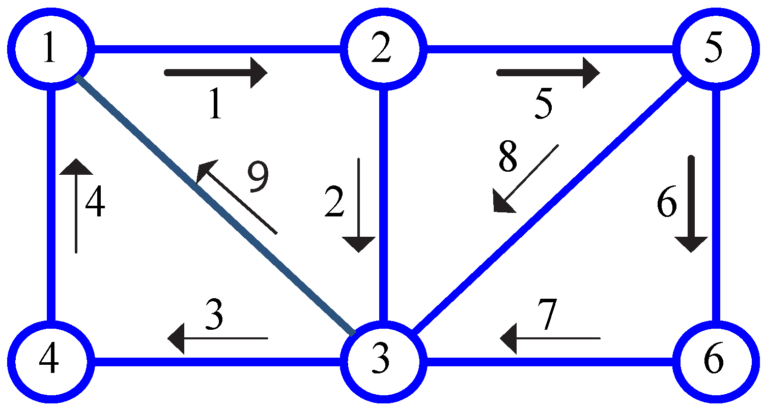
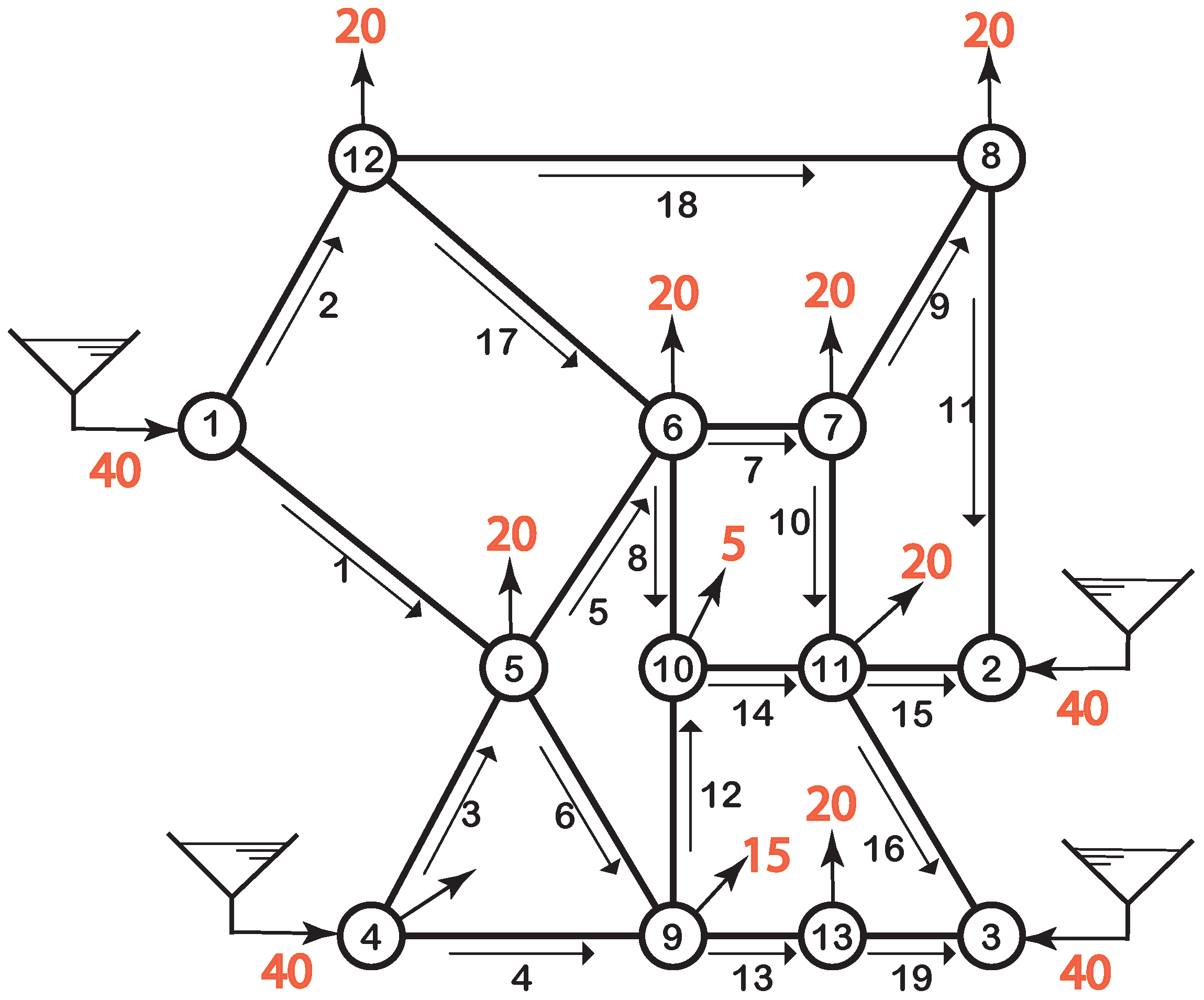
6.2. Application to Traffic Problems

Some applications to traffic problems are the following:

• The problem of optimizing the use of scanning resources for the estimation of route flows in traffic networks is dealt with in [40], where the authors analyze three problems: (a) how to minimize the number of cameras required for estimating a given subset of route flows, (b) finding the links to be scanned when n cameras are available, and (c) solving the same problems when errors are present. Finally, the Nguyen Dupuis, a small-sized and well-known network example, and the case of the city of Ciudad Real in Spain, are used to illustrate the methodology.
• The problem of observability of subsets $V_1$ of flows in terms of another subset $V_2$, when simultaneously different types of flows, links, nodes, routes, origin–destination (OD), plate scanned, etc., are considered, is discussed in [7]. There are two problems considered: (a) which flows in $V_1$ can be calculated in terms of the observed flows $V_2$, and (b) find the subset of flows $V_2$ that needs to be observed to obtain the flows in $V_1$. In addition, important theorems providing necessary and sufficient conditions for solving these two problems are given and they are illustrated by its application to three simple examples.
• The observability problem in traffic networks and the optimal location of scanning and counting devices, the treatment of plate scanning information, and the associated flow amount of information measured is dealt with. In addition, the problem of the optimal location of counters and plate scanning cameras is analyzed and illustrated with some illustrative and real examples.

6.3. Applications to Algebra Problems

In this subsection, the following algorithms and methods are given:

• A pivoting transformation or algorithm, to obtain the orthogonal linear subspace to a given linear subspace is presented in [6], by explaining the meaning of the tables resulting after introducing each generator of the initial linear subspace. In addition, this algorithm allows us to solve many problems of linear algebra avoiding some painful classical methods, such as calculating the rank of a matrix, its inverse and determinant, updating inverses and determinants of a matrix after changing rows or columns, identifying linearly dependent vectors, etc.
• The $\mathrm{\Gamma }$ algorithm, to obtain the dual cone of a given cone, is presented in some detail in [17]. This algorithm obtains, at the i-th step, the dual cone of the cone generated by the first generators of the initial cone. This algorithm is useful to solve a wide collection of algebra problems that can be solved if one uses the point of view of polarity, such as checking if a vector belongs to a cone, obtaining minimal representations of cones as the sum of a linear subspace and an acute cone, obtaining the cone intersection of two given cones, etc.
  Finally, the proposed methods and applications are illustrated with some examples.
• An interesting method that implies systems of linear equations subject to data with rounding errors is presented in [41], where, due to the errors, the linear system becomes incompatible. Thus, instead of solving the system, a least squares problem is solved, leading to another linear system. The methods mentioned in the present paper suggest alternative solutions to the problem.
• The problem of systems of linear equations when the less than or equal to, equal to or greater than, or equal to relations can be selected is solved in [20]. The proposed algorithm provides the necessary information to solve this problem, where the operators in each linear relation are chosen as wished. In addition, the algorithm permits obtaining the dual cone of the cone defined by any subset of constraints. Some examples illustrate the methodology.

7. Conclusions

The main conclusions that can be derived from this paper are:

• There exist a wide collection of methods and algorithms to deal with the problem of solving systems of linear inequalities and related problems, but they appear in some areas of mathematical specialities which are far from other applied areas in which these systems appear in a natural way.
• This causes a general state of ignorance about the possibilities of using these methods and algorithms to solve real and important problems in which they play an important role.
• People in general have a great degree of ignorance about the algebraic structures of polyhedra as the sum of a linear subspace plus an acute cone plus a polytope. In particular they ignore that for bounded problems this solution degenerates to a polytope, which is, with difference, the most frequent in real applications.
• The existing software able to solve systems of linear inequalities is not easily available, so that in practice this software is not commonly used in spite of its close relation with the problems mentioned. In addition, the software should be free to use.
• There is a need for publications describing the multiple applications of systems of linear inequalities. The actual lack of available examples and their poor diffusion is the cause of the slow rate of important advances in science and engineering.

References

1. Swart, G. Finding the convex hull facet by facet. J. Algorithms 1985, 6, 17–48. [Google Scholar] [CrossRef]
2. Avis, D.; Fukuda, K. A pivoting algorithm for convex hulls and vertex enumeration of arrangements and polyhedra. Discret. Comput. Geom. 1992, 8, 295–313. [Google Scholar] [CrossRef] [Green Version]
3. Ziegler, G.M. Lectures on Polytopes; Springer Science & Business Media: Berlin/Heidelberg, Germany, 2012; Volume 152. [Google Scholar]
4. Dyer, M.E. The Complexity of Vertex Enumeration Methods. Math. Oper. Res. 1983, 8, 381–402. [Google Scholar] [CrossRef]
5. Pang, L.P.; Spedicato, E.; Xia, Z.Q.; Wang, W. A method for solving the system of linear equations and linear inequalities. Math. Comput. Model. 2007, 46, 823–836. [Google Scholar] [CrossRef]
6. Castillo, E.; Cobo, A.; Jubete, F.; Pruneda, R.E.; Castillo, C. An Orthogonally Based Pivoting Transformation of Matrices and Some Applications. SIAM J. Matrix Anal. Appl. 2001, 22, 666–681. [Google Scholar] [CrossRef]
7. Castillo, E.; Gallego, I.; Sánchez-Cambronero, S.; Rivas, A. Matrix Tools for General Observability Analysis in Traffic Networks. IEEE Trans. Intell. Transp. Syst. 2010, 11, 799–813. [Google Scholar] [CrossRef]
8. Press, W.H.; Teukolsky, S.A.; Vetterling, W.T.; Flannery, B.P. Book Review: Numerical recipes: The art of scientific computing. by W. H. Press, B. P. Flannery, S. A. Teukolsky and W. T. Vetterling, Cambridge University Press, 1986, pp. xx + 818, price £25.00. J. Mol. Struct. 1987, 161, 349. [Google Scholar] [CrossRef]
9. Spedicato, E.; Bodon, E.; Del Popolo, A.; Xia, Z. ABS Algorithms for Linear Systems and Optimization. arXiv 2001, arXiv:math/0105056. [Google Scholar]
10. Abaffy, J.; Broyden, C.; Spedicato, E. A class of direct methods for linear systems. Numer. Math. 1984, 45, 361–376. [Google Scholar] [CrossRef]
11. Abaffy, J.; Spedicato, E. ABS Projection Algorithms: Mathematical Techniques for Linear and Nonlinear Equations; Prentice-Hall, Inc.: Hoboken, NJ, USA, 1989. [Google Scholar]
12. Nicolai, S.; Spedicato, E. A bibliography of the ABS methods. Optim. Methods Softw. 1997, 8, 171–183. [Google Scholar] [CrossRef]
13. Spedicato, E.; Bodon, E.; del Popolo, A.; Xia, Z. ABS algorithms for linear systems and optimization: A review and a bibliography. Cent. Eur. J. Oper. Res. 1999. [Google Scholar]
14. Spedicato, E.; Bodon, E.; Xia, Z.; Mahdavi-Amiri, N. ABS methods for continuous and integer linear equations and optimization. Cent. Eur. J. Oper. Res. 2010, 18, 73–95. [Google Scholar]
15. Demmel, J.W. Applied Numerical Linear Algebra; Society for Industrial and Applied Mathematics: Philadelphia, PA, USA, 1997. [Google Scholar] [CrossRef]
16. Higham, N.J. Accuracy and Stability of Numerical Algorithms, 2nd ed.; Society for Industrial and Applied Mathematics: Philadelphia, PA, USA, 2002. [Google Scholar] [CrossRef] [Green Version]
17. Castillo, E.; Jubete, F. The Γ-algorithm and some applications. Int. J. Math. Educ. Sci. Technol. 2004, 35, 369–389. [Google Scholar] [CrossRef]
18. Castillo, E.; Cobo, A.; Jubete, F.; Pruneda, R.E. Orthogonal Sets and Polar Methods in Linear Algebra: Applications to Matrix Calculations, Systems of Equations, Inequalities, and Linear Programming; Wiley Interscience. John Wiley and Sons: Hoboken, NJ, USA, 1999. [Google Scholar]
19. Pillers Dobler, C. A Matrix Approach to Finding a Set of Generators and Finding the Polar (Dual) of a Class of Polyhedral Cones. SIAM J. Matrix Analuysis Appl. 1994, 15, 796–803. [Google Scholar] [CrossRef]
20. Castillo, E.; Jubete, F.; Pruneda, R.; Solares, C. Obtaining simultaneous solutions of linear subsystems of inequalities and duals. Linear Algebra Its Appl. 2002, 346, 131–154. [Google Scholar] [CrossRef] [Green Version]
21. Contesse, L. A general algorithm for determining all essential solutions and inequalities for any convex polyhedron. Ann. Oper. Res. 1994, 50, 187–218. [Google Scholar] [CrossRef]
22. McMullen, P.G.M. Ziegler Lectures on polytopes (Graduate Texts in Mathematics, Vol. 152, Springer-Verlag, Berlin-Heidelberg-New York-London-Paris-Tokyo-Hong Kong 1995), ix 370 pp., softcover: 3 540 94365 X, £21, hardcover: 3 540 94329 3, £47. Proc. Edinb. Math. Soc. 1996, 39, 189–190. [Google Scholar] [CrossRef] [Green Version]
23. Matheiss, T.H.; Rubin, D.S. A Survey and Comparison of Methods for Finding All Vertices of Convex Polyhedral Sets. Math. Oper. Res. 1980, 5, 167–185. [Google Scholar] [CrossRef]
24. Dyer, M.; Proll, L. An improved vertex enumeration algorithm. Eur. J. Oper. Res. 1982, 9, 359–368. [Google Scholar] [CrossRef]
25. Motzkin, T.S.; Raiffa, H.; Thompson, G.L.; Thrall, R.M. The double description method. Contrib. Theory Games 1953, 2, 51–73. [Google Scholar]
26. Fukuda, K.; Prodon, A. Double description method revisited. In Franco-Japanese and Franco-Chinese Conference on Combinatorics and Computer Science; Deza, M., Euler, R., Manoussakis, I., Eds.; Springer: Berlin/Heidelberg, Germany, 1996; pp. 91–111. [Google Scholar]
27. Esmaeili, H.; Mahdavi-Amiri, N. Solving some linear inequality systems and LP problems in real and integer spaces via the ABS algorithm. QDMSIA13 2000. [Google Scholar]
28. Zhao, J. A class of direct methods for solving linear inequalities. J. Numer. Math. Chin. Univ. 1989, 3, 231–238. [Google Scholar]
29. Shi, G. An ABS algorithm for generating nonnegative solutions of linear systems. In Proceedings of the First International Conference on ABS Algorithms, Luoyang, China, 2–6 September 1991; pp. 54–57. [Google Scholar]
30. Gill, P.E.; Golub, G.H.; Murray, W.; Saunders, M.A. Methods for modifying matrix factorizations. Math. Comp. 1974, 28, 505–535. [Google Scholar] [CrossRef]
31. Zhang, L. A method for finding a feasible point of inequalities. In Proceedings of the First International Conference on ABS Algorithms, Luoyang, China, 2–6 September 1991; pp. 131–137. [Google Scholar]
32. Zhang, L. An algorithm for the least Euclidean norm solution of a linear system of inequalities via the Huang ABS algorithm and the Goldfarb–Idnani strategy. Rep. DMSIA 1995, 95. [Google Scholar]
33. Xia, Y.; Wang, J.; Hung, D.L. Recurrent neural networks for solving linear inequalities and equations. IEEE Trans. Circuits Syst. I Fundam. Theory Appl. 1999, 46, 452–462. [Google Scholar]
34. Xu, F.; Li, Z.; Nie, Z.; Shao, H.; Guo, D. Zeroing Neural Network for Solving Time-Varying Linear Equation and Inequality Systems. IEEE Trans. Neural Netw. Learn. Syst. 2019, 30, 2346–2357. [Google Scholar] [CrossRef] [PubMed]
35. Chvatal, V. Linear Programming; Macmillan: New York, NY, USA, 1983. [Google Scholar]
36. Padberg, M. Linear Programming and Extensions; Springer: Berlin, Germany, 1995. [Google Scholar]
37. Scrucca, L. Entropy-Based Anomaly Detection for Gaussian Mixture Modeling. Algorithms 2023, 16, 195. [Google Scholar] [CrossRef]
38. La Grassa, R.; Gallo, I.; Vetro, C.; Landro, N. Learning to Navigate in the Gaussian Mixture Surface. In International Conference on Computer Analysis of Images and Patterns; Tsapatsoulis, N., Panayides, A., Theocharides, T., Lanitis, A., Pattichis, C., Vento, M., Eds.; Springer International Publishing: Cham, Switzerland, 2021; pp. 414–423. [Google Scholar]
39. Karras, C.; Karras, A.; Giotopoulos, K.C.; Avlonitis, M.; Sioutas, S. Consensus Big Data Clustering for Bayesian Mixture Models. Algorithms 2023, 16, 245. [Google Scholar] [CrossRef]
40. Castillo, E.; Gallego, I.; Menéndez, J.M.; Rivas, A. Optimal Use of Plate-Scanning Resources for Route Flow Estimation in Traffic Networks. IEEE Trans. Intell. Transp. Syst. 2010, 11, 380–391. [Google Scholar] [CrossRef]
41. Lukyanenko, D. Parallel Algorithm for Solving Overdetermined Systems of Linear Equations, Taking into Account Round-Off Errors. Algorithms 2023, 16, 242. [Google Scholar] [CrossRef]
Figure 1. Simple example network.
Algorithms 16 00356 g001
Figure 2. The water supply network in example 1, showing the water flows x 1 to x 19 , the input flows q 1 to q 4 , and the output flows q 5 to q 13 .
Algorithms 16 00356 g002