Article

Lipschitz Continuity Results for a Class of Parametric Variational Inequalities and Applications to Network Games

by
Mauro Passacantando
1 and
Fabio Raciti
2,*
1
Department of Business and Law, University of Milan-Bicocca, Via degli Arcimboldi 8, 20126 Milan, Italy
2
Department of Mathematics and Computer Science, University of Catania, Viale A. Doria 6, 95125 Catania, Italy
*
Author to whom correspondence should be addressed.
Algorithms 2023, 16(10), 458; https://doi.org/10.3390/a16100458
Submission received: 31 August 2023 / Revised: 21 September 2023 / Accepted: 25 September 2023 / Published: 26 September 2023
(This article belongs to the Special Issue Recent Advances in Nonsmooth Optimization and Analysis)

Abstract

:
We consider a class of finite-dimensional variational inequalities where both the operator and the constraint set can depend on a parameter. Under suitable assumptions, we provide new estimates for the Lipschitz constant of the solution, which considerably improve previous ones. We then consider the problem of computing the mean value of the solution with respect to the parameter and, to this end, adapt an algorithm devised to approximate a Lipschitz function whose analytic expression is unknown, but can be evaluated in arbitrarily chosen sample points. Finally, we apply our results to a class of Nash equilibrium problems, and generalized Nash equilibrium problems on networks.

1. Introduction

In many optimization or variational inequality (VI) problems, some data can depend on parameters, and it is important to analyze the regularity of the solution with respect to those parameters. For a detailed account of some classical results on the topic of parametric optimization, the reader can refer to [1]. The investigation of the Lipschitz behavior of solutions to convex minimization problems, from the point of view of set valued analysis, has also been carried out in the influential paper [2], and recently extended to abstract quasi-equilibrium problems in [3]. On a more applied context, in the case of linear programming, sharp Lipschitz constants for feasible and optimal solutions of some perturbed linear programs were derived in [4,5]. Another influential paper focusing on the estimate of Lipschitz constants for the solutions of a perturbed system of equalities and inequalities is [6], while in [7], the estimate of the Lipschitz constant is connected with of the role played by the norm of the inverse of a non-singular matrix in bounding the perturbation of the solution of a system of equations in terms of a right-hand side perturbation. The topic of parametric sensitivity analysis for variational inequalities has been developed by many authors in recent decades, and the excellent monograph [8] contains many related results. Let us notice, however, that while the number of papers dealing with local parametric differentiability for variational inequalities is very large, the investigation of parametric variational inequalities under the mere Lipschitz assumptions on data have received less attention, in particular with respect to the problem of estimating the global Lipschitz constant of the solution.
The local Lipschitz continuity of the solution of a variational inequality with parametric constraint set was investigated in [9], while more recently, the authors [10] derived an estimate of the global Lipschitz constant of the unique solution of a parametrized variational inequality, by making an extensive use of Lagrange multipliers techniques. Specifically, the Lagrange multiplier computations were used to derive the contribution of the parametric variation in the constraint set to the corresponding variation in the solution of the variational inequality. Interestingly enough, similar results were obtained in [11] with purely geometric methods. In [12], the authors improved the above-mentioned estimate but realized that, due to the complexity of the problem, their estimates were also far from being optimal.
In this paper, we derive new estimates for the Lipschitz constant of the solution of a parametric variational inequality, which considerably improve the previous ones. We then combine our results with a variant of the algorithm proposed in [13,14] to provide an approximation, on a given interval, of a univariate Lipschitz function whose analytic expression is unknown, but can be computed in arbitrarily chosen sample points (such a function is often called a black box-function). It turns out that the same algorithm also provides an approximation of the integral of the black-box function on the interval under consideration. Thus, we can use our estimate of the Lipschitz constant of the solution, to approximate its mean value on a given interval. Our results are then applied to investigate a class of Nash and generalized Nash equilibrium problems on networks.
The specific class of Nash equilibrium problems known as Network Games (or games played on networks) was investigated for the first time in the paper by Ballester et al. [15]. Players are modeled as nodes of a graph, and the social or economic relationship between any two players is represented by a link connecting the two corresponding nodes. Two players connected with a link are called neighbors. Considering linear-quadratic utility functions, the authors were able to express the unique Nash equilibrium as a series expansion involving the powers of the adjacency matrix of the graph, thus showing that, although players only interact with their neighbors, the equilibrium also depends on indirect contacts (i.e., neighbors of neighbors, neighbors of neighbors of neighbors, and so on). A wealth of social and economic processes may be modeled using the theory of Network Games; see, for instance, the papers [16,17,18,19], the survey [20] and the monograph [21]. The solution methods used in all the above-mentioned references combine the best response approach with some results of Graph Theory (see, e.g., [22]). It is worth noticing that although the connection between variational inequalities and Nash equilibrium problems was proven about forty years ago [23], very few papers have dealt with the variational inequality approach to Network Games and, in this regard, the interested reader can find a detailed investigation in [24]. Furthermore, the case of generalized network Nash equilibrium problems with shared constraints has not yet been investigated within the above-mentioned framework, with the only exception of the paper [25].
The paper is organized as follows. In Section 2, we provide estimates of the Lipschitz constant of the solution of our parametric VI in a general case, as well as in four different cases where the dependence on the parameter is more specific. In Section 3, we describe the algorithm used to approximate the solution components and their mean values. Section 4 is devoted to the application of our results to a class of Network Games, and is structured in three subsections. Specifically, in Section 4.1 we provide the basic concepts on Network Games, in Section 4.2 we describe the quadratic reference model of a network Nash equilibrium problem, while in Section 4.3 we first recall the definition of generalized Nash equilibrium problem with shared constraints, and the concept of variational solution, and then consider the quadratic reference model in this new setting. In Section 5, we apply our estimates and algorithm to some parametric network games. We then summarize our work and outline some future research perspectives in a small conclusion section. The paper ends with Appendix A, where we derive some exact results that can be obtained in the special case where the Lipschitz constant of the operator of the variational inequality equals its strong monotonicity constant.

2. Problem Formulation and Lipschitz Constant Estimates

Let F : [ 0 , T ] × R n R n and, for each t [ 0 , T ] , K ( t ) be a nonempty, closed and convex subset of R n . We denote with · , · the scalar product in R n . The variational inequality on R n , with parameter t [ 0 , T ] , is the following problem: for each t [ 0 , T ] , find x ( t ) K ( t ) such that:
F ( t , x ( t ) ) , y x ( t ) 0 , y K ( t ) .
In the case where, for each t [ 0 , T ] the solution of (1) is unique, we will prove, assuming the Lipschitz continuity of F and of the parametric functions describing K ( t ) , the Lipschitz continuity of the solution map t x ( t ) and derive an a priori estimate of its Lipschitz constant Λ . Specifically, we estimate Λ in the general case where the variables t and x cannot be separated, as well as in the separable case where F ( t , x ) = G ( x ) + H ( t ) . Moreover, in the special circumstance where K ( t ) = K , for any t [ 0 , T ] , two simplified formulas are derived. We then focus on computing approximations for the mean value of the components x j : [ 0 , T ] R , j = 1 , n :
1 T 0 T x j ( t ) d t .
We recall here some useful monotonicity properties.
Definition 1. 
A map F : R n R n is monotone on a set A R n if and only if
F ( x ) F ( y ) , x y 0 , x , y A .
If the equality holds only when x = y , F is said to be strictly monotone.
A stronger type of monotonicity is given by the following definition.
Definition 2. 
F : R n R n is α-strongly monotone on A if and only if α > 0 :
F ( x ) F ( y ) , x y α x y 2 , x , y A .
The concepts of strict and strong monotonicity coincide for linear operators and they are equivalent to the positive definiteness of the corresponding matrix. When F also depends on a parameter, the following property is useful.
Definition 3. 
F : [ 0 , T ] × R n R n is uniformly α-strongly monotone on A if and only if α > 0 :
F ( t , x ) F ( t , y ) , x y α x y 2 x , y A , t [ 0 , T ] .
Sufficient conditions for the existence and uniqueness of the solution of a variational inequality problem can be found in [8]. We mention here the following classical theorem which, in the parametric case, has to be applied for each t [ 0 , T ] .
Theorem 1. 
Let K R n be a closed and convex set and F : R n R n continuous on K. If K is bounded, then the variational inequality problem V I ( F , K ) admits at least one solution. If K is unbounded, then the existence of a solution is guaranteed by the following coercivity condition:
lim x + F ( x ) F ( x 0 ) , x x 0 x x 0 = + ,
for x K and some x 0 K . Furthermore, if F is α-strongly monotone on K, then the solution exists and is unique.
Let us now prove two theorems, along with three corresponding corollaries, which constitute the main contribution of the paper. Such results, at different levels of generality, ensure that the unique solution of (1) is Lipschitz continuous, and also provide an estimate of the Lipschitz constant of the solution.
Theorem 2 (General case). 
Assume that F : [ 0 , T ] × R n R n is uniformly α-strongly monotone on R n and F is Lipschitz continuous on [ 0 , T ] × R n with constant L, i.e.,
F ( t 1 , x 1 ) F ( t 2 , x 2 ) L ( | t 1 t 2 | + x 1 x 2 ) , x 1 , x 2 R n , t 1 , t 2 [ 0 , T ] .
Moreover, we assume that K ( t ) is a closed and convex set for any t [ 0 , T ] , and there exists M 0 such that
p K ( t 1 ) ( x ) p K ( t 2 ) ( x ) M | t 1 t 2 | , x R n , t 1 , t 2 [ 0 , T ] ,
where p K ( t ) ( x ) denotes the projection of x on the closed convex set K ( t ) .
Then, for any t [ 0 , T ] , there exists a unique solution x ( t ) of the V I ( F , K ( t ) ) and x ( t ) is Lipschitz continuous on [ 0 , T ] , with an estimated constant equal to
Λ 1 = inf z 0 , 2 α ˜ M 1 s + z ( 1 + z ) s ( 1 s ) , if α ˜ < 1 , M + 2 2 M + 1 , if α ˜ = 1 ,
where α ˜ = α / L and s = z 2 2 α ˜ z + 1 .
Proof. 
The existence and uniqueness of the solution x ( t ) follows from Theorem 1. Given t 1 , t 2 [ 0 , T ] , we denote x 1 : = x ( t 1 ) and x 2 : = x ( t 2 ) . We know that
x 1 = p K ( t 1 ) ( x 1 λ F ( t 1 , x 1 ) ) , x 2 = p K ( t 2 ) ( x 2 λ F ( t 2 , x 2 ) ) ,
hold for any λ > 0 , due to the characterization of the projection onto a closed convex set and the Brower fixed point theorem (see, e.g., [8]). Hence, we obtain the following estimate:
x 2 x 1 = p K ( t 2 ) ( x 2 λ F ( t 2 , x 2 ) ) p K ( t 1 ) ( x 1 λ F ( t 1 , x 1 ) ) p K ( t 2 ) ( x 2 λ F ( t 2 , x 2 ) ) p K ( t 1 ) ( x 2 λ F ( t 2 , x 2 ) ) + p K ( t 1 ) ( x 2 λ F ( t 2 , x 2 ) ) p K ( t 1 ) ( x 1 λ F ( t 1 , x 1 ) ) M | t 1 t 2 | + ( x 2 λ F ( t 2 , x 2 ) ) ( x 1 λ F ( t 1 , x 1 ) ) ,
where the second inequality follows from assumption (3) and the non-expansiveness of the projection map. Moreover, we have
( x 2 λ F ( t 2 , x 2 ) ) ( x 1 λ F ( t 1 , x 1 ) ) 2 = x 2 x 1 2 + λ 2 F ( t 2 , x 2 ) F ( t 1 , x 1 ) 2 2 λ x 2 x 1 , F ( t 2 , x 2 ) F ( t 1 , x 1 ) x 2 x 1 2 + λ 2 L 2 ( x 2 x 1 + | t 2 t 1 | ) 2 2 λ x 2 x 1 , F ( t 2 , x 2 ) F ( t 1 , x 1 ) = x 2 x 1 2 + λ 2 L 2 ( x 2 x 1 + | t 2 t 1 | ) 2 2 λ x 2 x 1 , F ( t 2 , x 2 ) F ( t 2 , x 1 ) 2 λ x 2 x 1 , F ( t 2 , x 1 ) F ( t 1 , x 1 ) x 2 x 1 2 + λ 2 L 2 ( x 2 x 1 + | t 2 t 1 | ) 2 2 λ α x 2 x 1 2 + 2 λ x 2 x 1 F ( t 2 , x 1 ) F ( t 1 , x 1 ) = x 2 x 1 2 + λ 2 L 2 ( x 2 x 1 + | t 2 t 1 | ) 2 2 λ α x 2 x 1 2 + 2 λ L x 2 x 1 | t 2 t 1 | = ( 1 + λ 2 L 2 2 λ α ) x 2 x 1 2 + λ 2 L 2 | t 2 t 1 | 2 + 2 λ L ( 1 + λ L ) x 2 x 1 | t 2 t 1 | .
It is well-known that α L , since the assumptions guarantee that the following inequalities
α x y 2 F ( t , x ) F ( t , y ) , x y F ( t , x ) F ( t , y ) x y L x y 2
hold for any x , y R n and t [ 0 , T ] . Thus, we obtain
1 + λ 2 L 2 2 λ α 1 + λ 2 L 2 2 λ L = ( 1 λ L ) 2 0 ,
hence s : = 1 + λ 2 L 2 2 λ α is well defined. Notice that if α < L , then s > 0 for any λ > 0 , while if α = L then s > 0 for any λ ( 0 , 1 / L ) ( 1 / L , + ) . Moreover, we have
1 + λ L = 1 + λ 2 L 2 + 2 λ L > 1 + λ 2 L 2 2 λ α = s ,
thus, if s > 0 , we have
λ 2 L 2 | t 2 t 1 | 2 λ L 1 + λ L s | t 2 t 1 | 2 .
It follows from (5) and (6) that
( x 2 λ F ( t 2 , x 2 ) ) ( x 1 λ F ( t 1 , x 1 ) ) 2 ( s x 2 x 1 ) 2 + λ L 1 + λ L s | t 2 t 1 | 2 + 2 λ L ( 1 + λ L ) x 2 x 1 | t 2 t 1 | = s x 2 x 1 + λ L 1 + λ L s | t 2 t 1 | 2 ,
hence
( x 2 λ F ( t 2 , x 2 ) ) ( x 1 λ F ( t 1 , x 1 ) ) s x 2 x 1 + λ L 1 + λ L s | t 2 t 1 | .
It follows from (4) and (7) that
( 1 s ) x 2 x 1 M + λ L ( 1 + λ L ) s | t 2 t 1 | .
Notice that 1 s > 0 if and only if λ ( 0 , 2 α / L 2 ) . Therefore, in the case α < L , we obtain
x 2 x 1 M 1 s + λ L ( 1 + λ L ) s ( 1 s ) | t 2 t 1 | , λ 0 , 2 α L 2 ,
while in the case α = L , we obtain
x 2 x 1 M 1 s + λ L ( 1 + λ L ) s ( 1 s ) | t 2 t 1 | , λ 0 , 1 L 1 L , 2 L .
If we set z = λ L and α ˜ = α / L , then we can write s = z 2 2 α ˜ z + 1 and the estimate (8), which, in case α ˜ < 1 , reads as
x 2 x 1 inf z ( 0 , 2 α ˜ ) M 1 s + z ( 1 + z ) s ( 1 s ) | t 2 t 1 | .
In case α ˜ = 1 , we have s = | z 1 | , and the estimate (9) reads as
x 2 x 1 inf z ( 0 , 1 ) ( 1 , 2 ) f ( z ) | t 2 t 1 | ,
where
f ( z ) = M 1 | z 1 | + z ( 1 + z ) | z 1 | ( 1 | z 1 | ) = M z + 1 + z 1 z if z ( 0 , 1 ) , M 2 z + z ( 1 + z ) ( z 1 ) ( 2 z ) if z ( 1 , 2 ) .
An analytical study of the function f (see Appendix A.1) provides
inf z ( 0 , 1 ) f ( z ) = M + 2 2 M + 1 ,
and
inf z ( 1 , 2 ) f ( z ) = M 2 + 7 M + 8 + 2 2 M + 12 M + 8 2 2 M + 12 .
Moreover, it is easy to check that the following inequality
inf z ( 1 , 2 ) f ( z ) inf z ( 0 , 1 ) f ( z )
holds for any M 0 . Therefore, we obtain
inf z ( 0 , 1 ) ( 1 , 2 ) f ( z ) = inf z ( 0 , 1 ) f ( z ) = M + 2 2 M + 1 ,
thus the thesis follows. □
Corollary 1 (General operator and constant feasible region). 
Assume that F satisfies the same assumptions of Theorem 2 and the feasible region K does not depend on t. Then, the solution x ( t ) of the VI( F , K ) is Lipschitz continuous on [ 0 , T ] with estimated constant equal to Λ 1 = L / α .
Proof. 
Since K does not depend on t, inequality (3) holds with M = 0 . Hence, Theorem 2 guarantees that x ( t ) is Lipschitz continuous on [ 0 , T ] with a constant equal to
inf z 0 , 2 α ˜ z ( 1 + z ) s ( 1 s ) , if α ˜ < 1 , 1 , if α ˜ = 1 ,
where α ˜ = α / L and s = z 2 2 α ˜ z + 1 . It is sufficient to prove that if α ˜ < 1 , then
inf z 0 , 2 α ˜ z ( 1 + z ) s ( 1 s ) = 1 α ˜ .
Since α ˜ > 0 , we have
( 1 + α ˜ ) z 2 2 α ˜ z + 1 + α ˜ > 0 , z R ,
thus
( 1 + α ˜ ) z 2 ( 1 + α ˜ ) z 2 2 α ˜ z + 1 + α ˜ > 0 , z > 0 ,
On the other hand, we have
( 1 + α ˜ ) z 2 ( 1 + α ˜ ) z 2 2 α ˜ z + 1 + α ˜ = ( 1 + α ˜ ) 2 z 4 2 α ˜ ( 1 + α ˜ ) z 3 + ( 1 + α ˜ ) 2 z 2 = ( 1 + α ˜ ) 2 z 4 + α ˜ 2 z 2 + 1 2 α ˜ ( 1 + α ˜ ) z 3 + 2 ( 1 + α ˜ ) z 2 2 α ˜ z z 2 + 2 α ˜ z 1 = [ ( 1 + α ˜ ) z 2 α ˜ z + 1 ] 2 z 2 + 2 α ˜ z 1 = [ ( 1 + α ˜ ) z 2 α ˜ z + 1 ] 2 s 2 ,
hence
[ ( 1 + α ˜ ) z 2 α ˜ z + 1 ] 2 > s 2 , z > 0 .
Since s > 0 and ( 1 + α ˜ ) z 2 α ˜ z + 1 > 0 hold for any z > 0 , we obtain
( 1 + α ˜ ) z 2 α ˜ z + 1 > s , z > 0 .
The latter inequality is equivalent to
α ˜ z ( 1 + z ) > s z 2 + 2 α ˜ z 1 = s ( 1 s ) , z > 0 .
Since s > 0 and 1 s > 0 hold for any z ( 0 , 2 α ˜ ) , we obtain
z ( 1 + z ) s ( 1 s ) > 1 α ˜ , z ( 0 , 2 α ˜ ) .
On the other hand, we have
lim z 0 z ( 1 + z ) s ( 1 s ) = lim z 0 z ( 1 + z ) ( 1 + s ) s ( 1 s 2 ) = lim z 0 z ( 1 + z ) ( 1 + s ) s z ( 2 α ˜ z ) = lim z 0 ( 1 + z ) ( 1 + s ) s ( 2 α ˜ z ) = 1 α ˜ .
Therefore, the proof is complete. □
Theorem 3 (Separable operator). 
Assume that F : [ 0 , T ] × R n R n is separable, i.e,
F ( t , x ) = G ( x ) + H ( t ) , t [ 0 , T ] , x R n ,
where G : R n R n is α-strongly monotone on R n and Lipschitz continuous on R n with constant L x , and H : [ 0 , T ] R n is Lipschitz continuous on R n with constant L t . Moreover, we assume that K ( t ) is a closed and convex set for any t [ 0 , T ] , and there exists M 0 , such that (3) holds.
Then, for any t [ 0 , T ] , there exists a unique solution x ( t ) of the V I ( F , K ( t ) ) , and x ( t ) is Lipschitz continuous on [ 0 , T ] with an estimated constant equal to
Λ 2 = inf z 0 , 2 α ^ M 1 s ^ + L ^ z ( 1 + z ) s ^ ( 1 s ^ ) , if α ^ < 1 , M + 2 2 M L ^ + L ^ , if α ^ = 1 ,
where α ^ = α / L x , L ^ = L t / L x and s ^ = z 2 2 α ^ z + 1 .
Proof. 
The existence and uniqueness of the solution x ( t ) follows from Theorem 1. Given t 1 , t 2 [ 0 , T ] , we denote x 1 : = x ( t 1 ) and x 2 : = x ( t 2 ) . For any λ > 0 , we have the following estimate:
x 2 x 1 = p K ( t 2 ) ( x 2 λ F ( t 2 , x 2 ) ) p K ( t 1 ) ( x 1 λ F ( t 1 , x 1 ) ) p K ( t 2 ) ( x 2 λ F ( t 2 , x 2 ) ) p K ( t 1 ) ( x 2 λ F ( t 2 , x 2 ) ) + p K ( t 1 ) ( x 2 λ F ( t 2 , x 2 ) ) p K ( t 1 ) ( x 1 λ F ( t 1 , x 1 ) ) M | t 1 t 2 | + ( x 2 λ F ( t 2 , x 2 ) ) ( x 1 λ F ( t 1 , x 1 ) ) .
Moreover, we have
( x 2 λ F ( t 2 , x 2 ) ) ( x 1 λ F ( t 1 , x 1 ) ) 2 = x 2 x 1 2 + λ 2 F ( t 2 , x 2 ) F ( t 1 , x 1 ) 2 2 λ x 2 x 1 , F ( t 2 , x 2 ) F ( t 1 , x 1 ) = x 2 x 1 2 + λ 2 G ( x 2 ) G ( x 1 ) + H ( t 2 ) H ( t 1 ) 2 2 λ x 2 x 1 , G ( x 2 ) G ( x 1 2 λ x 2 x 1 , H ( t 2 ) H ( t 1 ) x 2 x 1 2 + λ 2 ( L x x 2 x 1 + L t | t 2 t 1 | ) 2 2 λ x 2 x 1 , G ( x 2 ) G ( x 1 2 λ x 2 x 1 , H ( t 2 ) H ( t 1 ) x 2 x 1 2 + λ 2 ( L x x 2 x 1 + L t | t 2 t 1 | ) 2 2 λ α x 2 x 1 2 + 2 λ x 2 x 1 H ( t 2 ) H ( t 1 ) x 2 x 1 2 + λ 2 ( L x x 2 x 1 + L t | t 2 t 1 | ) 2 2 λ α x 2 x 1 2 + 2 λ L t x 2 x 1 | t 2 t 1 | = ( 1 + λ 2 L x 2 2 λ α ) x 2 x 1 2 + λ 2 L t 2 | t 2 t 1 | 2 + 2 λ L t ( 1 + λ L x ) x 2 x 1 | t 2 t 1 | .
Since α L x , we have
1 + λ 2 L x 2 2 λ α 1 + λ 2 L x 2 2 λ L x = ( 1 λ L x ) 2 0 ,
hence s ^ : = 1 + λ 2 L x 2 2 λ α is well defined. Notice that if α < L x , then s > 0 for any λ > 0 , while if α = L x , then s > 0 for any λ ( 0 , 1 / L x ) ( 1 / L x , + ) . Moreover, we have
1 + λ L x = 1 + λ 2 L x 2 + 2 λ L x > 1 + λ 2 L x 2 2 λ α = s ^ ,
thus, if s ^ > 0 , we have
λ 2 L t 2 | t 2 t 1 | 2 λ L t 1 + λ L x s ^ | t 2 t 1 | 2 .
It follows from (11) and (12) that
( x 2 λ F ( t 2 , x 2 ) ) ( x 1 λ F ( t 1 , x 1 ) ) 2 ( s ^ x 2 x 1 ) 2 + λ L t 1 + λ L x s ^ | t 2 t 1 | 2 + 2 λ L t ( 1 + λ L x ) x 2 x 1 | t 2 t 1 | = s ^ x 2 x 1 + λ L t 1 + λ L x s ^ | t 2 t 1 | 2 ,
hence
( x 2 λ F ( t 2 , x 2 ) ) ( x 1 λ F ( t 1 , x 1 ) ) s ^ x 2 x 1 + λ L t 1 + λ L x s ^ | t 2 t 1 | .
It follows from (10) and (13) that
( 1 s ^ ) x 2 x 1 M + λ L t ( 1 + λ L x ) s ^ | t 2 t 1 | .
Notice that 1 s ^ > 0 if and only if λ ( 0 , 2 α / L x 2 ) . Therefore, in the case α < L x , we obtain
x 2 x 1 M s ^ + λ L t ( 1 + λ L x ) s ^ ( 1 s ^ ) | t 2 t 1 | , λ 0 , 2 α L x 2 ,
while in the case α = L x , we obtain
x 2 x 1 M s ^ + λ L t ( 1 + λ L x ) s ^ ( 1 s ^ ) | t 2 t 1 | , λ 0 , 1 L x 1 L x , 2 L x .
If we set z = λ L x , α ^ = α / L x and L ^ = L t / L x , then we can write s ^ = z 2 2 α ^ z + 1 , and the estimate (14), in the case α ^ < 1 , reads as
x 2 x 1 inf z ( 0 , 2 α ^ ) M 1 s ^ + L ^ z ( 1 + z ) s ^ ( 1 s ^ ) | t 2 t 1 | .
In the case α ^ = 1 , we have s ^ = | z 1 | and the estimate (15) reads as
x 2 x 1 inf z ( 0 , 1 ) ( 1 , 2 ) f ( z ) | t 2 t 1 | ,
where
f ( z ) = M 1 | z 1 | + L ^ z ( 1 + z ) | z 1 | ( 1 | z 1 | ) = M z + L ^ ( 1 + z ) 1 z if z ( 0 , 1 ) , M 2 z + L ^ z ( 1 + z ) ( z 1 ) ( 2 z ) if z ( 1 , 2 ) .
An analytical study of the function f (see Appendix A.2) provides
inf z ( 0 , 1 ) f ( z ) = M + 2 2 M L ^ + L ^ ,
and
inf z ( 1 , 2 ) f ( z ) = M 2 + 7 M L ^ + 8 L ^ 2 + 2 L ^ 2 M L ^ + 12 L ^ 2 M + 8 L ^ 2 2 M L ^ + 12 L ^ 2 .
Moreover, it is easy to check that the following inequality
inf z ( 1 , 2 ) f ( z ) inf z ( 0 , 1 ) f ( z )
holds for any M 0 and L ^ > 0 . Therefore, we obtain
inf z ( 0 , 1 ) ( 1 , 2 ) f ( z ) = inf z ( 0 , 1 ) f ( z ) = M + 2 2 M L ^ + L ^ ,
thus the thesis follows. □
Corollary 2 (Separable operator and constant feasible region). 
Assume that F satisfies the assumptions of Theorem 3 and the feasible region K does not depend on t. Then, the solution x ( t ) of the VI( F , K ) is Lipschitz continuous on [ 0 , T ] with estimated constant equal to Λ 2 = L t / α .
Proof. 
Theorem 3 guarantees that x ( t ) is Lipschitz continuous on [ 0 , T ] with a constant equal to
inf z 0 , 2 α ^ L ^ z ( 1 + z ) s ^ ( 1 s ^ ) , if α ^ < 1 , L ^ = L t / α , if α ^ = 1 ,
where α ^ = α / L x , L ^ = L t / L x and s ^ = z 2 2 α ^ z + 1 . Moreover, similarly to the proof of Corollary 1, where α ˜ is replaced by α ^ , it can be proved that if α ^ < 1 , then
inf z 0 , 2 α ^ L ^ z ( 1 + z ) s ^ ( 1 s ^ ) = L ^ α ^ = L t α .
In the special case where F does not depend on t, we obtain the same estimate proved in [12].
Corollary 3 (Constant operator). 
Assume that F and K satisfy the assumptions of Theorem 3 and F does not depend on t, i.e., H ( t ) 0 . Then, the solution x ( t ) of the VI( F , K ) is Lipschitz continuous on [ 0 , T ] with estimated constant equal to
Λ 2 = M 1 1 α L 2 .
Proof. 
If H ( t ) 0 , then L t = 0 , and Theorem 3 guarantees that x ( t ) is Lipschitz continuous on [ 0 , T ] with a constant equal to
inf z 0 , 2 α ^ M 1 s ^ , if α ^ < 1 , M , if α ^ = 1 ,
where α ^ = α / L x = α / L and s ^ = z 2 2 α ^ z + 1 .
Moreover, it is easy to check that
inf z 0 , 2 α ^ M 1 s ^ = M 1 1 α ^ 2 = M 1 1 α L 2 ,
thus the thesis follows. □
Table 1 summarizes the estimate of the Lipschitz constant of x ( t ) depending on the features of the map F and the feasible set K.
Theorems 2 and 3, along with Corollaries 1, 2 and 3, do not provide the solution x ( t ) of the parametric VI in closed form, but guarantee that it is a Lipschitz continuous function of the parameter t and provide an estimate of the corresponding constant. The knowledge of the Lipschitz constant is a key tool to provide lower and upper approximations of both the solution x ( t ) and its mean value on [ 0 , T ] , as the algorithm described in the next section shows.

3. Approximation Algorithm

Let x j : [ 0 , T ] R be any component of the solution vector x of (1); assume that x j is a Lipschitz continuous function and Λ is an estimate of its Lipschitz constant, i.e.,
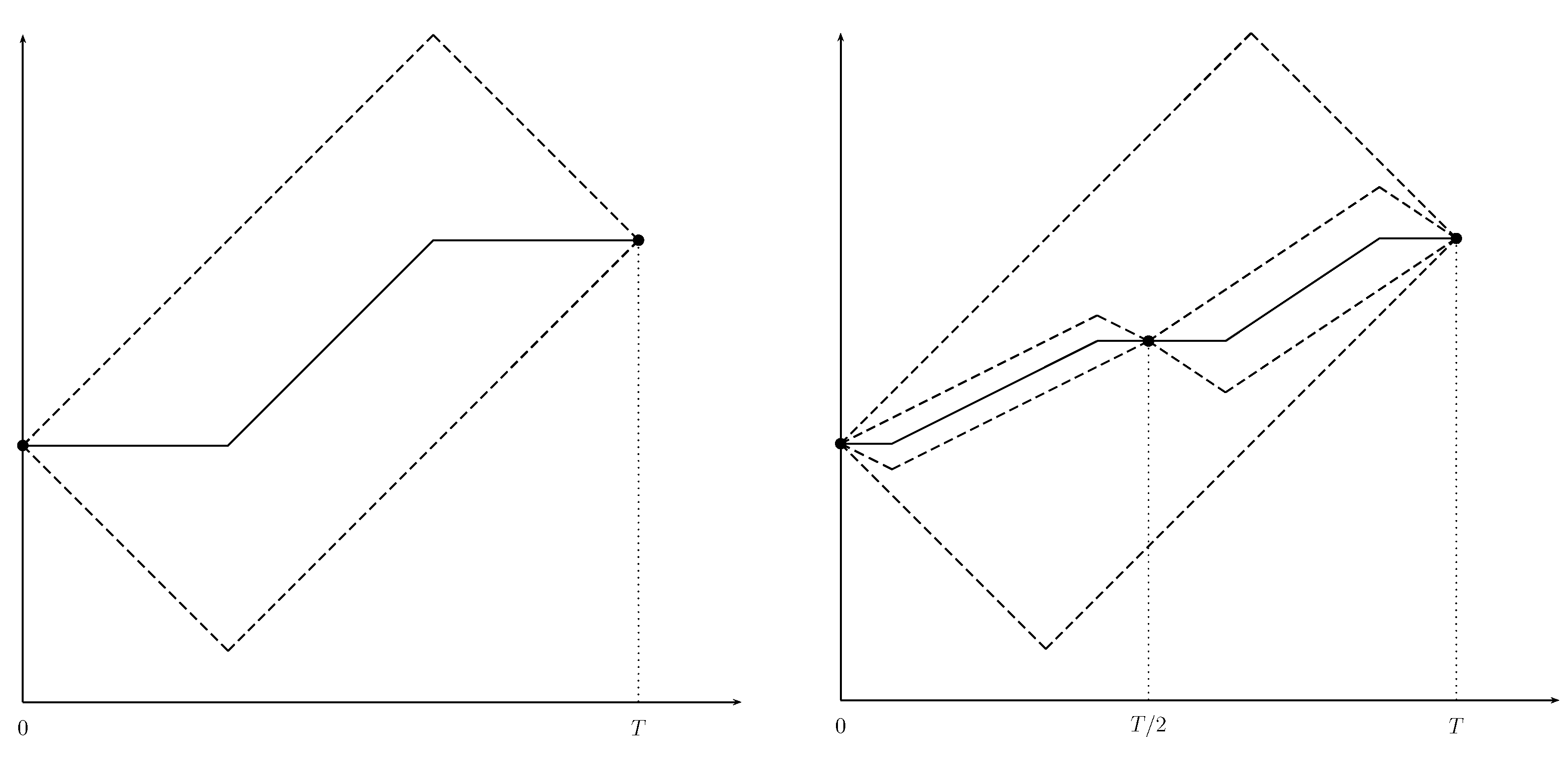
| x j ( t 1 ) x j ( t 2 ) | Λ | t 1 t 2 | , t 1 , t 2 [ 0 , T ] .
Furthermore, let I be the integral of x j over [ 0 , T ] and, to begin with, assume that we only know the value of x j at the two endpoints 0 , T . We wish to construct an approximation of x j in the interval [ 0 , T ] and also obtain an estimate I ^ of the value of I, together with an estimate of the error | I I ^ | .
The Lipschitz continuity of x j allow us to localize its graph by drawing four lines passing trough the points ( 0 , x j ( 0 ) ) and ( T , x j ( T ) ) , with slopes Λ and Λ . We thus construct a parallelogram P 0 , T containing the unknown graph of the function (see Figure 1, left). Specifically, the two upper and the two lower sides of the parallelogram (dashed lines) correspond, respectively, to an upper bound x j u and a lower bound x j l for x j . The functions x j u and x j l can be written as follows:
x j u ( t ) = min { x j ( 0 ) + Λ t , x j ( T ) Λ ( t T ) } , x j l ( x ) = max { x j ( 0 ) Λ t , x j ( T ) + Λ ( t T ) } .
Denote now with x ^ j ( t ) an approximation of the value of x j at some t [ 0 , T ] , with δ ( t ) = | x j ( t ) x ^ j ( t ) | the error on the estimate, and with e w ( t ) = max { x j u ( t ) x ^ j ( t ) , x ^ j ( t ) x j l ( t ) } the largest possible absolute error on the estimate, whence:
δ ( t ) e w ( t ) ,
where the equality sign holds when x j coincides with its upper or lower bound. The case where δ ( t ) = e w ( t ) can be called the worst case, and the value of x ^ j ( t ) that minimizes e w ( t ) is the mean value
x ^ j ( t ) = x j u ( t ) + x j l ( t ) 2 ,
which yields
e w ( t ) = x j u ( t ) x j l ( t ) 2 .
The graph of x ^ j ( t ) , in the worst case, is represented by the solid line in Figure 1, on the left. In order to obtain a global measure of the error in the interval [ 0 , T ] , in the worst case, it is then natural to define:
E w ( 0 , T ) = 0 T e w ( t ) d t = 0 T x j u ( t ) x j l ( t ) 2 d t ,
which is equal to the half of the area of P 0 , T , denoted by A ( 0 , T ) , and thus E w ( 0 , T ) = A ( 0 , T ) / 2 .
We thus have an approximation x ^ j of the function x j , together with the estimates e w and E w of the worst case local and total error, respectively. The average worst case error is defined as E w ( 0 , T ) / T .
We want now to approximate the integral I of x j over [ 0 , T ] . Notice that lower and upper bounds for I are given, respectively, by
I l = 0 T x j l ( t ) d t = ( x j ( 0 ) x j ( T ) ) 2 4 Λ Λ 4 T 2 + T ( x j ( 0 ) + x j ( T ) ) 2 , I u = 0 T x j u ( t ) d t = ( x j ( 0 ) x j ( T ) ) 2 4 Λ + Λ 4 T 2 + T ( x j ( 0 ) + x j ( T ) ) 2 .
The estimate of I that differs the less from the two extreme I l and I u is the average value
I ^ = I l + I u 2 = T ( x j ( 0 ) + x j ( T ) ) 2 .
For this choice of I ^ , the error | I I ^ | can reach the value of E I = ( I u I l ) / 2 in the worst case.
It follows from (17) that I ^ is equal to the integral of the approximating function x ^ j . We remark from (19) that the total worst case error E w coincides with the estimate of the error E I on the integral I ^ . Hence, both for the estimate of the function and of its integral, the quantity that measures the corresponding errors is the same, and it is exactly half the area of the parallelogram P 0 , T . It is easy to check (see [13,14]) that, for any pair of points t 1 , t 2 (with t 1 < t 2 ), the area of parallelogram P t 1 , t 2 is
A ( t 1 , t 2 ) = t 1 t 2 ( x j u ( t ) x j l ( t ) ) d t = Λ 2 ( t 1 t 2 ) 2 ( x j ( t 1 ) x j ( t 2 ) ) 2 2 Λ .
Now, we want to analyze how the evaluation of x j in a further point improves the approximation procedure. For this, let t 1 = 0 , t 2 = T , let t 3 be an arbitrary point in ( 0 , T ) and repeat the previous procedure in the intervals [ 0 , t 3 ] and [ t 3 , T ] , respectively. The graph of x j is now contained in the union of parallelograms P 0 , t 3 and P t 3 , T . Therefore, a new sample point allows to better locate the graph of x j . In this case, the bounding functions are computed as follows:
x j u ( t ) = min { x j ( 0 ) + Λ t , x j ( t 3 ) Λ ( t t 3 ) } i f   t [ 0 , t 3 ] , min { x j ( t 3 ) + Λ ( t t 3 ) , x j ( T ) Λ ( t T ) } i f   t [ t 3 , T ] ,
x j l ( t ) = max { x j ( 0 ) Λ t , x j ( t 3 ) + Λ ( t t 3 ) } i f   t [ 0 , t 3 ] , max { x j ( t 3 ) Λ ( t t 3 ) , x j ( T ) + Λ ( t T ) } i f   t [ t 3 , T ] ,
where Λ and Λ denote the update estimates of the Lipschitz constant of x j in the intervals [ 0 , t 3 ] and [ t 3 , T ] , respectively.
For the two sub-intervals, we can provide approximations of x j and of its integral, and estimates of the corresponding errors E w ( t 1 , t 3 ) and E w ( t 3 , t 2 ) .
We observe that the smaller the sum of the areas of the new parallelograms is, the better the new estimate of the function is. Hence, with the evaluation of x j at new points and repeating the above procedure, we can further improve the approximation x j and its integral, as specified by the following algorithm.
  • Step 0. (Initialization)
    • Fix a positive constant ε t o t , which represents the desired maximum error on the integral of x j (or total worst case error in the estimate of x j itself). Create a list of evaluation points, which initially contains the two endpoints 0 and T, and the corresponding list of function values x j ( 0 ) , x j ( T ) . Calculate the area A ( 0 , T ) of parallelogram P 0 , T by means of (20) and initialize a list of parallelograms’ areas.
  • Step 1. (New evaluation)
    • Locate the parallelogram having the largest area, and the corresponding interval, say [ t 1 , t 2 ] (at the first step, [ t 1 , t 2 ] coincides with the whole interval [ 0 , T ] ). Add the new evaluation point p = ( t 1 + t 2 ) / 2 , and update the lists of points and function values accordingly. Compute the two Lipschitz constants in the intervals [ t 1 , p ] and [ p , t 2 ] . Update the parallelograms’ areas list by removing the area of parallelogram P t 1 , t 2 and inserting the areas of the two new parallelograms P t 1 , p and P p , t 2 .
  • Step 2. (Stopping rule)
    • Compute the worst case error E t o t over the interval [ 0 , T ] :
      E t o t = ( s u m   o f   t h e   a r e a s   o f   a l l   p a r a l l e l o g r a m s ) / 2 .
      If E t o t ε t o t , then stop the procedure, otherwise go to Step 1.
At the k-th iteration of the algorithm, we thus have divided the interval [ 0 , T ] with k + 2 points, which we reorder as { t 1 = 0 , t 2 , , t k + 1 , t k + 2 = T } , and we denote with Λ i the estimate of the Lipschitz constant of x j in [ t i , t i + 1 ] . The bounding functions in [ t i , t i + 1 ] are then given by:
X j u ( t ) | [ t i , t i + 1 ] = min t [ t i , t i + 1 ] x j ( t i ) + Λ i ( t t i ) , x j ( t i + 1 ) Λ i ( t t i + 1 ) , X j l ( t ) | [ t i , t i + 1 ] = max t [ t i , t i + 1 ] x j ( t i ) Λ i ( t t i ) , x j ( t i + 1 ) + Λ i ( t t i + 1 ) .
In the next result, we provide a complexity analysis of the algorithm.
Theorem 4. 
After k iterations of the algorithm, the worst case error E t o t is, at most, equal to
E 0 2 log 2 ( k + 1 ) ,
where
E 0 = Λ 2 T 2 ( x j ( 0 ) x j ( T ) ) 2 4 Λ
is the worst case error before the algorithm starts. Therefore, the algorithm stops after at most 2 E 0 / ε t o t iterations.
Proof. 
At each iteration, we need to compute the two new estimates of the Lipschitz constant in the intervals [ t 1 , p ] and [ p , t 2 ] . Such estimates are less than or equal to the Lipschitz estimate Λ in the interval [ 0 , T ] . Since the area of each parallelogram given by Formula (20) (and thus the error on the integral) is an increasing function of Λ , the worst case occurs when the two estimates coincide with Λ . Hence, the worst case complexity analysis of the algorithm reduces to that of the algorithm where the Lipschitz estimate is not updated at any iteration. Therefore, following the same argument as in [13], we can prove the inequality
A k A 0 1 2 i ,
where A k denotes the sum of the areas of all parallelograms generated by the algorithm after k iterations, A 0 is the area of the parallelogram before the algorithm starts, and i is the integer such that 2 i k + 1 < 2 i + 1 . Since the worst case error E t o t after k iterations is E t o t = A k / 2 , E 0 = A 0 / 2 , and i = log 2 ( k + 1 ) , we obtain the following inequality from (22):
E t o t = A k 2 A 0 / 2 2 i = E 0 2 log 2 ( k + 1 ) ,
thus (21) holds.
If we denote k ¯ = 2 E 0 / ε t o t , then
k ¯ + 1 > 2 E 0 ε t o t 2 E 0 ε t o t ,
thus, we obtain
ε t o t > 2 E 0 k ¯ + 1 = E 0 2 log 2 ( k ¯ + 1 ) 1 E 0 2 log 2 ( k ¯ + 1 ) ,
hence (21) guarantees that the worst case error after k ¯ iterations is less than ε t o t ; that is, the algorithm stops after at most k ¯ iterations. □

4. Application to Parametric Network Games

The theoretical results proved in Section 2 and the approximation algorithm described in Section 3 can be applied to any parametric VI in the form (1). It is well known that parametric VIs in the form (1) can be viewed as the dynamic equilibrium models, in the case where the problem data depend on a time parameter t. Several applications of these models have been studied in recent years (see, e.g., [26,27] and references therein). On the other hand, network games are an interesting class of non-cooperative games with an underlying network structure, which can be modeled through VIs [24]. A number of applications of network games have been analyzed in the literature, from social networks to juvenile delinquency (see, e.g., [20,21] and references therein).
In this section, we apply the results of Section 2 and Section 3 to a class of parametric network games, which can be modeled as parametric VIs in the form (1), where both the players’ utility functions and their strategy sets depend on a time parameter. Specifically, in Section 4.1, a brief recall of Graph Theory and Game Theory concepts is given together with the definition of parametric network games. Then, we focus on the linear-quadratic model, both in the framework of the network Nash equilibrium problem (Section 4.2) and the network generalized Nash equilibrium problem (Section 4.3).

4.1. Basics of Network Games

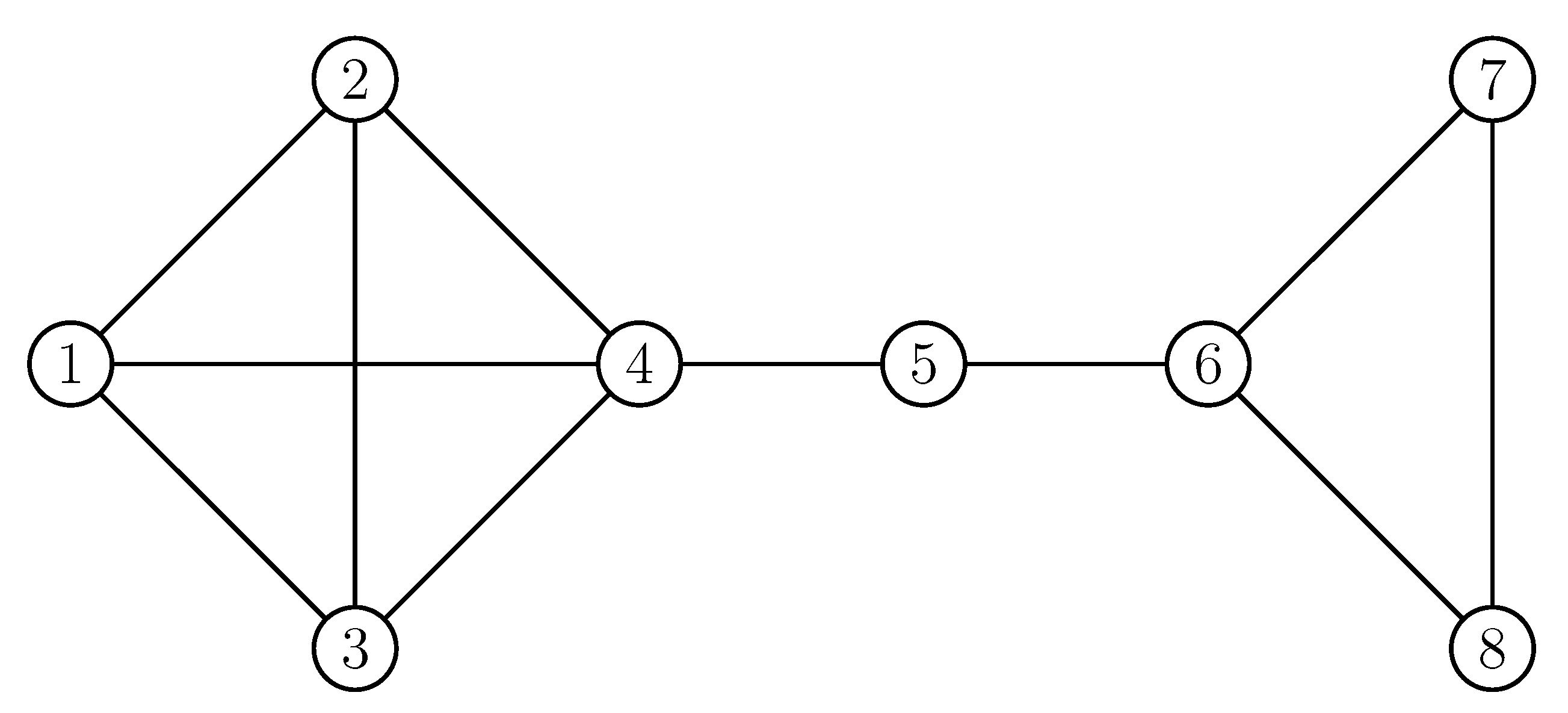
We begin with a recapitulation of foundational Graph Theory concepts. We define a graph g as a pair of sets ( V , E ) , where V represents the set of nodes, while E represents the set of arcs composed of pairs of nodes ( v , w ) . Arcs sharing identical terminal nodes are categorized as parallel arcs, while arcs in the form of ( v , v ) are designated as loops. For the context at hand, we exclusively consider simple graphs, which are characterized by the absence of both parallel arcs and loops. Within our framework, the players are represented by the n nodes of the graph. Furthermore, we operate within the framework of undirected graphs, wherein arcs ( v , w ) and ( w , v ) are considered equivalent. Two nodes v and w are adjacent if they are connected by the arc ( v , w ) . The information regarding the adjacency of nodes can be stored in the form of the adjacency matrix G, where the elements g i j assume a value of 1 when ( v i , v j ) is an arc and 0 otherwise. Notice that matrix G is symmetric and with diagonal elements equal to 0. For a specific node v, the nodes that share a direct link with it through arcs are referred to as the neighbors of v. These neighbors are collated within the set N v ( g ) . The cardinality of N v ( g ) is the degree of v.
A walk is defined as a sequence v 0 , e 1 , v 1 , e 2 , , v k comprising both graph nodes v i and graph edges e i , for any 1 i k , where the arc e i has endpoints v i 1 and v i . Notice that within a walk, the possibility of revisiting a node or traversing an arc multiple times is permitted. The length of a walk is equal to the number of its arcs. The indirect connections between any two nodes within the graph are described through the utilization of the powers of the adjacency matrix G. Indeed, it can be proved that the element g i j [ k ] of G k provides the number of walks of length k between the nodes v i and v j .
We now recall some concepts of Game Theory, which will then be adapted to our specific framework. A strategic game (in normal form) is a model of interaction among decision makers, which are usually called players. Each player has to make a choice among various possible actions, but the outcome of her choice also depends on the choice made by the other players. The elements of the game are:
  • A set of n players;
  • A set A i , for each player i { 1 , , n } , called the strategy (or action) set of player i; each element ( x 1 , x 2 , , x n ) A : = A 1 × A 2 × × A n is called a strategy profile;
  • For each player i { 1 , , n } , a set of preferences, according to which they can order the various profiles;
  • For each player i { 1 , , n } , a utility (or payoff) function, u i : A R , which represents their preferences such that to higher values there correspond better outcomes. Let us notice that the utility function of player i does not merely depend on x i , but on the whole strategy profile x = ( x 1 , x 2 , , x n ) ; that is, the interaction with the other players cannot be neglected in their decision processes.
In the case of more than two players, it is important to distinguish the action of player i from the action of all the other players. To this end, we will use the notation x i to denote the subvector ( x 1 , , x i 1 , x i + 1 , , x n ) , and write x = ( x i , x i ) = ( x 1 , , x n ) . Since each player i wishes to maximize their utility, and only controls her action variable x i , a useful solution concept is that of Nash equilibrium of the game.
Definition 4. 
A Nash equilibrium is a vector x * A such that:
u i ( x i * , x i * ) u i ( x i , x i * ) , i { 1 , , n } , x i A i .
The interested reader can find a comprehensive theoretical treatment of Game Theory in the book [28], along with various applications.
We now adapt the above concepts to our parametric network problem and, for simplicity, still denote the set of players by { 1 , 2 , , n } instead of { v 1 , v 2 , , v n } . Thus, consider an interval [ 0 , T ] , and for each t [ 0 , T ] , denote with A i ( t ) R the parametric strategy space of player i, while A ( t ) = A 1 ( t ) × × A n ( t ) is called the parametric space of action profiles. Each player i is endowed with a payoff function u i : [ 0 , T ] × A ( t ) R that he/she wishes to maximize. The notation u i ( t , x , G ) is often utilized when one wants to emphasize the dependence on the graph structure. We wish to find a Nash equilibrium of the parametric game; that is, for each t [ 0 , T ] , we seek an element x * ( t ) A ( t ) such that for each i { 1 , , n } :
u i ( t , x i * ( t ) , x i * ( t ) ) u i ( t , x i , x i * ( t ) ) , x i A i ( t ) .
A characteristic of network games is that the vector x i is only made up of components x j such that j N i ( g ) ; that is, j is a neighbor of i. For modeling purposes, and also for simplifying the analysis, it is common to make further assumptions on how variations in the actions of a player’s neighbors affect her marginal utility. We assume that the type of interaction does not change in [ 0 , T ] and, in the case where u i ( t , · ) C 2 ( R n ) , we obtain the following definitions.
Definition 5. 
We say that the network game has the property of strategic substitutes if for each player i the following condition holds:
2 u i ( t , x i , x i ) x j x i < 0 , ( i , j ) : g i j = 1 , t [ 0 , T ] , x A ( t ) .
Definition 6. 
We say that the network game has the property of strategic complements if for each player i the following condition holds:
2 u i ( t , x i , x i ) x j x i > 0 , ( i , j ) : g i j = 1 , t [ 0 , T ] , x A ( t ) .
We will use the variational inequality approach, pioneered by [23] (in the non-parametric case), to solve Nash equilibrium problems. If, for each t [ 0 , T ] , the u i are continuously differentiable functions on R n , and u i ( t , · , x i ) are concave, the Nash equilibrium problem is equivalent to the variational inequality V I ( F , A ( t ) ) :
For each t [ 0 , T ] , find x * ( t ) A ( t ) such that
F ( t , x * ( t ) ) , x x * ( t ) 0 , x A ( t ) ,
where
[ F ( t , x ) ] : = u 1 x 1 ( t , x ) , , u n a n ( t , x )
is also called the pseudo-gradient of the game, according to the terminology introduced by Rosen [29].
In the following subsection, we introduce the parametric linear-quadratic utility functions, which will be used both for the Nash equilibrium problem and the generalized Nash equilibrium problem. This simple functional form as been extensively used in the literature (see, e.g, [20]) because, in the case on non-negative strategy space, it allows solutions in closed form. We consider instead the case where the strategy space of each player has a (parameter-dependent) upper bound.

4.2. The Linear-Quadratic Network Nash Equilibrium Problem

Let A i ( t ) = [ 0 , U i ( t ) ] for any i { 1 , , n } , t [ 0 , T ] , where, for each i, U i ( t ) is a positive and Lipschitz continuous function on [ 0 , T ] . The payoff of player i is given by:
u i ( t , x ) = k ( t ) x i 1 2 x i 2 + ϕ j = 1 n g i j x i x j ,
In this model k : [ 0 , T ] R is a positive Lipschitz function, and ϕ > 0 describes the interaction between a player and their neighbors, which corresponds to the case of strategic complements. Moreover, since k ( t ) is the same for all players, they only differ because of their position in the network. The pseudo-gradient’s components are given by:
F i ( t , x ) = k ( t ) + x i ϕ j = 1 n g i j x j , i { 1 , , n } ,
which can be written in compact form as:
F ( t , x ) = ( I ϕ G ) x k ( t ) 1 ,
where 1 = ( 1 , , 1 ) R n . We will seek Nash equilibrium points by solving the variational inequality: for each t [ 0 , T ] , find x * ( t ) A ( t ) such that
( I ϕ G ) x * ( t ) k ( t ) 1 , x x * ( t ) 0 , x A ( t ) .
Lemma 1. 
F is uniformly strongly monotone if ϕ ρ ( G ) < 1 , where ρ ( G ) is the spectral radius of G.
Proof. 
The symmetric matrix I ϕ G is positive definite if and only if its minimum eigenvalue λ m i n ( I ϕ G ) is positive. On the other hand, λ m i n ( I ϕ G ) = 1 ϕ λ m a x ( G ) . Since G is a symmetric non-negative matrix, the Perron–Frobenius Theorem guarantees that λ m a x ( G ) = ρ ( G ) , hence I ϕ G is positive definite if and only if ϕ ρ ( G ) < 1 . This condition does not depend on t [ 0 , T ] . □
Notice that, when ϕ ρ ( G ) < 1 , the map F in (28) satisfies the assumptions of Theorems 2 and 3 with constants α = 1 ϕ ρ ( G ) , L x = I ϕ G 2 , L t = L k n , where L k is the Lipschitz constant of k ( t ) , and L = max { L x , L t } . Moreover, the feasible region A ( t ) satisfies assumption (3) with constant M = ( L 1 , , L n ) 2 , where L i is the Lipschitz constant of U i ( t ) for any i = 1 , , n (see [11]). Therefore, it follows from Theorems 2 and 3 that the Nash equilibrium x * ( t ) is a Lipschitz continuous function with estimated constant equal to min { Λ 1 , Λ 2 } .
Remark 1. 
The game under consideration also falls, for each t [ 0 , T ] , in the class of potential games according to the definition introduced by Monderer and Shapley [30]. Indeed, a potential function is given by:
P ( t , x ) = i = 1 n u i ( t , x ) ϕ 2 i = 1 n j = 1 n g i j x i x j .
Monderer and Shapley have proven that, in general, the solutions of the problem
max x A ( t ) P ( t , x )
form a subset of the solution set of the Nash game. Because both problems have a unique solution under the condition ϕ ρ ( G ) < 1 , it follows that the two problems share the same solution.

4.3. The Linear-Quadratic Network Generalized Nash Equilibrium Problem

We start this subsection with a recall of generalized Nash equilibrium problems (GNEPs) with shared constraints and their variational solutions. More details can be found in the already-mentioned paper by Rosen, and in the more recent papers [31,32,33,34,35,36,37,38]. We directly introduce the parametric case, and all the following definitions and properties hold for any fixed t [ 0 , T ] .
In GNEPs, the strategy set of each player is dependent on the strategies of their rivals. In this context, we examine a simplified scenario where the variable x is constrained to be non-negative ( x 0 ). Moreover, we consider a function g : [ 0 , T ] × R n R m , which characterizes the collective constraints shared among the players. For each t, and for each move x i of the other players, the strategy set of player i is then given by:
K i ( t , x i ) = { x i R + : g ( t , x ) = g ( t , x i , x i ) 0 } .
Definition 7. 
The GNEP is the problem of finding, for each t [ 0 , T ] , x * ( t ) R n such that, for any i { 1 , , n } , x i * ( t ) K i ( t , x i * ( t ) ) and
u i ( t , x i * ( t ) , x i * ( t ) ) u i ( x i , x i * ( t ) ) , t [ 0 , T ] , x i K i ( t , x i * ( t ) ) .
We assume that that, for each fixed t [ 0 , T ] , x i K i ( t , x i * ) , the functions u i ( t , · , x i ) are concave and continuously differentiable, and the components of g ( t , · ) are convex and continuously differentiable. As a consequence, a necessary and sufficient condition for x i * ( t ) K i ( t , x i * ) to satisfy (31) is
u i ( t , x i * ( t ) , x i * ( t ) ) x i ( x i x i * ( t ) ) 0 , t [ 0 , T ] , x i K i ( t , x i * ( t ) ) .
Thus, if we define F ( t , x ) as in (26), and
K ( t , x ) = K 1 ( t , x 1 ) × × K n ( t , x n ) ,
it follows that x * ( t ) is a GNE if and only if, t [ 0 , T ] , x * ( t ) K ( t , x * ( t ) ) and
F ( t , x * ( t ) ) , x x * ( t ) 0 , x K ( t , x * ( t ) ) .
The above problem, where the feasible set also depends on the solution, is called a quasi-variational inequality (with parameter t), and its solution is as difficult as the original GNEP. Let us now remark that even if the strict monotonicity assumption on F is satisfied for each t, the above problem (equivalent to the original GNEP) has infinite solutions. We can select a specific solution by studying its Lagrange multipliers.
Thus, assume that, for each t [ 0 , T ] , x * ( t ) is a solution of GNEP. Hence, for each i, x i * ( t ) solves the maximization problem
max x i { u i ( t , x i , x i * ( t ) ) : g ( t , x i , x i * ( t ) ) 0 , x i 0 } .
Under some standard constraint qualification, we can then write the KKT conditions for each maximization problem. We then introduce the Lagrange multiplier λ i ( t ) R m associated with the constraint g ( t , x i , x i * ) 0 and the multiplier μ i ( t ) R associated with the nonnegativity constraint x i 0 . The Lagrangian function for each player i reads as:
L i ( t , x i , x i * ( t ) , λ i ( t ) , μ i ( t ) ) = u i ( t , x i , x i * ( t ) ) g ( t , x i , x i * ( t ) ) , λ i ( t ) + μ i ( t ) x i
and the KKT conditions for all players are given by:
x i L i ( t , x i * ( t ) , x i * ( t ) , λ i * ( t ) , μ i * ( t ) ) = 0 , i = 1 , , n ,
λ j i * ( t ) g j ( t , x * ( t ) ) = 0 , λ j i * ( t ) 0 , g j ( t , x * ( t ) ) 0 , i = 1 , , n , j = 1 , , m
μ i * ( t ) x i * ( t ) = 0 , μ i * ( t ) 0 , x i * ( t ) 0 , i = 1 , , n .
Conversely, under the assumptions made, if, for any fixed t, ( x * ( t ) , λ ( t ) , μ * ( t ) ) , where λ * ( t ) = ( λ 1 * ( t ) , , λ n * ( t ) ) and μ * ( t ) = ( μ 1 * ( t ) , , μ n * ( t ) ) , satisfy the KKT system (34)–(36), then x * ( t ) is a GNE. We are now in position to classify equilibria.
Definition 8. 
Let x * ( t ) be a GNE which, together with the Lagrange multipliers λ * ( t ) = ( λ 1 * ( t ) , , λ n * ( t ) ) and μ * ( t ) = ( μ 1 * ( t ) , , μ n * ( t ) ) , satisfies the KKT system of all players. We call x * ( t ) a normalized equilibrium if there exists a vector r ( t ) R + + n and a vector λ ¯ ( t ) R + m such that
λ i * ( t ) = λ ¯ ( t ) r i ( t ) , i = 1 , , n ,
which means that, for a normalized equilibrium, the multipliers of the constraints shared by all players are proportional to a common multiplier. In the special case where, for some t, r i ( t ) = 1 for any i, i.e., the multipliers coincide for each player, x * ( t ) is calledvariational equilibrium (VE). Rosen [29] proved that if the feasible set, which in our case is:
K ( t ) = { x R + n : g ( t , x ) 0 }
is compact and convex, then there exists a normalized equilibrium for each r ( t ) R + + n .
Now, let us define, for each r ( t ) R + + n , the vector function F r ( t ) : R n R n as follows:
[ F r ( t ) ( t , x ) ] : = r 1 ( t ) u 1 x 1 ( t , x ) , , r n ( t ) u n x n ( t , x ) .
The variational inequality approach for finding the normalized equilibria of the GNEP is expressed by the following theorem, which can be viewed as a special case of Proposition 3.2 in [34] in a parametric setting.
Theorem 5. 
1. 
Suppose that x * ( t ) is a solution of V I ( F r ( t ) , K ( t ) ) , where r ( t ) R + + n , a constraint qualification holds at x * ( t ) and ( λ ¯ ( t ) , μ ¯ ( t ) ) R m × R n are the multipliers associated with x * ( t ) . Then, x * ( t ) is a normalized equilibrium such that the multipliers ( λ i * ( t ) , μ i * ( t ) ) of each player i satisfy the following conditions:
λ i * ( t ) = λ ¯ ( t ) r i ( t ) , μ i * ( t ) = μ ¯ i ( t ) r i ( t ) , i = 1 , , n .
2. 
If x * ( t ) is a normalized equilibrium such that the multipliers ( λ i * ( t ) , μ i * ( t ) ) of each player i satisfy the following conditions:
λ i * ( t ) = λ ¯ ( t ) r i ( t ) , i = 1 , , n ,
for some vector λ ¯ ( t ) R + m and r ( t ) R + + n , then x * ( t ) is a solution of V I ( F r ( t ) , K ( t ) ) and ( λ ¯ ( t ) , r 1 ( t ) μ 1 * ( t ) , , r n ( t ) μ n * ( t ) ) are the corresponding multipliers.
The variational equilibria can then be computed by solving, for any t [ 0 , T ] , the following variational inequality: find x * ( t ) K ( t ) such that
F ( t , x * ( t ) ) , x x * ( t ) 0 , x K ( t ) .
As an example of network GNEP, we consider the same payoff functions defined as in (27), while the strategy set of player i is given by the usual individual constraint x i 0 and an additional constraint, shared by all the players, on the total quantity of activities of all players, that is
K i ( t , x i ) = x i R + : i = 1 n x i C ( t ) , i = 1 , , n , t [ 0 , T ] ,
where C : [ 0 , T ] R is a given positive and Lipschitz continuous function. Depending on the specific application, the additional constraint can have the meaning of a collective budget upper bound or of a limited availability of a certain commodity. If ϕ ρ ( G ) < 1 , then the variational equilibrium can thus be found by solving V I ( F , K ( t ) ) , where F is the same as in (28) and
K ( t ) = x R + n : i = 1 n x i C ( t ) .
Notice that K ( t ) satisfies Assumption (3), with constant M equal to the Lipschitz constant of the function C (see [11]). Therefore, Theorems 2 and 3 guarantee that the variational equilibrium x * ( t ) is a Lipschitz continuous function with estimated constant equal to min { Λ 1 , Λ 2 } .

5. Numerical Experiments

In this section, some numerical experiments show the performance of the algorithm described in Section 3 based on the new Lipschitz estimates provided in Section 2.
First, we compare the new Lipschitz estimate Λ 1 provided in Theorem 2 with that provided in [12] from the numerical point of view on a set of sample parameters. Then, we compare the performance of the algorithm described in Section 3 based on the Lipschitz estimate used. The algorithm and the computation of Lipschitz estimates were implemented in MATLAB R2023a.

5.1. Comparison between Λ 1 and the Estimate in [12]

Under the same assumptions of Theorem 2, the authors in [12] proved that the solution x ( t ) of the V I ( F , K ( t ) ) is Lipschitz continuous with a constant equal to
Λ 0 = inf ( ε , λ ) M + λ 2 + λ ε + λ 2 1 1 + λ 2 ( 1 + ε ) λ ( 2 α ˜ ε ) : 0 < ε < 2 α ˜ , 0 < λ ( 1 + ε ) + ε < 2 α ˜ ,
where α ˜ = α / L . Since it is not easy to write the estimates Λ 0 and Λ 1 in closed form, we decided to compare them numerically. We considered the following grid for the parameters ( α ˜ , M ) : α ˜ varies from 0.01 to 1 with a step equal to 0.01, while M varies from 0 to 10 with step equal to 0.01. For any value of ( α ˜ , M ) in the considered grid, we computed the values of Λ 0 and Λ 1 : the minimum value in Λ 0 was numerically approximated (due to the non-convexity of the objective function and constraints), while the minimum value in Λ 1 was computed by exploiting the MATLAB function fminbnd. The results show that the new estimate Λ 1 definitely improves Λ 0 . In fact, Λ 1 is always less than Λ 0 and the relative improvement in Λ 1 compared to Λ 0 , i.e., ( Λ 0 Λ 1 ) / Λ 0 , is about 42 % on average with a minimum of 13 % and a maximum of 99 % .

5.2. Performance of the Algorithm

We now show the performance of the algorithm described in Section 3 to solve a linear-quadratic network Nash equilibrium problem (Example 1) and a linear-quadratic network GNEP (Example 2). We implemented three different versions of the algorithm according to the Lipschitz estimate used. We considered the estimate Λ 0 provided in [12], and the new estimates Λ 1 and Λ 2 introduced in Theorems 2 and 3, respectively.
Example 1. 
We consider a linear-quadratic network Nash equilibrium problem as in the framework of Section 4.2, with a network of 8 nodes (players) as shown in Figure 2.
The spectral radius of the adjacency matrix G is ρ ( G ) 3.1019 . We set the function k ( t ) = t + 5 , with t [ 0 , 15 ] . We set two different values for parameter ϕ: ϕ = 0.1 / ρ ( G ) or ϕ = 0.5 / ρ ( G ) , so that there exists a unique Nash equilibrium in both cases. We set the upper bounds U i ( t ) = min { 2 i + ( t + 5 ) / 2 , 18 } for any i = 1 , , 8 . We recall that the map F in (28) satisfies the assumptions of Theorems 2 and 3 with constants α = 1 ϕ ρ ( G ) , L x = I ϕ G 2 , L t = 8 , L = max { L x , L t } , and the feasible region
A ( t ) = i = 1 8 [ 0 , U i ( t ) ]
satisfies Assumption (3) with constant M = ( L 1 , , L 8 ) 2 , where L i is the Lipschitz constant of the function U i for any i = 1 , , 8 . We run the algorithm to approximate the fifth component of the solution vector x ( t ) , due to the special position of the player 5 in the network. To evaluate the function x 5 ( t ) during the execution of the algorithm, i.e., to find Nash equilibria of the problem, we exploited the ad hoc algorithm proposed in [39].
Table 2 shows the number of iterations performed (or Nash equilibria computed) by the three versions of the algorithm (based on the estimates Λ 0 , Λ 1 and Λ 2 ) for different values of ϕ and the error tolerance ε t o t . We set the maximum number of iterations equal to 10 6 . Results show that the algorithm based on the estimate Λ 2 outperforms the other two versions based on the estimates Λ 0 and Λ 1 . Table 3 shows the convergence of the approximate mean value of x 5 ( t ) (computed by the algorithm based on Λ 2 ) for different values of ϕ.
Moreover, we run the algorithm to solve the problem in the case the feasible region A ( t ) is constant, with U i ( t ) = 18 for any t and i = 1 , , 8 , and the map F is the same as before. Table 4 and Table 5 show the number of iterations of the algorithm and the approximate mean value of x 5 ( t ) , respectively. Notice that, in this case, the Lipschitz estimates Λ 1 and Λ 2 coincide, since L = L t and the algorithm based on such an estimate is much more efficient than the one based on Λ 0 .
Example 2. 
We now consider a linear-quadratic network generalized Nash equilibrium problem, as in the framework of Section 4.3. We assume that the player network is the same as Example 1. We set the function k ( t ) = t + 5 , with t [ 0 , 15 ] , ϕ = 0.1 / ρ ( G ) or ϕ = 0.5 / ρ ( G ) , and K ( t ) defined as in (38) with C ( t ) = min { 13 + t , 18 } . The map F in (28) satisfies the assumptions of Theorems 2 and 3 with constants α = 1 ϕ ρ ( G ) , L x = I ϕ G 2 , L t = 8 , L = max { L x , L t } , and the feasible region satisfies assumption (3) with constant M = 1 . In order to find the unique variational equilibrium x ( t ) of the problem, we found the maximizer of the potential function (30) by means of the MATLAB functionquadprog. As in Example 1, we run the algorithm to approximate the fifth component of the solution vector x ( t ) .
Table 6 shows the number of iterations performed by the three versions of the algorithm (based on the estimates Λ 0 , Λ 1 and Λ 2 ) for different values of ϕ and ε t o t . Results show again that the algorithm based on the estimate Λ 2 outperforms the other two versions based on the estimates Λ 0 and Λ 1 . Table 7 shows the convergence of the approximate mean value of x 5 ( t ) for different values of ϕ.
Similarly to Example 1, Table 8 and Table 9 show the number of iterations of the algorithm and the approximate mean value of x 5 ( t ) in the case where the feasible region K ( t ) is constant, with C ( t ) = 18 for any t, and the map F is the same as before.

6. Conclusions

In this paper, we improved previous estimates of the global Lipschitz constant of the unique solution of a parametric variational inequality. Having in mind various applications where the parameter represents time, we utilized the estimated constant to approximate the mean value of the solution by modifying an algorithm previously derived to approximate black box Lipschitz functions. We then applied our results to two class of games played on networks, where we assumed that some terms of the players’ utility functions as well as the constraint set could vary with time. In future work, we plan to investigate the case where also the adjacency matrix of the graph is time-dependent.

Author Contributions

M.P. and F.R. have contributed equally to this work. All authors have read and agreed to the published version of the manuscript.

Funding

This research was partially supported by the research project “Programma ricerca di ateneo UNICT 2020-22 linea 2-OMNIA” of the University of Catania. This support is gratefully acknowledged.

Data Availability Statement

The data presented in this study are available in the article.

Acknowledgments

The authors are members of the Gruppo Nazionale per l’Analisi Matematica, la Probabilità e le loro Applicazioni (GNAMPA—National Group for Mathematical Analysis, Probability and their Applications) of the Instituto Nazionale di Alta Matematica (INdAM—National Institute of Higher Mathematics).

Conflicts of Interest

The authors declare no conflict of interest.

Appendix A

Appendix A.1. Special Case α ˜ = 1 in Theorem 2

The function
f ( z ) = M z + 1 + z 1 z
is strictly convex in ( 0 , 1 ) and
f ( z ) = 2 z 2 M z 2 + 2 M z M z 2 ( 1 z ) 2 .
If M = 0 , then inf z ( 0 , 1 ) f ( z ) = 1 . If M > 0 , then the minimizer of f is
z ¯ = M + 2 M 2 M i f M < 2 , 1 2 i f M = 2 , M 2 M M 2 i f M > 2 .
Therefore, we have
inf z ( 0 , 1 ) f ( z ) = 7 i f M = 2 , M 2 M M 2 M + 1 + 2 M M 2 M 1 2 M M 2 M i f M 2 , = 7 i f M = 2 , 1 + M + 2 2 M i f M 2 , = 1 + M + 2 2 M .
The function
f ( z ) = M 2 z + z ( 1 + z ) ( z 1 ) ( 2 z ) = z 2 + z ( M + 1 ) M z 2 + 3 z 2
is strictly convex in ( 1 , 2 ) and
f ( z ) = ( 4 + M ) z 2 2 z ( M + 2 ) + M 2 ( z 2 + 3 z 2 ) 2 .
Thus, the minimum is reached in
z ¯ = M + 2 + 2 M + 12 M + 4 ,
which belongs to the interval ( 1 , 2 ) . Therefore, we have
inf z ( 1 , 2 ) f ( z ) = 4 M + 24 + ( M 2 + 7 M + 8 ) 2 M + 12 ( M + 8 ) 2 M + 12 4 M 24 = 8 M + 6 + M 2 + 7 M + 8 M + 8 8 M + 6 = M 2 + 7 M + 8 + 2 2 M + 12 M + 8 2 2 M + 12 .

Appendix A.2. Special Case α ˜ = 1 in Theorem 3

The function
f ( z ) = M z + L ^ 1 + z 1 z
is strictly convex in ( 0 , 1 ) and
f ( z ) = 2 L z 2 M ( 1 z ) 2 z 2 ( 1 z ) 2 .
If M = 0 , then inf z ( 0 , 1 ) f ( z ) = L ^ . If M > 0 , then the minimizer of f is
z ¯ = M + 2 L ^ M 2 L ^ M i f   2 L ^ M > 0 , M + 2 L ^ M 2 L ^ M i f   2 L ^ M < 0 , 1 2 i f   2 L ^ M = 0 .
Therefore, we have
inf z ( 0 , 1 ) f ( z ) = 7 L ^ i f   M = 2 L ^ , M ( 2 L ^ M = 2 L ^ M M + L ^ 1 + 2 L ^ M M 2 L ^ M 1 2 L ^ M M 2 L ^ M i f   M 2 L ^ , = 7 L ^ i f   M = 2 L ^ , M + 2 2 L ^ M + L ^ i f   M 2 L ^ , = M + 2 2 L ^ M + L ^ .
The function
f ( z ) = M 2 z + L ^ z ( 1 + z ) ( z 1 ) ( 2 z ) = L ^ z 2 + z ( M + L ^ ) M z 2 + 3 z 2
is strictly convex in ( 1 , 2 ) and
f ( z ) = ( 4 L ^ + M ) z 2 2 ( 2 L ^ + M ) z + M 2 L ^ ( z 2 + 3 z 2 ) 2 .
The minimum point is
z ¯ = M + 2 L ^ + 2 L ^ M + 12 L ^ 2 4 L ^ + M
which belongs to ( 1 , 2 ) . Moreover, after some algebra, we obtain:
inf z ( 1 , 2 ) f ( z ) = ( M 2 + 7 L ^ M + 8 L ^ 2 ) 12 L ^ 2 + 2 L ^ M + 4 M L ^ 2 + 24 L ^ 3 ( M + 8 L ^ ) 12 L ^ 2 + 2 L ^ M 4 L ^ M 24 L ^ 2 = M 2 + 7 L ^ M + 8 L ^ 2 + L ^ 8 L ^ M + 6 L ^ M + 8 L ^ 8 L ^ M + 6 L ^ = M 2 + 7 M L ^ + 8 L ^ 2 + 2 L ^ 2 M L ^ + 12 L ^ 2 M + 8 L ^ 2 2 M L ^ + 12 L ^ 2 .

References

  1. Bank, B.; Guddat, J.; Klatte, D.; Kummer, B.; Tammer, K. Non-Linear Parametric Optimization; Springer: Berlin/Heidelberg, Germany, 1983. [Google Scholar]
  2. Aubin, J.-P. Lipschitz behavior of solutions to convex minimization problems. Math. Oper. Res. 1984, 9, 87–111. [Google Scholar] [CrossRef]
  3. Mansour, M.A.; Bahraoui, M.A.; Adham, E.B. Approximate solutions of quasi-equilibrium problems: Lipschitz dependence of solutions on parameters. J. Appl. Numer. Optim. 2021, 3, 297–314. [Google Scholar]
  4. Li, W. The sharp Lipschitz constants for feasible and optimal solutions of a perturbed linear program. Linear Algebra Appl. 1993, 187, 15–40. [Google Scholar] [CrossRef]
  5. Li, W. Sharp Lipschitz constants for basic optimal solutions and basic feasible solutions of linear programs. SIAM J. Control Optim. 1994, 32, 140–153. [Google Scholar] [CrossRef]
  6. Klatte, D.; Gisbert, T. A note of Lipschitz constants for solutions of linear inequalities and equations. Linear Algebra Appl. 1996, 244, 365–374. [Google Scholar] [CrossRef]
  7. Mangasarian, O.L.; Shiau, T.H. Lipschitz continuity of solutions of linear inequalities, programs and complementarity problems. SIAM J. Control Optim. 1986, 25, 583–595. [Google Scholar] [CrossRef]
  8. Facchinei, F.; Pang, J.-S. Finite-Dimensional Variational Inequalities and Complementarity Problems; Springer: Berlin, Germany, 2003. [Google Scholar]
  9. Yen, N.D. Lipschitz Continuity of Solutions of Variational Inequalities with a Parametric Polyhedral Constraint. Math. Oper. Res. 1995, 20, 695–708. [Google Scholar] [CrossRef]
  10. Maugeri, A.; Scrimali, L. Global Lipschitz Continuity of Solutions to Parameterized Variational Inequalities. Boll. Dell’Unione Mat. Ital. 2009, 2, 45–69. [Google Scholar]
  11. Causa, A.; Raciti, F. Lipschitz Continuity Results for a Class of Variational Inequalities and Applications: A Geometric Approach. J. Optim. Theory Appl. 2010, 145, 235–248. [Google Scholar] [CrossRef]
  12. Falsaperla, P.; Raciti, F. Global Approximation of Solutions of Time-Dependent Variational Inequalities. Numer. Funct. Anal. Optim. 2014, 35, 1018–1042. [Google Scholar] [CrossRef]
  13. Zabinsky, Z.B.; Smith, R.L.; Kristinsdottir, B.P. Optimal estimation of univariate black-box Lipschitz functions with upper and lower error bounds. Comput. Oper. Res. 2003, 30, 1539–1553. [Google Scholar] [CrossRef]
  14. Baran, I.; Demain, E.D.; Katz, D.A. Optimally Adaptive Integration of Univariate Lipschitz Functions. Algorithmica 2008, 50, 255–278. [Google Scholar] [CrossRef]
  15. Ballester, C.; Calvo-Armengol, A.; Zenou, Y. Who’s Who in Networks. Wanted: The Key Player. Econometrica 2006, 74, 1403–1417. [Google Scholar] [CrossRef]
  16. Belhaj, M.; Bramoulleé, Y.; Deroian, F. Network games under strategic complementarities. Games Econon. Behav. 2014, 88, 310–319. [Google Scholar] [CrossRef]
  17. Calvo-Armengol, A.; Patacchini, E.; Zenou, Y. Peer effects and social networks in education. Rev. Econ. Stud. 2009, 76, 1239–1267. [Google Scholar] [CrossRef]
  18. Helsley, R.; Zenou, Y. Social networks and interactions in cities. J. Econ. Theory 2014, 150, 426–466. [Google Scholar] [CrossRef]
  19. Liu, X.; Patacchini, E.; Zenou, Y. Endogenous peer effects: Local aggregate or local average? J. Econ. Behav. Organ. 2014, 103, 39–59. [Google Scholar] [CrossRef]
  20. Jackson, M.O.; Zenou, Y. Games on Networks. In Handbook of Game Theory with Economic Applications; Elsevier: Amsterdam, The Netherlands, 2015; pp. 95–163. [Google Scholar]
  21. Goyal, S. Connections: An Introduction to the Economics of Networks; Princeton University Press: Princeton, NJ, USA, 2007. [Google Scholar]
  22. Bonacich, P. Power and centrality: A family of measures. Am. J. Sociol. 1987, 92, 1170–1182. [Google Scholar] [CrossRef]
  23. Gabay, D.; Moulin, H. On the uniqueness and stability of Nash equilibria in noncooperative games. In Applied Stochastic Control in Econometrics and Management Science; Bensoussan, A., Kleindorfer, P., Tapiero, C.S., Eds.; North-Holland: Amsterdam, The Netherlands, 1980; pp. 271–294. [Google Scholar]
  24. Parise, F.; Ozdaglar, A. A variational inequality framework for network games: Existence, uniqueness, convergence and sensitivity analysis. Games Econ. Behav. 2019, 114, 47–82. [Google Scholar] [CrossRef]
  25. Passacantando, M.; Raciti, F. A note on generalized Nash games played on networks. In Nonlinear Analysis, Differential Equations, and Applications; Rassias, T.M., Ed.; Optimization and Its Applications; Springer: Berlin/Heidelberg, Germany, 2021; Volume 173, pp. 365–380. [Google Scholar]
  26. Daniele, P. Dynamic Networks and Evolutionary Variational Inequalities; Edward Elgar Publishing: Cheltenham, UK, 2006. [Google Scholar]
  27. Pang, J.-S.; Stewart, D.E. Differential variational inequalities. Math. Program. 2008, 113, 345–424. [Google Scholar] [CrossRef]
  28. Osborne, M.J. Introduction to Game Theory: International Edition; OUP Catalogue; Oxford University Press: Oxford, UK, 2009. [Google Scholar]
  29. Rosen, J.B. Existence and uniqueness of equilibrium points for concave n person games. Econometrica 1965, 33, 520–534. [Google Scholar] [CrossRef]
  30. Monderer, D.; Shapley, L.S. Potential games. Games Econ. Behav. 1996, 14, 124–143. [Google Scholar] [CrossRef]
  31. Facchinei, F.; Fischer, A.; Piccialli, V. On generalized Nash games and variational inequalities. Oper. Res. Lett. 2007, 35, 159–164. [Google Scholar] [CrossRef]
  32. Facchinei, F.; Kanzov, C. Generalized Nash equilibrium problems. Ann. Oper. Res. 2010, 175, 177–211. [Google Scholar] [CrossRef]
  33. Nabetani, K. Variational Inequality Approaches to Generalized Nash Equilibrium Problems. Master’s Thesis, Department of Applied Mathematics and Physics Graduate School of Informatics, Kyoto University, Kyoto, Japan, 2008. [Google Scholar]
  34. Nabetani, K.; Tseng, P.; Fukushima, M. Parametrized variational inequality approaches to generalized Nash equilibrium problems with shared constraints. Comput. Optim. Appl. 2011, 48, 423–452. [Google Scholar] [CrossRef]
  35. Nagurney, A.; Alvarez Flores, E.; Soylu, C. A Generalized Nash Equilibrium network model for post-disaster humanitarian relief. Transp. Res. E Logist. Transp. Rev. 2016, 95, 1–18. [Google Scholar] [CrossRef]
  36. Aussel, D.; Dutta, J. Generalized Nash equilibrium problem, variational inequality and quasiconvexity. Oper. Res. Lett. 2011, 36, 461–464. [Google Scholar] [CrossRef]
  37. Aussel, D.; Cao Van, K.; Salas, D. Existence Results for Generalized Nash Equilibrium Problems under Continuity-Like Properties of Sublevel Sets. Siam J. Optim. 2021, 31, 2784–2806. [Google Scholar] [CrossRef]
  38. Krilašević, S.; Grammatico, S. Learning generalized Nash equilibria in multi-agent dynamical systems via extremum seeking control. Automatica 2021, 133, 109846. [Google Scholar] [CrossRef]
  39. Passacantando, M.; Raciti, F. A finite convergence algorithm for solving linear-quadratic network games with strategic complements and bounded strategies. Optim. Methods Softw. 2023, 1–24. [Google Scholar] [CrossRef]
Figure 1. Upper and lower bounds (dashed lines) and best approximation (solid line) of a Lipschitz continuous function evaluated at t = 0 and t = T (left), and same curves after the evaluation at the midpoint t = T / 2 .
Algorithms 16 00458 g001
Figure 2. Network topology of Example 1.
Algorithms 16 00458 g002
Table 1. Estimate of the Lipschitz constant of x ( t ) depending on the features of the map F and the feasible set K.
General KConstant K
General F Λ 1 = inf z 0 , 2 α ˜ M 1 s + z ( 1 + z ) s ( 1 s ) , if α ˜ < 1 , M + 2 2 M + 1 , if α ˜ = 1 , Λ 1 = L α
where α ˜ = α L , s = z 2 2 α ˜ z + 1
Separable F Λ 2 = inf z 0 , 2 α ^ M 1 s ^ + L ^ z ( 1 + z ) s ^ ( 1 s ^ ) , if α ^ < 1 , M + 2 2 M L ^ + L ^ , if α ^ = 1 , Λ 2 = L t α
where α ^ = α L x , L ^ = L t L x , s ^ = z 2 2 α ^ z + 1
Constant F Λ 2 = M 1 1 α L 2
Table 2. Example 1 with a moving feasible region: number of iterations of the algorithm based on the Lipschitz estimate used.
ϕ = 0.1 / ρ ( G ) ϕ = 0.5 / ρ ( G )
ε tot Alg with   Λ 0 Alg with  Λ 1 Alg with   Λ 2 Alg with   Λ 0 Alg with   Λ 1 Alg with  Λ 2
15107179964015,38352461714
0.510,2133597127730,76510,4903426
0.226,0698554326078,85826,4317995
0.152,13617,1076518157,71552,86015,989
0.05104,27034,21213,034315,428105,71931,977
0.02246,32192,25030,788815,228249,97685,721
0.01492,640184,49961,575>1 × 10 6 499,950171,441
Lipschitz
estimate
Λ 0 = 88.46 Λ 1 = 33.18 Λ 2 = 11.18 Λ 0 = 276.49 Λ 1 = 96.82 Λ 2 = 30.31
Table 3. Example 1 with a moving feasible region: approximate mean value of x 5 ( t ) .
ε tot ϕ = 0.1 / ρ ( G ) ϕ = 0.5 / ρ ( G )
113.018968536315.2238272767
0.513.018971125115.2238276377
0.213.018972419215.2238277070
0.113.018972729515.2238277328
0.0513.018972813715.2238277376
0.0213.018972830915.2238277386
0.0113.018972837215.2238277390
Table 4. Example 1 with a constant feasible region: number of iterations of the algorithm based on the Lipschitz estimate used.
ϕ = 0.1 / ρ ( G ) ϕ = 0.5 / ρ ( G )
ε tot Alg with   Λ 0 Alg with   Λ 1 Alg with   Λ 2 Alg with   Λ 0 Alg with   Λ 1 Alg with   Λ 2
128351791797985343343
0.5566835735715,968684684
0.213,98388188143,20717011701
0.127,9651760176086,41334013401
0.0555,92835193519172,82468006800
0.02128,80781118111433,80115,86215,862
0.01257,61316,22016,220867,60131,72231,722
Lipschitz
estimate
Λ 0 = 45.07 Λ 1 = 3.14 Λ 2 = 3.14 Λ 0 = 138.59 Λ 1 = 5.66 Λ 2 = 5.66
Table 5. Example 1 with a constant feasible region: approximate mean value of x 5 ( t ) .
ε tot ϕ = 0.1 / ρ ( G ) ϕ = 0.5 / ρ ( G )
113.033696002615.9007292403
0.513.033700069515.9007436640
0.213.033702050715.9007521737
0.113.033702935715.9007529259
0.0513.033703378115.9007531658
0.0213.033703394915.9007532022
0.0113.033703402015.9007532066
Table 6. Example 2 with a moving feasible region: number of iterations of the algorithm based on the Lipschitz estimate used.
ϕ = 0.1 / ρ ( G ) ϕ = 0.5 / ρ ( G )
ε tot Alg with   Λ 0 Alg with   Λ 1 Alg with   Λ 2 Alg with   Λ 0 Alg with   Λ 1 Alg with   Λ 2
1335349730210,1181210637
0.5670399260220,23324191272
0.216,0532498143851,72362823222
0.132,10449942875103,44412,5616441
0.0564,20699865747206,88625,12012,880
0.02163,60125,44715,288501,92360,26433,256
0.01327,20050,89230,574>1 × 10 6 120,52566,511
Lipschitz
estimate
Λ 0 = 79.14 Λ 1 = 26.80 Λ 2 = 9.93 Λ 0 = 246.59 Λ 1 = 76.16 Λ 2 = 25.65
Table 7. Example 1 with a moving feasible region: approximate mean value of x 5 ( t ) .
ε tot ϕ = 0.1 / ρ ( G ) ϕ = 0.5 / ρ ( G )
12.09609422741.9169266928
0.52.09609480961.9169268259
0.22.09609495521.9169268675
0.12.09609499161.9169268696
0.052.09609500071.9169268701
0.022.09609500301.9169268702
0.012.09609500351.9169268703
Table 8. Example 2 with a constant feasible region: number of iterations of the algorithm based on the Lipschitz estimate used.
ϕ = 0.1 / ρ ( G ) ϕ = 0.5 / ρ ( G )
ε tot Alg with   Λ 0 Alg with   Λ 1 Alg with   Λ 2 Alg with   Λ 0 Alg with   Λ 1 Alg with   Λ 2
128362002007985358358
0.5567139939915,969714714
0.213,98894494443,21017551755
0.127,9751887188786,41935093509
0.0555,94837733773172,83770177017
0.02128,83793929392433,82516,14116,141
0.01257,67318,78318,783867,64832,28132,281
Lipschitz
estimate
Λ 0 = 45.07 Λ 1 = 3.14 Λ 2 = 3.14 Λ 0 = 138.59 Λ 1 = 5.66 Λ 2 = 5.66
Table 9. Example 2 with a constant feasible region: approximate mean value of x 5 ( t ) .
ε tot ϕ = 0.1 / ρ ( G ) ϕ = 0.5 / ρ ( G )
12.1978471883632.009981572725
0.52.1978471883632.009981572725
0.22.1978471883632.009981572725
0.12.1978471883632.009981572725
0.052.1978471883632.009981572725
0.022.1978471883632.009981572725
0.012.1978471883642.009981572727
Disclaimer/Publisher’s Note: The statements, opinions and data contained in all publications are solely those of the individual author(s) and contributor(s) and not of MDPI and/or the editor(s). MDPI and/or the editor(s) disclaim responsibility for any injury to people or property resulting from any ideas, methods, instructions or products referred to in the content.

