
A Zoning Search-Based Multimodal Multi-Objective Brain Storm Optimization Algorithm for Multimodal Multi-Objective Optimization

Abstract
1. Introduction
2. Preliminaries
2.1. Multi-objective Optimization Problems
2.2. Performance Metric
- (1)
- The PSP is calculated as follows:
- (2)
- The calculation method for HV is as follows:
2.3. Brain Storm Optimization
3. Related Work
4. Proposed Algorithm
4.1. Search Space Segmentation
4.2. Novel Individual Generation Strategy
4.3. Main Framework of the Proposed Algorithm
| Algorithm 1. Framework of ZS-MMBSO |
| Input: the number of subspaces: w; maximum number of iterations: T; the number of the cluster: K; cluster center archive: CA; the archive of the individuals in the k-th cluster: Ck; the archive of the non-dominated individuals in the k-th cluster: NDk; the number of the individuals in Ck: |Ck| 1: Search space segmentation via Section 4.1. 2: for each subspace Sd in S1, S2, ..., Sw do 3: Initialize the population POP. 4: t = 1 5: if t < T then 6: Use the K-means method to divide POP into K subpopulations. 7: for k = 1 → K do 8: The non-dominated_scd_sort method is used to sort individuals in the k-th cluster Ck. The non-dominated individuals of Ck are stored in NDk and the optimal individual in the Ck is stored in CA. 9: end for 10: if rand < 0.2 then 11: Randomly select an individual from the CA, and it is replaced by the new individual, which is randomly generated within the search space. 12: end if 13: for k = 1 → K do 14: for l = 1 → |Ck| do 15: Generate offspring individuals via a novel individual genera-tion strategy in Section 4.2. 16: end for 17: end for 18: Perform the non-dominated_scd_sort method to choose the population for next iteration. 19: end if 20: Record the non-dominated individuals in Sd as PSd and PFd. 21: end for 22: PS = Selection (PS1∪PS2∪…∪PSw) and PF = Selection (PF1∪PF2∪…∪PFw). Output: PS and PF |
5. Experimental Results and Analyses
5.1. Experimental Settings
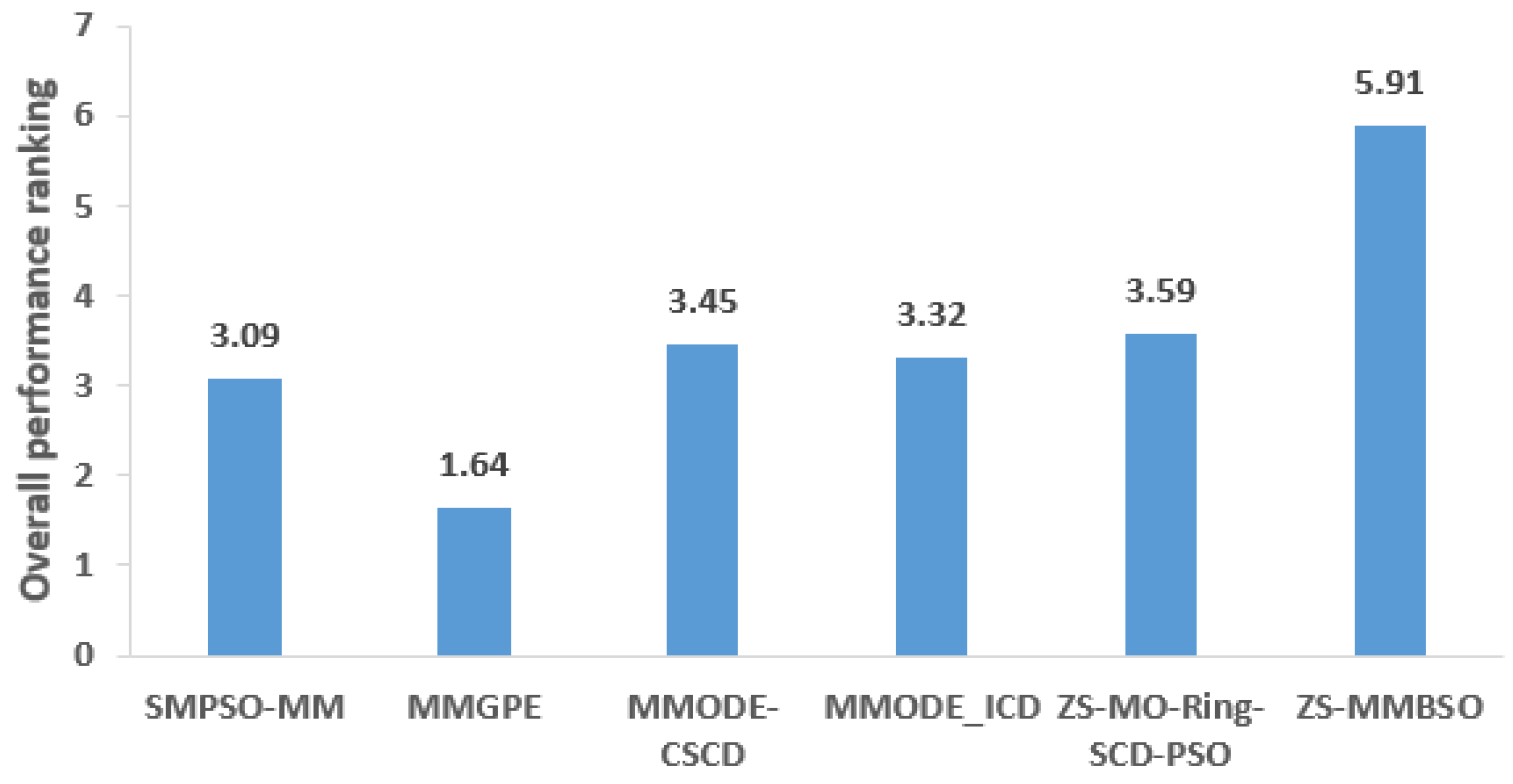
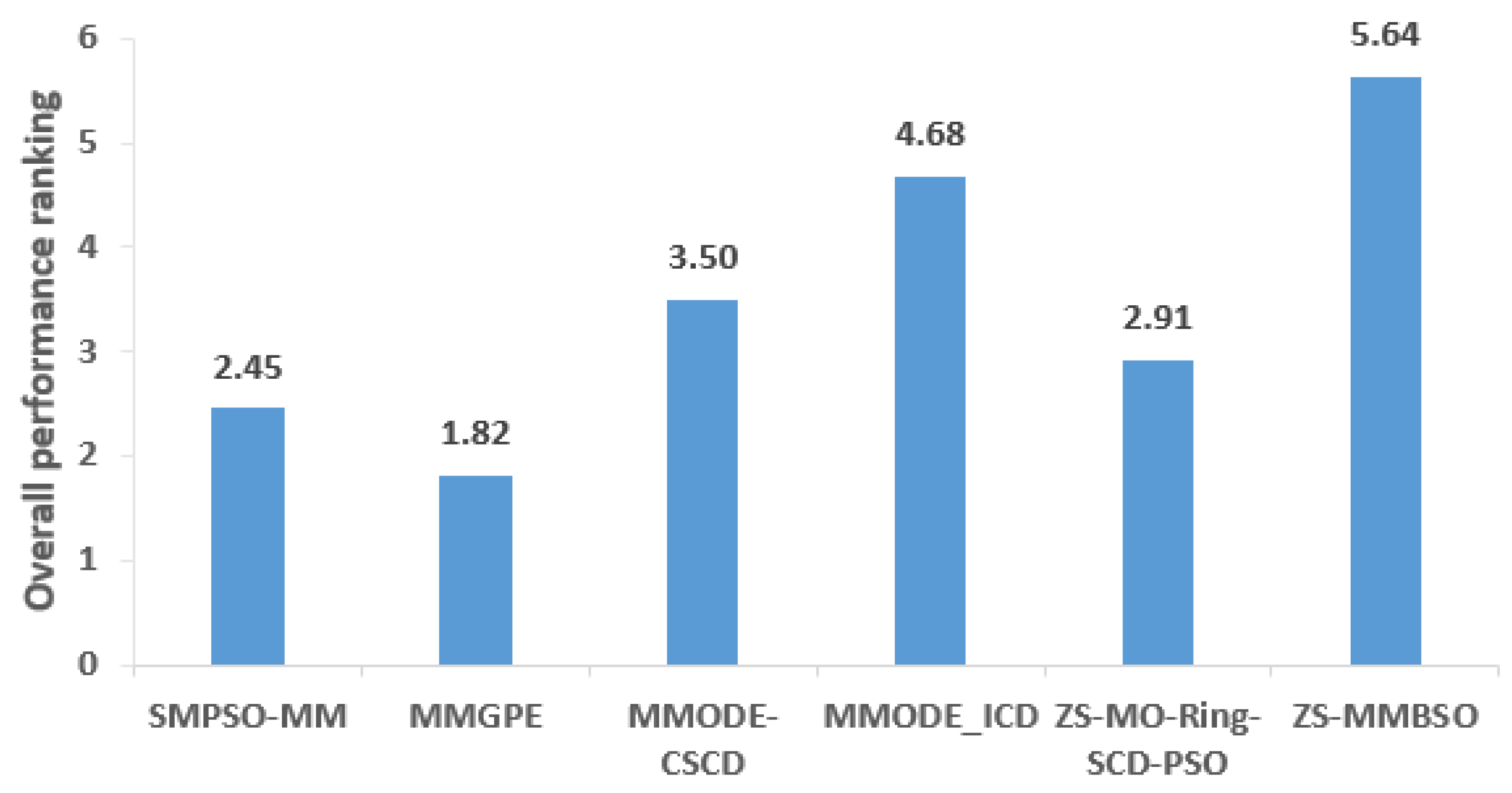
5.2. Comparison with Other Algorithms
5.3. Experimental Analysis
5.3.1. The Effectiveness of the ZS
5.3.2. The Effectiveness of the Novel Individual Generation Strategy
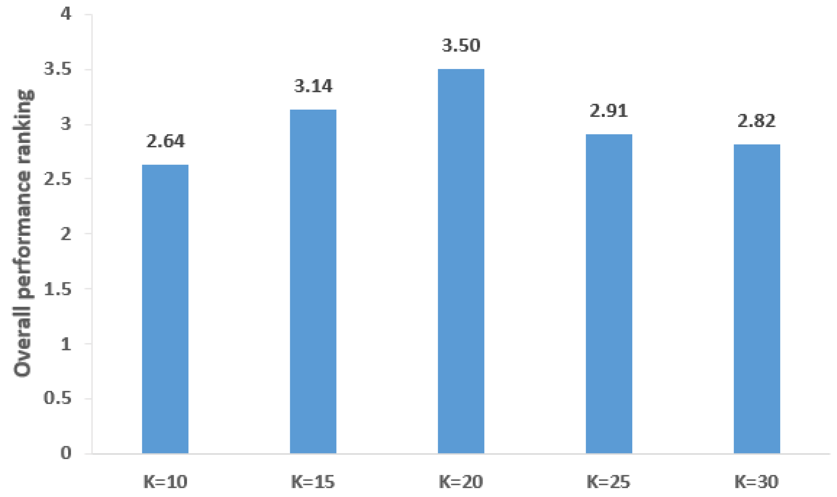
5.3.3. Impact of the Number of Clusters
6. Discussion
Author Contributions
Funding
Data Availability Statement
Conflicts of Interest
References
- Deb, K.; Pratap, A.; Agarwal, S.; Meyarivan, T. A fast and elitist multiobjective genetic algorithm: NSGA-II. IEEE Trans. Evol. Comput. 2002, 6, 182–197. [Google Scholar] [CrossRef]
- Hartikainen, M.; Miettinen, K.; Wiecek, M.M. PAINT: Pareto front interpolation for nonlinear multiobjective optimization. Comput. Optim. Appl. 2012, 52, 845–867. [Google Scholar] [CrossRef]
- Nedjah, N.; Mourelle, L.D. Evolutionary multi-objective optimisation: A survey. Int. J. Bio-Inspired Comput. 2015, 7, 1–25. [Google Scholar] [CrossRef]
- Liang, J.J.; Yue, C.T.; Qu, B.Y. Multimodal multi-objective optimization: A preliminary study. In Proceedings of the 2016 IEEE Congress on Evolutionary Computation (CEC), Vancouver, BC, Canada, 24–29 July 2016; pp. 2454–2461. [Google Scholar]
- Li, G.; Wang, W.; Chen, H.; You, W.; Wang, Y.; Jin, Y.; Zhang, W. A SHADE-based multimodal multi-objective evolutionary algorithm with fitness sharing. Appl. Intell. 2021, 51, 8720–8752. [Google Scholar] [CrossRef]
- Liang, J.; Qiao, K.; Yue, C.; Yu, K.; Qu, B.; Xu, R.; Li, Z.; Hu, Y. A clustering-based differential evolution algorithm for solving multimodal multi-objective optimization problems. Swarm Evol. Comput. 2021, 60, 100788. [Google Scholar] [CrossRef]
- Qu, B.; Li, C.; Liang, J.; Yan, L.; Yu, K.; Zhu, Y. A self-organized speciation based multi-objective particle swarm optimizer for multimodal multi-objective problems. Appl. Soft Comput. J. 2020, 86, 105886. [Google Scholar] [CrossRef]
- Wang, W.; Li, G.; Wang, Y.; Wu, F.; Zhang, W.; Li, L. Clearing-based multimodal multi-objective evolutionary optimization with layer-to-layer strategy. Swarm Evol. Comput. 2022, 68, 100976. [Google Scholar] [CrossRef]
- Li, W.; Zhang, T.; Wang, R.; Ishibuchi, H. Weighted Indicator-Based Evolutionary Algorithm for Multimodal Multiobjective Optimization. IEEE Trans. Evol. Comput. 2021, 25, 1064–1078. [Google Scholar] [CrossRef]
- Li, G.; Wang, W.; Zhang, W.; Wang, Z.; Tu, H.; You, W. Grid search based multi-population particle swarm optimization algorithm for multimodal multi-objective optimization. Swarm Evol. Comput. 2021, 62, 100843. [Google Scholar] [CrossRef]
- Qu, B.; Li, G.; Yan, L.; Liang, J.; Yue, C.; Yu, K.; Crisalle, O.D. A grid-guided particle swarm optimizer for multimodal multi-objective problems. Appl. Soft Comput. 2022, 117, 108381. [Google Scholar] [CrossRef]
- Liang, J.; Guo, Q.; Yue, C.; Qu, B.; Yu, K. A self-organizing multi-objective particle swarm optimization algorithm for multimodal multi-objective problems. In Proceedings of the 9th International Conference on Swarm Intelligence, ICSI 2018, Shanghai, China, 17–22 June 2018; Springer: Shanghai, China, 2018; pp. 550–560. [Google Scholar]
- Fan, Q.; Yan, X. Solving Multimodal Multiobjective Problems Through Zoning Search. IEEE Trans. Syst. Man Cybern. Syst. 2021, 51, 4836–4847. [Google Scholar] [CrossRef]
- Fan, Q.; Ersoy, O.K. Zoning Search With Adaptive Resource Allocating Method for Balanced and Imbalanced Multimodal Multi-Objective Optimization. IEEE/CAA J. Autom. Sin. 2021, 8, 1163–1176. [Google Scholar] [CrossRef]
- Guo, Y.-N.; Jiang, D.-Z.; Wang, R.-R.; Gong, D.-W. Structural design of heat exchanger plate with wide-channel based on multi-objective brain storm optimization. Kongzhi Yu Juece/Control Decis. 2022, 37, 2314–2322. [Google Scholar] [CrossRef]
- Hou, Y.; Wang, H.; Fu, Y.; Gao, K.; Zhang, H. Multi-Objective brain storm optimization for integrated scheduling of distributed flow shop and distribution with maximal processing quality and minimal total weighted earliness and tardiness. Comput. Ind. Eng. 2023, 179, 109217. [Google Scholar] [CrossRef]
- Cheng, S.; Chen, J.; Lei, X.; Shi, Y. Locating Multiple Optima via Brain Storm Optimization Algorithms. IEEE Access 2018, 6, 17039–17049. [Google Scholar] [CrossRef]
- Dai, Z.; Fang, W.; Li, Q.; Chen, W.-N. Modified Self-adaptive Brain Storm Optimization Algorithm for Multimodal Optimization. In Proceedings of the 14th International Conference on Bio-inspired Computing: Theories and Applications, BIC-TA 2019, Zhengzhou, China, 22–25 November 2019; Springer Science and Business Media Deutschland GmbH: Zhengzhou, China, 2020; pp. 384–397. [Google Scholar]
- Dai, Z.; Fang, W.; Tang, K.; Li, Q. An optima-identified framework with brain storm optimization for multimodal optimization problems. Swarm Evol. Comput. 2021, 62, 100827. [Google Scholar] [CrossRef]
- Guo, X.; Wu, Y.; Xie, L. Modified brain storm optimization algorithm for multimodal optimization. In Proceedings of the 5th International Conference on Advances in Swarm Intelligence, ICSI 2014, Hefei, China, 17–20 October 2014; pp. 340–351. [Google Scholar]
- Pourpanah, F.; Wang, R.; Wang, X.; Shi, Y.; Yazdani, D. mBSO: A Multi-Population Brain Storm Optimization for Multimodal Dynamic Optimization Problems. In Proceedings of the 2019 IEEE Symposium Series on Computational Intelligence (SSCI), Xiamen, China, 6–9 December 2019; pp. 673–679. [Google Scholar]
- Yue, C.; Qu, B.; Yu, K.; Liang, J.; Li, X. A novel scalable test problem suite for multimodal multiobjective optimization. Swarm Evol. Comput. 2019, 48, 62–71. [Google Scholar] [CrossRef]
- Yue, C.; Qu, B.; Liang, J. A Multiobjective Particle Swarm Optimizer Using Ring Topology for Solving Multimodal Multiobjective Problems. IEEE Trans. Evol. Comput. 2018, 22, 805–817. [Google Scholar] [CrossRef]
- Zitzler, E.; Thiele, L. Multiobjective evolutionary algorithms: A comparative case study and the strength Pareto approach. IEEE Trans. Evol. Comput. 1999, 3, 257–271. [Google Scholar] [CrossRef]
- Shi, Y. Brain storm optimization algorithm. In Proceedings of the Advances in Swarm Intelligence—Second International Conference, ICSI 2011, Chongqing, China, 12–15 June 2011; pp. 303–309. [Google Scholar]
- Deb, K.; Tiwari, S. Omni-optimizer: A procedure for single and multi-objective optimization. In Evolutionary Multi-Criterion Optimization; Coello, C.A.C., Aguirre, A.H., Zitzler, E., Eds.; Springer: Berlin/Heidelberg, Germany, 2005; Volume 3410, pp. 47–61. [Google Scholar]
- Zhang, J.-X.; Chu, X.-K.; Yang, F.; Qu, J.-F.; Wang, S.-W. Multimodal and multi-objective optimization algorithm based on two-stage search framework. Appl. Intell. 2022, 52, 12470–12496. [Google Scholar] [CrossRef]
- Li, G.; Zhou, T. A multi-objective particle swarm optimizer based on reference point for multimodal multi-objective optimization. Eng. Appl. Artif. Intell. 2022, 107, 104523. [Google Scholar] [CrossRef]
- Li, W.; Yao, X.; Zhang, T.; Wang, R.; Wang, L. Hierarchy Ranking Method for Multimodal Multiobjective Optimization With Local Pareto Fronts. IEEE Trans. Evol. Comput. 2023, 27, 98–110. [Google Scholar] [CrossRef]
- Hu, Z.B.; Zhou, T.; Su, Q.H.; Liu, M.F. A niching backtracking search algorithm with adaptive local search for multimodal multiobjective optimization. Swarm Evol. Comput. 2022, 69, 101031. [Google Scholar] [CrossRef]
- Hu, Y.; Wang, J.; Liang, J.; Wang, Y.L.; Ashraf, U.; Yue, C.T.; Yu, K.J. A two-archive model based evolutionary algorithm for multimodal multi-objective optimization problems. Appl. Soft Comput. 2022, 119, 108606. [Google Scholar] [CrossRef]
- Gao, W.; Xu, W.; Gong, M.; Yen, G.G. A decomposition-based evolutionary algorithm using an estimation strategy for multimodal multi-objective optimization. Inf. Sci. 2022, 606, 531–548. [Google Scholar] [CrossRef]
- Han, H.; Liu, Y.; Hou, Y.; Qiao, J. Multi-modal multi-objective particle swarm optimization with self-adjusting strategy. Inf. Sci. 2023, 629, 580–598. [Google Scholar] [CrossRef]
- Ming, F.; Gong, W.Y.; Wang, L.; Gao, L. Balancing Convergence and Diversity in Objective and Decision Spaces for Multimodal Multi-Objective Optimization. IEEE Trans. Emerg. Top. Comput. Intell. 2022, 7, 474–486. [Google Scholar] [CrossRef]
- Dang, Q.-L.; Xu, W.; Yuan, Y.-F. A Dynamic Resource Allocation Strategy with Reinforcement Learning for Multimodal Multi-objective Optimization. Mach. Intell. Res. 2022, 19, 138–152. [Google Scholar] [CrossRef]
- Ji, H.; Chen, S.; Fan, Q. Zoning Search and Transfer Learning-based Multimodal Multi-objective Evolutionary Algorithm. In Proceedings of the 2022 IEEE Congress on Evolutionary Computation, CEC 2022, Padua, Italy, 18–23 July 2022; Institute of Electrical and Electronics Engineers Inc.: Padua, Italy, 2022. [Google Scholar]
- Zhou, T.; Hu, Z.B.; Zhou, Q.; Yuan, S.X. A novel grey prediction evolution algorithm for multimodal multiobjective optimization. Eng. Appl. Artif. Intell. 2021, 100, 104173. [Google Scholar] [CrossRef]
- Yue, C.T.; Suganthan, P.N.; Liang, J.; Qu, B.Y.; Yu, K.J.; Zhu, Y.S.; Yan, L. Differential evolution using improved crowding distance for multimodal multiobjective optimization. Swarm Evol. Comput. 2021, 62, 100849. [Google Scholar] [CrossRef]
- Wilcoxon, F. Individual Comparisons by Ranking Methods. Biom. Bull. 1945, 1, 80–83. [Google Scholar] [CrossRef]
- Friedman, M. The Use of Ranks to Avoid the Assumption of Normality Implicit in the Analysis of Variance. J. Am. Stat. Assoc. 1937, 32, 675–701. [Google Scholar] [CrossRef]


| SMPSO_MM | MMGPE | MMODE_CSCD | MMODE_ICD | ZS-MO_Ring_PSO_SCD | ZS-MMBSO | ||||||
|---|---|---|---|---|---|---|---|---|---|---|---|
| MMF1 | 8.62 × 101 (3.67 × 100) | + | 6.72 × 101 (2.90 × 100) | + | 7.81 × 101 (3.90 × 100) | + | 7.12 × 101 (4.75 × 100) | + | 9.46 × 101 (4.63 × 100) | + | 1.99 × 10² (1.25 × 101) |
| MMF2 | 1.38 × 10² (2.15 × 101) | + | 1.32 × 10² (1.90 × 101) | + | 2.90 × 10² (4.52 × 101) | + | 2.11 × 10² (3.26 × 101) | + | 1.33 × 10² (1.78 × 101) | + | 1.22 × 10³ (2.21 × 10²) |
| MMF3 | 1.87 × 10² (1.42 × 101) | + | 1.86 × 10² (1.99 × 101) | + | 3.61 × 10² (4.39 × 101) | + | 2.58 × 10² (3.46 × 101) | + | 1.33 × 10² (2.09 × 101) | + | 9.28 × 10² (1.48 × 10²) |
| MMF4 | 1.39 × 10² (4.21 × 100) | + | 1.11 × 10² (4.40 × 100) | + | 1.49 × 10² (4.72 × 100) | + | 1.57 × 10² (6.50 × 100) | + | 1.90 × 10² (5.97 × 100) | + | 3.64 × 10² (1.10 × 101) |
| MMF5 | 3.97 × 101 (1.92 × 100) | + | 3.34 × 101 (1.21 × 100) | + | 3.85 × 101 (1.16 × 100) | + | 2.94 × 101 (1.49 × 100) | + | 4.86 × 101 (2.50 × 100) | + | 8.24 × 101 (5.29 × 100) |
| MMF6 | 4.23 × 101 (1.48 × 100) | + | 3.59 × 101 (9.56 × 10⁻¹) | + | 4.24 × 101 (1.16 × 100) | + | 3.37 × 101 (1.38 × 100) | + | 5.45 × 101 (2.95 × 100) | + | 8.04 × 101 (4.25 × 100) |
| MMF7 | 1.42 × 10² (4.94 × 100) | + | 1.10 × 10² (5.40 × 100) | + | 1.41 × 10² (5.95 × 100) | + | 1.60 × 10² (6.09 × 100) | + | 1.81 × 10² (9.23 × 100) | + | 2.86 × 10² (1.19 × 101) |
| MMF8 | 6.25 × 101 (3.47 × 100) | + | 4.26 × 101 (2.60 × 100) | + | 6.30 × 101 (2.28 × 100) | + | 2.66 × 101 (6.91 × 100) | + | 6.40 × 101 (2.73 × 100) | + | 1.67 × 10² (2.03 × 101) |
| MMF9 | 5.49 × 10² (2.10 × 101) | + | 3.89 × 10² (1.34 × 101) | + | 5.29 × 10² (1.85 × 101) | + | 8.15 × 10² (4.04 × 101) | + | 6.14 × 10² (2.04 × 101) | + | 1.53 × 10³ (5.89 × 101) |
| MMF10 | 2.55 × 10³ (1.89 × 10²) | + | 1.77 × 10² (3.15 × 101) | + | 1.98 × 10³ (1.80 × 10²) | + | 1.41 × 10³ (4.65 × 10²) | + | 1.37 × 10² (1.59 × 101) | + | 3.16 × 10³ (2.91 × 101) |
| MMF11 | 7.63 × 10² (4.11 × 101) | + | 4.92 × 10² (1.70 × 101) | + | 6.52 × 10² (4.16 × 101) | + | 7.22 × 10² (1.74 × 101) | + | 6.17 × 10² (2.30 × 101) | + | 1.15 × 10³ (4.77 × 101) |
| MMF12 | 1.29 × 10³ (9.39 × 101) | + | 6.17 × 10² (5.65 × 101) | + | 1.46 × 10³ (5.47 × 101) | + | 1.01 × 10³ (2.84 × 101) | + | 8.68 × 10² (4.59 × 101) | + | 1.83 × 10³ (6.82 × 101) |
| MMF13 | 6.67 × 101 (2.22 × 100) | + | 5.06 × 101 (9.91 × 10⁻¹) | + | 7.12 × 101 (1.29 × 100) | + | 6.50 × 101 (1.87 × 100) | + | 5.74 × 101 (1.75 × 100) | + | 7.76 × 101 (3.84 × 100) |
| MMF14 | 2.98 × 101 (4.26 × 10⁻¹) | + | 3.00 × 101 (4.25 × 10⁻¹) | + | 3.15 × 101 (8.69 × 10⁻¹) | + | 4.00 × 101 (5.84 × 10⁻¹) | + | 5.32 × 101 (5.36 × 10⁻¹) | + | 5.77 × 101 (8.39 × 10⁻¹) |
| MMF15 | 3.95 × 101 (9.86 × 10⁻¹) | + | 3.81 × 101 (1.34 × 100) | + | 3.98 × 101 (1.15 × 100) | + | 5.49 × 101 (1.57 × 100) | + | 6.54 × 101 (1.20 × 100) | + | 7.76 × 101 (1.27 × 100) |
| MMF1_z | 1.19 × 10² (5.12 × 100) | + | 9.01 × 101 (2.91 × 100) | + | 1.13 × 10² (5.02 × 100) | + | 5.52 × 101 (4.38 × 100) | + | 1.27 × 10² (4.47 × 100) | + | 2.70 × 10² (1.90 × 101) |
| MMF1_e | 6.77 × 100 (8.28 × 10⁻¹) | + | 5.86 × 100 (6.15 × 10⁻¹) | + | 6.77 × 100 (6.20 × 10⁻¹) | + | 1.24 × 100 (5.20 × 10⁻¹) | + | 4.63 × 100 (1.11 × 100) | + | 8.23 × 100 (6.20 × 10⁻¹) |
| MMF14_a | 2.66 × 101 (5.83 × 10⁻¹) | + | 2.66 × 101 (5.65 × 10⁻¹) | + | 2.62 × 101 (4.20 × 10⁻¹) | + | 2.90 × 101 (4.97 × 10⁻¹) | + | 4.82 × 101 (4.79 × 10⁻¹) | + | 4.94 × 101 (9.01 × 10⁻¹) |
| MMF15_a | 3.59 × 101 (5.74 × 10⁻¹) | + | 3.61 × 101 (6.76 × 10⁻¹) | + | 3.47 × 101 (1.12 × 100) | + | 4.39 × 101 (9.36 × 10⁻¹) | + | 6.07 × 101 (9.83 × 10⁻¹) | + | 6.80 × 101 (1.40 × 100) |
| SYM_PART simple | 3.15 × 101 (2.52 × 100) | + | 1.23 × 101 (1.27 × 100) | + | 6.17 × 101 (1.68 × 100) | + | 1.03 × 10² (4.45 × 100) | - | 2.16 × 101 (9.85 × 10⁻¹) | + | 9.22 × 101 (9.45 × 100) |
| SYM_PART rotated | 1.67 × 101 (1.08 × 100) | + | 2.40 × 101 (1.55 × 100) | + | 6.27 × 101 (2.57 × 100) | + | 5.98 × 101 (3.06 × 100) | + | 2.03 × 101 (1.00 × 100) | + | 1.25 × 10² (1.45 × 101) |
| Omni_test | 7.64 × 100 (1.50 × 100) | + | 5.10 × 101 (1.05 × 100) | + | 8.16 × 100 (3.18 × 100) | + | 5.46 × 101 (1.97 × 100) | - | 9.34 × 100 (1.29 × 100) | + | 3.04 × 101 (4.22 × 100) |
| + | 22 | 22 | 22 | 20 | 22 | ||||||
| = | 0 | 0 | 0 | 0 | 0 | ||||||
| - | 0 | 0 | 0 | 2 | 0 |
| SMPSO_MM | MMGPE | MMODE_CSCD | MMODE_ICD | ZS-MO_Ring_PSO_SCD | ZS-MMBSO | ||||||
|---|---|---|---|---|---|---|---|---|---|---|---|
| MMF1 | 8.76 × 10⁻¹ (5.23 × 10⁻⁵) | + | 8.75 × 10⁻¹ (6.88 × 10⁻⁵) | + | 8.76 × 10⁻¹ (3.64 × 10⁻⁵) | + | 8.76 × 10⁻¹ (1.13 × 10⁻⁵) | + | 8.76 × 10⁻¹ (6.69 × 10⁻⁵) | + | 8.76 × 10⁻¹ (3.63 × 10⁻⁵) |
| MMF2 | 8.71 × 10⁻¹ (4.56 × 10⁻⁴) | + | 8.71 × 10⁻¹ (5.12 × 10⁻⁴) | + | 8.74 × 10⁻¹ (1.89 × 10⁻⁴) | + | 8.74 × 10⁻¹ (5.64 × 10⁻⁴) | + | 8.70 × 10⁻¹ (7.74 × 10⁻⁴) | + | 8.76 × 10⁻¹ (3.54 × 10⁻⁴) |
| MMF3 | 8.72 × 10⁻¹ (4.01 × 10⁻⁴) | + | 8.72 × 10⁻¹ (3.94 × 10⁻⁴) | + | 8.74 × 10⁻¹ (9.24 × 10⁻⁵) | + | 8.75 × 10⁻¹ (2.50 × 10⁻⁴) | + | 8.70 × 10⁻¹ (9.45 × 10⁻⁴) | + | 8.76 × 10⁻¹ (2.50 × 10⁻⁴) |
| MMF4 | 5.42 × 10⁻¹ (8.93 × 10⁻⁵) | + | 5.42 × 10⁻¹ (7.81 × 10⁻⁵) | + | 5.42 × 10⁻¹ (8.17 × 10⁻⁵) | + | 5.43 × 10⁻¹ (2.04 × 10⁻⁵) | + | 5.42 × 10⁻¹ (1.42 × 10⁻⁴) | + | 5.43 × 10⁻¹ (6.03 × 10⁻⁵) |
| MMF5 | 8.76 × 10⁻¹ (3.66 × 10⁻⁵) | + | 8.75 × 10⁻¹ (5.18 × 10⁻⁵) | + | 8.76 × 10⁻¹ (4.94 × 10⁻⁵) | + | 8.76 × 10⁻¹ (1.92 × 10⁻⁵) | + | 8.76 × 10⁻¹ (6.58 × 10⁻⁵) | + | 8.76 × 10⁻¹ (5.03 × 10⁻⁵) |
| MMF6 | 8.76 × 10⁻¹ (5.06 × 10⁻⁵) | + | 8.75 × 10⁻¹ (8.26 × 10⁻⁵) | + | 8.76 × 10⁻¹ (4.19 × 10⁻⁵) | + | 8.76 × 10⁻¹ (3.96 × 10⁻⁵) | + | 8.76 × 10⁻¹ (6.01 × 10⁻⁵) | + | 8.76 × 10⁻¹ (7.58 × 10⁻⁵) |
| MMF7 | 8.76 × 10⁻¹ (2.79 × 10⁻⁵) | + | 8.75 × 10⁻¹ (9.18 × 10⁻⁵) | + | 8.76 × 10⁻¹ (2.53 × 10⁻⁵) | + | 8.76 × 10⁻¹ (2.03 × 10⁻⁵) | + | 8.76 × 10⁻¹ (3.04 × 10⁻⁵) | + | 8.76 × 10⁻¹ (2.34 × 10⁻⁵) |
| MMF8 | 4.23 × 10⁻¹ (1.18 × 10⁻⁴) | + | 4.23 × 10⁻¹ (1.73 × 10⁻⁴) | + | 4.24 × 10⁻¹ (1.17 × 10⁻⁴) | + | 4.24 × 10⁻¹ (1.11 × 10⁻⁴) | + | 4.23 × 10⁻¹ (2.58 × 10⁻⁴) | + | 4.24 × 10⁻¹ (3.51 × 10⁻⁴) |
| MMF9 | 9.70 × 100 (3.48 × 10⁻⁴) | + | 9.70 × 100 (5.97 × 10⁻⁴) | + | 9.70 × 100 (1.35 × 10⁻⁴) | + | 9.71 × 100 (3.01 × 10⁻⁴) | + | 9.71 × 100 (2.58 × 10⁻⁴) | + | 9.71 × 100 (3.15 × 10⁻⁴) |
| MMF10 | 1.29 × 101 (9.73 × 10⁻⁴) | = | 1.43 × 100 (2.01 × 10⁻²) | + | 1.29 × 101 (1.62 × 10⁻⁴) | - | 1.28 × 101 (9.44 × 10⁻²) | = | 1.28 × 101 (1.09 × 10⁻²) | + | 1.29 × 101 (4.51 × 10⁻³) |
| MMF11 | 1.45 × 101 (4.96 × 10⁻⁴) | + | 1.45 × 101 (5.56 × 10⁻⁴) | + | 1.45 × 101 (2.30 × 10⁻⁴) | + | 1.45 × 101 (2.76 × 10⁻⁴) | + | 1.45 × 101 (4.99 × 10⁻⁴) | + | 1.45 × 101 (4.48 × 10⁻⁴) |
| MMF12 | 1.57 × 100 (1.32 × 10⁻⁴) | + | 1.57 × 100 (2.98 × 10⁻⁴) | + | 1.57 × 100 (6.55 × 10⁻⁶) | = | 1.57 × 100 (4.87 × 10⁻⁵) | = | 1.57 × 100 (6.83 × 10⁻⁴) | + | 1.57 × 100 (1.07 × 10⁻⁴) |
| MMF13 | 1.85 × 101 (1.10 × 10⁻³) | + | 1.84 × 101 (2.30 × 10⁻³) | + | 1.85 × 101 (1.82 × 10⁻⁴) | + | 1.85 × 101 (6.12 × 10⁻⁴) | + | 1.84 × 101 (1.90 × 10⁻³) | + | 1.85 × 101 (6.77 × 10⁻⁴) |
| MMF14 | 2.95 × 100 (9.22 × 10⁻²) | + | 3.02 × 100 (3.85 × 10⁻²) | + | 2.88 × 100 (1.31 × 10⁻¹) | + | 3.16 × 100 (5.40 × 10⁻²) | = | 3.05 × 100 (2.12 × 10⁻¹) | + | 3.15 × 100 (1.35 × 10⁻¹) |
| MMF15 | 4.33 × 100 (8.93 × 10⁻²) | + | 4.36 × 100 (3.04 × 10⁻²) | + | 4.13 × 100 (1.10 × 10⁻¹) | + | 4.52 × 100 (5.16 × 10⁻²) | = | 4.40 × 100 (1.14 × 10⁻¹) | + | 4.48 × 100 (1.13 × 10⁻¹) |
| MMF1_z | 8.76 × 10⁻¹ (3.70 × 10⁻⁵) | + | 8.75 × 10⁻¹ (7.85 × 10⁻⁵) | + | 8.76 × 10⁻¹ (5.82 × 10⁻⁵) | + | 8.76 × 10⁻¹ (2.63 × 10⁻⁵) | + | 8.76 × 10⁻¹ (7.05 × 10⁻⁵) | + | 8.76 × 10⁻¹ (1.86 × 10⁻⁵) |
| MMF1_e | 8.73 × 10⁻¹ (8.39 × 10⁻⁴) | + | 8.71 × 10⁻¹ (9.87 × 10⁻⁴) | + | 8.64 × 10⁻¹ (5.10 × 10⁻³) | + | 8.75 × 10⁻¹ (2.49 × 10⁻⁴) | - | 8.70 × 10⁻¹ (9.00 × 10⁻⁴) | + | 8.74 × 10⁻¹ (8.20 × 10⁻⁴) |
| MMF14_a | 3.03 × 100 (6.85 × 10⁻²) | + | 3.05 × 100 (6.18 × 10⁻²) | + | 2.88 × 100 (1.72 × 10⁻¹) | + | 3.12 × 100 (4.22 × 10⁻²) | + | 3.07 × 100 (1.49 × 10⁻¹) | + | 3.23 × 100 (2.01 × 10⁻¹) |
| MMF15_a | 4.27 × 100 (1.11 × 10⁻¹) | + | 4.42 × 100 (4.35 × 10⁻²) | + | 4.16 × 100 (1.47 × 10⁻¹) | + | 4.45 × 100 (4.24 × 10⁻²) | + | 4.47 × 100 (7.66 × 10⁻²) | = | 4.49 × 100 (7.99 × 10⁻²) |
| SYM_PART simple | 1.67 × 101 (1.20 × 10⁻³) | + | 1.66 × 101 (6.62 × 10⁻³) | + | 1.67 × 101 (1.14 × 10⁻⁴) | + | 1.67 × 101 (1.40 × 10⁻⁴) | + | 1.67 × 101 (1.50 × 10⁻³) | + | 1.67 × 101 (3.44 × 10⁻⁵) |
| SYM_PART rotated | 1.66 × 101 (2.20 × 10⁻³) | + | 1.67 × 101 (2.15 × 10⁻³) | + | 1.67 × 101 (2.06 × 10⁻⁴) | + | 1.67 × 101 (1.38 × 10⁻⁴) | + | 1.67 × 101 (2.00 × 10⁻³) | + | 1.67 × 101 (6.33 × 10⁻⁵) |
| Omni_test | 5.27 × 101 (1.00 × 10⁻²) | + | 5.27 × 101 (1.47 × 10⁻²) | + | 5.28 × 101 (6.06 × 10⁻³) | + | 5.28 × 101 (1.72 × 10⁻³) | + | 5.27 × 101 (1.28 × 10⁻²) | + | 5.28 × 101 (1.26 × 10⁻³) |
| + | 21 | 22 | 20 | 17 | 21 | ||||||
| = | 1 | 0 | 1 | 4 | 1 | ||||||
| - | 0 | 0 | 1 | 1 | 0 |
| ZS-MMBSO_1 | ZS-MMBSO | ||
|---|---|---|---|
| MMF1 | 8.38 × 101 (2.95 × 100) | + | 1.99 × 10² (1.25 × 101) |
| MMF2 | 3.90 × 10² (9.44 × 101) | + | 1.22 × 10³ (2.21 × 10²) |
| MMF3 | 2.94 × 10² (7.88 × 101) | + | 9.28 × 10² (1.48 × 10²) |
| MMF4 | 8.42 × 101 (1.25 × 101) | + | 3.64 × 10² (1.10 × 101) |
| MMF5 | 3.36 × 101 (2.08 × 100) | + | 8.24 × 101 (5.29 × 100) |
| MMF6 | 3.75 × 101 (1.65 × 100) | + | 8.04 × 101 (4.25 × 100) |
| MMF7 | 1.39 × 10² (6.75 × 100) | + | 2.86 × 10² (1.19 × 100) |
| MMF8 | 2.66 × 101 (7.53 × 100) | + | 1.67 × 10² (2.03 × 101) |
| MMF9 | 5.30 × 10² (1.02 × 10²) | + | 1.53 × 10³ (5.89 × 101) |
| MMF10 | 2.34 × 10³ (1.53 × 101) | + | 3.16 × 10³ (2.91 × 101) |
| MMF11 | 7.98 × 10² (6.19 × 101) | + | 1.15 × 10³ (4.77 × 101) |
| MMF12 | 1.33 × 10³ (2.23 × 101) | + | 1.83 × 10³ (6.82 × 101) |
| MMF13 | 4.36 × 101 (9.91 × 100) | + | 7.76 × 101 (3.84 × 100) |
| MMF14 | 2.68 × 101 (1.92 × 100) | + | 5.77 × 101 (8.39 × 10⁻¹) |
| MMF15 | 3.90 × 101 (1.20 × 100) | + | 7.76 × 101 (1.27 × 100) |
| MMF1_z | 9.62 × 101 (5.76 × 100) | + | 2.70 × 10² (1.90 × 101) |
| MMF1_e | 5.37 × 100 (1.59 × 100) | + | 8.23 × 100 (6.20 × 10⁻¹) |
| MMF14_a | 2.18 × 101 (1.23 × 100) | + | 4.94 × 101 (9.01 × 10⁻¹) |
| MMF15_a | 3.07 × 101 (1.96 × 100) | + | 6.80 × 101 (1.40 × 100) |
| SYM_PART simple | 3.70 × 101 (1.25 × 101) | + | 9.22 × 101 (9.45 × 100) |
| SYM_PART rotated | 6.30 × 101 (8.06 × 100) | + | 1.25 × 10² (1.45 × 101) |
| Omni_test | 1.98 × 100 (5.10 × 10⁻¹) | + | 3.04 × 101 (4.22 × 100) |
| + | 22 | ||
| = | 0 | ||
| - | 0 |
| ZS-MMBSO_2 | ZS-MMBSO | ||
|---|---|---|---|
| MMF1 | 1.24 × 10² (4.88 × 100) | + | 1.99 × 10² (1.25 × 101) |
| MMF2 | 1.69 × 10² (9.98 × 100) | + | 1.22 × 10³ (2.21 × 10²) |
| MMF3 | 1.74 × 10² (1.34 × 101) | + | 9.28 × 10² (1.48 × 10²) |
| MMF4 | 2.64 × 10² (9.27 × 100) | + | 3.64 × 10² (1.10 × 101) |
| MMF5 | 6.17 × 101 (2.54 × 100) | + | 8.24 × 101 (5.29 × 100) |
| MMF6 | 7.52 × 101 (3.69 × 100) | + | 8.04 × 101 (4.25 × 100) |
| MMF7 | 2.54 × 10² (1.13 × 101) | + | 2.86 × 10² (1.19 × 100) |
| MMF8 | 1.21 × 10² (6.61 × 100) | + | 1.67 × 10² (2.03 × 101) |
| MMF9 | 7.15 × 10² (1.94 × 101) | + | 1.53 × 10³ (5.89 × 101) |
| MMF10 | 2.30 × 10² (2.85 × 101) | + | 3.16 × 10³ (2.91 × 101) |
| MMF11 | 7.14 × 10² (2.91 × 101) | + | 1.15 × 10³ (4.77 × 101) |
| MMF12 | 7.08 × 10² (4.92 × 101) | + | 1.83 × 10³ (6.82 × 101) |
| MMF13 | 6.23 × 101 (2.15 × 100) | + | 7.76 × 101 (3.84 × 100) |
| MMF14 | 5.77 × 101 (6.05 × 10⁻¹) | = | 5.77 × 101 (8.39 × 10⁻¹) |
| MMF15 | 7.41 × 101 (9.13 × 10⁻¹) | + | 7.76 × 101 (1.27 × 100) |
| MMF1_z | 1.63 × 10² (5.58 × 100) | + | 2.70 × 10² (1.90 × 101) |
| MMF1_e | 6.76 × 100 (7.15 × 10⁻¹) | + | 8.23 × 100 (6.20 × 10⁻¹) |
| MMF14_a | 5.11 × 101 (5.41 × 10⁻¹) | - | 4.94 × 101 (9.01 × 10⁻¹) |
| MMF15_a | 6.68 × 101 (8.58 × 10⁻¹) | + | 6.80 × 101 (1.40 × 100) |
| SYM_PART simple | 1.00 × 10² (4.37 × 100) | - | 9.22 × 101 (9.45 × 100) |
| SYM_PART rotated | 1.01 × 10² (4.36 × 100) | + | 1.25 × 10² (1.45 × 101) |
| Omni_test | 1.99 × 101 (1.62 × 100) | + | 3.04 × 101 (4.22 × 100) |
| + | 19 | ||
| = | 1 | ||
| - | 2 |
| 10 | 15 | 20 | 25 | 30 | |
|---|---|---|---|---|---|
| MMF1 | 1.66 × 10² (9.23 × 100) | 1.76 × 10² (9.95 × 10⁻¹) | 1.99 × 10² (1.25 × 101) | 2.07 × 10² (1.01 × 101) | 2.16 × 10² (1.21 × 101) |
| MMF2 | 1.04 × 10³ (1.42 × 10²) | 1.16 × 10³ (1.24 × 10²) | 1.22 × 10³ (2.21 × 10²) | 1.31 × 10³ (1.77 × 10²) | 1.25 × 10³ (1.96 × 10²) |
| MMF3 | 7.97 × 10² (1.64 × 10²) | 9.37 × 10² (1.20 × 10²) | 9.28 × 10² (1.48 × 10²) | 9.16 × 10² (2.04 × 10²) | 9.21 × 10² (1.54 × 10²) |
| MMF4 | 3.52 × 10² (8.24 × 100) | 3.59 × 10² (9.81 × 100) | 3.64 × 10² (1.10 × 101) | 3.57 × 10² (1.27 × 101) | 3.56 × 10² (1.23 × 101) |
| MMF5 | 7.45 × 101 (4.39 × 100) | 7.89 × 101 (4.28 × 100) | 8.24 × 101 (5.29 × 100) | 8.32 × 101 (3.96 × 100) | 8.75 × 101 (4.28 × 100) |
| MMF6 | 7.68 × 101 (3.48 × 100) | 7.86 × 101 (2.60 × 100) | 8.04 × 101 (4.25 × 100) | 8.29 × 101 (2.99 × 100) | 8.36 × 101 (3.64 × 100) |
| MMF7 | 2.70 × 10² (1.20 × 101) | 2.75 × 10² (1.19 × 101) | 2.86 × 10² (1.19 × 101) | 2.84 × 10² (1.26 × 101) | 2.94 × 10² (1.04 × 101) |
| MMF8 | 1.66 × 10² (2.11 × 101) | 1.67 × 10² (2.44 × 101) | 1.67 × 10² (2.03 × 101) | 1.68 × 10² (1.91 × 101) | 1.65 × 10² (2.12 × 101) |
| MMF9 | 1.53 × 10³ (6.41 × 101) | 1.53 × 10³ (6.10 × 101) | 1.53 × 10³ (5.89 × 101) | 1.52 × 10³ (5.70 × 101) | 1.52 × 10³ (5.47 × 101) |
| MMF10 | 2.97 × 10³ (6.61 × 10²) | 3.08 × 10³ (7.65 × 10²) | 3.16 × 10³ (2.91 × 101) | 2.84 × 10³ (7.06 × 10²) | 2.65 × 10³ (7.47 × 10²) |
| MMF11 | 1.17 × 10³ (5.05 × 101) | 1.15 × 10³ (4.82 × 101) | 1.15 × 10³ (4.77 × 101) | 1.15 × 10³ (5.45 × 101) | 1.15 × 10³ (4.33 × 101) |
| MMF12 | 1.83 × 10³ (7.57 × 101) | 1.84 × 10³ (7.17 × 101) | 1.83 × 10³ (6.82 × 101) | 1.83 × 10³ (6.19 × 101) | 1.76 × 10³ (8.67 × 101) |
| MMF13 | 7.42 × 101 (6.60 × 100) | 7.59 × 101 (6.25 × 100) | 7.76 × 101 (3.84 × 100) | 7.73 × 101 (4.06 × 100) | 7.66 × 101 (3.86 × 100) |
| MMF14 | 5.86 × 101 (8.46 × 10⁻¹) | 5.80 × 101(5.65 × 10⁻¹) | 5.77 × 101 (8.39 × 10⁻¹) | 5.75 × 101 (8.70 × 10⁻¹) | 5.68 × 101 (8.82 × 10⁻¹) |
| MMF15 | 7.80 × 101 (1.06 × 100) | 7.77 × 101 (1.16 × 100) | 7.76 × 101 (1.27 × 100) | 7.63 × 101 (1.31 × 100) | 7.62 × 101 (1.22 × 100) |
| MMF1_z | 2.24 × 10² (2.22 × 101) | 2.54 × 10² (1.71 × 101) | 2.70 × 10² (1.90 × 101) | 2.91 × 10² (1.74 × 101) | 3.00 × 10² (1.66 × 101) |
| MMF1_e | 7.17 × 100 (9.16 × 10⁻¹) | 8.24 × 100 (7.13 × 10⁻¹) | 8.23 × 100 (6.20 × 10⁻¹) | 8.23 × 100 (1.03 × 100) | 8.59 × 100 (9.81 × 10⁻¹) |
| MMF14_a | 5.02 × 101 (7.29 × 10⁻¹) | 4.96 × 101 (5.89 × 10⁻¹) | 4.94 × 101 (9.01 × 10⁻¹) | 4.86 × 101 (1.02 × 100) | 4.84 × 101 (6.84 × 10⁻¹) |
| MMF15_a | 6.93 × 101 (1.33 × 100) | 6.85 × 101 (1.60 × 100) | 6.80 × 101 (1.40 × 100) | 6.72 × 101 (1.56 × 100) | 6.67 × 101 (1.24 × 100) |
| SYM_PART simple | 1.01 × 10² (1.10 × 101) | 9.60 × 101 (1.01 × 101) | 9.22 × 101 (9.45 × 100) | 9.20 × 101 (9.48 × 100) | 8.50 × 101 (9.85 × 100) |
| SYM_PART rotated | 1.24 × 10² (1.51 × 101) | 1.21 × 10² (1.90 × 101) | 1.25 × 10² (1.45 × 101) | 1.22 × 10² (1.68 × 101) | 1.26 × 10² (1.12 × 101) |
| Omni_test | 1.38 × 101 (6.81 × 100) | 3.11 × 101 (8.24 × 100) | 3.04 × 101 (4.22 × 100) | 3.10 × 101 (3.01 × 100) | 3.01 × 101 (5.28 × 100) |
Disclaimer/Publisher’s Note: The statements, opinions and data contained in all publications are solely those of the individual author(s) and contributor(s) and not of MDPI and/or the editor(s). MDPI and/or the editor(s) disclaim responsibility for any injury to people or property resulting from any ideas, methods, instructions or products referred to in the content. |
© 2023 by the authors. Licensee MDPI, Basel, Switzerland. This article is an open access article distributed under the terms and conditions of the Creative Commons Attribution (CC BY) license (https://creativecommons.org/licenses/by/4.0/).
Share and Cite
Fan, J.; Huang, W.; Jiang, Q.; Fan, Q. A Zoning Search-Based Multimodal Multi-Objective Brain Storm Optimization Algorithm for Multimodal Multi-Objective Optimization. Algorithms 2023, 16, 350. https://doi.org/10.3390/a16070350
Fan J, Huang W, Jiang Q, Fan Q. A Zoning Search-Based Multimodal Multi-Objective Brain Storm Optimization Algorithm for Multimodal Multi-Objective Optimization. Algorithms. 2023; 16(7):350. https://doi.org/10.3390/a16070350
Chicago/Turabian StyleFan, Jiajia, Wentao Huang, Qingchao Jiang, and Qinqin Fan. 2023. "A Zoning Search-Based Multimodal Multi-Objective Brain Storm Optimization Algorithm for Multimodal Multi-Objective Optimization" Algorithms 16, no. 7: 350. https://doi.org/10.3390/a16070350
APA StyleFan, J., Huang, W., Jiang, Q., & Fan, Q. (2023). A Zoning Search-Based Multimodal Multi-Objective Brain Storm Optimization Algorithm for Multimodal Multi-Objective Optimization. Algorithms, 16(7), 350. https://doi.org/10.3390/a16070350