2. Generating Loop Patterns with a Genetic Algorithm
First, we will show how 2D patterns can be generated by a GA using a set of local matching patterns (tiles). Then, a tile set is designed that can generate loop patterns.
We aim at binary patterns S of size , where the elements , and the coordinates …}. We may call the elements also “cells” as we will later deal with cellular automata cells and patterns of them. We will use also the term “field” or “space” for an array of cells.
2.1. Tile
A tile L is a pattern of elements where . We call the elements “pixels” in order to distinguish them from cells. The symbol “-” represents a null, a pixel that is not part of a tile. A non-null pixel 0/1 is also called a valid pixel. We want to use only tiles that are much smaller (or smaller for small fields) than the size of the whole field. The reason is that we do want to allow that a few large tiles of size and/or may simply cover the whole global space. Then, a trivial solution could be that just one tile is equal to the aimed pattern. In fact, we want to restrict the size of the tiles, and , where are the boundaries of a tile, and where . Here, we want to solve the problem with small tiles of size . The coordinates within a tile L are locally defined separately for each tile where the origin is assigned to the central pixel of a tile.
Remark. It would be possible to define a tile as a set of pixels where are the coordinates and are the states of a pixel. In addition, the name of the tile and the anchor’s position have to be related.
2.2. Overlapping Tiles
Now, we search for global patterns that can be tiled by tiles from a set of tiles
….} that may overlap. Two tiles
,
,
overlap if they are overlaid (shifted relative to each other) and all overlaid non-null pixels have the same value. The result of overlaying a pixel
from
with a pixel
from
is summarized in
Table 1.
It is possible that tiles overlap. In this case, there exists pairwise an overlap and the resulting overlap forms a compound tile consisting of k sub-tiles. In terms of particle systems, we may associate a basic particle with a (basic) tile, and a compound/complex particle with a compound tile.
Two tiles may also overlap (by inclusion) if is smaller than but compatible with it ( has the same pixel structure as except that some of the valid –pixels are null in ). Overlap by inclusion is symmetric.
We define a field of cells as fully covered if all cells are covered by tiles (the number is not restricted) taken from the given set of tiles, and tiles are allowed to overlap as explained already. In order to cover the field, not only the basic tiles but also compound tiles can be used. Due to a not properly defined set of tiles, it may happen that a given field cannot totally be covered by valid pixels. Then, the field is partially (not fully) covered because it contains uncovered cells (null pixels, gaps, wholes, spaces). Nevertheless, partially covered fields may be of interest as patterns too.
2.3. Genetic Algorithm
In the first stage, we use a GA to find optimal patterns with respect to a global fitness function and defined by tiles. The main purpose here is to validate that a certain set of designed tiles define the patterns that are aimed at the user and that can be used later by the CA rule in the second stage.
The algorithm used is given in Algorithm 1. A possible solution (an individual) is a tuple (Pattern, Fitness). An array/list of M solutions is the data and output that is manipulated by the algorithm. (1) The pattern list is initialized randomly. (2) The while loop is repeated until a termination condition becomes true, i.e., the number of iterations reaches a certain limit, and / or another global condition, like a certain fitness level or certain pattern features. (3) In each block, better solutions are searched for. For each current existing individual (tentative solution), an offspring (a new individual) is generated by crossover and mutation. The current individual is replaced by the offspring if it has higher fitness. (4) A mate is selected at random from the list. (5) A new offspring pattern is computed by crossing over with , and then applying a mutation. (6) The fitness of the offspring pattern is computed and stored within the offspring. (7) The offspring replaces the current individual if its fitness is higher. (8) The list of solutions is sorted for output.
The fitness function computes the number of tile matches that occurs within a pattern. At every site of the pattern, all tiles from the given set are tested if they match locally, i.e., test if all tile pixels (aligned to the tile’s anchor/center) are equal to the pattern values in the local neighborhood. A null tile pixel (do not care) excludes the testing of the corresponding pattern value.
The used GA is a simple form using the classical GA algorithm basics. The goal was to generate optimal patterns in a simple way and not to optimize the algorithm itself, which is a topic for further research. Only one list of individuals is used and not two (old and new generation).
| Algorithm 1: Generating a Binary Pattern with a Genetic Algorithm |
| Types: Pattern = array [0 … n1 − 1, 0 … n2 − 1] of {0,1} |
| Solution = (Pattern, Fitness) |
| Data and Output: S is an array [1 … M] of Solution |
| Temporary: Offspring is a Solution |
| (1) S.Pattern ← RandomPatterns |
| (2) while not TerminationCondition |
| (3) foreach Si in S |
| (4) Select randomly a Mate Sj |
| (5) Offspring.Pattern = Mutate (Crossover (Si, Sj)) |
| (6) Offspring.Fitness ← fitness (Offspring.Pattern) |
| (7) if Offspring.Pattern ∉ S.Pattern and Offspring.Fitness > Si.Fitness |
| then Si ← Offspring |
| (3) foreach end |
| (2) while end |
| (8) S ← SortByFitness (S) |
Algorithm 1 that generates patterns with a maximal number of tile matches. The fitness function computes the number of matches. Every site of the pattern field is tested if there is a match of a tile out of a given set of tiles.
Each individual is treated separately and is expected to improve by crossover with any other individual, not depending on their fitness. Thereby a high diversity is supported, though the speed of improvements may not be so high. Crossover is performed in the following way (uniform crossover with a certain probability): (1) Each bit of the offspring (without mutation) is taken from the mate with probability otherwise unchanged from the parent . (2) Then, mutation is performed on each bit with probability yielding . Then, the fitness of the offspring was computed and used for replacement in the case of improvement.
The probabilities used were . Optimal or near-optimal solutions were found within a number of iterations between 1000 and 10,000 in a short time (a few minutes for patterns on a desktop PC with an Intel Core i5-3470 CPU @ 3.20 GHz and 8 GB RAM under Windows 10). The programming language was Free Pascal using one thread only. The size of the population (the number of possible solutions) was 40.
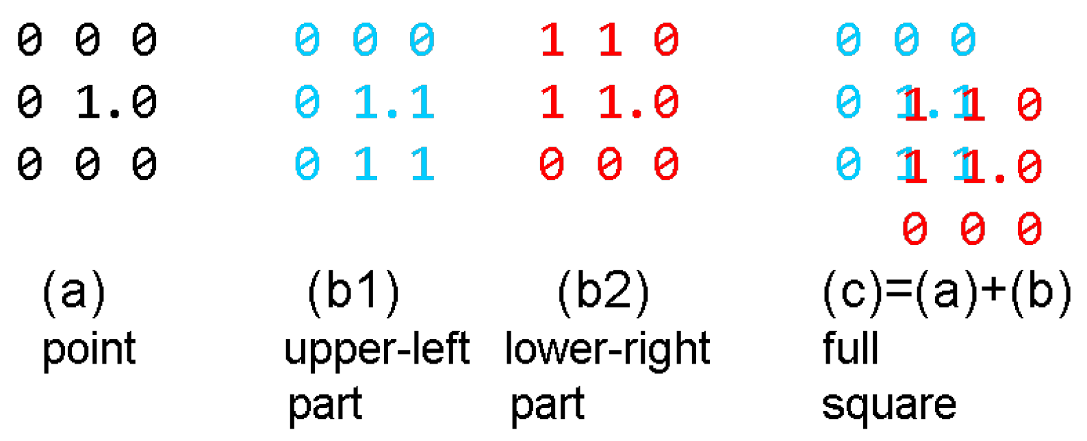
2.4. Sample Pattern: Squares and Points
In this section, we demonstrate that the GA can produce optimal “square/point” patterns (SP patterns) defined by three tiles. The pattern contains simple 1-points and squares
surrounded by zeroes. In order to keep the computations as local as possible, we restrict the size of the tiles to
. The designed three tiles are shown in
Figure 1. The
point tile (a) is just a 1 surrounded by 0’s. The center is marked and is the anchor/origin of the tile. A square surrounded by zeroes can easily be defined by a
tile, but not by a
tile. Therefore, the square is composed of two parts (b1) and (b2), which then aggregate to a full square (c) (without 2 zeroes at two of the corners) during the GA evolution.
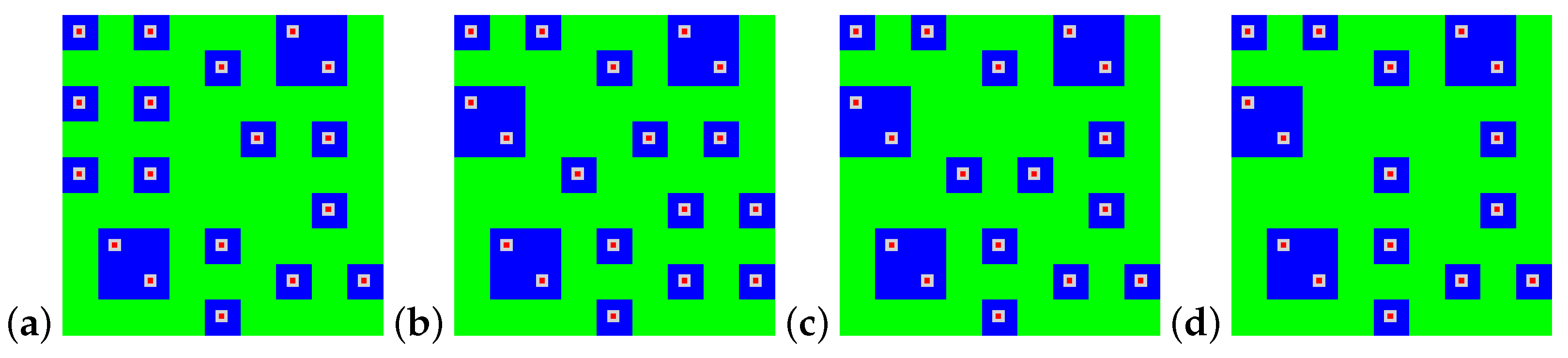
Some solutions of the GA are shown in
Figure 2. The tile matches are marked. All patterns are valid as desired (show only squares and points surrounded by zeroes) and each cell is covered (the field is fully covered). Patterns (a) and (b) are optimal with a maximal possible number 18 of matches. (a) Contains 2 squares and 14 points, whereas (b) contains 3 squares and 12 points. Patterns (c) and (d) are non-optimal with respect to the number of matches.
2.5. Tiles for Generating Loop Patterns
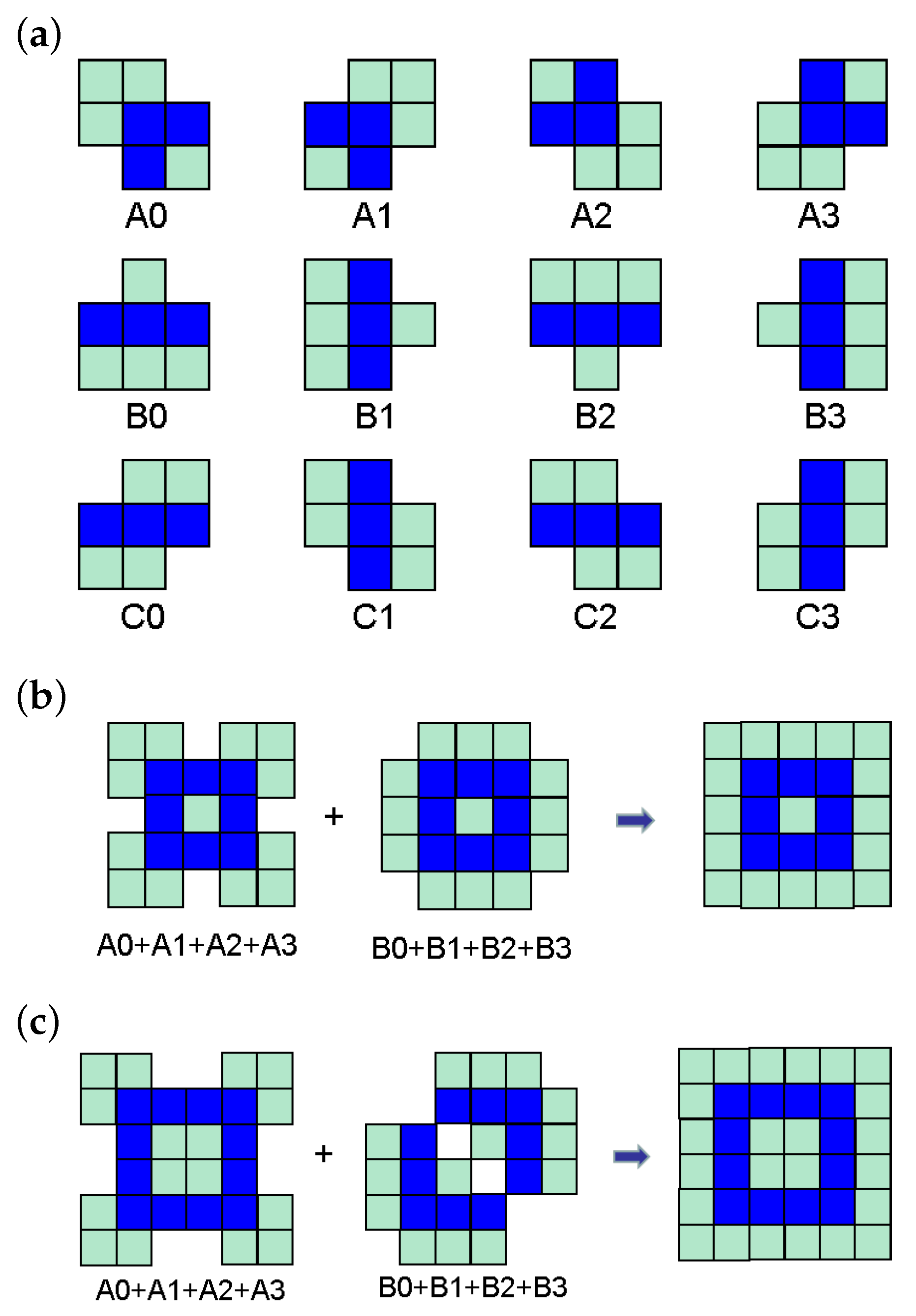
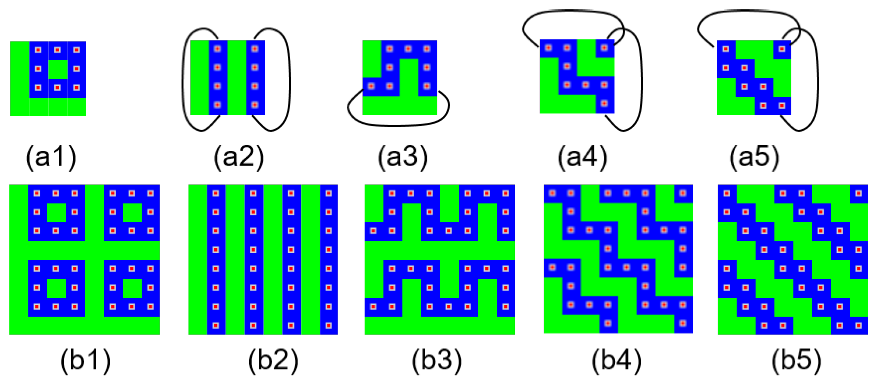
Now, we want to generate a loop pattern using the GA. A set of 12 tiles was designed specifying such patterns (
Figure 3a). The size of the tiles was restricted to
. The tiles were designed in the following way: (1) possible loop patterns were constructed on a grid (the
aimed patterns). (2) The aimed patterns were scanned by small windows at several relevant positions. Such
window patterns were stored or remembered. (3) Tiles were designed that can cover the window patterns and that can overlap.
The tiles A (
Figure 3) define corners, B define straight continuations, and C define possible turns. The null pixels are necessary in order to enforce connections. Simply speaking, the tiles’ surfaces need properly structured interfaces in order to aggregate. At the moment it is not clear how the interfaces can be defined in a methodical way.
Figure 3b,c shows how certain small loop patterns can be assembled by tiles. A small open square (
Figure 3b) can be formed as shown by (A0 + A1 + A2 + A3) + (B0 + B1 + B2 + B3) where ‘+’ means adding a tile or compound tile that overlays without conflict. The resulting composition can fit into a cyclic field of size
or
. A larger open square (
Figure 3c) can be formed as shown fitting into a cyclic field of size
or
.
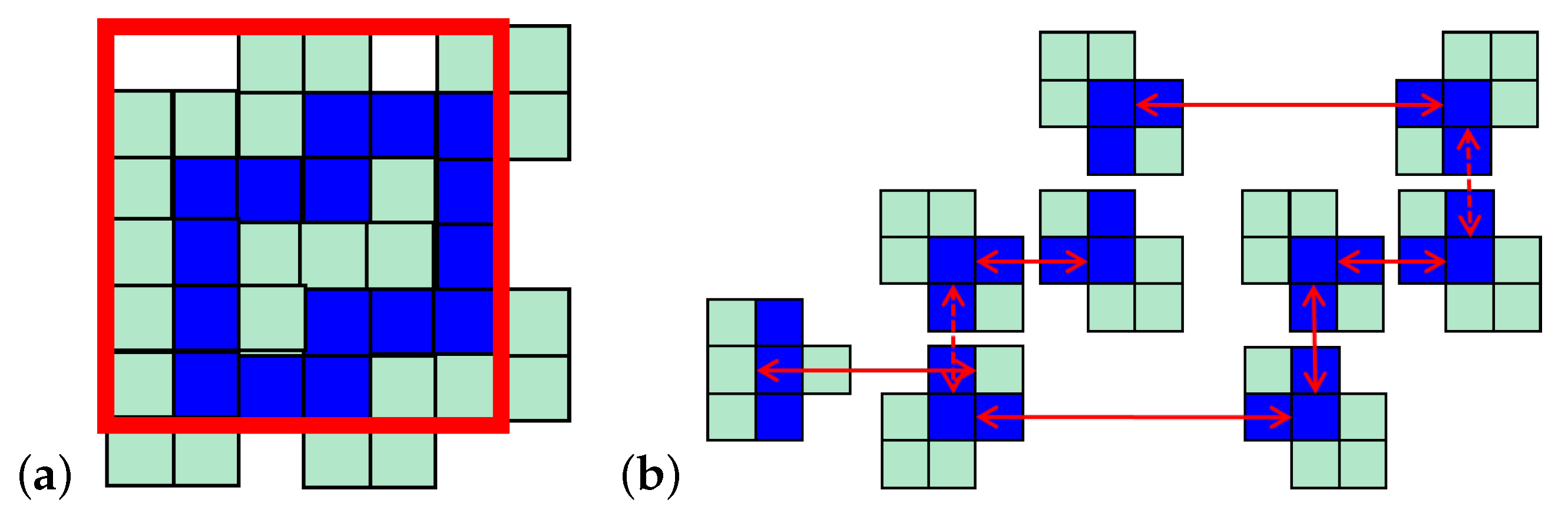
Figure 4 shows (a) another small loop and (b) how it can be assembled by tiles.
Until now, it seems difficult to automate this process, and therefore, it is a topic of further research. It is also a question of what is a minimal set of
tiles, or what is the smallest size of the tiles in order to produce the same class of patterns. Note that there are different classes of loop patterns that differ in certain details like allowed crossings (and how) or allowed diagonal connections. We discuss here only the class of loop patterns that are defined by the tile set shown in
Figure 3a.
2.6. Loop Patterns Generated by GA
Let us consider generated patterns of size
. We consider patterns as ‘equal’ if they are equivalent under rotation, shift, or mirroring. For
, there exists only the loop pattern
, and
for
. Note that a straight line of one-pixels forms a loop under cyclic boundary conditions. For
, there exist five patterns as shown in
Figure 5a1–a5. All patterns contain one loop, except (a2), which contains two loops. Patterns (a4) and (a5) use two cyclic connections each, one horizontal and one vertical. The patterns (b) are the patterns (a), doubled vertically and horizontally, altogether they form quadruplicates, and that is why we call them
quad patterns or simply
quads.
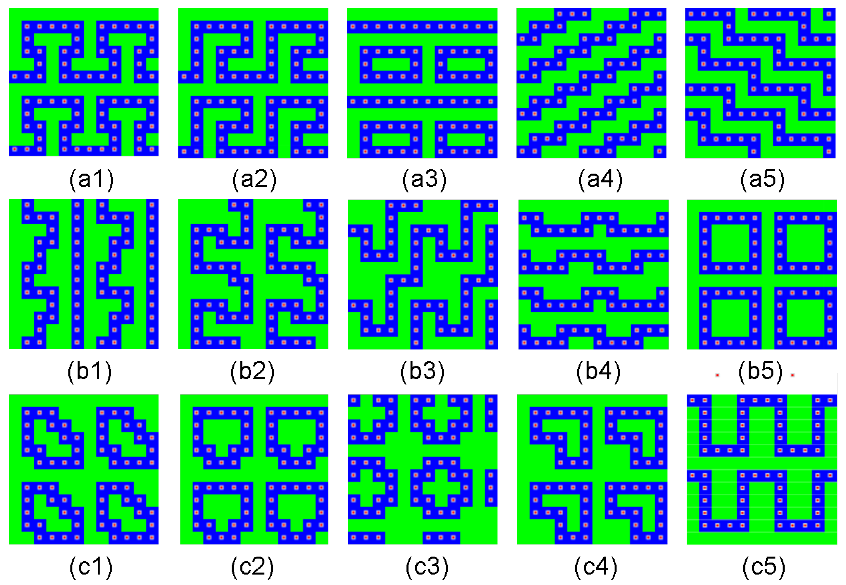
For
, some of the GA evolved patterns are shown in
Figure 6 as quads. The patterns (a) have the same number of 1- and 0-pixels, and therefore, we can call them
balanced. They are also very
dense if we consider 0-pixels as space between the 1-pixel loops. Patterns (b, c) are less dense, because their loops are more commodiously embedded in the space. The used GA favors dense patterns, but it could be modified to aim at low-density loop patterns.
Figure 6a3,b1,b4 show two loops, and the other patterns only one. Patterns (b5, c1–c4) contain plane loops. Pattern (a3) contains a plane and a straight loop, (b1) a wave and a straight loop, and (a1, a2, a4, a5, b2, b3, b4, c5) are wave loop patterns.
The GA does not always produce loop patterns (
Figure 7). GA generated
optimal patterns are patterns with a maximal number of tile matchings. Such patterns correspond to dense loops, as shown in
Figure 6a1–a5, and their number of one- and zero-pixels is balanced (may differ by one if the whole number of pixels is not even). The generated non-optimal patterns, in which the number of tile matches is not maximal, can be (a) loop patterns, or (b) faulty loop patterns. We can observe special types of faults that may appear in combination (
Figure 7).
Remark. In the course of the further GA evolution of the (b4) pattern, the uncovered cells can be eliminated such that only line loops will appear. In (b5), a tile can be added, closing the gap and thus forming connected loops.
It is a matter of definition what kind of loops are allowed. It would be possible to modify the fitness function of the GA in a way that (a) TCN and certain ART structures are suppressed (adding a penalty to the fitness function); (b) 3PN and/or 4PN are promoted (adding a reward); (c) UFC are allowed in a certain range in order to control the space between loops.
For
, some of the GA evolved patterns are shown in
Figure 8 as quads. The patterns contain one loop (a), two loops (b1–b5), or three loops (b6). The patterns (c) contain connected loops. Loops are connected through connectors. A connector with four pins is used in (c1–c5), and one with three pins in (c6). We find
windows marked in the quads intended to exhibit the inherent structures. In order to show explicitly the loops for the original
patterns (as marked) external connections as added in
Figure 5 would often be necessary. Some of the loops cross the
window boundary back and forth, e.g., (a4) and (b5). Most of the loops in the loop patterns are wave loops.
We have seen that a GA can generate patterns of a certain class (such as square/point, loop, defined by a set of tiles). The GA uses a globally defined and tested fitness function, here given by the number of tile matches. It was a kind of surprise that such complex patterns can easily be found by the GA although the search space is very large. The fitness function can easily be modified, for instance, including further conditions like the ratio between zero and one pixels (density), the length of loops, the kind of loops, and so on. Therefore, the GA is a powerful tool for generating patterns under complex global conditions. In the next sections, we want to show that loop patterns can also be generated by testing only local conditions by a CA rule.
3. Generating Loop Patterns with a Probabilistic Cellular Automata Rule
In the following
Section 3.1, we want to decide what kind of updating scheme and rule we will use, then, in
Section 3.2, how the tiles from the already tile set are incorporated into the CA rule (by templates derived from them), and then in
Section 3.3, we will describe the rule that injects noise when a loop pattern is not reached. Simulations follow showing the resulting patterns.
3.1. Choosing the Type of the Rule
The simulation of a CA is very simple, that is one reason why CA are so popular. Nevertheless, there are different types of CA and we need to choose the best-suited one for our application. There are two important properties we have to choose: (i) synchronous or asynchronous updating, and (ii) a deterministic or a probabilistic rule.
(i) Synchronous or Asynchronous Updating.
Synchronous updating.
(Phase 1) For every cell its new state is computed by a local rule and buffered in the new state variable .
We use z to denote that a variable z (with memory) is used to store the value v.
(Phase 2) The state of each cell is updated (replaced) by its new state.
It is important to notice that the order in which the cells are processed in phase 1 and in phase 2 does not matter, but the phases must be separated. This model can easily be implemented in software, or in clocked hardware using d-flipflops (internally supplying a master and a slave memory).
Asynchronous updating.
There are several schemes. In the pure case, there are no phases. A cell is selected at random, is computed, and then immediately updated: .
We want to use the following scheme. A time step is considered as a block of micro time steps . A selected cell is processed during one micro time step. For each time step, we select the cells sequentially in a different random order (elements are mutually exclusive). During one time step, each cell is updated once, but the order is random. We display CA configurations at time steps. This scheme is called random sequence or random new sweep.
(ii) Deterministic or Probabilistic Rule. A deterministic rule always computes the same next state for a given input (the combined state of all neighbors). A probabilistic rule computes different next states with certain associated probabilities for a given input.
Combination. In principle, we can combine synchronous or asynchronous updating with a deterministic or a probabilistic rule. This makes four options: (1) synchronous updating and deterministic rule; (2) synchronous updating and probabilistic rule; (3) asynchronous updating and deterministic rule; (4) asynchronous updating and probabilistic rule.
Option 1: Until now, it was not possible to design such a rule that can produce loop patterns. The problem is that the evolving patterns may get stuck in non-desired patterns or oscillating structures such as we know from the Game of Life. It remains an open question if it is possible to find such a rule.
Options 2–4: These options are related because the computation of a new configuration is stochastic. It seems that they can be transformed into each other to a certain extent. We decided to use option 4 (random sequence together with a probabilistic rule) as in our former work [
1,
2,
3,
5]. With asynchronous updating, we do not need buffered storage elements and a central clock for synchronization, which is closer to the modeling of natural processes.
3.2. Templates Used for the CA Rule
One of the key ideas is to use templates (local matching patterns) for testing them everywhere (at any point ) in the CA space. If we find a template match we call it a hit. A hit means that the cell is covered by a pixel of a tile. We are searching for stable patterns where we have at least one hit everywhere.
A template is a shifted tile. Let us assume that templates have the size of pixels. We have chosen m to be odd because then it is easier to define the unique center as the origin for the local coordinates and to handle symmetric templates. But this choice is not obligatory as long as all templates fit into the boundaries of . We index tile and template pixels relative to their center located at . We declare x-coordinates to increase rightwards and y-coordinates downwards.
For a given tile (the generating tile), we derive a set of templates by shifting the generating tile vertically and/or horizontally. We consider only the valid pixels with a value of 0/1 for the process of deriving the templates. We call a valid pixel reference pixel when it is selected for deriving a specific template. For each reference pixel with the (relative) coordinates , we shift the tile in such a way that after shifting, the reference pixel occupies/arrives at the center of the derived template, i.e.,
for each reference point i at
where the operator shifts a tile L by the given offsets, and is
shifting-in null pixels and deleting shifted-out pixels.
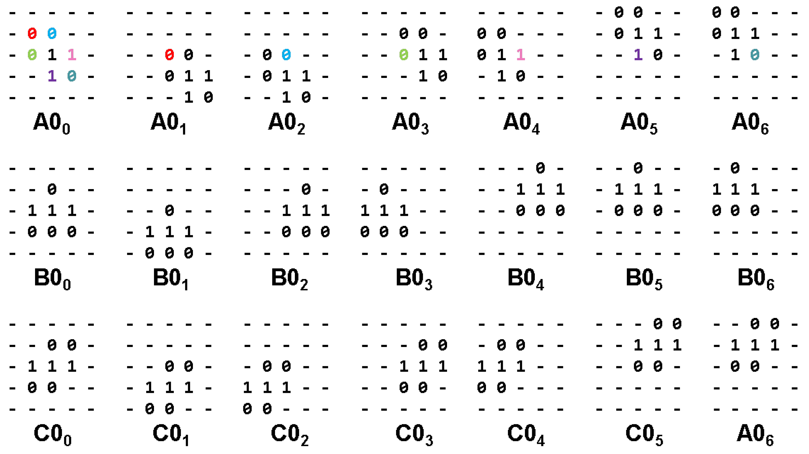
Figure 9 shows the templates derived from
,
B0, and
as defined in
Figure 3.
is the generating tile and also the first (the main) template that needs no shift because it contains a valid pixel in its center already (what we assumed). Now, we consider the pixel A0 (−1,−1), in green. A0 is shifted by
steps, (1 rightwards, 1 downwards), which yields
.
is A0 shifted by
, where the red pixel occupies the center.
is A0 shifted by
, and so on. As a result, we obtain seven templates derived from
. In a similar way, we obtain seven templates each from
and
. As we have altogether 16 tiles with 7 valid reference pixels we obtain
templates. We may reduce the number of templates by joining them using classical methods of minimization logical functions where the center value is the output and the neighboring pixels are the inputs. The templates (to fit in a square array) are larger than the given tile because of shifting, the radius of the templates is twice the radius of the given tile.
Remark. In general, we can define a template set independently of certain tiles, but this is a general topic that will not be followed here.
3.3. The CA Rule
The following rule is able to evolve CA loop patterns. The main idea is to inject noise if no template hit is recognized in order to drive the evolution to a stable pattern. In such a pattern, there is everywhere a template hit, i.e., every CA cell is either equal to the center of a tile or it is a part (a pixel) of a tile, corresponding to the center of a template.
The default value of the new state
is the current state
s. All templates
are tested against the current CA neighborhood at the selected site
where the template center is excluded from the test. If there is a template hit, the center of the template defines the new state. (Either the CA neighborhood corresponds fully to the template or only the center is false and then it is corrected). Noise is injected under certain conditions including certain probabilities. The main condition is
, which becomes true if there is no hit. The condition
takes toggling uncovered cells of the NESW-neighborhood into account in order to dissolve them. The additional condition
excludes faulty loop patterns.
wherehit() is a test whether a template
matches in the current CA neighborhood of the selected CA cell
:
Remark. For specialized rules, it may be useful to store the number of template hits in the state of the cell:
. Certain values of
h were used to inject additional noise [
2,
5] in order to find a minimal or maximal number of dominos covering a space.
is the value of the center pixel of a template match. Here, the value of the last hit is used, if there are several hits. It would be possible to use the value of the first hit or that of any hit randomly. To which extent the choice matters is a topic of further research.
is the main basic condition that drives the evolution through injecting noise if there is no hit, which means that such a cell is not covered by a tile pixel.
- –
is a function that is TRUE if a trial is successful under probability , otherwise FALSE. In Python, the function can be defined as: “def decision(probability): return random() < probability”
This additional condition avoids lonely uncovered cells that cannot be destroyed by
. This problem will further be discussed in
Section 3.5.
- –
is the North-East-South-West-Neighborhood (relative indexes)
- –
is a function that tests for each neighbor in the Neighborhood (set of relative positions of the neighbors) a local condition ConditionForANeighbor and counts the fulfilled conditions.
These additional conditions realize the loop path condition. Thereby faulty loops are excluded (see end of
Section 3.6).
This alternative additional condition allows unconnected and connected loops.
The behavior of the CA rule depends on the probabilities . We can use them as parameters in the general rule: . Note that the conditions have to be fulfilled to drive the evolution to a stable pattern by destroying uncovered cells. The condition can be deactivated by setting .
3.4. Simulation of the First Rule
The
First Rule (also called
Basic Rule) is the
in which we used the probability
. It injects noise only when the own cell shows no hit, i.e., the cell is uncovered.
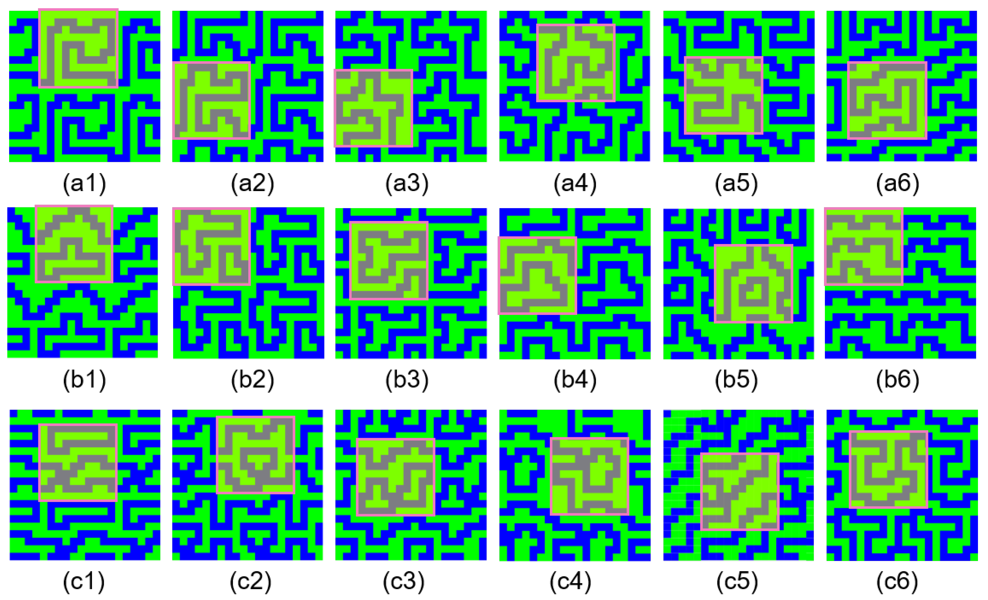
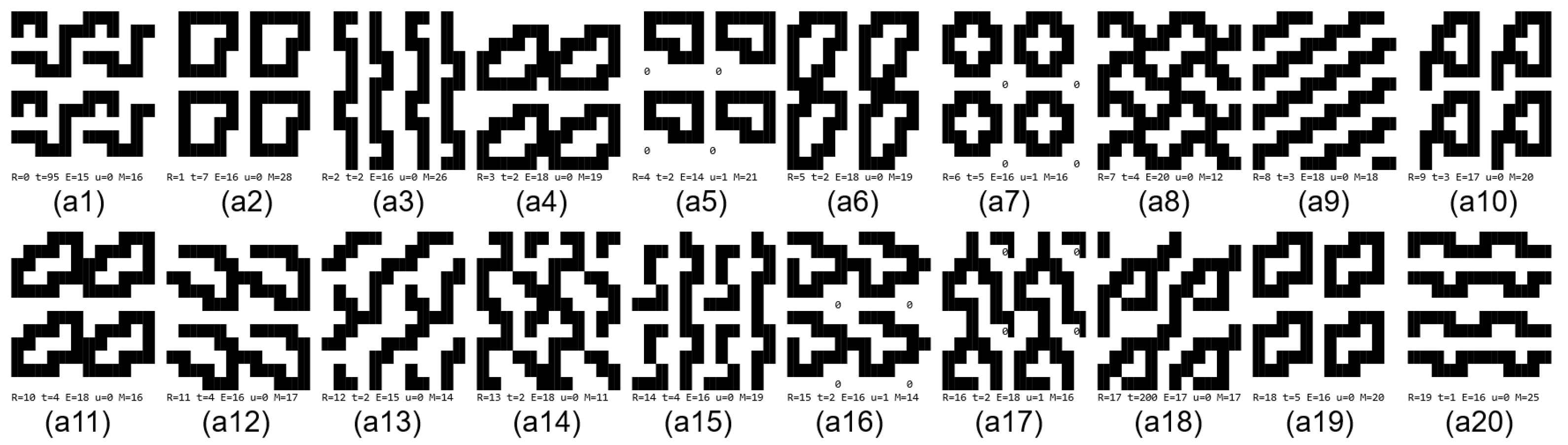
Figure 10 shows the evolved patterns for 20 runs with different random initial conditions. We found different types of patterns:
Seven patterns (a2, a3, a5, a7, a9, a19, a20) with unconnected (separated) loops, patterns that we mainly aim at.
Four patterns (a4, a6, a8, a11) with loops that are connected, meaning that there are connections between them. It is a matter of definition whether such loops should be within the scope of objectives. In
Section 1.2.2 we classed them as faulty patterns.
Nine patterns (a1, a10, a12, a13, a14, a15, a16, a17, a18) are faulty loop patterns. Such patterns are not really what we want to achieve.
Four patterns (a5, a7, a16, a17) contain an uncovered cell, marked by ‘0’. Such cells are toggling () because of noise injection through condition . Such patterns can also be of interest but they are partially unstable (cycling). We may wish to exclude them, or we may fill the toggling cell constantly with zero to yield a lower-density loop pattern with less ones.
Although this is only a test case (the number of types and the actual pattern may vary) we can observe that the First Rule does not work perfectly because a faulty loop pattern can appear. Now, we aim at a rule that produces a loop pattern only. First, we want to avoid uncovered toggling cells (type 4 patterns) by the enhanced
Second Rule described in the next
Section 3.5. Then, we want to avoid faulty patterns of type 3 and type 2 (
Third Rule,
Section 3.6).
3.5. Simulation of the Second Rule
The Second Rule is the , it was used with the setting . It avoids the toggling of uncovered cells. The problem was solved by injecting additional noise from a neighbor to the current cell if there exists a neighbor that is uncovered (with no hit). We have used the NESW neighborhood for this problem. This is achieved by activating the condition by setting the probability . We recall the condition . Indeed we could not find such lonely toggling cells in the many simulation experiments. This is not proof that the NESW neighborhood is sufficient in general to solve this problem. In the general case, a larger neighborhood is probably necessary if sophisticated or larger tiles are given.
Remark. We may consider a situation where the given tile(s) cannot cover the space. Given a square tile of size with a black border of width one around a white square of size . The tile shall be used to cover a field of size . We can easily see that only one such tile can be used (because of overlaying conflicts) and there will always remain uncovered cells. In such a case, it would even be better to use the First Rule in order to reach a partially stable pattern, in this case with one tile only.
3.6. Simulation of the Third Rule
The Third Rule is the , it was used with the setting . In addition, it activates the condition
-
(Case 1) , or
-
(Case 2) .
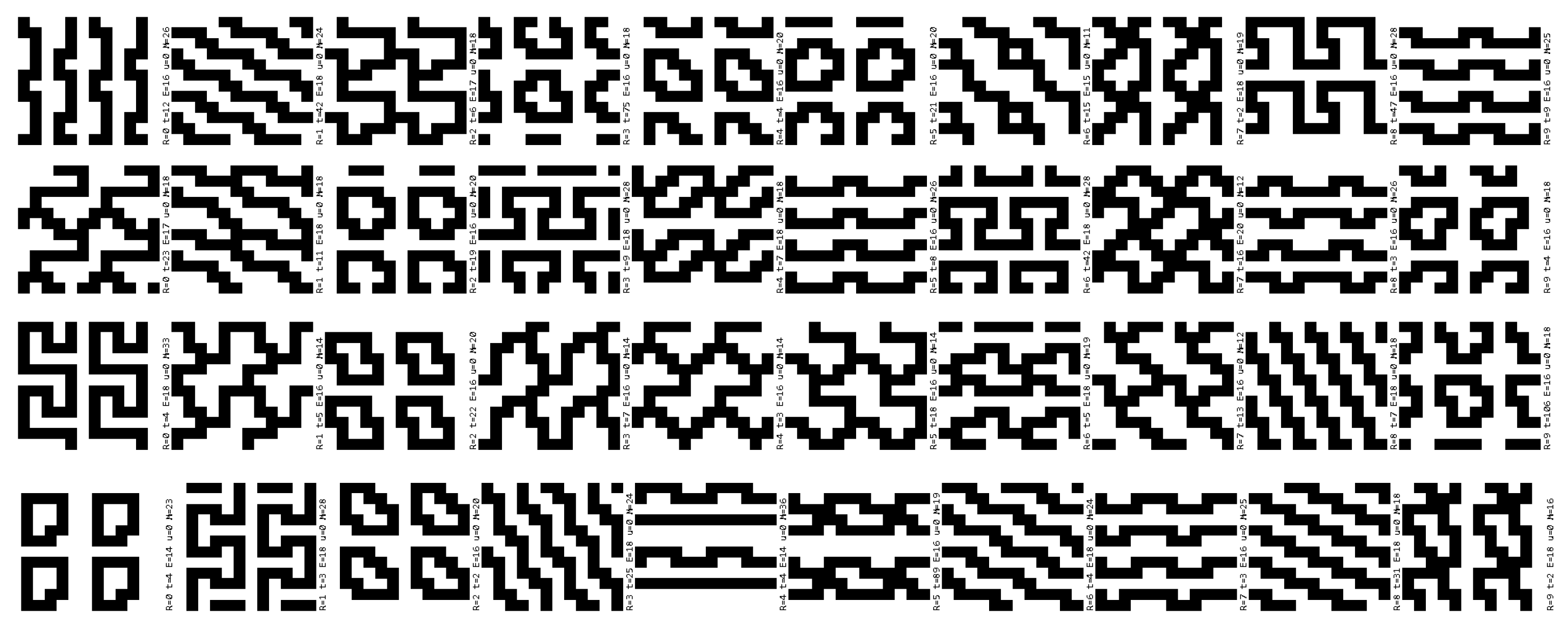
(Case 1) Additional noise is injected if the number of ones in the NESW neighborhood is less than 2. This means that only patterns are allowed in which a one-cell has at least two orthogonal one-neighbors. Thereby faulty type 3 patterns of the First Rule simulation are excluded, but connected loops (type 2 patterns) are still allowed. Many simulations were performed (
Figure 11) converging to loop patterns with separated loops or patterns with connected loops having 3- or 4-pin connectors.
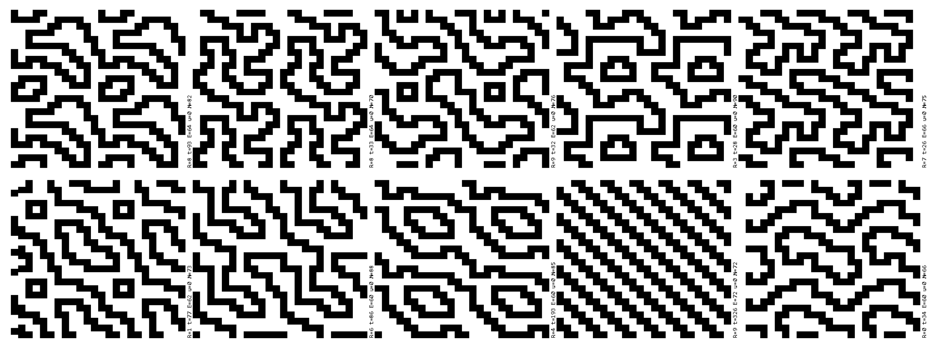
(Case 2) This condition is the negation of the loop path condition (a path cell has exactly 2 path cells in NESW). Noise is injected if this condition is not fulfilled. Thereby the evolution is pushed to loop patterns
only (
Figure 12), the patterns we aimed at.
4. Discussion and Future Work
4.1. Forming Loops by the Tiles
We defined a set of overlapping tiles that are able to cover a 2D space in a way that a loop pattern can appear. For the design, it was important that the tiles can connect to each other by overlapping in a way that they can find other suitable tiles in the continuation of a path (during the evolution), and finally that the beginning and end of a path connect with each other and form a loop.
The driving force in the GA is the number of matches. Let us consider an almost closed loop (or we may call it a slightly opened loop), just one path cell is missing (is zero). Compared to the (closed) loop there are fewer matches because the endings are “free”, not connected to tiles that could be used to close the gap. Then, the GA closes the gap because it tries to maximize the number of matches through using more tiles.
The CA rule works differently because it tries to avoid uncovered cells. In the case of an almost closed loop, there are uncovered cells around the gap (if the tiles are properly designed). The gap is then closed by evolution; finally, all cells are covered, no more noise is injected and the pattern remains stable. These are only rough explanations that have to be detailed and improved in a further work.
4.2. The Genetic Algorithm Generating Loops
A GA was developed that can find optimal loop patterns based on the set of tiles. It tries to maximize the number of tile matches. Some of the patterns are faulty (e.g., touching black cells on the diagonal, loops having branches). This means that the designed tiles are not able to produce loop patterns only but also faulty ones. Instead of improving the tiles to make them proper in a way that loop patterns are evolved only, this issue was left to the CA rule (with condition ). Nevertheless, it is a research issue to find a proper set of tiles that enforce the forming of loop patterns only.
4.3. The Cellular Automata Rule Generating Loops
A CA Rule was defined that tests templates derived from the defined tiles. In the first version (First Rule, Second Rule) it can easily evolve loop patterns or faulty ones. The extra logical condition
can exclude the faulty ones (Third Rule). This condition can easily be modified in order to allow connections between loops. A difficulty during the design and simulations was to make the rule simple and reliable. The used settings for the probabilities
were good working, but there is potential for optimizing them in order to minimize the average time for finding a stable pattern. For small problem sizes, the CA rule converges fast, but for large sizes, we expect an exponential increase, as already tested for domino patterns in [
2]. In order to reduce the computational time, the CA rule programming code can be optimized or other techniques (e.g., divide and conquer) could be involved.
4.4. Future Work
There are several open questions.
What are (all) possible loop patterns depending on the size of a field, and what is the distribution of different loop types with certain properties?
A special question could be: How many loops (optionally restricted to a certain type) can maximal be placed in a certain field.
Can it be proven that the presented CA rule always (for large field sizes) produces stable loop patterns? What are the probabilities that certain loop types are evolved? What happens for large fields?
For this mainly experimental work, the minimal loop pattern size is
, and we see no limit for large sizes. For large sizes, we expect a mixture of different loops and loop sizes as in
Figure 12. The CA rule always generated stable loop patterns so far, but the computation time increases exponentially. In the simulation, rectangular fields could be handled too. Nevertheless, the convergence and limits of this approach should be proved and further evaluated.
How do tile matches lead to loops? The tiles were designed in a way that corners and lines can easily connect/overlap to a loop that is surrounded by zeroes. The tile matches are maximized, thereby each cell tries to obtain a match, and the idea used is that loops are paths with a maximal number of matches. Until now, the defined set of tiles did not always produce loop patterns, and therefore the CA rule needed an additional local condition (the path condition). This issue has to be further investigated, and it is the aim to find a proper set of tiles that securely stimulates the generation of loop patterns.
How can optimal loops be generated on the basis of local conditions only when optimality depends on a global measure. Possible parameters for a global measure are:
- –
The space between loops;
- –
The number of loops;
- –
The length of the loops;
- –
The type of the loops (plane, straight, wave).
We can conclude that we found a way to generate loop patterns using local conditions only, but there are several open questions to be answered in further research.


