Abstract
The hybrid model for analyzing distortions of a laser beam passed through a moderately scattering medium with the number of scattering events up to 10 is developed and investigated. The model implemented the Monte Carlo technique to simulate the beam propagation through a scattering layer, a ray-tracing technique to propagate the scattered beam to the measurements plane, and the Shack–Hartmann technique to calculate the scattered laser beam distortions. The results obtained from the developed model were confirmed during the laboratory experiment. Both the numerical model and laboratory experiment showed that with an increase of the concentration value of scattering particles in the range from 105 to 106 mm−3, the amplitude of distortions of laser beam propagated through the layer of the scattering medium increases exponentially.
1. Introduction
Currently, optical diagnostic techniques are essential experimental tools employed in a large and diverse set of research and industrial applications. Based on measurements of scattering intensity and light extinction, a number of these techniques are able to determine the parameters of scattering particles, such as size, shape, and concentration [1]. Examples of applications are numerous: in meteorology, the measurement of atmospheric constituents is performed by analyzing the backscattering light signal via the LIDAR (Light Detection and Ranging) technique [2]. In oceanography, marine picoplankton is characterized from the laser light scattered by the illuminated particles [3]. The optical radiation is actively used in various bio-medical applications as a non-invasive diagnostic tool, as well as to treat a number of diseases [4]. During the past three decades, the investigation of laser light propagation in skin tissue and the human brain has been particularly extensive [4,5,6,7,8,9,10]. In combustion engineering, a variety of laser-based diagnostics have been developed over more than three decades in order to determine the physical properties of fuel droplets from atomizing sprays [6]. These optical measurements are of fundamental importance in the improvement of combustion efficiency and in the reduction of pollutant emissions from modern internal combustion engines and gas turbines. Another field where optical diagnostic techniques are of particular significance is free-space transmission of energy or information, namely, free-space optical communications, wireless energy transfer through the scattering and turbulent atmosphere, imaging objects through scattering atmospheric aerosol, space debris removal, etc.
One of the limitations of the optical techniques is related to the radiation attenuation and scattering. Under optically thick conditions, the scattering can significantly decrease the quality of the beam and thus introduce errors in measurements. However, it is necessary not only to simulate the propagation of the radiation through the medium but also to establish techniques to measure the beam distortions introduced by that medium.
Measuring laser beam distortions is one of the existing problems that has to be solved. Another problem that is also of great importance is compensating measured distortions. As is known, in a turbid medium, a part of a laser beam energy is absorbed while the rest is scattered. This scattered light makes objects look blurred and degrades beam-focusing efficiency. There are a wide variety of applications for which the solution of the problem is very important, i.e., wireless data transmission, pattern recognition, and medical noninvasive diagnosis, among others [11,12]. The wavefront-shaping technique to focus the radiation that propagates through a strongly scattering layer was developed back in 2007 [13]. The authors used the SLM and were able to properly shape the wavefront to focus the radiation through scattering objects. Various techniques have been developed since 2007 to resolve the focusing of light through scattering media [14,15]. Authors of [16] showed the ability to obtain clear images of objects by means of holographic techniques that reverse a scattering process. Authors of [17] use coherence and spatial gating to produce images of optical properties of a tissue up to 9-mm deep with millimeter-scale resolution via a technique known as multispectral multiple-scattering low-coherence interferometry. Imaging of fluorescent objects when the space behind a scattering medium is limited can be achieved using the technique described in [18]. SLM can be used to obtain images of objects located within or behind a scattering layer [19,20,21,22]. In [23], authors demonstrated a steady-state focusing of coherent light through dynamic scattering media. In [24], authors demonstrated the use of the method of inversion of transmission matrix. They proved that the focus’ peak-to-background intensity ratio can be higher compared to conventional methods. In [25], the authors proposed a new technique that allowed for the 204-fold increase of the peak-to-noise ratio. Another group of scientists proposed the system that uses the full-polarization optical digital-phase conjugation and doubles the peak-to-noise ratio [26]. In [27], programmable acoustic optic deflectors were used to obtain the images of the targets in the living tissue. Bimorph deformable mirrors, as well as stacked-actuator mirrors, are also used to increase the radiation energy in the far field while focusing a laser beam through a scattering medium [28,29,30], turbulent medium [31,32], or a pinhole [33] for free-space optical communication systems. Spatial-light modulators are widely used in different areas of research; their use is not limited to the imaging and focusing applications only. Spatial-light modulators also show vast potential in such applications as micro- and nano-scale fabrication [34], and laser beam shaping [35,36].
In this particular paper, we will not concentrate on the problem of compensating distortions. Instead, we present the hybrid model for (1) The simulation of laser beam propagation through the moderately scattering medium using the Monte Carlo technique; and (2) Measuring distortions obtained by the laser beam by means of the numerical model of the Shack–Hartmann sensor. The proposed model was briefly mentioned in the authors’ previous paper [37], which was devoted to the compensation of measured laser beam distortions using bimorph deformable mirrors. In this paper, we would like to describe the proposed model in detail and provide the results of the numerical analysis, as well as the experimental validation of the model.
The research is organized as follows. First, a radiative transfer equation and its possible solutions are presented. Second, a Monte Carlo technique to solve the radiative transfer equation is described; its software implementation and verification are provided. Third, the Shack–Hartmann principle is explained, and the developed numerical model is described. Fourth, the laboratory experimental setup with the Shack–Hartmann sensor is shown. A comparison and discussion of numerical and experimental results obtained are presented.
2. Materials and Methods
2.1. Radiative Transfer Equation
Estimation of radiation attenuation and multiple scattering effects requires knowledge of the radiative transfer of optical energy through the medium [1]. In the field of optical diagnostics, the radiative transfer equation is commonly used to describe the photons transport, specifying a balance of optical energy distributed between the incident, outgoing, absorbing, and scattering radiation propagated through the medium. The radiative transfer equation is presented below:
where I is a radiance in the particular direction (either s or s’), t is time, is the vector position, is the incident direction of propagation, μe is an extinction coefficient [38,39], and μs is a scattering coefficient. This is a value inverse proportional to the distance on which the collimated light flux will be reduced due to the scattering [40,41]. is the scattering phase function derived from the appropriate scattering theory (e.g., Mie or Rayleigh theory), d is the solid angle spanning , and c is the speed of the light in the surrounding medium.
In other words, Equation (1) can be explained as follows: The resultant radiance along the direction is a sum of the scattered radiance coming from all directions to the direction and the radiance loss due to the absorption. The total extinction represented by the first right-side term of Equation (1) describes two processes that contribute to the total resultant radiance, namely the radiance loss due to the scattering process and the radiance loss due to the absorption process. Though the radiative transfer equation can be applied for a wide variety of media, the analytical solution of this equation is available for rather simple circumstances with different assumptions. Thus, techniques such as the method of path integrals, diffusion approximation, light scattering by Brownian particles [42], and the method of the small-angle approximation [43] were developed.
Nevertheless, the techniques mentioned above are supposed to be used under different assumptions and simplifications. For example, the methods of light scattering by Brownian particles, as well as the diffusion approximation, only suit the small anisotropy factor-scattering media. The method of small-angle approximation does not consider the diffusively scattered light and cannot be applied to our task because the idea of the research is to analyze the influence of both quasi-ballistic and diffusive components of the scattered radiation. The method of path integrals has two variations: analytical and stochastic. Analytical method is basically the modified method of Brownian particles, whereas stochastic method is Monte Carlo method. As is known, Monte Carlo technique [44,45] is the most versatile and widely used numerical technique that provides an approximate solution of the radiative transfer equation for the vast majority of conditions.
2.2. Monte Carlo Simulation
The Monte Carlo technique is a widely used approach toward sampling probability density functions for simulating a wide range of problems. The first use of the method for photon transport in biological materials was Adams and Wilson in 1983, which considered isotropic scattering [46]. Keijzer et. al. introduced anisotropic scattering into the Monte Carlo simulation of biological tissues, implementing a simulation that propagated photons using cylindrical coordinates, which introduced the Hop/Drop/Spin nomenclature for organizing the program [47]. Prahl et al. reformulated the program using photon propagation based on Cartesian coordinates, which made the program much simpler to convey in written form [48]. Wang and Jacques adapted and augmented the work of Keizer and Prahl to write the Monte Carlo Multi-Layered (MCML) program that considers tissues with many planar layers with different optical properties [8].
Monte Carlo technique simulates the behavior of the elementary parts of a physical system. In regards to light propagation through a medium, this technique uses quantum nature of light and simulates the propagation of photon flux [49].
In general, there are two Monte Carlo techniques: corpuscular and wave [50]. Both methods have their advantages and disadvantages.
The “Wave Monte Carlo” treats the propagation of radiation as a wave propagation. It describes the propagation of a wave through a set of screens that contains scattering particles. The resultant wave becomes stochastic due to the interference between the unscattered and scattered waves. As a result, we get the complex amplitude of the random field. An ensemble of the obtained fields for the statistically independent sets of screens is the calculated intensity distribution. This technique is particularly applied for the mono-direction radiation.
In contrast, the “Corpuscular Monte Carlo” treats the propagation of radiation as a corpuscula (photon) flux. This technique performs the statistical calculation of the ensemble of photons—the average number of photons depending on the coordinate equals to the intensity distribution. “Corpuscular Monte Carlo” is applied for both the weakly and strongly scattering media. Another feature of this method is that it is not supposed to model the fixed position of the scatterers. It instead models the events of the photon–particle interaction with the desired probability density. From this point of view, the Brownian movement of scatterers is considered in the simulation by default.
Choosing each method is a matter of opinion, since both show similar results [50]. We have chosen the “Corpuscular Monte Carlo” technique for our simulation.
First, we simulated the initial uniform intensity distribution of a laser beam with diameter equal to 4 mm and wavelength equal to 0.65 µm. The random number generator was used to calculate the initial position of each of the 2.5 × 10¹¹ photons within the beam aperture. Afterward, we calculated the trajectory of propagation of each photon through the 5-mm layer of scattering medium consisted of a monodisperse spheres of 1-µm diameter and refractive index of 1.582 (refractive index of the medium was 1.33). The influence of relative refractive index is rather complicated [51]. For small particles, the influence on the forward-scattering signals is mainly due to the part of the internal reflection if the relative refractive index deviates from 1. However, when the relative refractive index is close to 1, the effects on the forward-scattered light from both the surface reflection and internal reflection are great. For large particles, the contributions of the surface reflection and the internal reflection to the forward-scattered light are much weaker than the diffraction when the relative refractive index deviates from 1. When the relative refractive index is very close to 1, the effects on the forward-scattered light from the internal reflection are great.
The absorption coefficient for such conditions (i.e., for the selected wavelength and refractive index) will be negligible according to [52]. Thus, no absorption will appear, and we do not have to track whether a particular photon should be excluded from the simulation. The concentration value, or a number of spheres per cubic millimeter, of the scattering suspension was varied approximately from 105 to 106 mm−3.
In order to define the trajectory of the photon, three key parameters have to be calculated. First, free path length l—the distance between two scattering events or between two sequential interactions between the photon and a particle (Equation (2)). Second, scattering angle θ—the angle between the current and the new direction of photon’s propagation (Equation (3)). Third, azimuthal angle φ—the angle between the projection of the new direction on the plane perpendicular to the initial direction of the photon’s propagation (Equation (4)).
where —random numbers uniformly distributed within the interval [0, 1), µs—scattering coefficient, g—anisotropy factor.
The direction of photon after a scattering event is defined by scattering diagram or phase function [53,54]. The phase function is a function of the probability density of scattering in the direction s’ of a photon moving in the direction s, i.e., a function that characterizes the elementary act of scattering. In other words, the phase function describes the angular distribution of the intensity of light scattered by an elementary volume. The shape of the scattering diagram depends on the wavelength of the incident radiation, the size of the scatterer, and the relative refractive index [55]. The phase function is also characterized by the mean cosine of the scattering angle g, or the so-called anisotropy factor [56].
Anisotropy factor g shows the degree of isotropy of scattering process. If particle scatters light equally in all directions, then g = 0; if a particle scatters more energy in the forward direction, then g > 0; if a particle scatters more energy in the backward direction, then g < 0. Comprehensive study on the dependance of anisotropy factor on the radiation wavelength and scattering particle diameter can be found in [57,58,59,60].
Scattering coefficient µs is one of the key parameters of a scattering medium. It is measured in inverse millimeters and characterizes the scattering strength per unit length. The scattering coefficient is calculated using Mie theory [8].
After calculation of free-path length, scattering and azimuthal angles of the new position of the photon is defined. If this position was inside the scattering medium, the calculation of the next set of l, θ, φ is repeated. Once the photon reached the border of the medium, its parameters (e.g., total travelled optical path length, last coordinates, last direction of propagation, total number of encountered scattering events, etc.) were saved, and the photon was traced to the measurements plane (emulation of camera sensor). The procedure is repeated for each photon. When trajectories of all photons were calculated, we obtained the intensity distribution at the measurements’ plane. Figure 1 shows the results of the simulation of laser beam propagation through the scattering medium with three different scatterers’ concentration values—from 1.5 × 105 mm−3 to 7.5 × 105 mm−3.
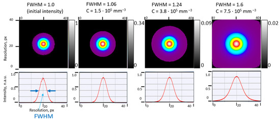
Figure 1.
Results obtained from a numerical simulation. Intensity distributions and cross-sections of laser beam propagated through the scattering medium with particular concentration values. Here, FWHM (full width at half maximum) shows the broadening of the beam due to scattering.
In order to verify our implementation of Monte Carlo technique, we compared the results of our simulation with the results obtained from “MCML” model written by Lihong Wang and Steven Jacques [8]. We considered the following parameters of simulation: half-infinite 10-mm thick layer, 1-µm diameter spheres, 1.5 × 105 mm−3 concentration value, 0.9 anisotropy factor, 0.2 mm−1 scattering coefficient, 6.8-mm initial laser beam diameter, 10 × 10-mm measurement plane size.
We used three comparison criteria:
- Number of photons transmitted through and reflected from the medium.
- Distributions of photons per scattering order (number of photons undergone 1, 2, … etc. scattering events).
- Intensity distributions at the exit edge of the medium (in Table 1, we presented percentage of photons located within specified regions).
 Table 1. Model verification: comparison of results obtained from the developed model and MCML.
Table 1 contains results of comparison of our model with MCML.
2.3. Shack–Hartmann Technique
Shack–Hartmann sensor [61,62,63,64,65,66] is well-known device that is widely used in large and diverse sets of applications, primarily to measure distortions of the wavefront of the radiation passed through different media—turbulent and/or scattering atmosphere, biological tissues, etc. Since, in our work, we consider the case of moderately scattering medium where average number of scattering events is from 0 to 10—the so-called cross-over scattering regime [67,68]—we assumed (and proved it experimentally) that the Shack–Hartmann technique still could be applied to measure the scattered laser beam distortions. We will cover this point later in Section 2.4.
In a conventional Shack–Hartmann technique, the wavefront of the incident radiation is divided into a number of sub-apertures by means of lenslet array. Lenslet array is a thin, flat base with a grid of micro lenses (lenslets) etched on the base. Each lenslet commonly has diameter from 100 to 300 µm and focal length f from 3 mm to 8 mm. Radiation passes through these lenslets and forms a set of focal spots at the measurement (sensor) plane (Figure 2a).
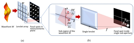
Figure 2.
(a) Set of focal spots (focal spot field, hartmannogram) formed by a lenslet array at the sensor plane of a Shack–Hartmann sensor; (b) Principle of calculation of wavefront derivatives by means of measurements of focal-spot displacement. Image adapted from [35].
Since the diameter of each lenslet is rather small, it is assumed that the wavefront W is flat within a single lenslet, and the only aberration it has is tip-tilt. In case a tip-tilt equals zero (i.e., a wavefront is flat and parallel to the plane of the lenslet), radiation is focused to the center of the corresponding sub-aperture of the sensor. In case a wavefront has non-zero tip-tilt within a lenslet, then the focal spot will be displaced (Sx, Sy) from the center of the sub-aperture proportional to the tip-tilt value (Figure 2b). In other words, if we measure these displacements Sx and Sy of the focal spot per X and Y axis, correspondingly, we will obtain the values of partial derivatives ∂W/∂x and ∂W/∂y of the wavefront W within each sub-aperture (Equation (5)):
where , —partial derivatives of the wavefront W,
f—focal spot of each lenslet,
, —displacements of a focal spot within a sub-aperture per X and Y axis.
On the other hand, in order to analytically describe and visualize the wavefront surface, one can use the polynomial approximation; for example, B-Splines [69] or Zernike polynomials [70,71,72,73], which are commonly used in optics. These polynomials are orthogonal within the unity circle and are analytically expressed in polar coordinates as follows:
Thus, the wavefront W can be presented in a form of Zernike polynomial expansion:
where —Zernike coefficient that represents the aberration value,
N—number of the Zernike polynomials used, l = n − 2m.
Knowing the analytical representation of polynomials, we can calculate the partial derivatives ∂W/∂x and ∂W/∂y of a wavefront W:
Thus, the wavefront partial derivatives ∂W/∂x and ∂W/∂y can be analytically defined using Zernike polynomials (Equation (8)). However, they can also be calculated using the measured displacements Sx and Sy of focal spots on the Shack–Hartmann sensor:
Finally, we determine the overdetermined system of linear equations with the unknown coefficients . Solving this least square problem [74], we obtain the coefficients . From here on, the wavefront can be analytically described and analyzed.
2.4. Hybrid Model Implementation
Since we implemented the simulation of a laser beam propagation through a scattering layer using Monte Carlo technique, and since we know how to estimate distortions of laser radiation using Shack–Hartmann technique, we can combine these techniques and numerically estimate what distortions (in terms of focal spots displacements) the beam will obtain after passing the scattering medium.
To solve this, we upgraded our beam propagation model by adding the implementation of Shack–Hartmann technique. In order to do so, we placed the measurements plane, as well as the plane that simulates the lenslet array, at the specified distance from the output edge of the scattering layer (this distance can be varied by the user). Since Monte Carlo technique treats the light as a huge number of photons (or photon packets), we can use the ray-tracing technique and principles of geometrical optics to calculate the trajectory of propagation of photon in free space after it leaves the scattering layer. For this, we calculate the direction cosines , , and of each photon that left the scattering layer:
where , , and —direction cosines of the photon’s propagation trajectory before it left the scattering medium (before the last photon–particle interaction).
After calculation of direction cosines, we traced the photon to the plane of the lenslet array. The photon fell on the particular lenslet that retraced it to the measurement plane according to the incidence angle. Photon’s coordinates , , were calculated using the formulas:
where —focal length of the lenslet.
As a result, we obtain a set of coordinates of all photons that fell on the lenslet array and then retraced to the measurement plane. Afterward, we discretize the measurements plane so it becomes more like the real camera sensor—with fixed pixel size and pixel resolution. The focal spot field also called hartmannogram image obtained on the 4.8 × 4.8-mm measurements plane after the simulation of 4-mm laser beam propagation through the scattering medium is presented on Figure 3.
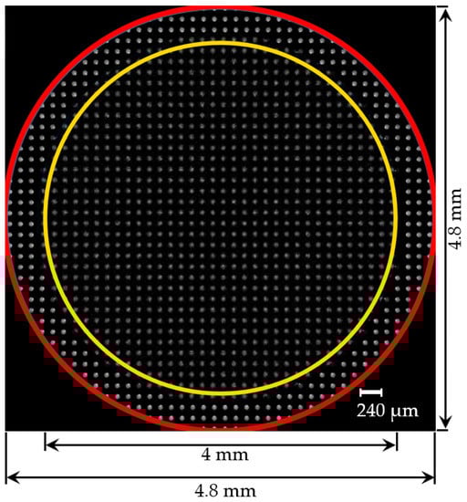
Figure 3.
Shack–Hartmann focal spot field (hartmannogram) obtained after the beam propagation through a scattering layer. The inner yellow circle corresponded to the initial diameter (4 mm) of the collimated beam before entering the scattering volume. The outer red circle corresponded to the area (4.8 mm diameter) of the Shack–Hartmann sensor where the distortions were analyzed.
It can be observed from Figure 3 that there are extra focal spots that appear out of the diameter of 4 mm (the diameter of the initial collimated laser beam that fell on the scattering layer). This effect can be explained by laser beam broadening due to light scattering. A scattered photon flux contains three components [75]: ballistic, on-axis (or “snake”); and off-axis (or diffusive) photons. Ballistic photons travel through a turbid medium without interaction with the scatterers and do not change the initial trajectory. This coherent component of the scattered light is the most important for imaging and focusing applications. On-axis photons undergo few scattering events and travel in near-forward paths along a trajectory that is close to the initial direction of the beam propagation. These photons play an important role for imaging and focusing when the thickness of the scattering medium layer increases because the number of ballistic photons decreases exponentially in this case [11]. Off-axis photons scatter in all directions and form a noncoherent component of the scattered light. As noted above, ballistic photons are most valuable for focusing, but their number decreases exponentially when the layer thickness or scatterer concentration increases. When the concentration value of the scattering medium increases, the number of on-axis and diffusive photons increases as well. In addition, all of these photons together form the extra focal spots located between yellow and red circle on Figure 3.
At this point, we could apply the Shack–Hartmann technique to estimate the distortions of scattered laser radiation. We calculated the displacements of focal spots Sx and Sy (Equation (5)) and solved the system of linear equations (Equation (9)) to find the unknown coefficients of Zernike polynomials.
During the numerical estimations, we varied the concentration value of the scattering medium from 1.3 × 10⁵ to 106 mm−3. We simulated the propagation of the photon flux through the scattering medium with eight particular concentration values from this range. Figure 4 shows some of hartmannogram images obtained on Shack–Hartmann during simulation of laser beam propagation through a scattering medium with different concentrations.
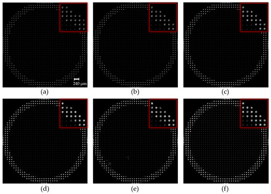
Figure 4.
Hartmannogram images obtained from the simulation of laser beam propagation through a scattering medium with different concentration values: (a) 1.3 × 105 mm−3, (b) 4.4 × 105 mm−3, (c) 7.4 × 105 mm−3, (d) 9.4 × 105 mm−3, (e) 106 mm−3, and (f) 1.2 × 106 mm−3. The enlarged region of top-right corner of each hartmannogram is depicted in red squares.
It can be observed that the spots within the initial aperture of the beam that equaled 4 mm are presented as delta functions centered in the center of the corresponding sub-apertures—this is because the number of ballistic photons is much bigger than the others. The peripheral focal spots outside of the initial diameter are much wider in diameter, but they also have the clear-cut center. This is due to the impact of rather big portion of on-axis photons (Figure 4a–c). However, with the increase of the concentration of scatterers, the intensity distribution within each peripheral focal spot became uneven without the strongly marked center (Figure 4d–f). This is due to the impact of diffusive photons.
As is known, conventional Shack–Hartmann sensor allows for the measurement of the wavefront of radiation. However, when a laser beam passes through a scattering medium, it does not have the wavefront in strict physical sense since part of the radiation is scattered. Figure 5 explains what we actually measure with a Shack–Hartmann sensor in this work.
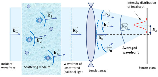
Figure 5.
Explanation of the term “averaged wavefront”.
Initially, before the scattering medium, the beam has a flat-incident wavefront. The scatterers with which radiation interacts become point sources of secondary spherical waves with their own wave vectors . At the same time, part of the radiation passes through the medium without scattering (so-called ballistic component), retaining the original flat wavefront. As a result, a focal spot is formed at the focal plane of the lenslet. In addition, the displacement of this focal spot from the optical axis of the lenslet is proportional to the local slope of a so-called “average wavefront”, which is composed of a set of, generally speaking, independent wavefronts corresponding to different point sources (i.e., scatterers in the medium). Moreover, we measure and analyze this average wavefront.
Due to the axial symmetry nature of the Mie scattering process, only symmetrical distortions of the average wavefront were obtained in the simulation. The obtained coefficients of symmetrical Zernike polynomials (#3, #8, #15, #24) are presented on Figure 6.
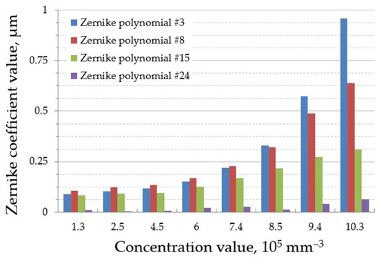
Figure 6.
Symmetrical Zernike coefficient dependence on the concentration value of scattering medium.
It can be clearly seen from Figure 6 that the amplitude of distortions (values of Zernike coefficients) increased with the increase of the scatterers’ concentration. The reason for that is explained by the decrease of ballistic photons and, at the same time, the increase of non-ballistic photons. Finally, it led to the displacements of the focal spot centers from its reference positions.
3. Hybrid Model Verification: Experimental Results and Discussion
In order to verify the developed hybrid model of the estimation of distortions of a laser beam that passed through a scattering layer, we assembled the experimental setup. The photo of the laboratory setup is presented in Figure 7.
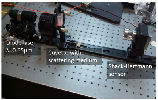
Figure 7.
Photo of the experimental setup with a diode laser and a Shack–Hartmann sensor.
Laser radiation comes from the fiber-coupled diode laser and propagates through the collimator. The collimated laser beam of 4 mm in diameter then passes through the transparent glass cuvette with the thickness of 5 mm and dimensions of 18 × 18 mm, filled with the scattering suspension of 1 µm-diameter polystyrene microbeads produced by Magsphere, Inc. (Pasadena, CA, USA) [76] with the refractive index equaled to 1.582 [52] diluted in distilled water (refractive index is 1.33). The beam resulting from the cuvette is registered on the Shack–Hartmann sensor [77]. According to the specification sheet on the polystyrene microbeads, the diameter variation was within 10%. The microbeads have a smooth surface [78] so that no complicated shape-scattering diagram from a single microbead is produced. Shack–Hartmann sensor consisted of a digital CCD camera Basler A302fs (1/2-inch sensor with the size of the receiving area equaled to 6.4 × 4.8 mm, camera frame rate is 30 Hz) and a lenslet array (focal length—6 mm, diameter of a lenslet—150 µm, total number of lenslets—greater than 1300). The distance between the Shack–Hartmann sensor and the cuvette was set to 450 mm in order to decrease the impact of the totally diffused photons on the quality of the measurements. Since we made the experiments in a very short period after the preparation of the suspension of scattering particles, the concentration during the experimental measurements was not varied; or, at least, its variation has no impact on the measurements. Moreover, for all of our measurements, we averaged hartmannograms in order to increase the accuracy. For each experiment, we prepared the new suspension. If the cuvette with the initial high-concentration solution was not used for a long period of time, we used the ultrasonic bath to split the coagulated microbeads.
We analyze the average wavefront of scattered light in the circular aperture of 4.8 mm. The aperture’s center and the cameras’ center coincide. The initial laser beam diameter was 4 mm, whereas the aperture diameter was 4.8 mm. It was necessary to analyze how the non-ballistic photons impact on the distortions of scattered light. The average wavefront measured by the Shack–Hartmann sensor was approximated by Zernike polynomials, as it was done in the simulation.
Figure 8 shows the comparison of the dependence of distortion amplitude (amplitude of distortions of the averaged wavefront) on the concentration values of scatterers. Both the model and experimental curves demonstrated similar trends of increasing the amplitude of distortions while increasing the concentration values of the scatterers.
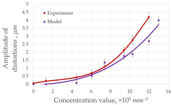
Figure 8.
Trend lines of the dependence of the amplitude of distortions on the concentration values for the simulation (red curve) and for the experiment (purple curve). Image adapted from [37].
Figure 8 shows a similar trend of increasing distortions of the average wavefront of the scattered laser beam with increasing concentrations of scatterers in the medium in the range from 105 to 106 mm−3, both for the model and laboratory experiment. There are a few reasons why the model curve differs from the experimental one. The explanation is schematically represented on Figure 9.
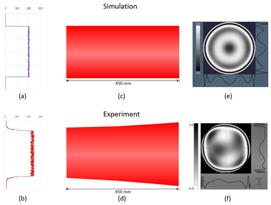
Figure 9.
Initial intensity distribution of the simulated (a) and real, experimental (b) laser beam; schematical representation of laser beam propagation without diffraction (c) and with diffraction (d); reconstructed interference pattern with symmetrical distortions only (e) obtained in the simulation and with both symmetrical and non-symmetrical distortions (f) obtained in the real experiment.
First, in the model (Figure 9a), we did not reproduce the initial distribution of the intensity of the real laser source used in the experiment (Figure 9b). In fact, a generator of uniformly distributed random numbers is used to generate the initial distribution of photons in the model. Second, the model does not take into account a diffraction phenomenon (Figure 9c), which takes place when the real laser beam is propagating through the optical path (Figure 9d). In the experiment, as a result of diffraction, the focal spots on the Shack–Hartmann sensor in the central part of the beam are displaced from the centers of corresponding sub-apertures at high scatterer concentrations, which leads to additional defocusing. This effect was not observed in the model. For this reason, the experimental curve on Figure 8 increases faster than the model curve at high concentrations. Third, in addition to the centrally symmetric aberrations in the average wavefront, there were also other distortions (in particular, coma aberration) in the experiment (Figure 9f), which could not exist in the model (Figure 9e) in principle due to the symmetry of the nature of Mie scattering on spherical particles. This was due to the fact that the walls of the glass cuvette were not plane-parallel. We have also examined this problem in detail; the results can be found in [79]. We made the measurements and determined that the cuvette walls were not absolutely parallel. The deviation was not huge, but in conjugation with the impact of the scattering medium, it led to an overall tilt and, finally, coma aberration. Thus, an additional slope was introduced into the laser beam and, as a result, the coma aberration.
It can be observed from Figure 8 that there is one more data point in the model curve (for a concentration of the order of 106 mm−3). This is due to the fact that when a laser beam propagates through a scattering medium with a particles’ concentration of the order of 106 mm−3, only fractions of a percent of the initial radiation energy level reach the sensor aperture. The traditional, most popular, and widespread CCD cameras have insufficient quantum efficiency and a limited exposure range to detect radiation of such a low power. Regarding the numerical simulation, we could use any concentration values, since with a statistically sufficient number of simulated photons, it is possible to obtain an image of focal spot field. We displayed this data point to show that the model curve does not move far away from the experimental curve even with an increase in the concentration of scatterers.
Thus, the data obtained in the developed model and, subsequently, in a laboratory experiment showed that with an increase in the concentration of scattering particles in the range from 105 to 106 mm−3, the amplitude of distortions of the average wavefront of radiation propagating through the layer of the scattering medium increases.
4. Conclusions
In this paper, we presented the numerical model and algorithm of measurements of distortions of the laser beam that passed through a moderately scattering medium. The simulation of beam propagation through a scattering medium was implemented using the Monte Carlo simulation, the scattered beam propagation in free space from the edge of scattering medium to the lenslet array of the Shack–Hartmann sensor was implemented using ray-tracing techniques, and the measurements of beam distortions was implemented using the Shack–Hartmann technique. We measured the amplitude of distortions of the scattered beam by estimating the displacements of focal spots on the Shack–Hartmann sensor. Both the model and experiment demonstrated similar trends of exponential increase of the amplitude of distortions with the increase of concentration values of the scattering particles in the medium.
Author Contributions
Conceptualization, I.G., A.N. and A.K.; methodology, I.G. and A.N.; software, I.G.; validation, I.G.; formal analysis, A.K.; investigation, I.G.; resources, I.G. and V.T.; data curation, A.K.; writing—original draft preparation, I.G.; writing—review and editing, I.G., J.S. and V.T.; visualization, I.G.; supervision, J.S.; project administration, A.K.; funding acquisition, J.S. All authors have read and agreed to the published version of the manuscript.
Funding
This research was funded by the Russian Science Foundation, Grant No. 20-19-00597.
Data Availability Statement
The part of the data presented in this study is obtained using the developed software that are openly available in https://github.com/burning-daylight/Visscat (accessed on 5 July 2023).
Conflicts of Interest
The authors declare no conflict of interest.
References
- Berrocal, E.; Sedarsky, D.; Paciaroni, M.; Meglinski, I.; Linne, M. Laser light scattering in turbid media Part I: Experimental and simulated results for the spatial intensity distribution. Opt. Express 2007, 15, 10649–10665. [Google Scholar] [CrossRef] [PubMed]
- Measures, R.M. Laser Remote Sensing: Fundamentals and Applications; Krieger: Malabar, FL, USA, 1992. [Google Scholar]
- Shao, B.; Jaffe, J.S.; Chachisvilis, M.; Esener, S.C. Angular resolved light scattering for discriminating among marine picoplankton: Modeling and experimental measurements. Opt. Express 2006, 14, 12473–12484. [Google Scholar] [CrossRef] [PubMed]
- Tuchin, V.V. Handbook of Optical Biomedical Diagnostics; SPIE Press: Bellingham, WA, USA, 2002. [Google Scholar]
- Lee, C.-K.; Sun, C.-W.; Lee, P.-L.; Lee, H.-C.; Yang, C.; Jiang, C.-P.; Tong, Y.-P.; Yeh, T.-C.; Hsieh, J.-C. Study of photon migration with various source-detector separations in near-infrared spectroscopic brain imaging based on three-dimensional Monte Carlo modeling. Opt. Express 2005, 13, 8339–8348. [Google Scholar] [CrossRef]
- Berrocal, E. Multiple Scattering of Light in Optical Diagnostics of Dense Sprays and Other Complex Turbid Media. Ph.D. Thesis, Cranfield University, Cranfield, UK, 2006. [Google Scholar]
- Sobol, I. The Monte Carlo Method; The University of Chicago Press: Chicago, IL, USA, 1974. [Google Scholar]
- Wang, L.; Jacques, S.L.; Zheng, L. MCML—Monte Carlo modelling of light transport in multi-layered tissues. Comput. Methods Programs Biomed. 1995, 47, 131–146. [Google Scholar] [CrossRef]
- Churmakov, D.Y. Multipurpose Computational Model for Modern Optical Diagnostics and Its Biomedical Applications. Ph.D. Thesis, Cranfield University, Cranfield, UK, 2005. [Google Scholar]
- Boas, D.; Culver, J.; Stott, J.; Dunn, A. Three dimensional Monte Carlo code for photon migration through complex heterogeneous media including the adult human head. Opt. Express 2002, 10, 159–170. [Google Scholar] [CrossRef] [PubMed]
- Mosk, A.P.; Lagendijk, A.; Lerosey, G.; Fink, M. Controlling waves in space and time for imaging and focusing in complex media. Nat. Photonics 2012, 6, 283. [Google Scholar] [CrossRef]
- Bashkatov, A.N.; Priezzhev, A.V.; Tuchin, V.V. Laser technologies in biophotonics. Quantum Electron. 2012, 42, 379. [Google Scholar] [CrossRef]
- Vellekoop, I.M.; Mosk, A.P. Focusing coherent light through opaque strongly scattering media. Opt. Lett. 2007, 32, 2309. [Google Scholar] [CrossRef]
- Zhang, Y.; Chen, Y.; Yu, Y.; Xue, X.; Tuchin, V.V.; Zhu, D. Visible and near-infrared spectroscopy for distinguishing malignant tumor tissue from benign tumor and normal breast tissues in vitro. J. Biomed. Opt. 2013, 18, 077003. [Google Scholar] [CrossRef]
- Goodman, J.W.; Huntley, W.H., Jr.; Jackson, D.W.; Lehmann, M. Wavefront reconstruction imaging through random media. Appl. Phys. Lett. 1966, 8, 311–313. [Google Scholar] [CrossRef]
- Kogelnik, H.; Pennington, K.S. Holographic imaging through a random medium. J. Opt. Soc. Am. 1968, 58, 273–274. [Google Scholar] [CrossRef]
- Matthews, T.; Medina, M.; Maher, J.; Levinson, H.; Brown, W.; Wax, A. Deep tissue imaging using spectroscopic analysis of multiply scattered light. Optica 2014, 1, 105. [Google Scholar] [CrossRef]
- Bertolotti, J.; van Putten, E.G.; Blum, C.; Lagendijk, A.; Vos, W.L.; Mosk, A.P. Non-invasive imaging through opaque scattering layers. Nature 2012, 491, 232–234. [Google Scholar] [CrossRef]
- Katz, O.; Small, E.; Silberberg, Y. Looking around corners and through thin turbid layers in real time with scattered incoherent light. Nat. Photon. 2012, 6, 549–553. [Google Scholar] [CrossRef]
- Popoff, S.M.; Lerosey, G.; Carminati, R.; Fink, M.; Boccara, A.C.; Gigan, S. Measuring the transmission matrix in optics: An approach to the study and control of light propagation in disordered media. Phys. Rev. Lett. 2010, 104, 100601. [Google Scholar] [CrossRef]
- Conkey, D.B.; Caravaca-Aguirre, A.M.; Piestun, R. High-speed scattering medium characterization with application to focusing light through turbid media. Opt. Express 2012, 20, 1733–1740. [Google Scholar] [CrossRef] [PubMed]
- Hsieh, C.; Pu, Y.; Grange, R.; Laporte, G.; Psaltis, D. Imaging through turbid layers by scanning the phase conjugated second harmonic radiation from a nanoparticle. Opt. Express 2010, 18, 20723–20731. [Google Scholar] [CrossRef]
- Stockbridge, C.; Lu, Y.; Moore, J.; Hoffman, S.; Paxman, R.; Toussaint, K.; Bifano, T. Focusing through dynamic scattering media. Opt. Express 2012, 20, 15086–15092. [Google Scholar] [CrossRef]
- Xu, J.; Ruan, H.; Liu, Y.; Zhou, H.; Yang, C. Focusing light through scattering media by transmission matrix inversion. Opt. Express 2017, 25, 27234–27246. [Google Scholar] [CrossRef]
- Zhou, E.H.; Ruan, H.; Yang, C.; Judkewitz, B. Focusing on moving targets through scattering samples. Optica 2014, 1, 227–232. [Google Scholar] [CrossRef]
- Shen, Y.; Liu, Y.; Ma, C.; Wang, L.V. Focusing light through scattering media by full-polarization digital optical phase conjugation. Opt. Lett. 2016, 41, 1130–1133. [Google Scholar] [CrossRef] [PubMed]
- Feldkhun, D.; Tzang, O.; Wagner, K.H.; Piestun, R. Focusing and scanning through scattering media in microseconds. Optica 2019, 6, 72–75. [Google Scholar] [CrossRef]
- Galaktionov, I.; Kudryashov, A.; Sheldakova, J.; Nikitin, A. Laser beam focusing through the scattering medium using bimorph deformable mirror and spatial light modulator. Proc. SPIE 2019, 11135, 111350B. [Google Scholar]
- Galaktionov, I.; Sheldakova, J.; Kudryashov, A. Scattered laser beam control using bimorph deformable mirror. In Proceedings of the 18th International Conference “Laser Optics 2018”, St. Petersburg, Russia, 5–7 June 2018; p. 186. [Google Scholar]
- Galaktionov, I.; Sheldakova, J.; Toporovsky, V.; Samarkin, V.; Kudryashov, A. Bimorph vs stacked actuator deformable mirror for laser beam focusing through a moderately scattering medium. Proc. SPIE 2021, 11672, 1167214. [Google Scholar]
- Belousov, V.N.; Galaktionov, I.V.; Kudryashov, A.V.; Nikitin, A.N.; Otrubyannikova, O.V.; Rukosuev, A.L.; Samarkin, V.V.; Sivertceva, I.V.; Sheldakova, J.V. Adaptive optical system for correction of laser beam going through turbulent atmosphere. Proc. SPIE 2020, 11560, 1156026. [Google Scholar]
- Rukosuev, A.; Belousov, V.; Galaktionov, I.; Kudryashov, A.; Nikitin, A.; Samarkin, V.; Sheldakova, J. 1.5 kHz adaptive optical system for free-space communication tasks. Proc. SPIE 2020, 11272, 112721G. [Google Scholar]
- Nikitin, A.; Galaktionov, I.; Sheldakova, J.; Kudryashov, A.; Samarkin, V.; Rukosuev, A. Focusing laser beam through pinhole using bimorph deformable mirror. Proc. SPIE 2019, 10904, 109041I. [Google Scholar]
- Li, R.; Jin, D.; Pan, D.; Ji, S.; Xin, C.; Liu, G.; Fan, S.; Wu, H.; Li, J.; Hu, Y.; et al. Stimuli-Responsive Actuator Fabricated by Dynamic Asymmetric Femtosecond Bessel Beam for In Situ Particle and Cell Manipulation. ACS Nano 2020, 14, 5233–5242. [Google Scholar] [CrossRef]
- Galaktionov, I.; Nikitin, A.; Sheldakova, J.; Toporovsky, V.; Kudryashov, A. Focusing of a Laser Beam Passed through a Moderately Scattering Medium Using Phase-Only Spatial Light Modulator. Photonics 2022, 9, 296. [Google Scholar] [CrossRef]
- Sheldakova, J.; Toporovsky, V.; Galaktionov, I.; Nikitin, A.; Rukosuev, A.; Samarkin, V.; Kudryashov, A. Flat-top beam formation with miniature bimorph deformable mirror. Proc. SPIE 2020, 11486, 114860E. [Google Scholar]
- Galaktionov, I.; Sheldakova, J.; Nikitin, A.; Samarkin, V.; Parfenov, V.; Kudryashov, A. Laser beam focusing through a moderately scattering medium using a bimorph mirror. Opt. Express 2020, 28, 38061–38075. [Google Scholar] [CrossRef] [PubMed]
- Durant, S.; Calvo-Perez, O.; Vukadinovic, N.; Greffet, J.-J. Light scattering by a random distribution of particles embedded in absorbing media: Full-wave Monte Carlo solutions of the extinction coefficient. J. Opt. Soc. Am. A 2007, 24, 2953–2962. [Google Scholar] [CrossRef]
- Lacasa, J.; Hefley, T.J.; Otegui, M.E.; Ciampitti, I.A. A practical guide to estimating the light extinction coefficient with nonlinear models—A case study on maize. Plant Methods 2021, 17, 60. [Google Scholar] [CrossRef]
- Scattering Coefficient Definition. Available online: https://omlc.org/classroom/ece532/class3/musdefinition.html (accessed on 19 June 2023).
- Hohmann, M.; Lengenfelder, B.; Muhr, D.; Späth, M.; Hauptkorn, M.; Klämpfl, F.; Schmidt, M. Direct measurement of the scattering coefficient. Biomed. Opt. Express 2021, 12, 320–335. [Google Scholar] [CrossRef] [PubMed]
- Hsia, Y.; Fang, N.; Widatallah, H.; Wu, D.M.; Lee, X.M.; Zhang, J.R. Brownian motion of suspended particles in an anisotropic medium. Hyperfine Interact. 2000, 126, 401–406. [Google Scholar] [CrossRef]
- Vorob’eva, E.A.; Gurov, I.P. Models of Propagation and Scattering of Optical Radiation in Randomly Inhomogeneous Media; Meditsina: Moscow, Russia, 2006.
- Zege, E.P.; Ivanov, A.P.; Katsev, I.L. Image Transfer through a Scattering Medium; Springer: New York, NY, USA; Berlin/Heidelberg, Germany, 1991; p. 131. [Google Scholar]
- Jacques, S.L.; Prahl, S.A. Henyey-Greenstein Scattering Function. Available online: http://omlc.org/classroom/ece532/class3/hg.html (accessed on 7 June 2023).
- Wilson, B.C.; Adam, G. A Monte Carlo model for the absorption and flux distributions of light in tissue. Med. Phys. 1983, 10, 824–830. [Google Scholar] [CrossRef]
- Keijzer, M.; Jacques, S.L.; Prahl, S.A.; Welch, A.J. Light distributions in artery tissue: Monte Carlo simulations for finite-diameter laser beams. Lasers Surg. Med. 1989, 9, 148–154. [Google Scholar] [CrossRef]
- Prahl, S.A.; Keijzer, M.; Jacques, S.L.; Welch, A.J. A Monte Carlo model of light propagation in tissue. In Dosimetry of Laser Radiation in Medicine and Biology; SPIE Series; Muller, G., Sliney, D., Eds.; SPIE: Bellingham, WA, USA, 1989; pp. 102–111. [Google Scholar]
- Meglinski, I.V. Quantitative assessment of skin layers absorption and skin reflectance spectra simulation in the visible and near-infrared spectral regions. Physiol. Meas. 2002, 23, 741. [Google Scholar] [CrossRef]
- Kandidov, V.; Militsin, V.; Bykov, A.; Priezzhev, A. Application of corpuscular and wave Monte-Carlo methods in optics of dispersive media. Quantum Electron. 2006, 36, 1003. [Google Scholar] [CrossRef]
- Han, X.; Shen, J.; Yin, P.; Hu, S.; Bi, D. Influences of refractive index on forward light scattering. Opt. Commun. 2014, 316, 198–205. [Google Scholar] [CrossRef]
- Ma, X.; Lu, J.; Brocks, S.; Jacob, K.; Yang, P.; Xin, X.-H. Determination of complex refractive index of polystyrene microspheres from 370 to 1610 nm. Phys. Med. Biol. 2003, 48, 4165. [Google Scholar] [CrossRef]
- Piskozub, J.; McKee, D. Effective scattering phase functions for the multiple scattering regime. Opt. Express 2011, 19, 4786–4794. [Google Scholar] [CrossRef] [PubMed]
- Mishchenko, M.; Travis, L.D.; Lacis, A.A. Multiple Scattering of Light by Particles: Radiative Transfer and Coherent Backscattering; Cambridge University Press: Cambridge, UK, 2006. [Google Scholar]
- Zvereva, S. In the world of sunlight. Hydrometizdat 1988, 160. [Google Scholar]
- Fukutomi, D.; Ishii, K.; Awazu, K. Determination of the scattering coefficient of biological tissue considering the wavelength and absorption dependence of the anisotropy factor. Opt. Rev. 2016, 23, 291–298. [Google Scholar] [CrossRef]
- Lobanova, M.A.; Vasiliev, A.V.; Melnikova, I.N. Dependence of anisotropy factor of scattering phase function on the medium parameters. Mod. Probl. Remote Sens. Earth Space 2010, 7. [Google Scholar]
- Bashkatov, A.; Genina, E.; Tuchin, V.; Altshuler, G.; Yaroslavsky, I. Monte Carlo study of skin optical clearing to enhance light penetration in the tissue: Implications for photodynamic therapy of acne vulgaris. Proc. SPIE 2008, 7022, 702209. [Google Scholar]
- Vitkin, E.; Turzhitsky, V.; Qiu, L.; Guo, L.; Itzkan, I.; Hanlon, E.B.; Perelman, L.T. Photon diffusion near the point-of-entry in anisotropically scattering turbid media. Nat. Commun. 2011, 2, 587. [Google Scholar] [CrossRef]
- Tschukin, O.; Silberzahn, A.; Selzer, M.; Amos, P.G.K.; Schneider, D.; Nestler, B. Concepts of modeling surface energy anisotropy in phase-field approaches. Geotherm Energy 2017, 5, 19. [Google Scholar] [CrossRef]
- Platt, B.; Shack, R.J. History and principles of Shack-Hartmann wavefront sensing. Refr. Surg. 2001, 17, 15. [Google Scholar] [CrossRef] [PubMed]
- Liang, J.; Grimm, B.; Goelz, S.; Bille, J.F. Objective measurement of the wave aberrations of the human eye with the use of a Hartmann-Shack wave-front sensor. J. Opt. Soc. Am. A 1994, 11, 1949. [Google Scholar] [CrossRef]
- Lane, R.G. Wave-front reconstruction using a Shack–Hartmann sensor. Appl. Opt. 1992, 31, 6902. [Google Scholar] [CrossRef] [PubMed]
- Primot, J. Theoretical description of Shack–Hartmann wave-front sensor. Opt. Commun. 2003, 222, 81–92. [Google Scholar] [CrossRef]
- Konnik, M.; Doná, J. Waffle mode mitigation in adaptive optics systems: A constrained Receding Horizon Control approach. In Proceedings of the American Control Conference, Washington, DC, USA, 17–19 June 2013; pp. 3390–3396. [Google Scholar]
- Mauch, S.; Reger, J. Real-Time Spot Detection and Ordering for a Shack–Hartmann Wavefront Sensor With a Low-Cost FPGA. Proc. IEEE Trans. Instrum. Meas. 2014, 63, 2379–2386. [Google Scholar] [CrossRef]
- Vellekoop, I. Feedback-based wavefront shaping. Opt. Express 2015, 23, 12189–12206. [Google Scholar] [CrossRef]
- Galaktionov, I.V. Increase of Focusing Efficiency of Scattered Laser Radiation by Means of Adaptive Optics. Ph.D. Thesis, Institute of Applied Physics Russian Academy of Sciences, Nizhniy Novgorod, Russia, 2021. [Google Scholar]
- Galaktionov, I.; Nikitin, A.; Sheldakova, J.; Kudryashov, A. B-spline approximation of a wavefront measured by Shack-Hartmann sensor. Proc. SPIE 2021, 11818, 118180N. [Google Scholar]
- Malacara-Hernandez, D. Wavefront fitting with discrete orthogonal polynomials in a unit radius circle. Opt. Eng. 1990, 29. [Google Scholar] [CrossRef]
- Wyant, J.C.; Creath, K. Basic wavefront aberration theory for optical metrology. In Proceedings of Applied Optics and Optical Engineering; Academic Press, Inc.: Cambridge, MA, USA, 1992; pp. 27–39. [Google Scholar]
- Genberg, V.; Michels, G.; Doyle, K. Orthogonality of Zernike polynomials. Proc. SPIE 2002, 4771. [Google Scholar] [CrossRef]
- Lakshminarayanan, V.; Fleck, A. Zernike polynomials: A guide. J. Mod. Opt. 2011, 58, 545–561. [Google Scholar] [CrossRef]
- Linnik, J.V. Least Square Error Method and the Basics of Mathematical-Statistical Theory, 2nd ed.; Mir Publishers: Moscow, Russia, 1962. [Google Scholar]
- Ramachandran, H. Imaging through turbid media. Curr. Sci. 1999, 76, 1334. [Google Scholar]
- Polystyrene Microbeads. Available online: https://magsphere.com/Products/Polystyrene-Latex-Particles/polystyrene-latex-particles.html (accessed on 19 June 2023).
- Galaktionov, I.; Sheldakova, J.; Kudryashov, A. Laser beam focusing through the scattering medium using 14-, 32- and 48-channel bimorph mirrors. In Proceedings of the 18th International Conference “Laser Optics 2018”, St. Petersburg, Russia, 5–7 June 2018; p. 223. [Google Scholar]
- Liu, Y.; Hu, J. Investigation of Polystyrene-Based Microspheres from Different Copolymers and Their Structural Color Coatings on Wood Surface. Coatings 2021, 11, 14. [Google Scholar] [CrossRef]
- Galaktionov, I.V.; Kudryashov, A.V.; Sheldakova, J.V.; Byalko, A.A.; Borsoni, G. Measurement and correction of the wavefront of the laser light in a turbid medium. Quantum Electron. 2017, 47, 32–37. [Google Scholar] [CrossRef]
Disclaimer/Publisher’s Note: The statements, opinions and data contained in all publications are solely those of the individual author(s) and contributor(s) and not of MDPI and/or the editor(s). MDPI and/or the editor(s) disclaim responsibility for any injury to people or property resulting from any ideas, methods, instructions or products referred to in the content. |
© 2023 by the authors. Licensee MDPI, Basel, Switzerland. This article is an open access article distributed under the terms and conditions of the Creative Commons Attribution (CC BY) license (https://creativecommons.org/licenses/by/4.0/).