ω-Circulant Matrices: A Selection of Modern Applications from Preconditioning of Approximated PDEs to Subdivision Schemes

Abstract

It is well known that $\omega$-circulant matrices with $\omega \ne 0$ can be simultaneously diagonalized by a transform matrix, which can be factored as the product of a diagonal matrix, depending on $\omega$, and of the unitary matrix $F_n$ associated to the Fast Fourier Transform. Hence, all the sets of $\omega$-circulants form algebras whose computational power, in terms of complexity, is the same as the classical circulants with $\omega =1$. However, stability is a delicate issue, since the condition number of the transform is equal to that of the diagonal part, tending to $\max \left\{\right|\omega |,|\omega {|}^{-1}\}$. For $\omega =0$, the set of related matrices is still an algebra, which is the algebra of lower triangular matrices, but they do not admit a common transform since most of them (all except the multiples of the identity) are non-diagonalizable. In the present work, we review two modern applications, ranging from parallel computing in preconditioning of PDE approximations to algorithms for subdivision schemes, and we emphasize the role of such algebra. For the two problems, few numerical tests are conducted and critically discussed and the related conclusions are drawn.

1. Introduction

When dealing with structured matrices of Toeplitz type [1,2] not related to fast trigonometric transforms, the problems of computing the solution of large linear system, the matrix vector product, or the eigenvalues are greatly accelerated by using them as approximation matrices belonging to algebras associated to trigonometric transforms [3,4,5,6]. Among them, a very classical choice is the algebra of $\omega$-circulant matrices with $\omega \ne 0$ (see the seminal book [7] and references therein). In this work, after briefly introducing these matrices and reviewing a few related applications, we focus on new, challenging problems, such as parallel computing in preconditioning of approximated partial differential equations (PDEs) and algorithms for subdivision schemes, highlighting the benefits and drawbacks of employing $\omega$-circulant matrices.

The paper is organized in the following manner. In Section 2 we introduce the basic notions on circulant and $\omega$-circulant matrices. In Section 3, after recalling a technique for the parallel computing of the matrix-vector product and matrix inversion concerning $\omega$-circulant matrices, we present a general procedure (introduced by Bini [8]) to precondition (block) triangular Toeplitz linear systems. Then, we move on to scalar subdivision schemes, introducing them in Section 4 and presenting the interpolation model as a direct problem with its associated inverse problem in Section 5. Section 6 is devoted to selected numerical experiments and the related critical discussion. To conclude, in Section 7 we draw conclusions and discuss a few open problems, with special attention to the use of structured matrices in subdivision schemes.

2. Some Remarks on Circulant and $\mathit{\omega }$-Circulant Matrices

In this introductory section, we lay the groundwork for the main part of this paper by recalling the basic definitions and properties of both circulant and $\omega$-circulant matrices. More information can be found in Ref. [7]. We recall that circulant and $\omega$-circulant matrices have played a major role in the last four decades for the fast solution of structured linear systems, mainly of Toeplitz type, but also stemming from approximated PDEs. Classical references are Refs. [2,9,10,11,12,13,14], where preconditioned Krylov methods, local Fourier analysis, and its GLT generalizations are treated with attention to the circulant structure and to the related fast Fourier transform (FFT); see Ref. [15]. More specific references for the numerical treatment of PDEs via $\omega$-circulant preconditioning or directly by multigrid solvers or combination of them can be found in Refs. [10,16,17,18].

Definition 1.

Consider $\mathit{\alpha }=[{\alpha }_0,{\alpha }_1,\dots ,{\alpha }_{n-1}]$ with ${\alpha }_j\in \mathbb{R}$. A square matrix $\mathbf{C}\in {\mathbb{R}}^{n\times n}$is called circulant and it is denoted with $\mathbf{C}=circ\left(\mathit{\alpha }\right)$ if we have

$${\left(\mathbf{C}\right)}_{s,t}={\alpha }_{s-t(modn)}\forall s,t=0,\dots ,n-1.$$

An equivalent and compact representation of $\mathbf{C}$ is given by

$$\mathbf{C}=\sum _{j=0}^{n-1}{\Pi }_n^j{\alpha }_j,$$

where ${\Pi }_n$ is the permutation matrix

$${\Pi }_n=\left[\begin{array}{cccccc}0& 0& 0& \dots & 0& 1\\ 1& 0& 0& \dots & 0& 0\\ 0& 1& 0& \dots & 0& 0\\ 0& 0& 1& \dots & 0& 0\\ \ddots & \ddots & \ddots & \ddots & \ddots & \ddots \\ 0& 0& 0& \dots & 1& 0\end{array}\right].$$

Note that for any fixed $p,q\in \mathbb{N}$ the matrix ${\displaystyle \mathbf{C}=\sum _{j=-p}^q{\Pi }_n^j{\alpha }_j}$ is circulant, since this sum can always be traced back to the form in the above definition.

Denoting with ${·}^{*}$ the conjugate transpose, circulant matrices admit the following spectral decomposition.

Proposition 1.

$\mathbf{C}$ can be diagonalized as

$$\mathbf{C}=F_n{L}_n{F}_n^{*},$$

where

$$L_n={\mathrm{diag}}_{s=0,\dots ,n-1}\left(\sum _{j=0}^{n-1}exp\left(2\pi \mathrm{i}\frac{sj}{n}\right){\alpha }_j\right)$$

is the diagonal matrix containing the eigenvalues of $\mathbf{C}$ and

$$F_n={\frac{1}{\sqrt{n}}\left[\begin{array}{c}exp\left(-2\pi \mathrm{i}\frac{jk}{n}\right)\end{array}\right]}_{j,k=0}^{n-1},{\mathrm{i}}^2=-1$$

is the unitary Fourier matrix.

Proof. 

By a direct computation of the eigenvalues, it is easy to verify that ${\Pi }_n$ factorizes as

$${\Pi }_n=F_n{\Omega }_n{F}_n^{*}$$

(1)

with

$${\Omega }_n={\mathrm{diag}}_{s=0,\dots ,n-1}\left(\exp \left(2\pi \mathrm{i}\frac{s}{n}\right)\right).$$

(2)

The thesis follows. □

Remark 1.

The eigenvalues of $\mathbf{C}$, namely the diagonal elements of $L_n$, are given by the Fourier transform of the first column of $\mathbf{C}$. Alternatively, they can be seen as

$$\Lambda \left(\mathbf{C}\right)=\left\{f\left(\frac{2\pi s}{n}\right),s=0,\dots ,n-1\right\},$$

where the function ${\displaystyle f\left(\theta \right):=\sum _{j=0}^{n-1}{\alpha }_{j}exp\left(\mathrm{i}j\theta \right)}$is called (spectral) symbol of $\mathbf{C}$.

$\omega$-circulant matrices represent an extension of the notion of circulant matrix (see, e.g., Refs. [6,19,20] for more details).

Definition 2.

Consider $\mathit{\alpha }=[{\alpha }_0,{\alpha }_1,\dots ,{\alpha }_{n-1}]$ with ${\alpha }_j\in \mathbb{R}$. A square matrix ${\mathbf{C}}_{\omega }\in {\mathbb{R}}^{n\times n}$ is called$\omega$-circulant and it is denoted with ${\mathbf{C}}_{\omega }={circ}_{\omega }\left(\mathit{\alpha }\right)$if it holds

$${\left({\mathbf{C}}_{\omega }\right)}_{s,t}=\left\{\begin{array}{cc}{\alpha }_{s-t(modn)},\hfill & ifs>t,\hfill \\ \omega {\alpha }_{s-t(modn)},\hfill & ifs\le t,\hfill \end{array}\right.\forall s,t=0,\dots ,n-1.$$

A compact representation for ${\mathbf{C}}_{\omega }$ is given by

$${\mathbf{C}}_{\omega }=\sum _{j=0}^{n-1}{\Pi }_{n,\omega }^j{\alpha }_j,$$

where ${\Pi }_{n,\omega }$ is the matrix

$${\Pi }_{n,\omega }=\left[\begin{array}{cccccc}0& 0& 0& \dots & 0& \omega \\ 1& 0& 0& \dots & 0& 0\\ 0& 1& 0& \dots & 0& 0\\ 0& 0& 1& \dots & 0& 0\\ \ddots & \ddots & \ddots & \ddots & \ddots & \ddots \\ 0& 0& 0& \dots & 1& 0\end{array}\right].$$

Note that setting $\omega =1$ leads back to Definition 1. An analogous spectral decomposition can be derived.

Proposition 2.

${\mathbf{C}}_{\omega }$ can be diagonalized as

$${\mathbf{C}}_{\omega }=F_{n,\omega }{L}_{n,\omega }{F}_{n,\omega }^{-1},$$

where

$$L_{n,\omega }={\mathrm{diag}}_{s=0,\dots ,n-1}\left(\sum _{j=0}^{n-1}{\omega }^{j/n}exp\left(2\pi \mathrm{i}\frac{sj}{n}\right){\alpha }_j\right)$$

is the diagonal matrix containing the eigenvalues of ${\mathbf{C}}_{\omega }$ and

$$F_{n,\omega }=D_{\omega }{F}_n,D_{\omega }={\mathrm{diag}}_{s=0,\dots ,n-1}\left({\omega }^{-\frac{s}{n}}\right).$$

Proof. 

Let us write $\omega =\rho exp\left(\mathrm{i}\psi \right)$ with $\rho >0$ and consider $\sqrt[n]{\omega }=\sqrt[n]{\rho }exp\left(\mathrm{i}\frac{\psi }{n}\right)$. Applying (1), the matrix ${\Pi }_{n,\omega }$ is diagonalized as

$${\Pi }_{n,\omega }=\sqrt[n]{\omega }{D}_{\omega }{\Pi }_n{D}_{\omega }^{-1}=\sqrt[n]{\omega }{D}_{\omega }{F}_n{\Omega }_n{F}_n^{*}{D}_{\omega }^{-1}$$

and the thesis follows. □

The above factorization is equivalent to

$${\Pi }_{n,\omega }=\sqrt[n]{\left|\omega \right|}{D}_{\omega }{F}_n{\Omega }_{n,\omega }{F}_n^{*}{D}_{\omega }^{-1}$$

with

$${\Omega }_{n,\omega }={\mathrm{diag}}_{s=0,\dots ,n-1}\left(\exp \left(\frac{2\pi s+\psi }{n}\mathrm{i}\right)\right),$$

which, compared with (2), gives a deeper understanding of the role of $\omega$. As in the circulant case, we stress that for any fixed $p,q\in \mathbb{N}$ the matrix ${\displaystyle {\mathbf{C}}_{\omega }=\sum _{j=-p}^q{\Pi }_{n,\omega }^j{\alpha }_j}$ is $\omega$-circulant.

Remark 2.

With $\omega =\rho exp\left(\mathrm{i}\psi \right)$, the eigenvalues of ${\mathbf{C}}_{\omega }$ can be expressed as

$$\Lambda \left({\mathbf{C}}_{\omega }\right)=\left\{f\left(\frac{2\pi s+\psi }{n}\right),s=0,\dots ,n-1\right\},$$

where the function ${\displaystyle f\left(\theta \right):=\sum _{j=0}^{n-1}{\alpha }_j{\rho }^{\frac{j}{n}}exp\left(\mathrm{i}j\theta \right)}$is called(spectral) symbol of ${\mathbf{C}}_{\omega }$.

To conclude this section, we extend the above definitions and properties to the block case.

Definition 3.

Consider $\mathcal{A}=[{\mathcal{A}}_0,{\mathcal{A}}_1,\dots ,{\mathcal{A}}_{n-1}]$ with ${\mathcal{A}}_j\in {\mathbb{R}}^{d\times d}$. A square matrix ${\mathcal{C}}_{\omega }\in {\mathbb{R}}^{d^2\times d^2}$ is called$\omega$-$(d\times d)$-block circulant and it is denoted with ${\mathcal{C}}_{\omega }={circ}_{\omega }\left(\mathcal{A}\right)$if it holds

$${\left({\mathcal{C}}_{\omega }\right)}_{s,t}=\left\{\begin{array}{cc}{\mathcal{A}}_{s-t(modn)},\hfill & ifs>t,\hfill \\ \omega {\mathcal{A}}_{s-t(modn)},\hfill & ifs\le t,\hfill \end{array}\right.\forall s,t=0,\dots ,n-1.$$

A compact representation for ${\mathcal{C}}_{\omega }$ is given by

$${\mathcal{C}}_{\omega }=\sum _{j=0}^{n-1}{\Pi }_{n,\omega }^j\otimes {\mathcal{A}}_j.$$

For $\omega =1$, Definition 3 describes the notion of $(d\times d)$-block circulant matrices, while, as expected, for $d=1$ it reduces to Definition 2. As in the case of $d=1$, for any fixed $p,q\in \mathbb{N}$ the matrix ${\displaystyle {\mathcal{C}}_{\omega }=\sum _{j=-p}^q{\Pi }_{n,\omega }^j\otimes {\mathcal{A}}_j}$ is $\omega$-$(d\times d)$-block circulant.

Proposition 3.

${\mathcal{C}}_{\omega }$ can be diagonalized as

$$\begin{array}{cc}\hfill {\mathcal{C}}_{\omega }& =(D_{\omega }\otimes I_d)(F_{n,1}\otimes I_d){\mathcal{L}}_{n,\omega }(F_{n,1}^{*}\otimes I_d)(D_{\omega }^{-1}\otimes I_d)\hfill \\ \hfill & =(F_{n,\omega }\otimes I_d){\mathcal{L}}_{n,\omega }(F_{n,\omega }^{-1}\otimes I_d)\hfill \end{array}$$

where

$${\mathcal{L}}_{n,\omega }={\mathrm{diag}}_{s=0,\dots ,n-1}\left(\sum _{j=0}^{n-1}{\omega }^{j/n}exp\left(2\pi \mathrm{i}\frac{sj}{n}\right){\mathcal{A}}_j\right),$$

(3)

and $I_d$ is the identity of size d.

Remark 3.

With $\omega =\rho exp\left(i\psi \right)$, the eigenvalues of ${\mathcal{C}}_{\omega }$ can be expressed as

$$\Lambda \left({\mathcal{C}}_{\omega }\right)=\left\{{\lambda }_k\left(f\left(\frac{2\pi s+\psi }{n}\right)\right);k=1,\dots ,d;s=0,\dots ,n-1\right\},$$

where ${\displaystyle f\left(\theta \right):=\sum _{j=0}^{n-1}{\mathcal{A}}_j{\rho }^{\frac{j}{n}}exp\left(\mathrm{i}j\theta \right)}$is a $d\times d$-matrix valued function, called (spectral) symbol of ${\mathcal{C}}_{\omega }$, and ${\lambda }_k\left(f\left(\theta \right)\right)$, $k=1,\dots ,d$ are its eigenvalue functions.

3. Parallel Solution and Preconditioning of Triangular Toeplitz Linear Systems

In this section, we present a parallel model to perform computations involving $\omega$-circulant matrices and show an application to the preconditioning of triangular Toeplitz linear systems. The procedure is summarized in the following section and has been introduced in 1987 by Bini, who in Ref. [8] addressed the problem of inverting a $n\times n$ triangular Toeplitz matrix and proposed a parallel algorithm that exploits the properties of $\omega$-circulant matrices.

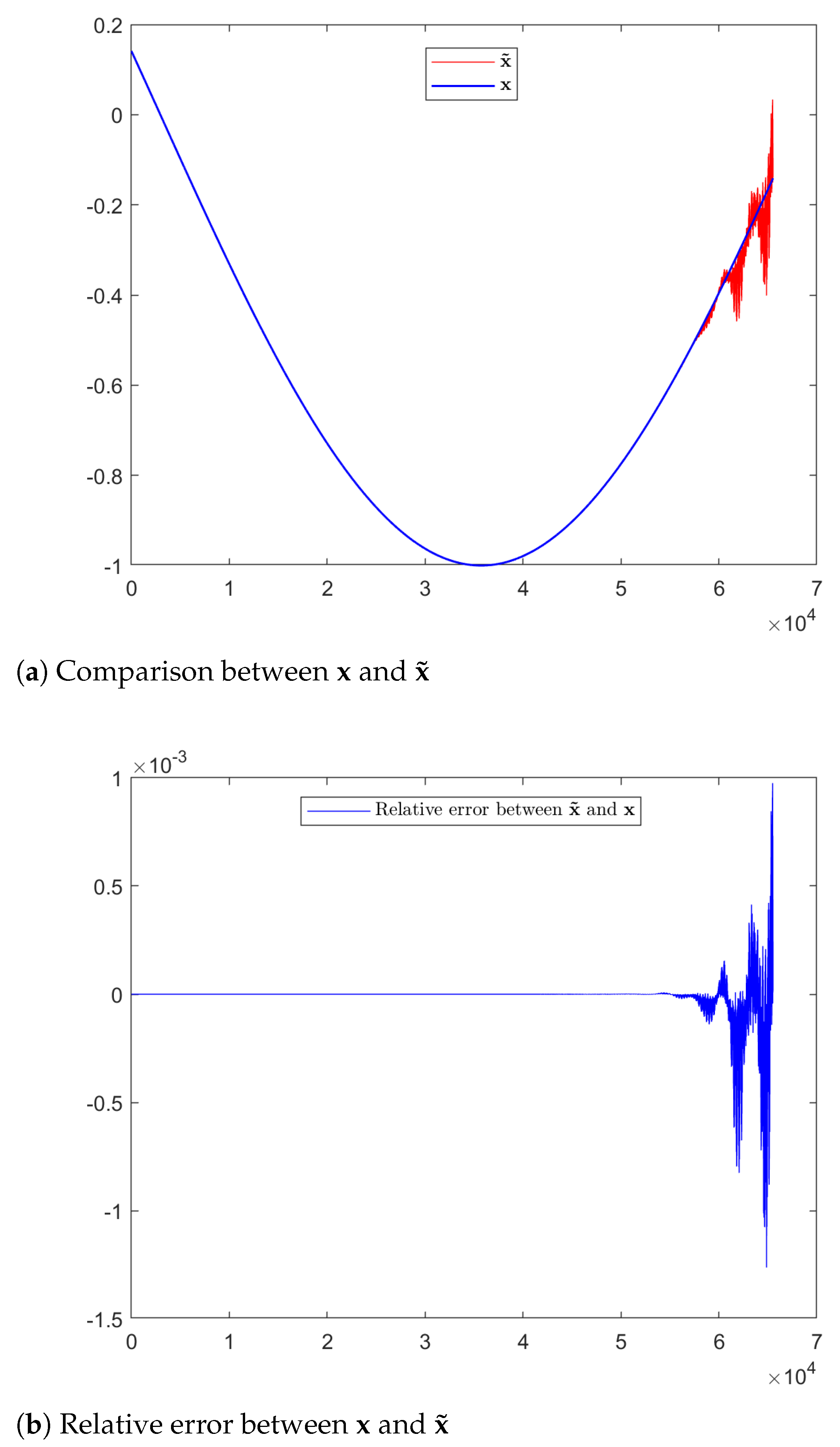
3.1. Parallel Solution of (Block) Triangular Toeplitz Systems

Since a diagonalization of $\omega$-circulant matrices through the Fourier matrix is available, it can be used to solve a linear system of the form ${\mathbf{C}}_{\omega }{\mathbf{x}}_{\omega }=\mathbf{r}$, with ${\mathbf{C}}_{\omega }$ as in Definition 2, ${\mathbf{x}}_{\omega },\mathbf{r}$$\in {\mathbb{R}}^n$ and $\omega \ne 0$, in an efficient way. More precisely, supposing that ${\mathbf{C}}_{\omega }$ is invertible and deriving from Proposition 2 the spectral decomposition

$${\mathbf{C}}_{\omega }^{-1}=D_{\omega }^{-1}{F}_n^{*}{L}_{n,\omega }^{-1}{F}_n{D}_{\omega },$$

${\mathbf{x}}_{\omega }$ can be calculated as the matrix-vector product ${\mathbf{C}}_{\omega }^{-1}\mathbf{r}$ via the following algorithm

• Compute $\mathbf{y}=F_n{D}_{\omega }\mathbf{r}$ via the FFT, with sequential cost $\mathcal{O}(nlog(n\left)\right)$;
• Compute $\mathbf{z}=L_{n,\omega }^{-1}\mathbf{y}$, with sequential cost $\mathcal{O}\left(n\right)$;
• Compute ${\mathbf{x}}_{\omega }=D_{\omega }^{-1}{F}_n^{*}\mathbf{z}$ via the FFT, with sequential cost $\mathcal{O}(nlog(n\left)\right)$.

This algorithm has a total sequential cost of $\mathcal{O}\left(n\log \right(n\left)\right)$, but, since all the steps can be fully parallelized, it can be lowered to $\mathcal{O}\left(\log \right(n\left)\right)$ in a parallel model of computation.

Now, the key idea to compute the solution of a (lower) triangular Toeplitz linear system $A\mathbf{x}=\mathbf{r}$, with $\mathbf{x},\mathbf{r}\in {\mathbb{R}}^n$ and

$$A=\left[\begin{array}{c}{a}_0\\ a_1& a_0\\ ⋮& \ddots & \ddots \\ a_{n-1}& \cdots & a_1& a_0\end{array}\right],a_0,a_1,\dots ,a_{n-1}\in \mathbb{C},$$

consists in completing A to the following $\omega$-circulant

$${\mathbf{C}}_{\omega }=\left[\begin{array}{cccc}{a}_0& \omega a_{n-1}& \cdots & \omega a_1\\ a_1& a_0& \ddots & ⋮\\ ⋮& \ddots & \ddots & \omega a_{n-1}\\ a_{n-1}& \cdots & a_1& a_0\end{array}\right]=A+\omega \left[\begin{array}{cccc}0& a_{n-1}& \cdots & a_1\\ & 0& \ddots & ⋮\\ & & \ddots & a_{n-1}\\ & & & 0\end{array}\right]$$

and observing that

$$\underset{\omega \to 0}{lim}{\mathbf{C}}_{\omega }^{-1}=A^{-1},\underset{\omega \to 0}{lim}{\mathbf{x}}_{\omega }^{-1}=\mathbf{x},\mathrm{where}{\mathbf{x}}_{\omega }={\mathbf{C}}_{\omega }^{-1}\mathbf{r}.$$

Hence, applying the algorithm described above, the solution of interest $\mathbf{x}$ can be approximated by computing ${\mathbf{x}}_{\omega }$, in theory up to an arbitrarily small error for $\omega \to 0$. Nevertheless, in practice an arbitrarily small error may not be attainable, since the condition number of the transform $F_n{D}_{\omega }$ corresponds to the condition number of $D_{\omega }$, which tends to $max\left\{\right|\omega |,|\omega {|}^{-1}\}$ as $n\to \infty$ and thus tends to infinity as $\omega \to 0$, causing stability issues. See the next subsection for a discussion in the setting of preconditioning.

The cost of this computation amounts to $\mathcal{O}\left(n\log \right(n\left)\right)$ in a sequential implementation and to $\mathcal{O}\left(\log \right(n\left)\right)$ in a parallel implementation. We refer the reader to Ref. [8] for details and two strategies that allow for the retrieval of the exact solution.

We stress that, although for the sake of clarity the above discussion takes into account the lower triangular case only, the technique can be easily extended to block triangular and upper triangular Toeplitz matrices.

3.2. Preconditioning for (Block) Triangular Toeplitz Systems

The algorithm described in the previous subsection can be applied in a very straightforward way to the preconditioning of linear systems with (block) triangular Toeplitz structure, allowing for an extremely efficient computation of the solution. On the other hand, special attention must be paid to the issue of stability, which strongly relies on the parameter $\omega$. We consider an example to present the approach, but we emphasize that the same basic ideas pertain to a variety of situations.

The example we use is taken from Ref. [21]. Here, Liu and Wu seek the numerical solution of the linear wave equation model

$$\left\{\begin{array}{cc}{y}_{tt}-\Delta y=f,\hfill & \mathrm{in}\Omega \times (0,T),\hfill \\ y=0,\hfill & \mathrm{on}\partial \Omega \times (0,T),\hfill \\ y(·,0)={\psi }_0,y_t(·,0)={\psi }_1\hfill & \mathrm{in}\Omega ,\hfill \end{array}\right.$$

(4)

where $\Omega \subset {\mathbb{R}}^d$ with $d>1$ is a bounded and open domain with Lipschitz boundary, ${\psi }_0$, ${\psi }_1$ are the initial conditions and f is a given source term. The equations are discretized all-at-once in time by means of implicit finite-difference schemes (see Ref. [21] for details). In the two-dimensional case with $\Omega$ a rectangle, the attained matrix shows the following block lower triangular Toeplitz structure

$$\mathcal{K}=\frac{1}{{\tau }^2}\left[\begin{array}{c}L\\ -2I_m& L\\ L& -2I_m& L\\ & \ddots & \ddots & \ddots \\ & & L& -2I_m& L\end{array}\right],L=I_m-\frac{{\tau }^2}{2}{\Delta }_h,$$

in which

• m is the number of grid nodes in the spatial mesh and $h=\frac{1}{m+1}$ is the spatial step size;
• $\tau$ is the time mesh step size, obtained as $\frac{T}{n}$, where n is the number of time steps;
• $I_m$ is the identity matrix of size m;
• ${\Delta }_h$ is the matrix obtained by discretizing the Laplacian operator $\Delta$ in (4) with the central finite difference method.

The associated linear system encompasses all the time steps at once and its solution corresponds to the solution to (4) at each time step simultaneously. In other words, if $y_j\in {\mathbb{R}}^m$ denotes the solution to (4) at the j-th time step, the system has the form

$$\mathcal{K}\mathbf{y}=\mathbf{b},\mathbf{y}=\left[\begin{array}{c}{y}_1\\ ⋮\\ y_n\end{array}\right],\mathbf{b}=\left[\begin{array}{c}{b}_1\\ ⋮\\ b_n\end{array}\right],b_j\in {\mathbb{R}}^m,j=1,\dots ,n$$

and therefore the vectors $y_j$, $j=1,\dots ,n$ are computed in parallel as the solution to the all-at-once linear system with the coefficient matrix $\mathcal{K}$.

To solve this linear system, the authors adopt a preconditioned GMRES method and construct a class of block $\omega$-circulant preconditioners as follows. Defining $B_1$ and $B_2$ as

$$B_1={\left[\begin{array}{c}1\\ 0& 1\\ 1& 0& 1\\ & \ddots & \ddots & \ddots \\ & & 1& 0& 1\end{array}\right]}_{n\times n},B_2={\left[\begin{array}{c}0\\ 1& 0\\ & 1& 0\\ & & \ddots & \ddots \\ & & & 1& 0\end{array}\right]}_{n\times n},$$

as described in Ref. [22], $\mathcal{K}$ can be expressed in the form

$$\mathcal{K}=\frac{1}{{\tau }^2}(B_1\otimes L-B_2\otimes 2I_m).$$

Then, given the matrix ${\Pi }_{n,\omega }$ as in Section 2 and

$${\Psi }_{n,\omega }=\left[\begin{array}{ccccc}1& & & \omega & 0\\ 0& 1& & & \omega \\ 1& 0& 1\\ & \ddots & \ddots & \ddots \\ & & 1& 0& 1\end{array}\right],$$

the generalized preconditioner is defined for $\omega \in (0,1]$ as

$${\mathcal{P}}_{\omega }=\frac{1}{{\tau }^2}\left({\Psi }_{n,\omega }\otimes L-{\Pi }_{n,\omega }\otimes 2I_m\right).$$

By exploiting the simultaneous diagonalization of the $\omega$-circulant matrices ${\Pi }_{n,\omega }$ and ${\Gamma }_{n,\omega }$ and the properties of the Kronecker product, ${\mathcal{P}}_{\omega }$ can be written as

$${\mathcal{P}}_{\omega }=\frac{1}{{\tau }^2}({\Gamma }_{\omega }^{-1}{F}_n^{*}\otimes I_m)(D_1\otimes L-2D_2\otimes I_m)(F_n{\Gamma }_{\omega }\otimes I_m),$$

where $F_n$ is the Fourier matrix, ${\Gamma }_{\omega }=\mathrm{diag}\left(1,{\omega }^{\frac{1}{n}},\dots ,{\omega }^{\frac{n-1}{n}}\right)$, $D_1=\mathrm{diag}\left(\sqrt{n}{F}_n{\Gamma }_{\omega }{\Psi }_{n,\omega }^{\left(1\right)}\right)$ and $D_2=\mathrm{diag}\left(\sqrt{n}{F}_n{\Gamma }_{\omega }{\Pi }_{n,\omega }^{\left(1\right)}\right)$, with ${\Psi }_{n,\omega }^{\left(1\right)}$, ${\Pi }_{n,\omega }^{\left(1\right)}$ being the first column of ${\Psi }_{n,\omega }$ and ${\Pi }_{n,\omega }$.

Therefore, given a vector $\mathbf{r}$, the proposed algorithm for computing $\mathbf{z}={\mathcal{P}}_{\omega }^{-1}\mathbf{r}$ is the following

• Compute ${\mathbf{s}}_1=(F_n{\Gamma }_{\omega }\otimes I_m)\mathbf{r}$ via the FFT;
• Compute ${\mathbf{s}}_2^{\left(k\right)}={\tau }^2{\left(D_1(k,k)L-2D_2(k,k)I_m\right)}^{-1}{\mathbf{s}}_1^{\left(k\right)}$, $k=1,\dots ,n$, where ${\mathbf{s}}_1^{\left(k\right)}$, ${\mathbf{s}}_2^{\left(k\right)}$ denote the k-th block of dimension m of ${\mathbf{s}}_1$, ${\mathbf{s}}_2$;
• Compute $\mathbf{z}=({\Gamma }_{\omega }^{-1}{F}_n^{*}\otimes I_m){\mathbf{s}}_2$ via the FFT;

Which in its essence is identical to the one proposed by Bini, although we must observe that Ref. [8] is not referenced in the work by Fan and Liu [21].

We conclude this section by discussing the matter of stability when dealing with $\omega$-circulants. While theoretically the aforementioned algorithm may be applied whenever $\omega \ne 0$, in practical implementation exceedingly small values of the parameter will cause stability issues, which should be considered, when stating the global precision of a solution method. In fact, as we mentioned in the previous section, the condition number of the transform $F_n{\Gamma }_{\omega }$ is equal to that of ${\Gamma }_{\omega }$, which tends to $max\left\{\right|\omega |,|\omega {|}^{-1}\}$ as $n\to \infty$ and therefore tends to infinity as $\omega \to 0$.

We tested the stability of the procedure described above by fixing a vector $\mathbf{x}$, computing $\mathbf{b}={\mathcal{P}}_{\omega }\mathbf{x}$ and retrieving the starting vector as ${\mathcal{P}}_{\omega }^{-1}\mathbf{b}$ with the spectral decomposition of ${\mathcal{P}}_{\omega }$, using the algorithm described above and in Ref. [21]. We denote the retrieved vector with $\tilde{\mathbf{x}}$.

As a first example, we set $m=2^8$, $n=2^8$, $\mathbf{x}={\left[\begin{array}{c}\sin \left(\frac{j\pi }{nm}+3\right)\end{array}\right]}_{j=1,\dots ,nm}$ and show the relative errors between $\mathbf{x}$ and $\tilde{\mathbf{x}}$ as the parameter $\omega$ decreases in Table 1. Clearly, as $\omega$ gets closer to zero, the error grows and $\tilde{\mathbf{x}}$ ceases to be an accurate approximation of $\mathbf{x}$, especially in the right part in accordance with the accumulation errors in the solution of a lower triangular system. In particular the error for very small values of $\omega$ becomes even worse than that obtained when using a direct inherently sequential algorithm working for triangular systems ($\omega =0$). Figure 1 shows the plots of the two vectors for $\omega ={10}^{-16}$.

Table 1. The relative error between $\mathbf{x}={\left[\begin{array}{c}\sin \left(\frac{j\pi }{nm}+3\right)\end{array}\right]}_{j=1,\dots ,nm}$ and $\tilde{\mathbf{x}}$ as $\omega$ decreases.

$\mathit{\omega }$	$\frac{\parallel \mathit{x}-\tilde{\mathit{x}}\parallel }{\parallel \mathit{x}\parallel }$
${10}^{-2}$	$1.81\times {10}^{-14}$
${10}^{-4}$	$4.93\times {10}^{-13}$
${10}^{-6}$	$1.52\times {10}^{-11}$
${10}^{-8}$	$1.28\times {10}^{-9}$
${10}^{-10}$	$1.15\times {10}^{-7}$
${10}^{-12}$	$7.47\times {10}^{-6}$
${10}^{-14}$	$4.76\times {10}^{-4}$
${10}^{-16}$	$2.20\times {10}^{-2}$
${10}^{-18}$	$1.23\times 10$

Figure 1. $\mathbf{x}={\left[\begin{array}{c}\sin \left(\frac{j\pi }{nm}+3\right)\end{array}\right]}_{j=1,\dots ,nm}$ and $\tilde{\mathbf{x}}$ for $\omega ={10}^{-16}$.

Our second example, where $\mathbf{x}$ is this time chosen at random, grants similar results, collected in Table 2. We observe that this matter is not addressed in Ref. [21].

Table 2. The relative error between $\mathbf{x}$ randomly chosen and $\tilde{\mathbf{x}}$ as $\omega$ decreases.

$\mathit{\omega }$	$\frac{\parallel \mathit{x}-\tilde{\mathit{x}}\parallel }{\parallel \mathit{x}\parallel }$
${10}^{-2}$	$4.06\times {10}^{-14}$
${10}^{-4}$	$1.84\times {10}^{-12}$
${10}^{-6}$	$6.04\times {10}^{-11}$
${10}^{-8}$	$5.80\times {10}^{-9}$
${10}^{-10}$	$8.41\times {10}^{-7}$
${10}^{-12}$	$4.96\times {10}^{-5}$
${10}^{-14}$	$6.31\times {10}^{-3}$
${10}^{-16}$	$2.18\times {10}^{-1}$
${10}^{-18}$	$6.13\times 10$

Because of these instability issues, the possibility of using preconditioned MINRES recently emerged, where the preconditioner is taken from the $\tau$ algebra whose eigenvector matrix can be chosen as a real symmetric orthogonal and very stable transform (see Ref. [22] and the references therein). This type of methods, called all-at-once, have attracted a remarkable attention in the last 10 years for the potential use in parallel in time methods for evolution of PDEs; see Refs. [23,24,25,26] and their references. Further works on the matter can be found in Refs. [27,28], also for fractional differential equations.

We now consider the second application of $\omega$-circulants in the context of subdivision schemes for generating curves and surfaces.

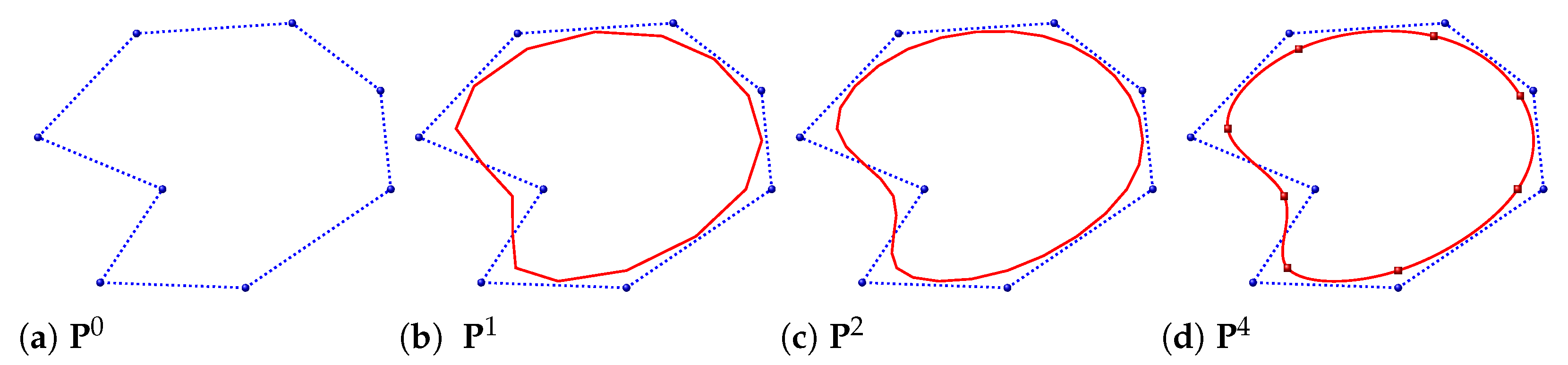
4. Basic Ideas on Scalar Subdivision Schemes

A subdivision scheme is an iterative method that generates curves and surfaces based on successive refinements of a polygon or a mesh. The rules that determine said refinements can be formulated by linear, non-linear, or geometrical operators [29,30,31,32,33]. The case of linear rules is related to refinable functions in Wavelets Theory [34]. In this setting, the vertices of the polygon or mesh are the coefficients in a particular basis of the so-called subdivision curve or subdivision surface. In what follows we focus on the case of the subdivision curve.

Linear uniform subdivision schemes are based on the notion of refinable function, i.e., a function $\phi \left(t\right)$ satisfying a relation of the form

$$\phi \left(t\right)=\sum _{j\in \mathbb{Z}}{a}_j\phi (2t-j),t\in \mathbb{R},a_j\in \mathbb{R}$$

(5)

and such that, given an initial set of control points ${\mathbf{P}}^0=\{P_j^0\in {\mathbb{R}}^m,j=0,\dots ,n-1\}$ and the periodisation $P_j^0=P_{j+n}^0$, $\forall j\in \mathbb{Z}$, the closed curve

$$c\left(t\right)=\sum _{j\in \mathbb{Z}}{P}_j^0\phi (t-j),t\in \mathbb{R}$$

(6)

can also be written as

$$c\left(t\right)=\sum _{j\in \mathbb{Z}}{P}_j^k\phi \left(2^{k}t-j\right),t\in \mathbb{R}$$

with

$$P_i^{k+1}=\sum _{j\in \mathbb{Z}}{a}_{i-2j}{P}_j^k,k\in \mathbb{N},i=0,\dots ,2^{k+1}n-1,$$

(7)

where for the set ${\mathbf{P}}^k$ of new points the periodisation modulo $2^{k}n$ holds, i.e., $P_j^k=P_{j+2^{k}n}^k$, $j\in \mathbb{Z}$.

The relation in (7) is known as the subdivision rule and defines a subdivision scheme, while the coefficients $\mathbf{a}=\{a_j,j\in \mathbb{Z}\}$ in (5) form the so-called subdivision mask. Then, a subdivision scheme is an iterative method where a curve is generated by consecutive refinements of an initial polygon (see Figure 2). Regarding the convergence of this scheme, it has been proven that the sequence of polygons with vertices in ${\mathbf{P}}^k$ converges uniformly to a smooth curve $c\left(t\right)$, although in practice a few iterations are sufficient to produce a polygon that appears smooth to the human eye.

Figure 2. Iterations of a non-interpolatory subdivision scheme. (a) Control points ${\mathbf{P}}^0$ (blue balls). (b) First refinement of the polygon with vertices ${\mathbf{P}}^1$. (c) Second refinement with vertices ${\mathbf{P}}^2$. (d) Fourth refinement and interpolated points ${\mathbf{V}}^0$ in the limit (red squares).

The sampling of the curve at integer parameters is derived from (5) and reads as

$$c\left(s\right)=\sum _{j\in \mathbb{Z}}{P}_j^0\phi \left(s-j\right),t\in \mathbb{Z},s\in \mathbb{Z}.$$

(8)

The set of values ${\beta }^0=\left\{{\beta }_j^0=\phi \left(j\right),j\in \mathbb{Z}\right\}$ is called first limit stencil and it can be obtained from a linear system of equations stemming from (5) (see Ref. [35]) or by performing the spectral analysis of the local subdivision matrix (see Refs. [33,36,37]). In a similar way, the second limit stencil and higher order stencils ${\beta }^{k-1}=\left\{{\beta }_j^{k-1}={\phi }^{(k-1)}\left(j\right),j\in \mathbb{Z}\right\}$, $k\in \mathbb{N}$, $k\ge 1$ can be determined. Hence, by (6) the k-th derivative of the curve at dyadic parameters $t=\mathbb{Z}/2^m$ is

$$c^{\left(k\right)}\left(\frac{s}{2^m}\right)=\sum _{j\in \mathbb{Z}}{\beta }_{s-j}^k{P}_j^m.$$

(9)

The mask and the stencils have compact support and therefore in (5) they define a function that has compact support. Even though we use indexes ranging over $\mathbb{Z}$, we are dealing with finite masks and stencils and correspondingly we have only a finite number of non-zero elements.

Given the control points ${\mathbf{P}}^0$, let us denote with ${\mathbf{V}}^0=\{V_j^0\in {\mathbb{R}}^m,j=0,\dots ,n-1\}$ the points obtained by evaluating the subdivision curve with (8), i.e., $V_j^0=c\left(j\right)$, $j=0,\dots ,n-1$ (see Figure 2d). This problem is modeled by the linear operator $M_n$ such that

$$M_n{\mathbf{P}}^0=\left[\begin{array}{cccccc}{\beta }_0& {\beta }_{-1}& {\beta }_{-2}& \dots & {\beta }_2& {\beta }_1\\ {\beta }_1& {\beta }_0& {\beta }_{-1}& \dots & {\beta }_3& {\beta }_2\\ \ddots & \ddots & \ddots & \ddots & \ddots & \ddots \\ {\beta }_{-1}& {\beta }_{-2}& {\beta }_{-3}& \dots & {\beta }_1& {\beta }_0\end{array}\right]\left[\begin{array}{c}{P}_0^0\\ P_1^0\\ ⋮\\ P_{n-1}^0\end{array}\right]=\left[\begin{array}{c}{V}_0^0\\ V_1^0\\ ⋮\\ V_{n-1}^0\end{array}\right]=\left[\begin{array}{c}c\left(0\right)\\ c\left(1\right)\\ ⋮\\ c(n-1)\end{array}\right].$$

(10)

$M_n$ is referred to as the matrix that represents the point interpolation operator for linear subdivision schemes. Note that the structure of $M_n$ is circulant, according to Definition 1, and the first row is the vector

$${\beta }_n:=\left[{\beta }_0,{\beta }_{-1},\dots ,{\beta }_{-p},0,\dots ,0,{\beta }_q,\dots ,{\beta }_1\right]\in {\mathbb{R}}^m.$$

Depending on the symmetry of the stencils, some particular cases may be analysed.

Definition 4.

A subdivision scheme is called

• Odd-symmetric if $a_{-j}=a_j$;
• Even-symmetric if $a_{1-j}=a_j$ for $j\in \mathbb{N}$.

This definition contains particular cases of the primal [38] and dual [39] form of subdivision schemes, respectively, and the corresponding limit stencils show the same type of symmetries [33]. As a consequence, the odd-order limit stencil inherits the odd or even symmetry:

$${\beta }_j^{2d}=\left\{\begin{array}{cc}{\beta }_{-j}^{2d},\hfill & \mathrm{for}\mathrm{odd}-\mathrm{symmetric}\mathrm{schemes},\hfill \\ {\beta }_{1-j}^{2d},\hfill & \mathrm{for}\mathrm{even}-\mathrm{symmetric}\mathrm{schemes},\hfill \end{array}\right.d\in \mathbb{N}.$$

(11)

Then, for the even-order limit stencil we get

$${\beta }_j^{2d+1}=\left\{\begin{array}{cc}-{\beta }_{-j}^{2d+1}\hfill & \mathrm{for}\mathrm{odd}-\mathrm{symmetric}\mathrm{schemes},\hfill \\ -{\beta }_{1-j}^{2d+1}\hfill & \mathrm{for}\mathrm{even}-\mathrm{symmetric}\mathrm{schemes},\hfill \end{array}\right.d\in \mathbb{N}.$$

(12)

For $d\ge 1$ it holds ${\displaystyle \sum _{j\in \mathbb{Z}}{\beta }_j^d=0}$ and ${\displaystyle \sum _{j\in \mathbb{Z}}{\beta }_j^0=1}$.

Now, let us consider the interpolation of n points ${\mathbf{V}}^0$ with a subdivision curve. It is natural to think of those points as a sampling of the curve at integer parameters $V_s^0=c\left(s\right)$, $s=0,\dots ,n-1$, as in (8). By doing so, we get the inverse problem with respect to (10) (see Ref. [40]).

In this setting, an interpolation problem is said to be singular if the operator $M_n$ is singular and therefore ill-posed for the selected stencil. In Section 5, we show that in some cases the singularity depends on the value of n.

To solve a non-singular interpolation problem where $M_n$ has a circulant structure, one can take advantage of the diagonalization through the Fourier matrix recalled in Section 2. However, in the singular case more strategy is needed. In the literature, in the context of curve and surface schemes those cases are treated by a fitting model [41] or by a fairness functional [42] while introducing more points as degrees of freedom. Another possible approach consists in the regularization in a Tikhonov sense [40,43]. Moreover, it is possible to consider a non-singular perturbation of the matrix $M_n$. This is the strategy that we explore in Section 5.2, using a computationally convenient $\omega$-circulant matrix.

The Block-Circulant Case for Hermite Interpolation

Considering the case of interpolating points and associated derivatives up to the $(d-1)$-th order, with tangent interpolation as the first instance, Equation (9) provides some insight. Let ${\mathbf{U}}^{\left(d\right)}={[V_0^0,V_0^1,\dots ,V_0^{d-1},V_1^0,V_1^1,\dots ,V_1^{d-1},\dots ,V_{n-1}^0,V_{n-1}^1,\dots ,V_{n-1}^{d-1}]}^{\top }$ be the data that we wish to interpolate and suppose that there exists a sequence $\left\{t_j,j=0,\dots ,n-1\right\}$ such that the subdivision curve $c\left(t\right)$ interpolates the data ${\mathbf{U}}^{\left(d\right)}$, i.e.,

$$c^{\left(k\right)}\left(t_j\right)=V_j^k,\mathrm{for}k=0,\dots ,d-1,j=0,\dots ,n.$$

(13)

If the curve $c\left(t\right)$ is defined by n control points as in (10), we may get a solution to the point interpolation problem (10) that contradicts the values of higher order derivatives. Thus, in order to interpolate all the information in ${\mathbf{U}}^{\left(d\right)}$ with an equal amount of variables and equations, we need to use $nd$ control points ${\mathbf{P}}^0=\{P_j^0\in {\mathbb{R}}^m,j=0,\dots ,nd-1\}$ with the periodisation $P_j^0=P_{j+nd}^0$, $j\in \mathbb{Z}$. A natural choice is to set the parameters in (13) as $t_j=dj$, $j=0,\dots ,n-1$. Then, from (9) we get the $nd$ equations

$$c^{\left(k\right)}\left(dj\right)=V_j^k=\sum _{j\in \mathbb{Z}}{P}_s^0{\beta }_{dj-s}^k,j=0,\dots ,n-1,k=0,\dots ,d-1,$$

which can be represented in matrix form as

$${\mathbf{M}}_n{\mathbf{P}}^0=\left[\begin{array}{cccccc}{\mathit{B}}_0& {\mathit{B}}_{-1}& {\mathit{B}}_{-2}& \dots & {\mathit{B}}_2& {\mathit{B}}_1\\ {\mathit{B}}_1& {\mathit{B}}_0& {\mathit{B}}_{-1}& \dots & {\mathit{B}}_3& {\mathit{B}}_2\\ \ddots & \ddots & \ddots & \ddots & \ddots & \ddots \\ {\mathit{B}}_{-1}& {\mathit{B}}_{-2}& {\mathit{B}}_{-3}& \dots & {\mathit{B}}_1& {\mathit{B}}_0\end{array}\right]\left[\begin{array}{c}{P}_0^0\\ P_1^0\\ ⋮\\ P_{nd-1}^0\end{array}\right]={\mathbf{U}}^{\left(d\right)},$$

(14)

where the $d\times d$ blocks of the matrix ${\mathbf{M}}_n\in {\mathbb{R}}^{nd\times nd}$ satisfy ${\mathbf{B}}_j={\mathbf{B}}_{j-n}$ for $j=1,\dots ,n$ and

$${\mathit{B}}_j=\left[\begin{array}{ccccc}{\beta }_{dj}^0& {\beta }_{dj-1}^0& {\beta }_{dj-2}^0& \dots & {\beta }_{d(j-1)+1}^0\\ {\beta }_{dj}^1& {\beta }_{dj-1}^1& {\beta }_{dj-2}^1& \dots & {\beta }_{d(j-1)+1}^1\\ \ddots & \ddots & \ddots & \ddots & \ddots \\ {\beta }_{dj}^{d-1}& {\beta }_{dj-1}^{d-1}& {\beta }_{dj-2}^{d-1}& \dots & {\beta }_{d(j-1)+1}^{d-1}\end{array}\right].$$

(15)

The structure of the matrix in (14) is the block adaptation of the scalar version (10), i.e., it is a block circulant matrix, as described in Definition 3. Indeed, when $d=1$, ${\mathbf{M}}_n\equiv M_n$ and ${\mathbf{U}}^{\left(1\right)}\equiv {\mathbf{V}}^0$. Therefore, the Hermite problem represents the block extension of the point interpolation problem in the matrix sense and we can exploit the corresponding linear algebra tools to solve both inverse problems.

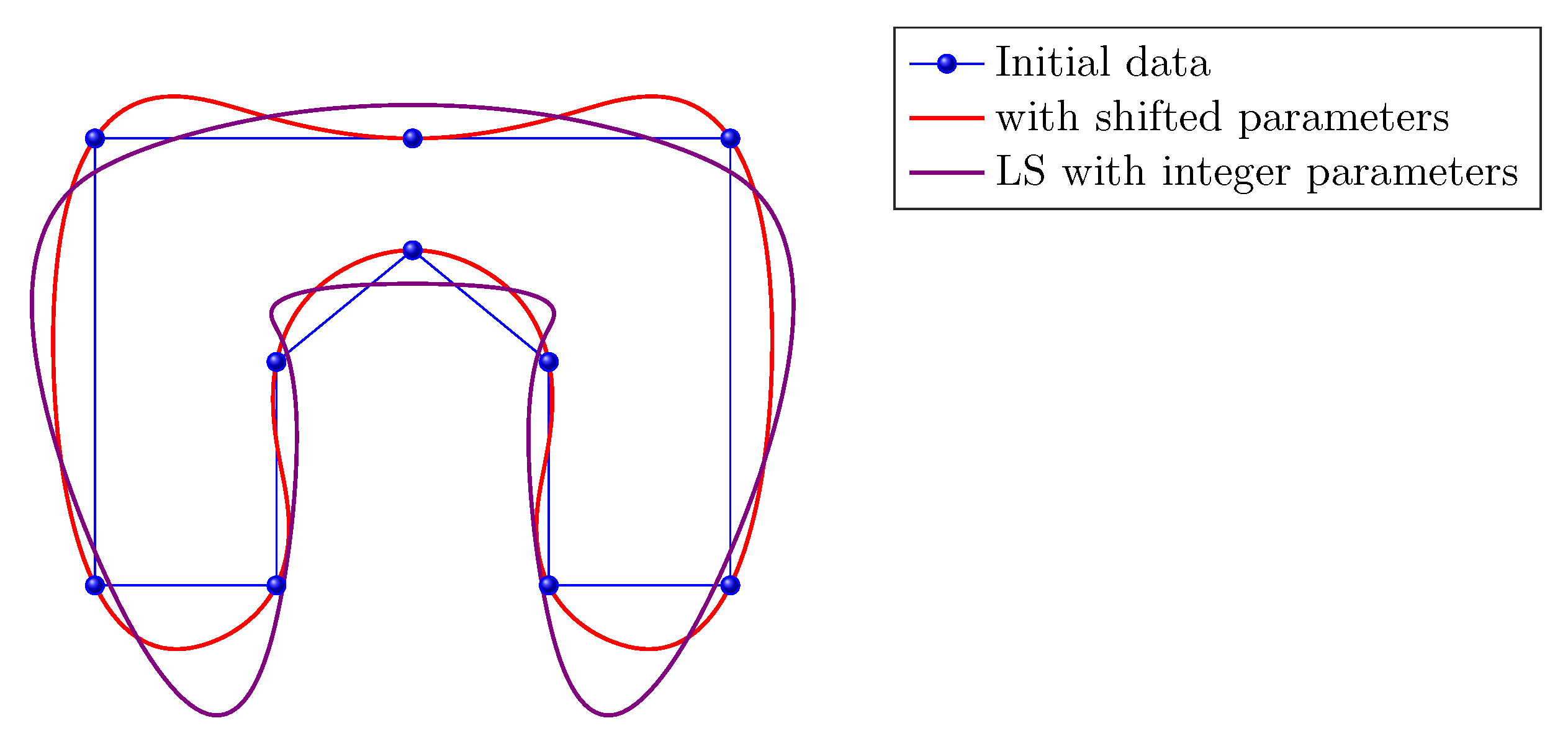
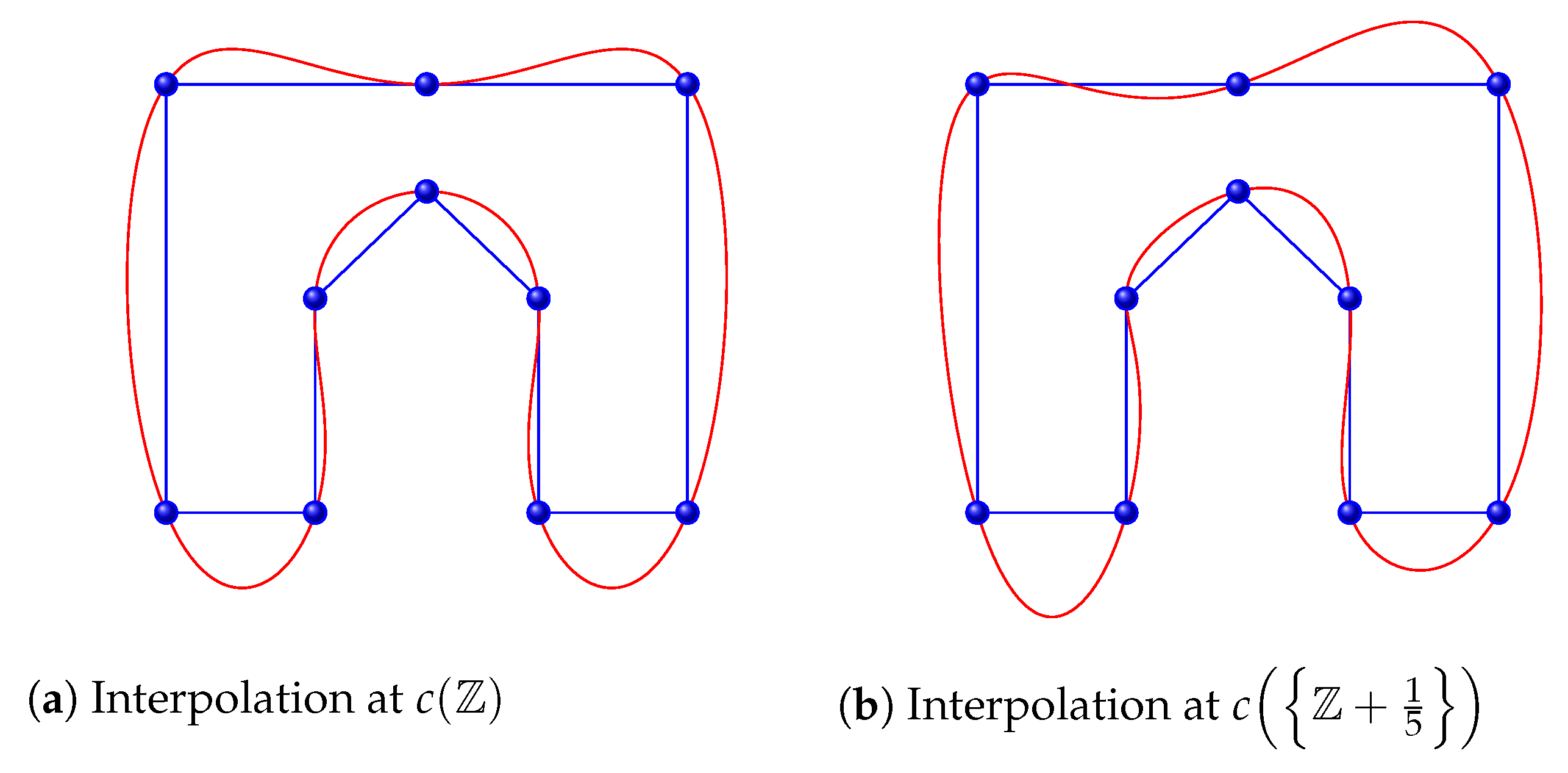
5. Interpolation Model with Scalar Subdivision Schemes

Given the problem $M_n{\mathbf{P}}^0={\mathbf{V}}^0$ in (10), let us apply the tools available for circulant matrices to solve it. Indeed, by Remark 1 we deduce that the spectrum of $M_n$ is

$$\Lambda \left(M_n\right)=\left\{b\left(\frac{2\pi j}{n}\right),j=0,\dots ,n-1\right\}$$

(16)

and for the stencils with compact support in $[-p,q]$ the symbol can be written as

$$b\left(\theta \right):=\sum _{k=-p}^q{\beta }_{k}exp\left(\mathrm{i}k\theta \right),$$

independent of n. Thus, the singularity of $M_n$ depends on the existence of roots for $b\left(\theta \right)$ in the grid $\frac{2\pi \mathbb{N}}{n}\cap [0,2\pi ]$.

For odd-symmetric schemes, ${\mathit{\beta }}_n:=\left[{\beta }_0,{\beta }_{-1},\dots ,{\beta }_{-p},0,\dots ,0,{\beta }_p,\dots ,{\beta }_1\right]\in {\mathbb{R}}^n$ and thus

$$b\left(\theta \right)=\sum _{k=-p}^p{\beta }_{k}exp\left(\mathrm{i}k\theta \right)={\beta }_0+2\sum _{k=1}^p{\beta }_{k}cos\left(k\theta \right).$$

(17)

Conversely, for even-symmetric schemes ${\mathit{\beta }}_n:=$$\left[{\beta }_0,{\beta }_{-1},\dots ,{\beta }_{-p+1},0,\dots ,0,{\beta }_p,\dots ,{\beta }_1\right]\in {\mathbb{R}}^n$, hence

$$\begin{array}{cc}\hfill b\left(\theta \right)& =\sum _{k=-p+1}^p{\beta }_{k}exp\left(\mathrm{i}k\theta \right)=\sum _{k=1}^p{\beta }_k\left(exp\left(\mathrm{i}\right(-k+1\left)\theta \right)+exp\left(\mathrm{i}k\theta \right)\right)\hfill \\ \hfill & =exp\left(\frac{\mathrm{i}\theta }{2}\right)\sum _{k=1}^p{\beta }_k\left(exp\left(\mathrm{i}\left(-k+\frac{1}{2}\right)\theta \right)+exp\left(\mathrm{i}\left(k-\frac{1}{2}\right)\theta \right)\right)\hfill \\ \hfill & =2exp\left(\frac{\mathrm{i}\theta }{2}\right)\sum _{k=1}^p{\beta }_{k}cos\left((2k-1)\frac{\theta }{2}\right).\hfill \end{array}$$

(18)

Either way, the first limit stencil satisfies $b\left(0\right)=1$. Note that for odd-symmetric schemes it holds

$$b(2\pi -\theta )={\beta }_0+2\sum _{k=1}^p{\beta }_{k}cos\left(k(2\pi -\theta )\right)={\beta }_0+2\sum _{k=1}^p{\beta }_{k}cos\left(k\theta \right)=b\left(\theta \right),$$

while for the even-symmetric schemes

$$\begin{array}{cc}\hfill b(2\pi -\theta )& =2exp\left(\frac{\mathrm{i}(2\pi -\theta )}{2}\right)\sum _{k=0}^p{\beta }_{k}cos\left((2k-1)\frac{(2\pi -\theta )}{2}\right)\hfill \\ \hfill & =2exp\left(\frac{-\mathrm{i}\theta }{2}\right)\sum _{k=0}^p{\beta }_{k}cos\left((2k-1)\frac{\theta }{2}\right)\hfill \\ \hfill & =exp(-\mathrm{i}\theta )b\left(\theta \right).\hfill \end{array}$$

Therefore, the study of the symbol can be restricted to the interval $[0,\pi ]$ instead of $[0,2\pi ]$. In particular, for both (17) and (18), $b\left(\theta \right)=0$ implies $b(2\pi -\theta )=0$.

From (18), for even-symmetric schemes we find $b\left(\pi \right)=0$ independently of n and $\mathit{\beta }$. As $\pi$ belongs to the grid $\frac{2\pi \mathbb{N}}{n}\cap [0,2\pi ]$ for even values of n, then from (16) we obtain the following result.

Proposition 4.

For any even-symmetric subdivision scheme, if the amount of interpolated points n is even, then the interpolation matrix $M_n$ is singular.

On the other hand, in the context of odd-symmetric schemes the symbol may also vanish in the grid $\frac{2\pi \mathbb{N}}{n}\cap [0,2\pi ]$. As an example, consider the primal family of J-spline schemes [38] for the particular case that generates $C^3$ subdivision curves

$$\left\{\begin{array}{cc}{P}_{2j}^{k+1}\hfill & =\frac{1}{4}{P}_{j-1}^k+\frac{1}{2}{P}_j^k+\frac{1}{4}{P}_{j+1}^k,\hfill \\ P_{2j+1}^{k+1}\hfill & =\frac{1}{16}{P}_{j-1}^k+\frac{7}{16}{P}_j^k+\frac{7}{16}{P}_{j+1}^k+\frac{1}{16}{P}_{j+2}^k,k\in \mathbb{N},j\in \mathbb{Z},\hfill \end{array}\right.$$

(19)

with first limit stencil

$$\mathit{\beta }=\frac{1}{48}\left\{1,12,22,12,1\right\}.$$

The symbol

$$b\left(\theta \right)=\frac{11}{24}+\frac{1}{2}cos\left(\theta \right)+\frac{1}{24}cos\left(2\theta \right)=(cos\left(\theta \right)+1)\left(cos\left(\theta \right)+\frac{1}{5}\right)$$

has a root at $\theta =\pi$, which belongs to the grid $\frac{2\pi \mathbb{N}}{n}\cap [0,2\pi ]$ when n is an even number.

In the Hermite interpolation scenario, we can find a singular point and tangents interpolation operator even when the point interpolation operator is not singular. Let us consider for instance the cubic B-spline scheme, whose first and second limit stencil are $\{\frac{1}{6},\frac{4}{6},\frac{1}{6}\}$$\{-\frac{1}{2},0,\frac{1}{2}\}$, respectively. Then the corresponding matrices are

$$\left[\begin{array}{cccccc}\frac{4}{6}& \frac{1}{6}& 0& \dots & 0& \frac{1}{6}\\ \frac{1}{6}& \frac{4}{6}& \frac{1}{6}& \dots & 0& 0\\ ⋮& \ddots & \ddots & \ddots & \ddots & ⋮\\ \frac{1}{6}& 0& 0& \dots & \frac{4}{6}& \frac{1}{6}\end{array}\right],$$

which is not singular, and

$$\left[\begin{array}{ccccc}\begin{array}{cc}\frac{4}{6}& \phantom{-}\frac{1}{6}\\ 0& \phantom{-}\frac{1}{2}\end{array}& \begin{array}{cc}0& \phantom{-}0\\ 0& \phantom{-}0\end{array}& \dots & \begin{array}{cc}0& \phantom{-}0\\ 0& \phantom{-}0\end{array}& \begin{array}{cc}0& \phantom{-}\frac{1}{6}\\ 0& -\frac{1}{2}\end{array}\\ \begin{array}{cc}0& \phantom{-}\frac{1}{6}\\ 0& -\frac{1}{2}\end{array}& \begin{array}{cc}\frac{4}{6}& \phantom{-}\frac{1}{6}\\ 0& \phantom{-}\frac{1}{2}\end{array}& \ddots & \begin{array}{cc}0& \phantom{-}0\\ 0& \phantom{-}0\end{array}& \begin{array}{cc}0& \phantom{-}0\\ 0& \phantom{-}0\end{array}\\ ⋮& \ddots & \ddots & \ddots & ⋮\\ \begin{array}{cc}0& \phantom{-}0\\ 0& \phantom{-}0\end{array}& \begin{array}{cc}0& \phantom{-}0\\ 0& \phantom{-}0\end{array}& \dots & \begin{array}{cc}0& \phantom{-}\frac{1}{6}\\ 0& -\frac{1}{2}\end{array}& \begin{array}{cc}\frac{4}{6}& \phantom{-}\frac{1}{6}\\ 0& \phantom{-}\frac{1}{2}\end{array}\end{array}\right]$$

which is singular with kernel of dimension 1.

As a matter of fact, in the specific case of point and tangent interpolation with odd-symmetric schemes, the following proposition holds.

Proposition 5.

Using an odd-symmetric subdivision scheme and setting $d=2$, the attained matrix ${\mathbf{M}}_n$ is singular.

Proof. 

From (3) and (15), for odd-symmetric schemes we have that the $(1,1)$-block of ${\mathcal{L}}_n$ is:

$$\begin{array}{cc}\hfill {\left({\mathcal{L}}_n\right)}_{1,1}& =\sum _{j=0}^{\lceil \frac{p}{2}\rceil }\left[\begin{array}{cc}{\beta }_{-2j}^0& {\beta }_{-2j-1}^0\\ {\beta }_{-2j}^1& {\beta }_{-2j-1}^1\end{array}\right]+\sum _{j=1}^{\lceil \frac{p}{2}\rceil }\left[\begin{array}{cc}{\beta }_{2j}^0& {\beta }_{2j-1}^0\\ {\beta }_{2j}^1& {\beta }_{2j-1}^1\end{array}\right]\hfill \\ \hfill & =\left[\begin{array}{cc}{\beta }_0^0& {\beta }_1^0\\ {\beta }_0^1& -{\beta }_1^1\end{array}\right]+\sum _{j=1}^{\lceil \frac{p}{2}\rceil }\left[\begin{array}{cc}{\beta }_{2j}^0& {\beta }_{2j-1}^0\\ -{\beta }_{2j}^1& -{\beta }_{2j+1}^1\end{array}\right]+\sum _{j=1}^{\lceil \frac{p}{2}\rceil }\left[\begin{array}{cc}{\beta }_{2j}^0& {\beta }_{2j-1}^0\\ {\beta }_{2j}^1& {\beta }_{2j-1}^1\end{array}\right]\hfill \\ \hfill & =\left[\begin{array}{cc}{\displaystyle {\beta }_0^0+2\sum _{j=1}^{\lceil \frac{p}{2}\rceil }{\beta }_{2j}^0}& {\displaystyle 2\sum _{j=1}^{\lceil \frac{p}{2}\rceil }{\beta }_{2j-1}^0}\\ 0& 0\end{array}\right],\hfill \end{array}$$

(20)

where we used the fact that ${\beta }_0^1=0$ from (12). The block ${\left({\mathcal{L}}_n\right)}_{1,1}$ is singular, since it has a null row, and the matrices ${\mathcal{L}}_n$ and ${\mathbf{M}}_n$ are in turn singular because of (3). □

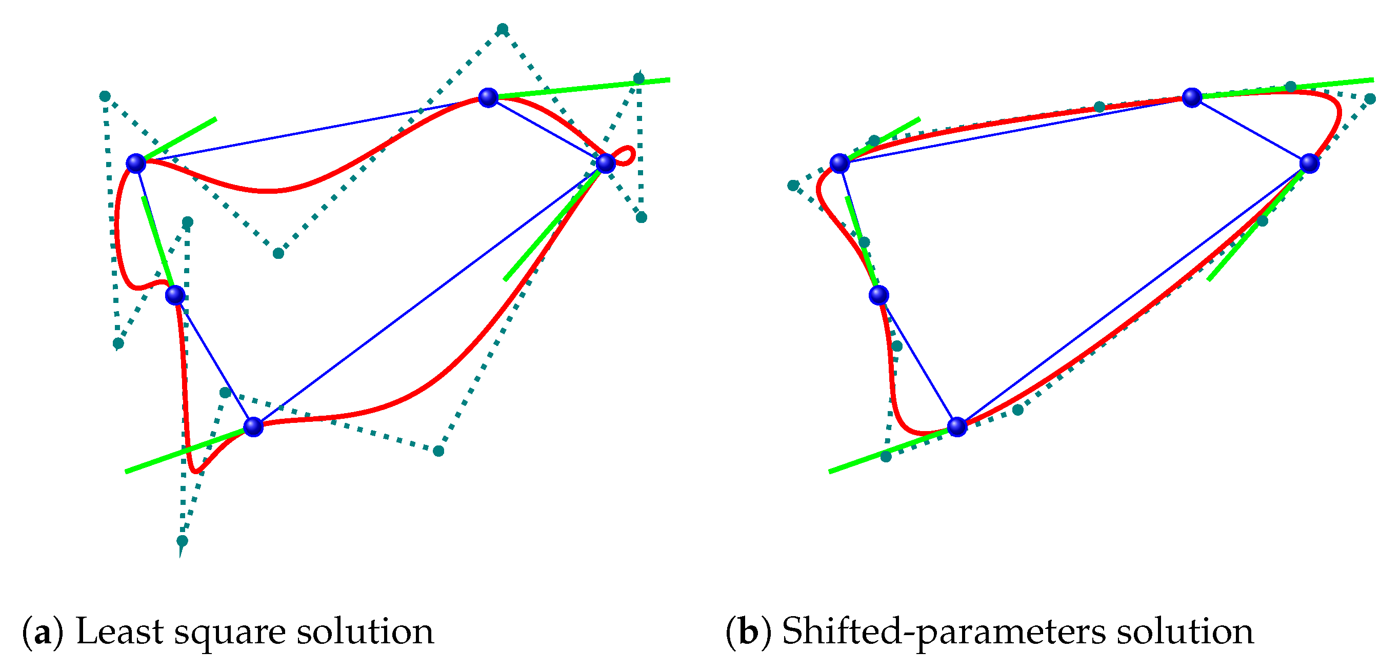
5.1. A Solution by Shifting Parameters

Propositions 4 and 5 state that, for even-symmetric and odd-symmetric masks, the matrices $M_n$ and ${\mathbf{M}}_n$ are singular independently of the mask. In this section, we propose a different model for interpolating that avoids this inconvenience. What follows is motivated by Plonka’s work [44] on Hermite interpolation with B-spline parametric curves.

Let us consider the dual subdivision schemes again. In Section 4, by interpolating at the parameters $t_j=j$, $j=0,\dots ,n-1$, we obtained the first limit stencil as

$$V_j^0=c\left(j\right)=\sum _{s\in \mathbb{Z}}\phi (j-s)P_s^0=\sum _{s=-p}^q\phi \left(s\right)P_{j-s}^0,\mathrm{with}\mathrm{supp}\phi =[-p,q].$$

Here we consider the variant

$$V_j^0=c(j+\sigma )=\sum _{s\in \mathbb{Z}}\phi (j-s+\sigma )P_s^0=\sum _{s=-p}^{q-1}\phi (s+\sigma )P_{j-s}^0$$

with $\sigma \in (0,1)$. More specifically, given a positive integer $\nu$, we investigate the method for $\sigma$ varying in $\frac{1}{\nu }\mathbb{Z}\cap (0,1)$. The evaluation of the basic function is done as in [35].

In the case of symmetric masks, as in (11) and (12), the following results hold.

Proposition 6.

For an odd-symmetric subdivision scheme with mask $\mathbf{a}=\{a_{-p},a_{-p+1},\dots ,a_p\}$ where $p\in \mathbb{N}$, the stencil obtained with the set $\phi \left(\frac{1}{2}+\mathbb{Z}\right)\cap [-p,p]$ is even-symmetric.

Analogously, for an even-symmetric subdivision scheme with mask $\mathbf{a}=\{a_{-p},a_{-p+1},\dots ,a_{p+1}\}$ where $p\in \mathbb{N}$, the stencil obtained with the set $\phi \left(\frac{1}{2}+\mathbb{Z}\right)\cap [-p,p+1]$ is odd-symmetric.

Our proposal consists in modifying the interpolation models (10) and (14) to $c^{\left(k\right)}\left(\frac{1}{2}+dj\right)=V_j^k$. For point interpolation, the symbol changes from (18) to (17) and this way we resolve the singularity in Proposition 4. Figure 3 portrays an example of even-symmetric subdivision scheme where after a $\frac{1}{2}$-shift the new matrix is nonsingular. However, when the new stencil leads to a trigonometric polynomial with roots in the grid $\frac{1}{n}\mathbb{Z}\cap [0,1]$ it is not possible to avoid the singularity of the corresponding matrix. In such situations, one may consider the general approach $V_j^0=c(j+\sigma )$, with $\sigma \in (0,1)$ or treat the singularity as discussed in the next subsection.

Figure 3. Point interpolation with a dual subdivision scheme [39] considering the shifted parameters.

The use of shifted parameters for interpolation can be employed as a degree of freedom for the geometry of the interpolation curve (see Figure 4). Nevertheless, the symmetry provided by the subdivision scheme might be lost.

Figure 4. Interpolation with quintic uniform B-spline at different parameter values.

Now let us consider the point and tangent interpolation with the interpolation at the parameters $\frac{1}{2}+\mathbb{Z}$ for odd-symmetric schemes. The first block (20) in the factorization of ${\mathbf{M}}_n$ becomes

$$\begin{array}{cc}\hfill {\left({\mathcal{L}}_n\right)}_{1,1}& =\sum _{j=-\lceil \frac{p-1}{2}\rceil }^{\lceil \frac{q}{2}\rceil }\left[\begin{array}{cc}\phi (2j+\frac{1}{2})& \phi (2j-\frac{1}{2})\\ {\phi }^{\prime }(2j+\frac{1}{2})& {\phi }^{\prime }(2j-\frac{1}{2})\end{array}\right]\hfill \\ \hfill & =\begin{array}{c}\hfill \left[\begin{array}{cc}{\displaystyle \phi \left(\frac{1}{2}\right)+\sum _{j=1}^{\lceil \frac{p-1}{2}\rceil }(\phi (2j-\frac{1}{2})+\phi (2j+\frac{1}{2}))}& {\displaystyle \phi \left(\frac{1}{2}\right)+\sum _{j=1}^{\lceil \frac{p-1}{2}\rceil }(\phi (2j-\frac{1}{2})+\phi (2j+\frac{1}{2}))}\\ {\displaystyle {\phi }^{\prime }\left(\frac{1}{2}\right)+\sum _{j=1}^{\lceil \frac{p-1}{2}\rceil }({\phi }^{\prime }(2j+\frac{1}{2})-{\phi }^{\prime }(2j-\frac{1}{2}))}& {\displaystyle -{\phi }^{\prime }\left(\frac{1}{2}\right)+\sum _{j=1}^{\lceil \frac{p-1}{2}\rceil }({\phi }^{\prime }(2j-\frac{1}{2})-{\phi }^{\prime }(2j+\frac{1}{2}))}\end{array}\right]\end{array}\hfill \\ \hfill & =\left[\begin{array}{cc}{\Sigma }_1& {\Sigma }_1\\ {\Sigma }_2& -{\Sigma }_2\end{array}\right].\hfill \end{array}$$

with

$${\Sigma }_1=\sum _{j=-\lceil \frac{p-1}{2}\rceil }^{\lceil \frac{q}{2}\rceil }\phi \left(2j+\frac{1}{2}\right)\mathrm{and}{\Sigma }_2=\sum _{j=-\lceil \frac{p-1}{2}\rceil }^{\lceil \frac{q}{2}\rceil }{\phi }^{\prime }\left(2j+\frac{1}{2}\right).$$

This block is not singular for all stencils, as was the case when $\sigma =0$ in Proposition 5. Figure 5b is an example of an odd-symmetric subdivision scheme where after a $\frac{1}{2}$-shift the new matrix is nonsingular, while Figure 5a shows the least square solution ($\sigma =0$), which in this case presents artifacts—loops, to be precise.

Figure 5. Interpolating points and tangents directions with a cubic B-spline curve by shifting the parameters.

In the cases of point interpolation with odd-symmetric schemes and point-tangent interpolation with even-symmetric schemes, we stick with the choice of interpolation at integer parameters.

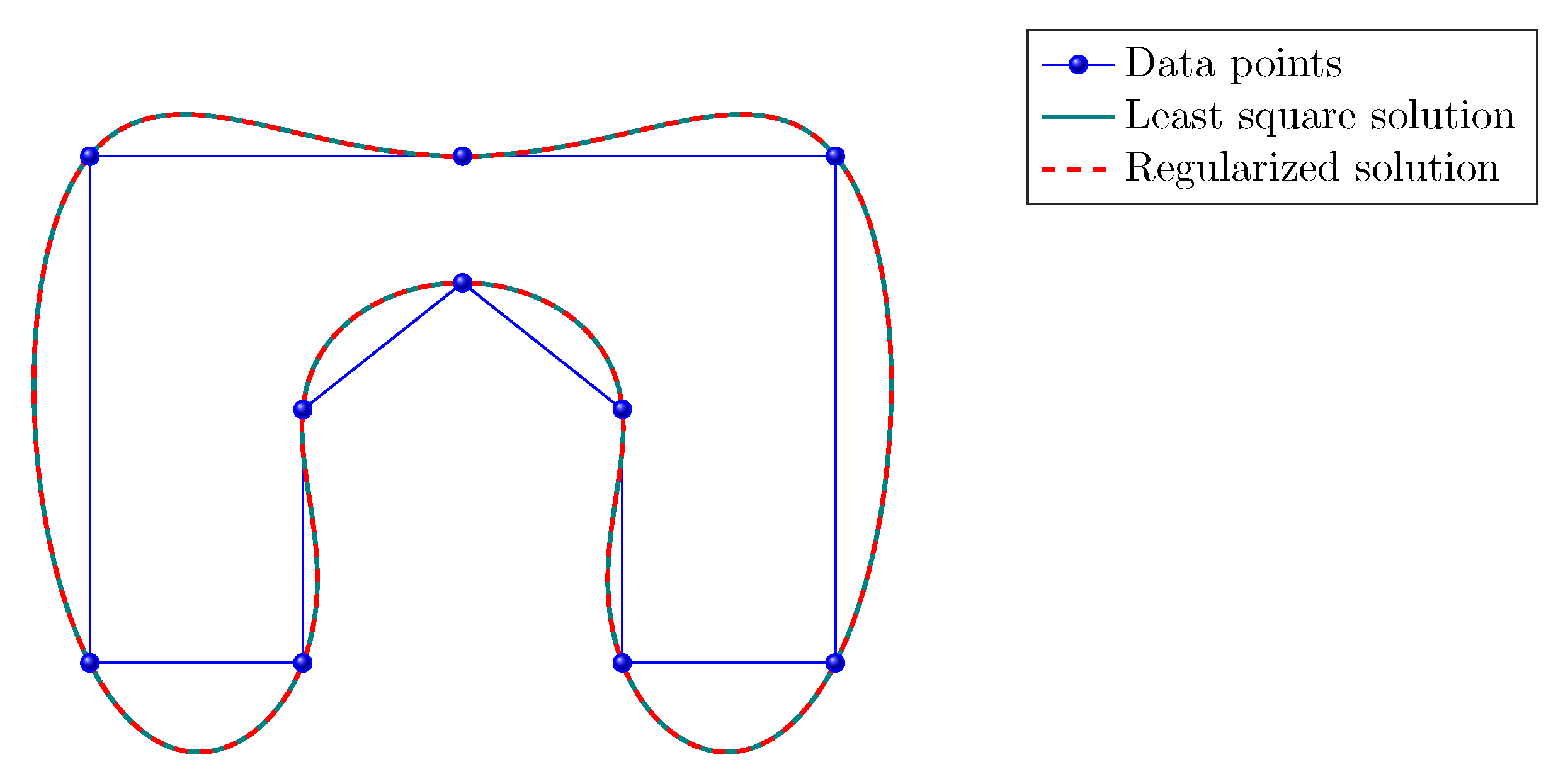
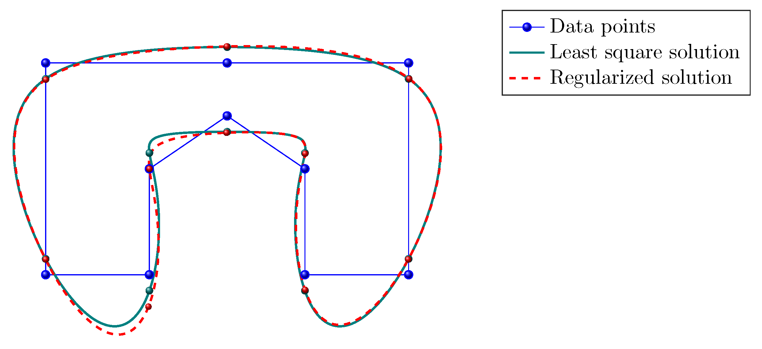
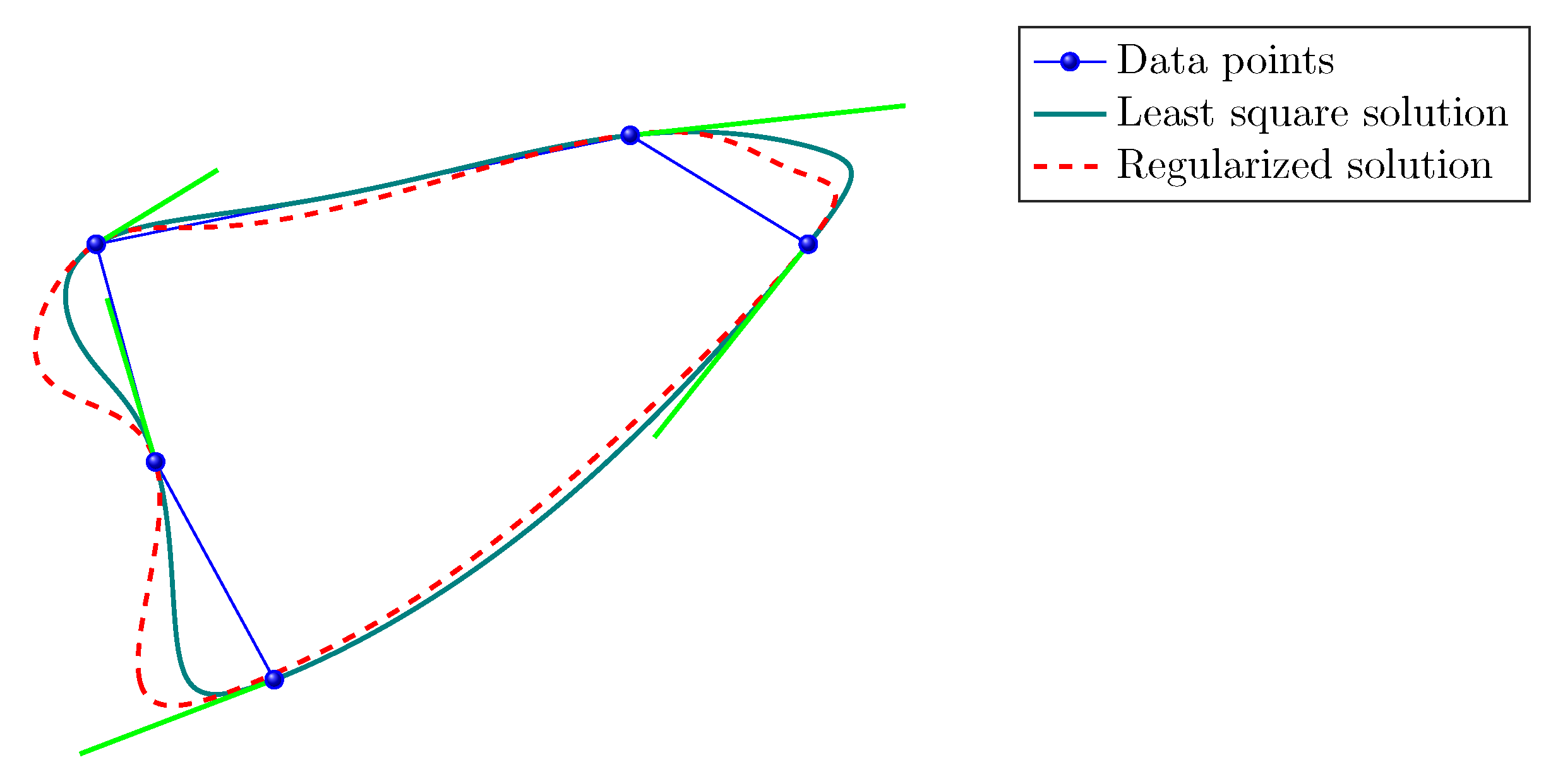
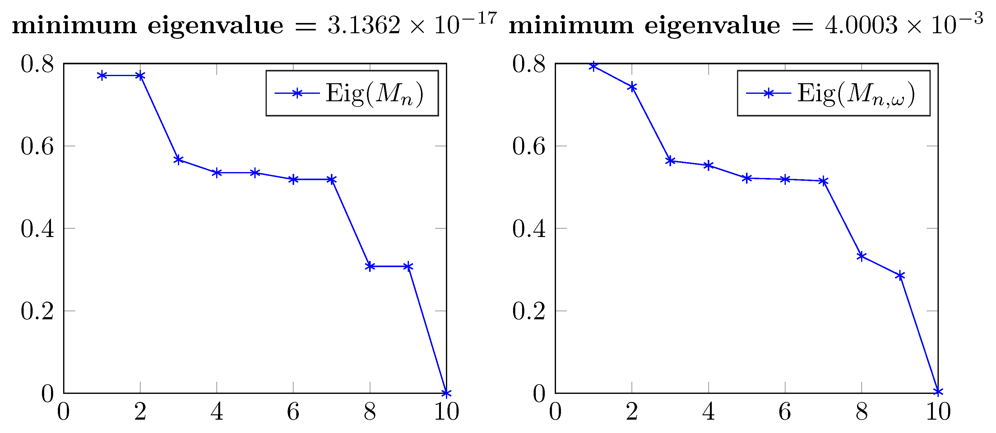
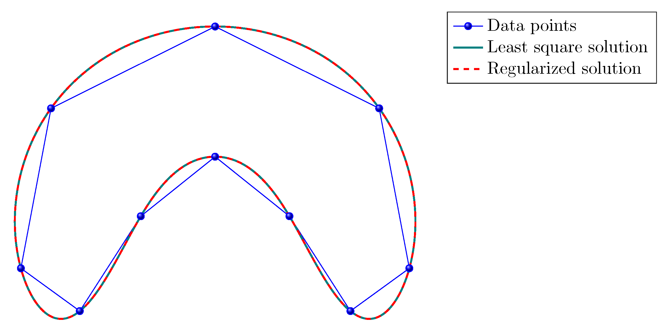
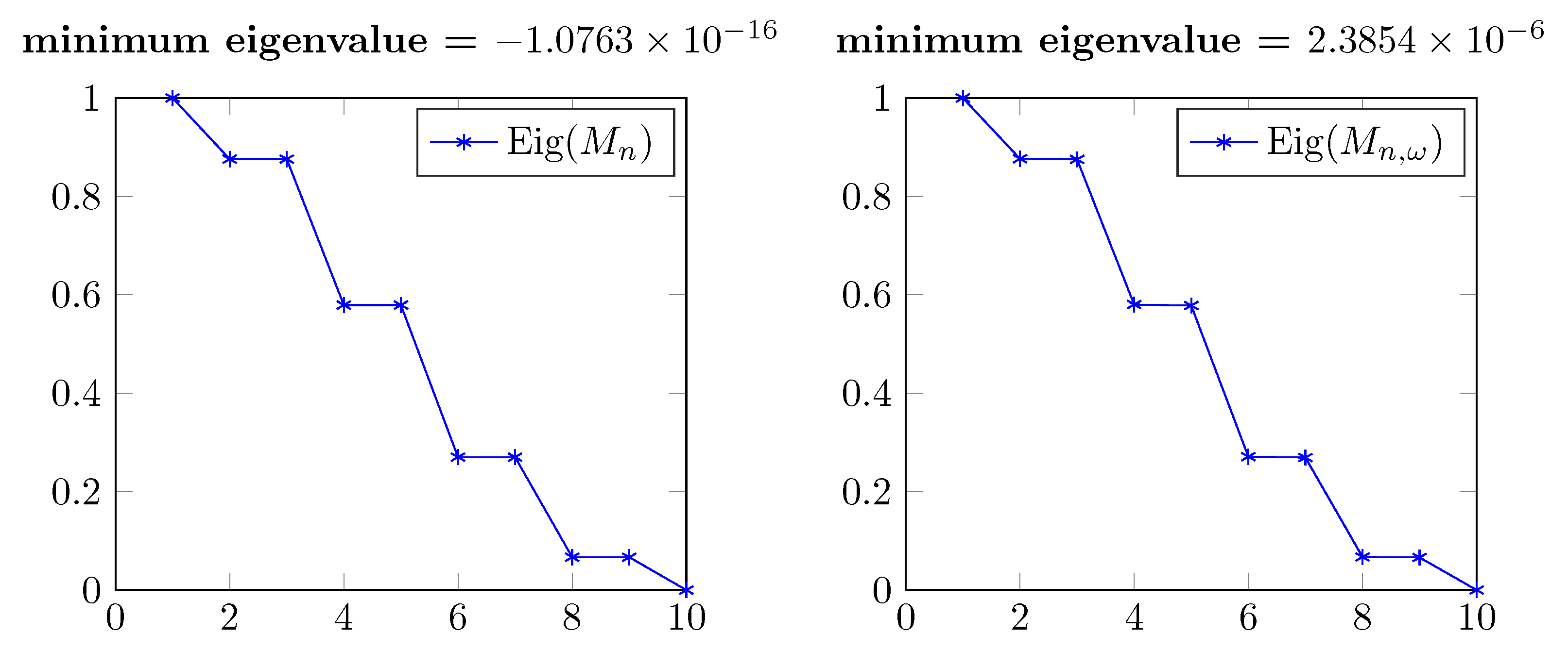
5.2. Our Regularizing Strategy

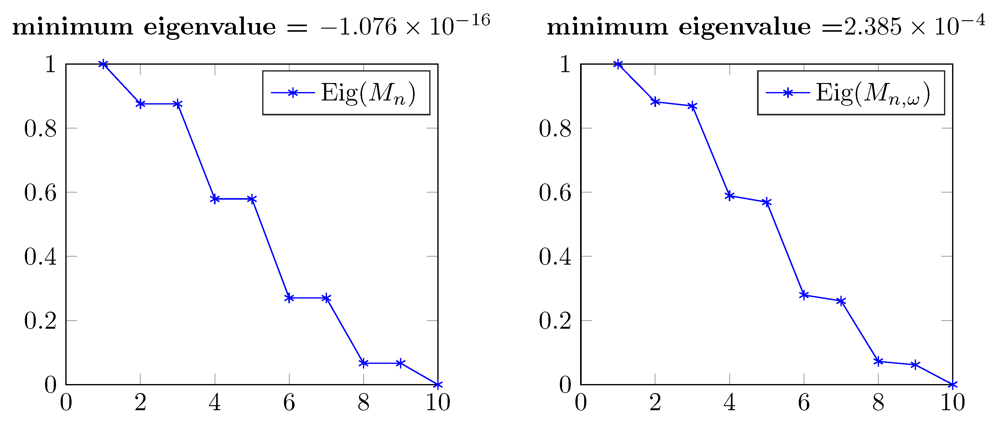
We have already observed that in some cases the matrix obtained by interpolating at integer parameters is singular and that sometimes the singularity cannot be avoided neither by a proper shift of the parameters. In those cases, independently of the interpolated points, the inverse of $M_n$ or ${\mathbf{M}}_n$ is not defined and an alternative solution has to be chosen. The first idea is using the pseudo-inverse of the matrix, providing a least-square solution [41]. Another approach is considering a regularization, which is an approximation of the ill-posed problem by a family of neighboring well-posed problems [40]. Among the regularization methods for solving an ill-posed problem whose discrete form is the linear system $Ax=b$ we mention the Tikhonov approach, which consists in solving the family of problems

$${\mathrm{argmin}}_x{∥Ax-b∥}^2+\lambda {∥Lx∥}^2,$$

depending on the regularization parameter $\lambda$. The latter controls the weight given to the residual norm and the regularization term. The optimal value for $\lambda$ can be chosen by discrepancy principle, generalized cross-validation, or the L-curve method [43]. The operator L, which can be taken as the identity operator or a differential operator (for instance, the first or second derivative operator), looks to alter the least square solution to enforce special features of the regularized approximations [40,43]. As a necessary condition it is required that $Ker\left(A\right)\cap Ker\left(L\right)=\left\{0\right\}$. This problem is equivalent to solve the normal equations $(A^{\top }A+\lambda L^{\top }L)x=A^{\top }b$ for each $\lambda$.

Since the quality of the obtained solution either by least-squares or Tikhonov regularization is not acceptable in many cases, in the following we study a new regularized problem depending on a parameter $\omega$ in which a (possibly block) $\omega$-circulant matrix replaces the original circulant coefficient matrix.

First we consider the basic interpolation case where $M_{n,\omega }$ is the $\omega$-circulant counterpart of $M_n$ with $\omega =\exp \left(\mathrm{i}\psi \right)$. By Remark 3, the eigenvalues of the new matrix $M_{n,\omega }$ are given by the standard uniform sampling of the function $b(\theta +\frac{\psi }{n})$. In this manner, the spectrum of $M_n$ is shifted. We observe that $M_n$ and $M_{n,\omega }$ are both singular if there exists at least two roots of $b\left(\theta \right)$ in the grid $\frac{2\pi \mathbb{N}}{n}\cap [0,2\pi ]$ with distance $\frac{\psi }{n}$.

If the latter condition is not satisfied, then the initial system $M_n{\mathbf{P}}^0={\mathbf{V}}^0$ is singular, while its perturbation $M_{n,\omega }{\mathbf{P}}^0={\mathbf{V}}^0$ has a unique, complex solution, even though the original problem is defined in the real domain. However, for $\psi$ small enough in modulus, the imaginary part of the solution becomes negligible and the perturbed system is close to the original one.

Secondly, we consider the interpolation of points and associated tangent vectors. The block (20) in the corresponding $\omega$-$(2\times 2)$-circulant matrix ${\mathbf{M}}_{n,\omega }$ is

$$\begin{array}{cc}\hfill {\left({\mathcal{L}}_{n,\omega }\right)}_{1,1}& =\sum _{j=0}^{\lceil \frac{p}{2}\rceil }{\mathit{B}}_j{\omega }^{j/n}+\sum _{j=1}^{\lceil \frac{p}{2}\rceil }{\mathit{B}}_{-j}{\omega }^{(n-j)/n}\hfill \\ \hfill & =\left[\begin{array}{cc}{\beta }_0^0& {\beta }_1^0\\ {\beta }_0^1& -{\beta }_1^1\end{array}\right]+\sum _{j=1}^{\lceil \frac{p}{2}\rceil }\left[\begin{array}{cc}{\beta }_{2j}^0& {\beta }_{2j-1}^0\\ {\beta }_{2j}^1& {\beta }_{2j-1}^1\end{array}\right]{\omega }^{j/n}+\sum _{j=1}^{\lceil \frac{p}{2}\rceil }\left[\begin{array}{cc}{\beta }_{2j}^0& {\beta }_{2j+1}^0\\ -{\beta }_{2j}^1& -{\beta }_{2j+1}^1\end{array}\right]{\omega }^{(n-j)/n}\hfill \\ \hfill & =\begin{array}{c}\hfill \left[\begin{array}{cc}{\displaystyle {\beta }_0^0+\sum _{j=1}^{\lceil \frac{p}{2}\rceil }{\beta }_{2j}^0\left({\omega }^{j/n}+{\omega }^{(n-j)/n}\right)}& {\displaystyle {\beta }_1^0\left(1+{\omega }^{(n-1)/n}\right)+\sum _{j=2}^{\lceil \frac{p}{2}\rceil }{\beta }_{2j-1}^0\left({\omega }^{j/n}+{\omega }^{(n-j)/n}\right)}\\ {\displaystyle \sum _{j=1}^{\lceil \frac{p}{2}\rceil }{\beta }_{2j}^1\left({\omega }^{j/n}-{\omega }^{(n-j)/n}\right)}& {\displaystyle {\beta }_1^1\left({\omega }^{1/n}-1\right)+\sum _{j=2}^{\lceil \frac{p}{2}\rceil }{\beta }_{2j-1}^1\left({\omega }^{j/n}-{\omega }^{(n-j)/n}\right)}\end{array}\right].\end{array}\hfill \end{array}$$

Then, ${\mathbf{M}}_{n,\omega }$ is not necessarily singular, even if ${\mathbf{M}}_n$ is, and we can solve ${\mathbf{M}}_{n,\omega }{\mathbf{P}}^0={\mathbf{U}}^{\left(2\right)}$ rather than (14). In this case, the structure of the symbol differs from (17) and (18).

Remark 4.

For the particular case of cubic B-spline curves, in Ref. [45] the point and tangent interpolation problem is solved by considering only the case of unitary tangents $V_j^1$, $j=0,\dots ,n-1$. Their proposal consists in a non-linear iterative method and convergence has not been proven.

6. Numerical Tests

In the present section we perform a few numerical tests in order to assess the quality of the solution obtained by adopting the $\omega$-circulant regularization, in the setting of a singular interpolation operator. In all the following examples we employ the J-spline family [38].

We denote by ${\widehat{\mathbf{P}}}^0$ and ${\widehat{\mathbf{P}}}_{\omega }^0$ the control point vectors obtained as $M_n^{†}{\mathbf{U}}^{\left(1\right)}$ (resp. ${\mathbf{M}}_n^{†}{\mathbf{U}}^{\left(2\right)}$ in the Hermite case) and $M_{n,\omega }^{†}{\mathbf{U}}^{\left(1\right)}$ (resp. ${\mathbf{M}}_{n,\omega }^{†}{\mathbf{U}}^{\left(2\right)}$ in the Hermite case), respectively. The pseudo-inverses $M_{n,\omega }^{†}$ and ${\mathbf{M}}_{n,\omega }^{†}$ are given by

$$(F_{n,\omega }\otimes I_d){\mathcal{L}}_{n,\omega }^{†}(F_{n,\omega }^{-1}\otimes I_d),\mathrm{with}{\left({\mathcal{L}}_{n,\omega }^{†}\right)}_k=\left\{\begin{array}{cc}\frac{1}{{\left({\mathcal{L}}_{n,\omega }\right)}_k}\hfill & ,\mathrm{if}{\left({\mathcal{L}}_{n,\omega }\right)}_k\ne 0,\hfill \\ 0\hfill & ,\mathrm{if}{\left({\mathcal{L}}_{n,\omega }\right)}_k=0,\hfill \end{array}\right.$$

with $d=1$ for $M_{n,\omega }^{†}$ and $d=2$ for ${\mathbf{M}}_{n,\omega }^{†}$, and where ${\left({\mathcal{L}}_{n,\omega }\right)}_k$ is the k-th diagonal element in (3). For $\omega =1$ we immediately get $M_n^{†}$ and ${\mathbf{M}}_n^{†}$.

We compare the subdivision curves generated from the control point vectors ${\widehat{\mathbf{P}}}^0$ and ${\widehat{\mathbf{P}}}_{\omega }^0$; firstly in terms of interpolation, which is the main goal. With this purpose, consider the residuals $M_n{\widehat{\mathbf{P}}}^0-{\mathbf{U}}^{\left(1\right)}$, ${\mathbf{M}}_n{\widehat{\mathbf{P}}}^0-{\mathbf{U}}^{\left(2\right)}$, $M_n{\widehat{\mathbf{P}}}_{\omega }^0-{\mathbf{U}}^{\left(1\right)}$ and ${\mathbf{M}}_n{\widehat{\mathbf{P}}}_{\omega }^0-{\mathbf{U}}^{\left(2\right)}$ which are vectors of points. Notice that the last two residuals are independent from the systems of equations $M_{n,\omega }{\widehat{\mathbf{P}}}_{\omega }^0={\mathbf{U}}^{\left(1\right)},$ ${\mathbf{M}}_{n,\omega }{\widehat{\mathbf{P}}}_{\omega }^0={\mathbf{U}}^{\left(2\right)},$ but they are related to the interpolation problems (10) and (14) with the regularized solution.

By reasoning in local terms, we choose the norms

$$∥M_n{\widehat{\mathbf{P}}}_{\omega }^0-{\mathbf{U}}^{\left(1\right)}∥,∥{\mathbf{M}}_n{\widehat{\mathbf{P}}}_{\omega }^0-{\mathbf{U}}^{\left(2\right)}∥$$

with $\parallel A\parallel :={\sup }_j{∥{\left(A\right)}_j∥}_2,$$A_j$ the j-row of matrix A and ${\parallel ·\parallel }_2$ the vector 2-norm. This way we measure how far the interpolated information in ${\mathbf{U}}^{\left(d\right)}$, $d=1,2$ is from the approximations in $M_{n,\omega }{\widehat{\mathbf{P}}}_{\omega }^0$, and ${\mathbf{M}}_{n,\omega }{\widehat{\mathbf{P}}}_{\omega }^0$ by the maximum distance.

On the other hand, reasoning in global terms we consider the relative error with Frobenius matrix norms

$$\frac{{∥M_n{\widehat{\mathbf{P}}}_{\omega }^0-{\mathbf{U}}^{\left(1\right)}∥}_{\mathrm{fro}}}{{∥{\mathbf{U}}^{\left(1\right)}∥}_{\mathrm{fro}}},\frac{{∥{\mathbf{M}}_n{\widehat{\mathbf{P}}}_{\omega }^0-{\mathbf{U}}^{\left(2\right)}∥}_{\mathrm{fro}}}{{∥{\mathbf{U}}^{\left(2\right)}∥}_{\mathrm{fro}}}.$$

In order to evaluate the quality of each curve, proper fairness measures could be used [46,47], penalizing artifacts such as loops (see Figure 5a).

In each figure, the curve obtained with the least square solution ${\widehat{\mathbf{P}}}^0$ is portrayed in solid green lines, while the one obtained with the regularized solution ${\widehat{\mathbf{P}}}_{\omega }^0$ is represented by dashed red lines.

The solution computed with the $\omega$-circulant matrix interpolates the given points even if a non singular matrix is used. Indeed, in Figure 6, where we set $\omega =\exp (5\times {10}^{-3}\mathrm{i})$, we only see one line because the two solutions ${\widehat{\mathbf{P}}}^0$ and ${\widehat{\mathbf{P}}}_{\omega }^0$ visually match. We get similar results with values of $\omega$ close to $\exp (5\times {10}^{-3}\mathrm{i})$. Hence, the quality of the interpolating solution is not affected by the perturbation.

Figure 6. Point interpolation with a quintic B-spline curve (that belongs to the J-spline family). Green solid line: least square solution. Red dashed line: regularized solution.

Applying a primal scheme with odd-symmetric mask as in (19), with a singular interpolation operator, the data points are not interpolated by the least square solution (see Figure 7). The spectrum of $M_n$ is perturbed considering a regularized solution and shifting the null eigenvalue as shown in Figure 8. As a result, the condition number is improved, but the approximation is not. In Figure 7 the results are shown for $\omega =\exp (5\times {10}^{-2}\mathrm{i})$. The residual norms are

$$\parallel M_n{\widehat{\mathbf{P}}}^0-{\mathbf{U}}^{\left(1\right)}\parallel =0.3,\parallel M_n{\widehat{\mathbf{P}}}_{\omega }^0-{\mathbf{U}}^{\left(1\right)}\parallel =0.6,$$

$$\frac{{∥M_n{\widehat{\mathbf{P}}}^0-{\mathbf{U}}^{\left(1\right)}∥}_{\mathrm{fro}}}{{∥{\mathbf{U}}^{\left(1\right)}∥}_{\mathrm{fro}}}=5.5\times {10}^{-2},\mathrm{and}\frac{{∥M_n{\widehat{\mathbf{P}}}_{\omega }^0-{\mathbf{U}}^{\left(1\right)}∥}_{\mathrm{fro}}}{{∥{\mathbf{U}}^{\left(1\right)}∥}_{\mathrm{fro}}}=6.0\times {10}^{-2}.$$

Figure 7. Point interpolation with a J-spline curve (19) with singular interpolation operator (that belongs to the J-spline family). Green solid line: least square solution. Red dashed line: regularized solution.

Figure 8. Eigenvalues of $M_n$ and $M_{n,\omega }$ (real part) in Figure 7.

It is worth noticing that the regularized curve is closer to the interpolation points, although this is not reflected in the norms.

In the block setting for point and tangent interpolation (see Figure 9) the situation is similar. Even though the spectrum of ${\mathbf{M}}_{n,\omega }$ is perturbed with respect to ${\mathbf{M}}_n$ and does not contain a null eigenvalue as the latter (see Figure 10), the solution is not improved; refer to Figure 9 in which $\omega =\exp (5\times {10}^{-1}\mathrm{i})$. We observe that the points are interpolated, but the tangent interpolation is less accurate. In this case the residual norms are

$$\parallel {\mathbf{M}}_n{\widehat{\mathbf{P}}}^0-{\mathbf{U}}^{\left(2\right)}\parallel =2.22\times {10}^{-15},\parallel {\mathbf{M}}_n{\widehat{\mathbf{P}}}_{\omega }^0-{\mathbf{U}}^{\left(2\right)}\parallel =1.15\times {10}^{-1},$$

$$\frac{{∥{\mathbf{M}}_n{\widehat{\mathbf{P}}}^0-{\mathbf{U}}^{\left(2\right)}∥}_{\mathrm{fro}}}{{∥{\mathbf{U}}^{\left(2\right)}∥}_{\mathrm{fro}}}=2.89\times {10}^{-16},\mathrm{and}\frac{{∥{\mathbf{M}}_n{\widehat{\mathbf{P}}}_{\omega }^0-{\mathbf{U}}^{\left(2\right)}∥}_{\mathrm{fro}}}{{∥{\mathbf{U}}^{\left(2\right)}∥}_{\mathrm{fro}}}=1.09\times {10}^{-2}.$$

Figure 9. Point and tangent vectors interpolation with a quintic B-spline curve (that belongs to the J-spline family). Green solid line: least square solution. Red dashed line: regularized solution.

Figure 10. Eigenvalues of ${\mathbf{M}}_n$ and ${\mathbf{M}}_{n,\omega }$ (real part) in Figure 9.

However, if we consider a known solution ${\mathbf{P}}^0$, we can generate ${\mathbf{U}}^{\left(1\right)}=M_n{\mathbf{P}}^0$ from the columns of $M_n$ and obtain, for a suitable parameter $\omega$, a solution that interpolates the points as accurately as the least square solution (see Figure 11 in which $\omega =\exp (5\times {10}^{-3}\mathrm{i})$), even though the spectra of $M_n$ and $M_{n,\omega }$ are different (see Figure 12).

Figure 11. Point interpolation with a J-spline curve (19) with a singular interpolation operator for a known solution. Green solid line: least square solution. Red dashed line: regularized solution.

Figure 12. Eigenvalues of $M_n$ and $M_{n,\omega }$ (real part) in Figure 11.

7. Conclusions

In the present work we explored two distinct applications of $\omega$-circulant matrices.

After a brief introduction of this matrix algebra and its fundamental properties, we first described their role in the parallel solution and preconditioning of (block) triangular linear systems of Toeplitz type. We recalled an efficient classical algorithm, which relies on the well-known diagonalization of $\omega$-circulants through the FFT, and studied the stability issue, which needs special attention due to the fact that the condition number of the fast transform strongly depends on the parameter $\omega$.

Then we analyzed subdivision schemes, for which a few questions remain open.

Indeed, the interpolation of points and tangent vectors with scalar subdivision schemes as inverse problem may lead to a system of equations with a singular matrix. We proposed as a first possible solution to change the common approach of interpolating at integer parameters in dependence of the symmetry of the subdivision mask. With this solution we avoid the presence of a singular matrix in the model and we still benefit from the Fourier factorization of a non-singular circulant or block-circulant matrix.

In some cases it is not possible to avoid the singularity while keeping the symmetry of the stencil. In such situations we considered the solution obtained by the means of least square solution and related $\omega$-circulant regolarization for the interpolation problem. More in detail, owing to the singular character of the matrix in the interpolation setting, difficulties are overcome by perturbing the spectrum, by taking into consideration its $\omega$-circulant counterpart.

As observed in the numerical experiments, the $\omega$-regularization approach is not sufficient for solving the problem. When the original is singular, the $\omega$-perturbation is well conditioned, but the interpolation condition is not represented exactly and the latter affects the approximation quality. However, the numerical solution stemming from the $\omega$-circulant linear system interpolates the data points at least in some cases where the solution is known.

A further open problem is the study of the solution Sol($\exp \left(\mathrm{i}\psi \right)$: in this setting, we would like to explore the existence of an asymptotic expansion of the form

$$\mathrm{Sol}\left(\exp \left(\mathrm{i}\psi \right)\right)=\mathrm{Sol}+c_1\psi +c_2{\psi }^2+c_3{\psi }^3+\cdots ,$$

when a small parameter $\psi$ is considered.

An expansion of the latter type would open the door to simple and cheap extrapolation procedures for the computation of very precise solutions. Preliminary numerical have been performed and are encouraging. We are convinced that this research line is worth to be investigated in future steps.

References

- Garoni, C.; Serra-Capizzano, S. Generalized Locally Toeplitz Sequences: Theory and Applications, Vol. I; Springer: Cham, Switzerland, 2017. [Google Scholar]
- Ng, M.K. Iterative Methods for Toeplitz Systems. Numerical Mathematics and Scientific Computation; Oxford University Press: New York, NY, USA, 2004. [Google Scholar]
- Aricò, A.; Serra-Capizzano, S.; Tasche, M. Fast and numerically stable algorithms for discrete Hartley transforms and applications to preconditioning. Commun. Inf. Syst. 2005, 5, 21–68. [Google Scholar] [CrossRef]
- Hansen, P.C.; Nagy, J.G.; O’Leary, D.P. Deblurring images. Matrices, spectra, and filtering. In Fundamentals of Algorithms; Society for Industrial and Applied Mathematics: Philadelphia, PA, USA, 2006; Volume 3. [Google Scholar]
- Kailath, T.; Olshevsky, V. Displacement structure approach to discrete-trigonometric-transform based preconditioners of G. Strang type and of T. Chan type. Toeplitz matrices: Structures, algorithms and applications. (Cortona, 1996). Calcolo 1998, 33, 191–208. [Google Scholar] [CrossRef]
- Serra-Capizzano, S. A Korovkin-type theory for finite Toeplitz operators via matrix algebras. Numer. Math. 1999, 82, 117–142. [Google Scholar] [CrossRef]
- Davis, P. Circulant Matrices; John Wiley and Sons: Hoboken, NJ, USA, 1979. [Google Scholar]
- Bini, D. Matrix structures in parallel matrix computations. Calcolo 1988, 25, 37–51. [Google Scholar] [CrossRef]
- Chan, R.H.F.; Jin, X.Q. An introduction to iterative Toeplitz solvers. In Fundamentals of Algorithms; Society for Industrial and Applied Mathematics (SIAM): Philadelphia, PA, USA, 2007; Volume 5. [Google Scholar]
- Chan, R.H.; Ng, M.K. Conjugate gradient methods for Toeplitz systems. SIAM Rev. 1996, 38, 427–482. [Google Scholar] [CrossRef]
- Chan, T.F.; Elman, H.C. Fourier analysis of iterative methods for elliptic problems. SIAM Rev. 1989, 31, 20–49. [Google Scholar] [CrossRef]
- Huckle, T. A note on skewcirculant preconditioners for elliptic problems. Numer. Algorithms 1992, 2, 279–286. [Google Scholar] [CrossRef]
- Huckle, T. Thomas Circulant and skewcirculant matrices for solving Toeplitz matrix problems. Iterative methods in numerical linear algebra (Copper Mountain, CO, 1990). SIAM J. Matrix Anal. Appl. 1992, 13, 767–777. [Google Scholar] [CrossRef]
- Serra-Capizzano, S. The GLT class as a generalized Fourier analysis and applications. Linear Algebra Appl. 2006, 419, 180–233. [Google Scholar] [CrossRef]
- Loan, C.V. Computational frameworks for the fast Fourier transform. In Frontiers in Applied Mathematics; Society for Industrial and Applied Mathematics (SIAM): Philadelphia, PA, USA, 1992; Volume 10. [Google Scholar]
- Aricò, A.; Donatelli, M.; Serra-Capizzano, S. V-cycle optimal convergence for certain (multilevel) structured linear systems. SIAM J. Matrix Anal. Appl. 2004, 26, 186–214. [Google Scholar] [CrossRef]
- Bertaccini, D.; Ng, M.K. Block ω-circulant preconditioners for the systems of differential equations. Calcolo 2003, 40, 71–90. [Google Scholar] [CrossRef]
- Serra-Capizzano, S.; Tablino-Possio, C. Multigrid methods for multilevel circulant matrices. SIAM J. Sci. Comput. 2004, 26, 55–85. [Google Scholar] [CrossRef]
- Bini, D. Parallel solutions of certain Toeplitz linear systems. SIAM J. Comput. 1984, 13, 268–276. [Google Scholar] [CrossRef]
- Cline, R.E.; Plemmons, R.J.; Worm, G. Generalized inverses of certain Toeplitz matrices. Linear Algebra Its Appl. 1974, 8, 25–33. [Google Scholar] [CrossRef]
- Liu, J.; Wu, S.L. A fast block α-circulant preconditioner for all-at-once systems from wave equations. SIAM J. Matrix Anal. Appl. 2020, 41, 1912–1943. [Google Scholar] [CrossRef]
- Hon, S.; Serra-Capizzano, S. A block Toeplitz preconditioner for all-at-once systems from linear wave equations. Electron. Trans. Numer. Anal. 2023, 58, 177–195. [Google Scholar] [CrossRef]
- Danieli, F.; Wathen, A.J. All-at-once solution of linear wave equations. (English summary). Numer. Linear Algebra Appl. 2021, 28, 16. [Google Scholar] [CrossRef]
- Gander, M.J.; Halpern, L.; Rannou, J.; Ryan, J. A direct time parallel solver by diagonalization for the wave equation. SIAM J. Sci. Comput. 2019, 41, A220–A245. [Google Scholar] [CrossRef]
- Gander, M.J.; Wu, S.L. A diagonalization-based parareal algorithm for dissipative and wave propagation problems. SIAM J. Numer. Anal. 2020, 58, 2981–3009. [Google Scholar] [CrossRef]
- Soszyńska, M.; Richter, T. Adaptive time-step control for a monolithic multirate scheme coupling the heat and wave equation. BIT 2021, 61, 1367–1396. [Google Scholar] [CrossRef]
- Bertaccini, D.; Durastante, F. Limited memory block preconditioners for fast solution of fractional partial differential equations. J. Sci. Comput. 2018, 77, 950–970. [Google Scholar] [CrossRef]
- Jiang, Y.; Liu, J. Fast parallel-in-time quasi-boundary value methods for backward heat conduction problems. Appl. Numer. Math. 2023, 184, 325–339. [Google Scholar] [CrossRef]
- Andersson, L.E.; Stewart, N.F. Introduction to the Mathematics of Subdivision Surfaces; Society for Industrial and Applied Mathematics: Philadelphia, PA, USA, 2010. [Google Scholar]
- Dyn, N. Linear and Nonlinear Subdivision Schemes in Geometric Modeling; School of Mathematical Sciences, Tel Aviv University: Tel Aviv, Israel, 2008. [Google Scholar]
- Dyn, N.; Levin, D. Subdivision schemes in geometric modelling. Acta Numer. 2002, 11, 73–144. [Google Scholar] [CrossRef]
- Dyn, N.; Levin, D.; Gregory, J.A. A 4-point interpolatory subdivision scheme for curve design. Comput. Aided Geom. Des. 1987, 4, 257–268. [Google Scholar] [CrossRef]
- Sabin, M. Analysis and Design of Univariate Subdivision Schemes; Springer: Berlin/Heidelberg, Germany, 2010. [Google Scholar]
- Chui, C.; de Villiers, J. Wavelet Subdivision Methods: Gems for Rendering Curves and Surfaces; CRC Press: Boca Raton, FL, USA, 2010. [Google Scholar]
- Schaefer, S.; Warren, J. Exact evaluation of limits and tangents for non-polynomial subdivision schemes. Comput. Aided Geom. Des. 2008, 25, 607–620. [Google Scholar] [CrossRef]
- Daubechies, I.; Guskov, I.; Sweldens, W. Commutation for irregular subdivision. Constr. Approx. 2001, 17, 479–514. [Google Scholar] [CrossRef]
- Dyn, N.; Gregory, J.A.; Levin, D. Analysis of uniform binary subdivision schemes for curve design. Constr. Approx. 1991, 7, 127–147. [Google Scholar] [CrossRef]
- Rossignac, J.; Schaefer, S. J-splines. Comput. Aided Des. 2008, 40, 1024–1032. [Google Scholar] [CrossRef]
- Dyn, N.; Floater, M.S.; Hormann, K. A C2 four-point subdivision scheme with fourth order accuracy and its extensions. In Mathematical Methods for Curves and Surfaces: TROMSØ 2004, Modern Methods in Mathematics; Nashboro Press: Brentwood, TN, USA, 2005; pp. 145–156. [Google Scholar]
- Engl, H.W.; Hanke, M.; Neubauer, A. Regularization of Inverse Problems; Springer: New York, NY, USA, 1996. [Google Scholar]
- Hoppe, H.; DeRose, T.; Duchamp, T.; Halstead, M.; Jin, H.; McDonald, J.; Schweitzer, J.; Stuetzle, W. Piecewise smooth surface reconstruction. In Proceedings of the 21st Annual Conference on Computer Graphics and Interactive Techniques, Orlando, FL, USA, 24–29 July 1994; pp. 295–302. [Google Scholar]
- Halstead, M.A.; Kass, M.; DeRose, T. Efficient, fair interpolation using Catmull-Clark surfaces. In Proceedings of the 20th Annual Conference on Computer Graphics and Interactive Techniques, Anaheim, CA, USA, 2–6 August 1993; pp. 35–44. [Google Scholar]
- Hansen, P.C. Rank-Deficient and Discrete Ill-Posed Problems: Numerical Aspects of Linear Inversion; Society for Industrial and Applied Mathematics: Philadelphia, PA, USA, 1999. [Google Scholar]
- Plonka, G. An efficient algorithm for periodic Hermite spline interpolation with shifted nodes. Numer. Algorithms 1993, 5, 51–62. [Google Scholar] [CrossRef]
- Okaniwa, S.; Nasri, A.; Lin, H.; Abbas, A.; Kineri, Y.; Maekawa, T. Uniform B-spline curve interpolation with prescribed tangent and curvature vectors. IEEE Trans. Vis. Comput. Graph. 2012, 18, 1474–1487. [Google Scholar] [CrossRef]
- Albrecht, G. Invariante Gütekriterien im Kurvendesign–Einige neuere Entwicklungen. Effiziente Methoden der Geometrischen Modellierung und der Wissenschaftlichen Visualisierung; Springer: Berlin/Heidelberg, Germany, 1999; pp. 134–148. [Google Scholar]
- Veltkamp, R.C.; Wesselink, W. Modeling 3D curves of minimal energy. Comput. Graph. Forum 1995, 14, 97–110. [Google Scholar] [CrossRef]
Disclaimer/Publisher’s Note: The statements, opinions and data contained in all publications are solely those of the individual author(s) and contributor(s) and not of MDPI and/or the editor(s). MDPI and/or the editor(s) disclaim responsibility for any injury to people or property resulting from any ideas, methods, instructions or products referred to in the content. |
© 2023 by the authors. Licensee MDPI, Basel, Switzerland. This article is an open access article distributed under the terms and conditions of the Creative Commons Attribution (CC BY) license (https://creativecommons.org/licenses/by/4.0/).