Algorithm for Approximate Solving of a Nonlinear Boundary Value Problem for Generalized Proportional Caputo Fractional Differential Equations

Abstract

In this paper an algorithm for approximate solving of a boundary value problem for a nonlinear differential equation with a special type of fractional derivative is suggested. This derivative is called a generalized proportional Caputo fractional derivative. The new algorithm is based on the application of the monotone-iterative technique combined with the method of lower and upper solutions. In connection with this, initially, the linear fractional differential equation with a boundary condition is studied, and its explicit solution is obtained. An appropriate integral fractional operator for the nonlinear problem is constructed and it is used to define the mild solutions, upper mild solutions and lower mild solutions of the given problem. Based on this integral operator we suggest a scheme for obtaining two monotone sequences of successive approximations. Both sequences consist of lower mild solutions and lower upper solutions of the studied problem, respectively. The monotonic uniform convergence of both sequences to mild solutions is proved. The algorithm is computerized and applied to a particular example to illustrate the theoretical investigations.

1. Introduction

Fractional derivatives of any type are adequate models of the dynamics of many phenomena and process in engineering, population dynamics, ecology, etc. In the literature there are several types of fractional derivatives such as Caputo fractional derivative, Riemann–Liouville fractional derivative [1,2], proportional fractional derivative with respect to other functions [3], Caputo–Fabrizio fractional derivative [4] and ABC fractional derivative [5]. Some of the basic types of fractional derivatives are applied to models such as the fractional models of gas dynamics [6], the fractional model in the dynamics of particles [7], the computer virus fractional-order model [8] and the fractional models in geo-hydrology [9].

In the last decade the generalized proportional fractional derivative of Caputo type (PFD) was introduced [10,11] and applied to differential equations. Several qualitative properties of the solutions of differential equations with PFD are well studied. We could mention the existence results [12], the existence and Ulam-type stability [13,14] results, some numerical solutions [15] and explicit solutions in the cases with and without impulses [16].

Note that when PFD is applied to nonlinear differential equations it is very difficult to obtain the solution in an explicit form. It leads to more complicated practical application and investigation of the properties of the solutions. It requires the use of numerical and approximate methods for obtaining the solutions of the studied differential equations with initial and boundary conditions. One of the approximate methods giving solutions as a limit of a sequence of functions is the monotone iterative method. It is theoretically proved and applied to initial value problems for various types of fractional differential equations such as the Caputo fractional evolution problem [17], fractional-order neutral differential equations [18] and Riemann–Liouville fractional differential equations [19]. These method is also successfully applied to some boundary value problems for Riemann–Liouville fractional differential equations [20,21,22,23] and for the $\psi$-Caputo fractional differential equation [24]. To the best of our knowledge, the monotone-iterative technique is not applied to a nonlinear boundary value problem for differential equations with PFD.

The aim of this paper is to present a new algorithm for approximate solving of a nonlinear boundary value problem (BVP) for a scalar nonlinear differential equation with PFD of Caputo type. A new type of integral fractional operator is suggested and it is used to define lower and upper mild solutions of the studied problem. Based on this integral fractional operator two sequences of successive approximations are constructed and their convergence to the mild solution of the studied problem is proved. The proposed scheme is based on the monotone-iterative technique. Initially, the BVP for the linear differential equation with PFD is studied and its explicit solution is given. The suggested scheme for approximate solutions is computerized and applied to a particular example.

The paper is organized in the following manner. In Section 2 well-known literature definitions, lemmas and propositions for PGDs of Caputo type are given. The main results are presented in Section 3. In Section 3.1, the initial value problem for a linear differential equation with PFD of Caputo type is considered and its explicit solution is provided. Then mild solutions, mild lower and upper solutions of the studied nonlinear problem are defined. In Section 3.2 the monotone-iterative technique is applied to the BVP for nonlinear differential equations with PDE of Caputo type. Theoretically some claims about the sequences of successive approximations are proved. In Section 4 the new algorithm is briefly described. In Section 5 the suggested algorithm for successive approximations is illustrated on an example by the application of the appropriate computer program which ideas are presented in Section 6. Some concluding remarks are given in the Section 7.

2. Preliminary Notes

In this paper we apply the generalized proportional fractional derivative of Caputo type to differential equations. For better understanding of the results we will give some known-in-the-literature definitions and results about this type of derivative.

$$\begin{array}{cc}& \left({}_0{\mathcal{I}}^{\gamma ,\xi }y\right)\left(\sigma \right)=\frac{1}{{\xi }^{\gamma }\Gamma \left(\gamma \right)}{\int }_0^{\sigma }{e}^{\frac{\xi -1}{\xi }\left(\sigma -\tau \right)}{\left(\sigma -\tau \right)}^{\gamma -1}y\left(\tau \right)d\tau ,\sigma \in (0,a],\gamma \ge 0,\xi \in (0,1],\hfill \end{array}$$

Suppose we have a point $a\in R:a<\infty$ and the function $y:[0,a]\to ℝ$.

The generalized proportional fractional integral (GPFI) of the function y is defined by [10,11].

$$\begin{array}{cc}& \left({}_0{\mathcal{I}}^{\gamma ,\xi }y\right)\left(\sigma \right)=\frac{1}{{\xi }^{\gamma }\Gamma \left(\gamma \right)}{\int }_0^{\sigma }{e}^{\frac{\xi -1}{\xi }\left(\sigma -\tau \right)}{\left(\sigma -\tau \right)}^{\gamma -1}y\left(\tau \right)d\tau ,\sigma \in (0,a],\gamma \ge 0,\xi \in (0,1],\hfill \end{array}$$

and the generalized proportional Caputo fractional derivative (PFD) of function y is defined by the equality [10,11].

$$\begin{array}{cc}& \left({}_0^C{\mathcal{D}}^{\gamma ,\xi }y\right)\left(\sigma \right)=\frac{1-\xi }{{\xi }^{1-\gamma }\Gamma (1-\gamma )}{\int }_0^{\sigma }{e}^{\frac{\xi -1}{\xi }\left(\sigma -\tau \right)}{\left(\sigma -\tau \right)}^{-\gamma }y\left(\tau \right)d\tau \hfill \\ & +\frac{{\xi }^{\gamma }}{\Gamma (1-\gamma )}{\int }_0^{\sigma }{e}^{\frac{\xi -1}{\xi }\left(\sigma -\tau \right)}{\left(\sigma -\tau \right)}^{-\gamma }{y}^{\prime }\left(\tau \right)d\tau ,\sigma \in (0,a],\gamma \in (0,1),\xi \in (0,1].\hfill \end{array}$$

(1)

The defined above PFD and GPFI are generalizations of the classical Caputo fractional derivative of order $\gamma \in (0,1)$ and Riemann–Liouville fractional integral of order $\gamma >0$, respectively (for more information, see, for example, the classical book [25]).

Remark 1 

(see [10] [Remark 3.2]). The relations $\left({}_0^C{\mathcal{D}}^{\gamma ,\xi }K\right)\left(\sigma \right)\ne 0$ with $K\ne 0$ being a constant and $\left({}_0^C{\mathcal{D}}^{\gamma ,\xi }{e}^{\frac{\xi -1}{\xi }(.)}\right)\left(\sigma \right)=0$ for $\sigma >0$ hold. Note that these properties of PFD are totally different than the well known properties of ordinary derivatives of a constant. These properties, combined with the memory properties of PFD, gives us additionally better opportunities in the application for modeling real world phenomena.

Lemma 1 

(Proposition 5.2 [10]). For $\xi \in (0,1]$ and $\gamma \in (0,1)$ we have the equality for PFD

$${}_0^C{\mathcal{D}}^{\gamma ,\xi }(e^{\frac{\xi -1}{\xi }t}{t}^{\beta -1})\left(\sigma \right)=\frac{{\xi }^{\gamma }\Gamma \left(\beta \right)}{\Gamma (\beta -\gamma )}{e}^{\frac{\xi -1}{\xi }\sigma }{\sigma }^{\beta -1-\gamma },\beta >0.$$

Lemma 2 

(Lemma 5 [26]). If we have a function $\phi \in C\left(\right[0,a],ℝ)$, and there exists a number $\eta \in (0,a):\phi \left(\eta \right)=0$, and $\phi \left(\sigma \right)<0$ for $0\le \sigma <\eta .$ Then if there exists $\left({}_0^c{\mathcal{D}}^{\gamma ,\xi }\phi \right)\left(\eta \right)$, then the inequality $\left({}_0^c{\mathcal{D}}^{\gamma ,\xi }\phi \right)\left(\eta \right)>0$ holds.

Consider the classes of functions:

$$\begin{array}{cc}& C^{\gamma ,\xi }[0,a]=\{\phi :[0,a]\to ℝ:\left({}_0^C{\mathcal{D}}^{\gamma ,\xi }\phi \right)\left(\sigma \right)\mathrm{exists} \mathrm{for} \mathrm{all}\sigma \in (0,a]\},\hfill \\ & I^{\gamma ,\xi }[0,a]=\{\phi :[0,a]\to ℝ:\left({}_0{\mathcal{I}}^{\gamma ,\xi }\phi \right)\left(\sigma \right)\mathrm{exists} \mathrm{for} \mathrm{all} \sigma \in (0,a]\}.\hfill \end{array}$$

For any function $\phi \in C^{\gamma ,\xi }[0,a]$ and ${}_0{\mathcal{D}}^{\gamma ,\xi }\phi (.)\in I^{\gamma ,\xi }[0,a]$ with $\xi \in (0,1],\gamma \in (0,1)$ we have the following result:

Proposition 1 

(Theorem 5.3 [10]). Let $\xi \in (0,1]$ and $\gamma \in (0,1)$. Then the equality

$$\left({}_0{\mathcal{I}}^{\gamma ,\xi }\left({}_0^C{\mathcal{D}}^{\gamma ,\xi }\phi \right)\right)\left(\sigma \right)=\phi \left(\sigma \right)-\phi \left(0\right)e^{\frac{\xi -1}{\xi }\sigma },\sigma \in (0,a]$$

holds.

For any function $\phi \in I^{\gamma ,\xi }[0,a]$ and ${}_0{\mathcal{I}}^{\gamma ,\xi }\phi (.)\in C^{\gamma ,\xi }[0,a]$ with $\xi \in (0,1],\gamma \in (0,1)$ we have the following result:

Proposition 2 

([10]). Let $\gamma \in (0,1)$ and $\gamma \in (0,1)$. Then

$$\left({}_0^C{\mathcal{D}}^{\gamma ,\xi }\left({}_0{\mathcal{I}}^{\gamma ,\xi }\phi \right)\right)\left(\sigma \right)=\phi \left(\sigma \right),\sigma \in (0,a].$$

3. Main Theoretical Results

3.1. Mild Solutions of the Generalized Proportional Caputo Fractional Differential Equation

First, we will investigate the linear case and we will provide an explicit solution to the corresponding initial value problem.

Consider the linear scalar fractional differential equation with the PFD and an initial condition (IVPL)

$$\begin{array}{cc}\hfill & \left({}_0^C{\mathcal{D}}^{\gamma ,\xi }\phi \right)\left(\sigma \right)=-\lambda \phi \left(t\right)+\Phi \left(t\right),\sigma \in (0,a],\hfill \\ \hfill & \phi \left(0\right)={\phi }_0\hfill \end{array}$$

(2)

where ${\phi }_0\in ℝ$, $\xi \in (0,1]$, $\gamma \in (0,1)$, $\lambda \in ℝ$ is a constant, $\Phi \in C\left(\right[0,a],ℝ)$.

Lemma 3 

(see Example 5.7 [10]). Let the function $\Phi \in I^{\gamma ,\xi }[0,a]$. Then the IVPL (2) has a unique solution $\phi \in C^{\gamma ,\xi }[0,a]$ given by the equality

$$\begin{array}{cc}\hfill & \phi \left(\sigma \right)={\phi }_0{e}^{(\xi -1)\frac{\sigma }{\xi }}{E}_{\gamma }\left(-\lambda {\left(\frac{\sigma }{\xi }\right)}^{\gamma }\right)\hfill \\ \hfill & +\frac{1}{{\xi }^{\gamma }\Gamma \left(\gamma \right)}{\int }_0^{\sigma }{(\sigma -\tau )}^{\gamma -1}{e}^{(\xi -1)\left(\frac{\sigma -\tau }{\xi }\right)}{E}_{\gamma ,\gamma }(-\lambda {\left(\frac{\sigma -\tau }{\xi }\right)}^{\gamma })\Phi \left(\tau \right)d\tau ,\sigma \in (0,a],\hfill \end{array}$$

(3)

where the notations $E_{\gamma }(.)$ and $E_{\gamma ,\gamma }(.)$ are used for the Mittag-Leffler functions with one and two parameters, respectively.

Consider the nonlinear scalar differential equation with PFD and a nonlinear boundary condition (GPDE):

$$\begin{array}{cc}& \left({}_0^C{\mathcal{D}}^{\gamma ,\xi }y\right)\left(\sigma \right)=\vartheta \left(\sigma ,y\left(\sigma \right)\right),\sigma \in (0,a],\hfill \\ & \Delta \left(y\left(0\right),y\left(a\right)\right)=0,\hfill \end{array}$$

(4)

where $\xi \in (0,1],\gamma \in (0,1)$, $\vartheta :[0,a]\times \mathbb{R}\to \mathbb{R}$ and $\Delta :\mathbb{R}\times \mathbb{R}\to \mathbb{R}$.

Remark 2.

Any function $y\in C^{\gamma ,\xi }[0,a]$ satisfying both equalities (4) is called a solution of GPDE (4).

Let $\lambda ,\mu >0$ be constants (to be determined later). For any solution $y\in C^{\gamma ,\xi }[0,T]$ of GPDE (4) we define ${\psi }_y=y\left(0\right)-\frac{1}{\mu }\Delta (y\left(0\right),y\left(a\right))$. Then GPDE (4) can be equivalently written in the form

$$\begin{array}{cc}& \left({}_0^C{\mathcal{D}}^{\gamma ,\xi }y\right)\left(\sigma \right)=-\lambda y\left(\sigma \right)+\mathrm{Y}\left(\sigma ,y\left(\sigma \right)\right),\sigma \in [0,a],\hfill \\ & y\left(0\right)={\psi }_y,\hfill \end{array}$$

(5)

where

$$\mathrm{Y}\left(\sigma ,y\right)=\vartheta \left(\sigma ,y\right)+\lambda y,y\in ℝ,\sigma \in (0,a].$$

(6)

Note the problem (5) is an initial value problem for the nonlinear differential equation with PFD. Based on the explicit solution (3) of the IVPL (2) we will define a mild solution of (5) and its equivalent GPDE (4).

Define the integral fractional operator $\Omega :C[0,a]\to C[0,a]$ by

$$\begin{array}{cc}& (\Omega \phi )\left(\sigma \right)=\left(\phi \left(0\right)-\frac{1}{\mu }\Delta (\phi \left(0\right),\phi \left(a\right))\right)e^{(\xi -1)\frac{\sigma }{\xi }}{E}_{\gamma }(-\lambda {\left(\frac{\sigma }{\xi }\right)}^{\gamma })\hfill \\ & +\frac{1}{{\xi }^{\gamma }\Gamma \left(\gamma \right)}{\int }_0^{\sigma }{(\sigma -\tau )}^{\gamma -1}{e}^{(\xi -1)\left(\frac{\sigma -\tau }{\xi }\right)}{E}_{\gamma ,\gamma }(-\lambda {\left(\frac{\sigma -\tau }{\xi }\right)}^{\gamma })\left(\vartheta (\tau ,\phi (\tau \left)\right)+\lambda \phi \left(\tau \right)\right)d\tau ,\hfill \\ & \sigma \in [0,a],\hfill \end{array}$$

(7)

where $\lambda ,\mu$ are given positive constants (we will define them later).

The mild solutions of fractional differential equations play an important role in the study of various qualitative properties of the solutions. Mild solutions are defined by the application of an appropriate integral operator deeply connected with the studied fractional differential equation (see, for example, Definition 3.1. Ref. [27] for fractional neutral evolution equations, Ref. [28] for fractional evolution equation, Ref. [29] for Caputo–Hadamard fractional differential equations).

Definition 1.

Any fixed point $\phi \in C[0,a]$ (if any) of the operator Ω is called a mild solution of GPDE (4).

Theorem 1.

Let for any function $\phi \in C^{\gamma ,\xi }[0,a]$ the function $f(.,\phi (.))\in I^{\gamma ,\xi }[0,a]$. Then any solution $x\in C^{\gamma ,\xi }[0,a]$ of (4) is a mild solution of (4) and vice versa.

Proof. 

Let $y\in C^{\gamma ,\xi }[0,a]$ be a mild solution of (4). According to Definition 1 and (7) the equality

$$\begin{array}{cc}& y\left(\sigma \right)=\left(y\left(0\right)-\frac{1}{\mu }\Delta (y\left(0\right),y\left(T\right))\right)e^{(\xi -1)\frac{\sigma }{\xi }}{E}_{\gamma }(-\lambda {\left(\frac{\sigma }{\xi }\right)}^{\gamma })\hfill \\ & +\frac{1}{{\xi }^{\gamma }\Gamma \left(\gamma \right)}{\int }_0^{\sigma }{(\sigma -\tau )}^{\gamma -1}{e}^{(\xi -1)\left(\frac{\sigma -\tau }{\xi }\right)}{E}_{\gamma ,\gamma }(-\lambda {\left(\frac{\sigma -\tau }{\xi }\right)}^{\gamma })\left(\vartheta (\tau ,y(\tau \left)\right)+\lambda y\left(\tau \right)\right)d\tau ,\hfill \\ & \sigma \in [0,a],\hfill \end{array}$$

(8)

holds.

For $\sigma =0$ from (8) we have $y\left(0\right)=y\left(0\right)-\frac{1}{\mu }\Delta (y\left(0\right),y\left(a\right))$ or $\Delta \left(y\right(0),y(a\left)\right)=0$.

The equality (8) is of the form (3) with $\phi =y,{\phi }_0=y\left(0\right)-\frac{1}{\mu }\Delta (y\left(0\right),y\left(a\right)),\Phi \left(\sigma \right)=\vartheta (\sigma ,y\left(\sigma \right))+\lambda y\left(\sigma \right)$ and according to Lemma 3 the function y is satisfying (2), i.e.,

$$\left({}_0^C{\mathcal{D}}^{\gamma ,\xi }\phi \right)\left(\sigma \right)=-\lambda \phi \left(\sigma \right)+\Phi \left(\sigma \right)=-\lambda \vartheta (\sigma ,y\left(\sigma \right))+\lambda y\left(\sigma \right)=\vartheta (\sigma ,y\left(\sigma \right)).$$

□

Definition 2.

The function $y\in C[0,a]$ is a mild lower (a mild upper) solution of the GPDE (4) if it satisfies the integral inequality $y\left(t\right)\le (\ge )(\Omega y)\left(t\right),t\in [0,a].$

3.2. Monotone-Iterative Technique

As is mentioned in Remark 1 the PFD gives wider opportunity for more adequate modeling. At the same time, only a small part of differential equations with PFD could be solved in explicit form and its causes some difficulties in the application. It requires some approximate methods to be used for their solution. One of these methods is the main goal of this paper.

We will recall the main idea of the monotone-iterative technique. Starting from a given arbitrary lower solution of the studied problem we construct recursively in an appropriate way, by the help of an integral operator, a sequence of lower solutions which is increasing and convergent to a solution of the given problem. Similarly, starting from a given upper solution we construct a monotone decreasing sequence of upper solution which is decreasing and convergent to a solution of the studied problem.

Note that this method is applied to various types of differential equations as well as to some types of fractional differential equations. In the case of fractional differential equations it is necessary that there be defined mild solutions, mild lower and mild upper solutions which can be used in the application of the monotone-iterative technique. Specially for the generalized proportional fractional differential equations this method is applied in [16]. However, the used fractional derivative is the Riemann–Liouville type of generalized proportional fractional derivative. This derivative, unlike the Caputo type derivative, requires a special type of initial conditions and this leads to the necessity of a definition of a particular integral operator and particular types of lower and upper solutions. Neither the integral operator nor the mild solutions and mild lower/ upper solutions could be applied to the Caputo-type generalized proportional fractional derivative studied in this paper. Additionally, in [16] the initial condition is studied, which is different to the nonlinear boundary condition in this paper and it has a huge influence on the construction of the algorithm for the successive approximations. It determines the necessity of independent essential study of the application of the monotone-iterative method to the GPDE (4). To the best of our knowledge, it is the first paper suggesting an approximate method for the generalized proportional Caputo fractional differential equation.

Theorem 2.

Let the following conditions be fulfilled:

1.

The functions ${\varsigma }^{\left(0\right)},{\varpi }^{\left(0\right)}\in C\left([0,a]\right)$ are a mild lower solution and a mild upper solution of the GPDE (4), respectively, and ${\varsigma }^{\left(0\right)}\left(t\right)\le {\varpi }^{\left(0\right)}\left(t\right)$ for $t\in (0,a]$.

2.

The function $\vartheta \in C\left(\right[0,a]\times ℝ,ℝ)$ and

$$\vartheta (\sigma ,x)-\vartheta (\sigma ,y)\le \lambda (y-x),\sigma \in [0,a],x,y\in ℝ:\varsigma \left(t\right)\le x\le y\le \varpi \left(t\right),$$

 holds, where $\lambda >0$.

3.

The function $\Delta \in C(ℝ\times ℝ,ℝ),$ and

$$\begin{array}{cc}& \Delta (x_2,y_2)-\Delta (x_1,y_1)\le \mu (x_2-x_1)+\delta (y_1-y_2),\hfill \\ & for{x}_1,x_2,y_1,y_2\in ℝ:\varsigma \left(0\right)\le x_1\le x_2\le w\left(0\right),\varsigma \left(a\right)\le y_1\le y_2\le \varpi \left(a\right)\hfill \end{array}$$

 holds, where $\mu ,\delta >0$.

Then there exist sequences ${\left\{{\varsigma }^{\left(n\right)}(·)\right\}}_{n=0}^{\infty }$ and ${\left\{{\varpi }^{\left(n\right)}(·)\right\}}_{n=0}^{\infty }$, such that:

[a] 

The sequence ${\left\{{\varsigma }^{\left(k\right)}\left(\sigma \right)\right\}}_{k=0}^{\infty }:{\varsigma }^{(n+1)}\left(\sigma \right)=\Omega \left({\varsigma }^{\left(n\right)}\right)\left(\sigma \right)for\sigma \in [0,a],n=0,1,2,\cdots ,$ consists of mild lower solutions of the GPDE (4) on $[0,a]$, it is increasing and it approaches uniformly on $[0,a]$ to $\chi \in C\left(\right[0,a\left]\right)$ and the limit function χ is a mild solution of the GPDE (4) on $[0,a]$, where the operator Ω is defined by (7).

[b] 

The sequence ${\left\{{\varpi }^{\left(k\right)}\left(\sigma \right)\right\}}_{k=0}^{\infty }:{\varpi }^{(n+1)}\left(\sigma \right)=\Omega \left({\varpi }^{\left(n\right)}\right)\left(\sigma \right)for\sigma \in [0,a],n=0,1,2,\cdots ,$ consists of mild upper solutions of the GPDE (4) on $[0,a]$, it is decreasing and it approaches uniformly on $[0,a]$ to $W\in C\left(\right[0,a\left]\right)$ and the limit function $W$ is a mild solution of the GPDE (4) on $[0,a]$, where the operator Ω is defined by (7).

[c] 

The inequalities ${\varsigma }^{\left(k\right)}\left(\sigma \right)\le {\varpi }^{\left(k\right)}\left(\sigma \right)$ and $\chi \left(\sigma \right)\le W\left(\sigma \right)$ are satisfied for $t\in [0,a],k=1,2,\cdots$, i.e., the inequalities

$${\varsigma }^{\left(0\right)}\left(\sigma \right)\le {\varsigma }^{\left(1\right)}\left(\sigma \right)\le {\varsigma }^{\left(2\right)}\left(\sigma \right)\le \cdots \le \chi \left(\sigma \right)\le W\left(\sigma \right)\le \cdots {\varpi }^{\left(2\right)}\left(\sigma \right)\le {\varpi }^{\left(1\right)}\left(\sigma \right)\le {\varpi }^{\left(0\right)}\left(\sigma \right)$$

hold.

Proof. 

We will use the operator $\Omega$ given by Equation (7) with constants $\lambda ,\mu$ defined in conditions 2 and 3 of Theorem 2.

By induction we will prove the monotonicity of the sequence ${\left\{{\varsigma }^{\left(k\right)}\left(\sigma \right)\right\}}_{k=0}^{\infty }$.

Let $n=1$. The function ${\varsigma }^{\left(0\right)}(·)$ is a mild lower solution of GPDE (4). Thus, we have

$$\begin{array}{cc}\hfill {\varsigma }^{\left(0\right)}\left(\sigma \right)& \le \left({\varsigma }^{\left(0\right)}\left(0\right)-\frac{1}{\mu }\Delta ({\varsigma }^{\left(0\right)}\left(0\right),{\varsigma }^{\left(0\right)}\left(T\right))\right)e^{(\xi -1)\frac{\sigma }{\xi }}{E}_{\gamma }(-\lambda {\left(\frac{\sigma }{\xi }\right)}^{\gamma })\hfill \\ & +\frac{1}{{\xi }^{\gamma }\Gamma \left(\gamma \right)}{\int }_0^{\sigma }{(\sigma -\tau )}^{\gamma -1}{e}^{(\xi -1)\left(\frac{\sigma -\tau }{\xi }\right)}{E}_{\gamma ,\gamma }(-\lambda {\left(\frac{\sigma -\tau }{\xi }\right)}^{\gamma })\left(\vartheta (\tau ,{\varsigma }^{\left(0\right)}\left(\tau \right))+\lambda {\varsigma }^{\left(0\right)}\left(\tau \right)\right)d\tau \hfill \\ & ={\varsigma }^{\left(1\right)}\left(\sigma \right),\sigma \in [0,a].\hfill \end{array}$$

Then, from condition 2, we obtain

$$\begin{array}{cc}& {\int }_0^{\sigma }{(\sigma -\tau )}^{\gamma -1}{e}^{(\xi -1)\left(\frac{\sigma -\tau }{\xi }\right)}{E}_{\gamma ,\gamma }\left(-\lambda {\left(\frac{\sigma -\tau }{\xi }\right)}^{\gamma }\right)\left(\vartheta \left(\tau ,{\varsigma }^{\left(0\right)}\left(\tau \right)\right)+\mu {\varsigma }^{\left(0\right)}\left(\tau \right)\right)d\tau \hfill \\ & ={\int }_0^{\sigma }{(\sigma -\tau )}^{\gamma -1}{e}^{(\xi -1)\left(\frac{\sigma -\tau }{\xi }\right)}{E}_{\gamma ,\gamma }\left(-\lambda {\left(\frac{\sigma -\tau }{\xi }\right)}^{\gamma }\right)\left(\vartheta \left(\tau ,{\varsigma }^{\left(1\right)}\left(\tau \right)\right)+\lambda {\varsigma }^{\left(1\right)}\left(\tau \right)\right)d\tau \hfill \\ & +{\int }_0^{\sigma }{(\sigma -\tau )}^{\gamma -1}{e}^{(\xi -1)\left(\frac{\sigma -\tau }{\xi }\right)}{E}_{\gamma ,\gamma }\left(-\lambda {\left(\frac{\sigma -\tau }{\xi }\right)}^{\gamma }\right)\hfill \\ & \times \left(\vartheta (\tau ,{\varsigma }^{\left(0\right)}\left(\tau \right))-\vartheta (\tau ,{\varsigma }^{\left(1\right)}\left(\tau \right))+\lambda ({\varsigma }^{\left(0\right)}\left(\tau \right)-{\varsigma }^{\left(1\right)}\left(\tau \right))\right)d\tau \hfill \\ & \le {\int }_0^{\sigma }{(\sigma -\tau )}^{\gamma -1}{e}^{(\xi -1)\left(\frac{\sigma -\tau }{\xi }\right)}{E}_{\gamma ,\gamma }\left(-\lambda {\left(\frac{\sigma -\tau }{\xi }\right)}^{\gamma }\right)\left(\vartheta (\tau ,{\varsigma }^{\left(1\right)}\left(\tau \right))+\lambda {\varsigma }^{\left(1\right)}\left(\tau \right)\right)d\tau .\hfill \end{array}$$

(9)

From condition 3 we obtain the inequality

$$\begin{array}{cc}& {\varsigma }^{\left(0\right)}\left(0\right)-\frac{1}{\mu }\Delta ({\varsigma }^{\left(0\right)}\left(0\right),{\varsigma }^{\left(0\right)}\left(a\right))-{\varsigma }^{\left(1\right)}\left(0\right)+\frac{1}{\mu }\Delta ({\varsigma }^{\left(1\right)}\left(0\right),{\varsigma }^{\left(1\right)}\left(a\right))\hfill \\ & \le {\varsigma }^{\left(0\right)}\left(0\right)-{\varsigma }^{\left(1\right)}\left(0\right)+({\varsigma }^{\left(1\right)}\left(0\right)-{\varsigma }^{\left(0\right)}\left(0\right))+\frac{\delta }{\mu }({\varsigma }^{\left(0\right)}\left(a\right)-{\varsigma }^{\left(1\right)}\left(a\right))\le 0.\hfill \end{array}$$

(10)

Applying the inequalities (9) and (10) we obtain ${\varsigma }^{\left(1\right)}\left(\sigma \right)\le {\varsigma }^{\left(2\right)}\left(\sigma \right),\sigma \in [0,a]$.

Inductively we prove the inequalities

$${\varsigma }^{\left(n\right)}\left(\sigma \right)\le {\varsigma }^{(n+1)}\left(\sigma \right),\sigma \in [0,a],n=0,1,2,\cdots .$$

Similarly, by induction we prove the monotonicity of the sequence ${\left\{{\varpi }^{\left(k\right)}\left(t\right)\right\}}_{k=0}^{\infty }$, i.e.,

$${\varpi }^{\left(n\right)}\left(\sigma \right)\ge {\varpi }^{(n+1)}\left(\sigma \right),\sigma \in [0,a],n=0,1,2,\cdots .$$

We use condition 1 and obtain ${\varsigma }^{\left(0\right)}\left(\sigma \right)\le {\varpi }^{\left(0\right)}\left(\sigma \right)$, for $\sigma \in [0,a]$. Therefore, from conditions 1, 2 we obtain inequalities

$$\begin{array}{cc}& {\varsigma }^{\left(1\right)}\left(\sigma \right)-{\varpi }^{\left(1\right)}\left(\sigma \right)\hfill \\ & =\left({\varsigma }^{\left(0\right)}\left(0\right)-{\varpi }^{\left(0\right)}\left(0\right)-\frac{1}{\mu }\left(\Delta ({\varsigma }^{\left(0\right)}\left(0\right),{\varsigma }^{\left(0\right)}\left(a\right))+g({\varpi }^{\left(0\right)}\left(0\right),{\varpi }^{\left(0\right)}\left(a\right))\right)\right)\hfill \\ & \times e^{(\xi -1)\frac{\sigma }{\xi }}{E}_{\gamma }(-\lambda {\left(\frac{\sigma }{\xi }\right)}^{\gamma })\hfill \\ & +\frac{1}{{\xi }^{\gamma }\Gamma \left(\gamma \right)}{\int }_0^{\sigma }{(\sigma -\tau )}^{\gamma -1}{e}^{(\xi -1)\left(\frac{\sigma -\tau }{\xi }\right)}{E}_{\gamma ,\gamma }(-\lambda {\left(\frac{\sigma -\tau }{\xi }\right)}^{\gamma })(\vartheta (\tau ,{\varsigma }^{\left(0\right)}\left(\tau \right))-\vartheta (\tau ,{\varpi }^{\left(0\right)}\left(\tau \right))\hfill \\ & +\lambda \left({\varsigma }^{\left(0\right)}\left(\tau \right)-{\varpi }^{\left(0\right)}\left(\tau \right)\right))ds\hfill \\ & \le \left({\varsigma }^{\left(0\right)}\left(0\right)-{\varpi }^{\left(0\right)}\left(0\right)+\frac{1}{\mu }\left(\mu ({\varpi }^{\left(0\right)}\left(0\right)-{\varsigma }^{\left(0\right)}\left(0\right))+\delta ({\varsigma }^{\left(0\right)}\left(a\right)-{\varpi }^{\left(0\right)}\left(a\right))\right)\right)\hfill \\ & \times e^{(\xi -1)\frac{\sigma }{\xi }}{E}_{\gamma }(-\lambda {\left(\frac{\sigma }{\xi }\right)}^{\gamma })\hfill \\ & +\frac{1}{{\xi }^{\gamma }\Gamma \left(\gamma \right)}{\int }_0^{\sigma }{(\sigma -\tau )}^{\gamma -1}{e}^{(\xi -1)\left(\frac{\sigma -\tau }{\xi }\right)}{E}_{\gamma ,\gamma }(-\lambda {\left(\frac{\sigma -\tau }{\xi }\right)}^{\gamma })(\lambda \left({\varpi }^{\left(0\right)}\left(\tau \right)\right)-{\varsigma }^{\left(0\right)}\left(\tau \right))\hfill \\ & +\lambda \left({\varsigma }^{\left(0\right)}\left(\tau \right)-{\varpi }^{\left(0\right)}\left(\tau \right)\right))d\tau \le 0,\sigma \in [0,a].\hfill \end{array}$$

(11)

Inductively we prove the inequalities

$${\varsigma }^{\left(n\right)}\left(\sigma \right)\le {\varpi }^{\left(n\right)}\left(\sigma \right),\sigma \in [0,a],n=0,1,2,\cdots .$$

Therefore, the sequence ${\left\{{\varsigma }^{\left(k\right)}(·)\right\}}_{k=0}^{\infty }$ is increasing, bounded by ${\varsigma }^{\left(0\right)}(·)$ and ${\varpi }^{\left(0\right)}(·)$ and equicontinuous on $[0,a]$. Thus, it is convergent uniformly on $[0,a]$. Denote $\chi \left(t\right)={lim}_{n\to \infty }{\varsigma }^{\left(n\right)}\left(t\right),t\in [0,a].$ According to what was proved above, the inequalities

$$\begin{array}{cc}& {\varsigma }^{\left(m\right)}\left(\sigma \right)\le \chi \left(\sigma \right),\sigma \in [0,a],m=0,1,2,\cdots ,\hfill \end{array}$$

(12)

hold. We take the limit as $m\to \infty$ in the definition of functions ${\varsigma }^{\left(m\right)}(.)$, use the continuity of the functions $\vartheta ,\Delta$ and we obtain the fractional integral equation

$$\begin{array}{cc}& \chi \left(\sigma \right)=\underset{m\to \infty }{lim}{\varsigma }^{\left(m\right)}\left(\sigma \right)\hfill \\ & =\underset{m\to \infty }{lim}\{\left({\varsigma }^{(m-1)}\left(0\right)-\frac{1}{\mu }\Delta ({\varsigma }^{(m-1)}\left(0\right),{\varsigma }^{(m-1)}\left(a\right))\right)e^{(\xi -1)\frac{\sigma }{\xi }}{E}_{\gamma }(-\lambda {\left(\frac{\sigma }{\xi }\right)}^{\gamma })\hfill \\ & +\frac{1}{{\xi }^{\gamma }\Gamma \left(\gamma \right)}{\int }_0^{\sigma }{(\sigma -\tau )}^{\gamma -1}{e}^{(\xi -1)\left(\frac{\sigma -\tau }{\xi }\right)}{E}_{\gamma ,\gamma }(-\lambda {\left(\frac{\sigma -\tau }{\xi }\right)}^{\gamma })\hfill \\ & \times \left(\vartheta (\tau ,{\varsigma }^{(m-1)}\left(\tau \right))+\lambda {\varsigma }^{(m-1)}\left(\tau \right)\right)d\tau \}\hfill \\ & =\left(\chi \left(0\right)-\frac{1}{\mu }\Delta (\chi \left(0\right),\chi \left(T\right))\right)e^{(\xi -1)\frac{\sigma }{\xi }}{E}_{\gamma }(-\lambda {\left(\frac{\sigma }{\xi }\right)}^{\gamma })\hfill \\ & +\frac{1}{{\xi }^{\gamma }\Gamma \left(\gamma \right)}{\int }_0^{\sigma }{(\sigma -\tau )}^{\gamma -1}{e}^{(\xi -1)\left(\frac{\sigma -\tau }{\xi }\right)}{E}_{\gamma ,\gamma }(-\lambda {\left(\frac{\sigma -\tau }{\xi }\right)}^{\gamma })\left(\vartheta (\tau ,\chi (\tau \left)\right)+\lambda \chi \left(\tau \right)\right)d\tau \hfill \\ & for\sigma \in (0,a].\hfill \end{array}$$

(13)

Thus, the function $\chi \in C\left(\right[0,a\left]\right)$ is a mild solution of the GPDE (4) on $[0,a]$.

Similarly, the sequence ${\left\{{\varpi }^{\left(k\right)}(·)\right\}}_{k=0}^{\infty }$ is monotone, bounded and equicontinuous on $[0,a]$. Thefore, it is convergent uniformly to $W\left(\sigma \right)={lim}_{n\to \infty }{\varpi }^{\left(n\right)}\left(\sigma \right)$ and $W\left(\sigma \right)$ is a mild solution of the GPDE (4) on $[0,a]$ and $\chi \left(\sigma \right)\le W\left(\sigma \right),\sigma \in [0,a]$. □

Remark 3.

In Theorem 2 the existence of mild solutions of GPDE (4) is indirectly proved.

Corollary 1.

Let the conditions 1 and 2 of Theorem 2 be fulfilled and the function $\Delta \in C(ℝ\times ℝ,ℝ),$ be non-increasing with respect to both of its arguments. Then the claims of Theorem 2 are satisfied with $\mu =1$ in Equation (7) of the operator Ω.

Remark 4.

If additionally in Theorem 2 we assume that any mild solution of GPDE (4) $y\in C^{\gamma ,\xi }[0,a]$ then according to Theorem 1 any mild solution of GPDE (4) is a solution of the same problem and the sequences of mild lower solutions and mild upper solution in Theorem 2 will converge to a solution of GPDE (4).

Remark 5.

If GPDE (4) has a unique solution, then operator Ω has a unique fixed point and GPDE (4) has a unique mild solution.

Corollary 2.

Let the conditions of Theorem 2 be fulfilled and GPDE (4) have unique solution $y\in C^{\gamma ,\xi }[0,a]$. Then additionally to the claims of Theorem 2 both sequences ${\left\{{\varsigma }^{\left(k\right)}\left(\sigma \right)\right\}}_{k=0}^{\infty }$ and ${\left\{{\varpi }^{\left(k\right)}\left(\sigma \right)\right\}}_{k=0}^{\infty }$ aproach this solution of GPDE (4).

4. Algorithm for Successive Approximations

Shortly we will describe the above-presented algorithm for obtaining approximate mild solutions of the GPDE (4). Assume all conditions of Corollary 2 are satisfied.

Step 1. Find a lower mild solution ${\varsigma }^{\left(0\right)}\left(t\right),t\in [0,a]$ and an upper mild solution ${\varpi }^{\left(0\right)}\left(t\right),t\in [0,a]$ of the GPDE (4), i.e., find functions, satisfying the inequalities (see Definition 1):

$$\begin{array}{cc}& {\varsigma }^{\left(0\right)}\sigma \le \left({\varsigma }^{\left(0\right)}\left(0\right)-\frac{1}{\mu }\Delta ({\varsigma }^{\left(0\right)}\left(0\right),{\varsigma }^{\left(0\right)}\left(a\right))\right)e^{(\xi -1)\frac{\sigma }{\xi }}{E}_{\gamma }(-\lambda {\left(\frac{\sigma }{\xi }\right)}^{\gamma })\hfill \\ & +\frac{1}{{\xi }^{\gamma }\Gamma \left(\gamma \right)}{\int }_0^{\sigma }{(\sigma -\tau )}^{\gamma -1}{e}^{(\xi -1)\left(\frac{\sigma -\tau }{\xi }\right)}{E}_{\gamma ,\gamma }(-\lambda {\left(\frac{\sigma -\tau }{\xi }\right)}^{\gamma })\left(\vartheta (\tau ,{\varsigma }^{\left(0\right)}\left(\tau \right))+\lambda {\varsigma }^{\left(0\right)}\left(\tau \right)\right)d\tau ,\hfill \\ & {\varpi }^{\left(0\right)}\sigma \ge \left({\varpi }^{\left(0\right)}\left(0\right)-\frac{1}{\mu }\Delta ({\varpi }^{\left(0\right)}\left(0\right),{\varpi }^{\left(0\right)}\left(a\right))\right)e^{(\xi -1)\frac{\sigma }{\xi }}{E}_{\gamma }(-\lambda {\left(\frac{\sigma }{\xi }\right)}^{\gamma })\hfill \\ & +\frac{1}{{\xi }^{\gamma }\Gamma \left(\gamma \right)}{\int }_0^{\sigma }{(\sigma -\tau )}^{\gamma -1}{e}^{(\xi -1)\left(\frac{\sigma -\tau }{\xi }\right)}{E}_{\gamma ,\gamma }(-\lambda {\left(\frac{\sigma -\tau }{\xi }\right)}^{\gamma })\left(\vartheta (\tau ,{\varpi }^{\left(0\right)}\left(\tau \right))+\lambda {\varpi }^{\left(0\right)}\left(\tau \right)\right)d\tau ,\hfill \\ & \sigma \in [0,a],\hfill \end{array}$$

where $\lambda ,\mu$ are Lipschitz constants defined in Conditions 2 and 3 of Theorem 2.

Step 2. For $n=0$ obtain ${\varsigma }^{(n+1)}\left(t\right)$ and ${\varpi }^{(n+1)}\left(t\right),t\in [0,a]$ by the equalities ${\varsigma }^{(n+1)}\left(t\right)=\Omega \left({\varsigma }^{\left(n\right)}\left(t\right)\right)$ and ${\varpi }^{(n+1)}\left(t\right)=\Omega \left({\varpi }^{\left(n\right)}\left(t\right)\right)$ for $t\in [0,a]$, i.e., use the equalities

$$\begin{array}{cc}& {\varsigma }^{(n+1)}\sigma =\left({\varsigma }^{\left(n\right)}\left(0\right)-\frac{1}{\mu }\Delta ({\varsigma }^{\left(n\right)}\left(0\right),{\varsigma }^{\left(n\right)}\left(a\right))\right)e^{(\xi -1)\frac{\sigma }{\xi }}{E}_{\gamma }(-\lambda {\left(\frac{\sigma }{\xi }\right)}^{\gamma })\hfill \\ & +\frac{1}{{\xi }^{\gamma }\Gamma \left(\gamma \right)}{\int }_0^{\sigma }{(\sigma -\tau )}^{\gamma -1}{e}^{(\xi -1)\left(\frac{\sigma -\tau }{\xi }\right)}{E}_{\gamma ,\gamma }(-\lambda {\left(\frac{\sigma -\tau }{\xi }\right)}^{\gamma })\left(\vartheta (\tau ,{\varsigma }^{\left(n\right)}\left(\tau \right))+\lambda {\varsigma }^{\left(n\right)}\left(\tau \right)\right)d\tau ,\hfill \end{array}$$

(14)

and

$$\begin{array}{cc}& {\varpi }^{(n+1)}\sigma =\left({\varpi }^{\left(n\right)}\left(0\right)-\frac{1}{\mu }\Delta ({\varpi }^{\left(n\right)}\left(0\right),{\varpi }^{\left(n\right)}\left(a\right))\right)e^{(\xi -1)\frac{\sigma }{\xi }}{E}_{\gamma }(-\lambda {\left(\frac{\sigma }{\xi }\right)}^{\gamma })\hfill \\ & +\frac{1}{{\xi }^{\gamma }\Gamma \left(\gamma \right)}{\int }_0^{\sigma }{(\sigma -\tau )}^{\gamma -1}{e}^{(\xi -1)\left(\frac{\sigma -\tau }{\xi }\right)}{E}_{\gamma ,\gamma }(-\lambda {\left(\frac{\sigma -\tau }{\xi }\right)}^{\gamma })\left(\vartheta (\tau ,{\varpi }^{\left(n\right)}\left(\tau \right))+\lambda {\varpi }^{\left(n\right)}\left(\tau \right)\right)d\tau ,\hfill \\ & \sigma \in [0,a].\hfill \end{array}$$

(15)

Step 3. For the current value $n=k,k=0,1,2,\cdots ,$ if the inequality

$$max\{\underset{\sigma \in [0,a]}{max}{\varsigma }^{(n+1)}\left(\sigma \right)-{\varsigma }^{\left(n\right)}\left(\sigma \right)|,\underset{\sigma \in [0,a]}{max}{\varpi }^{(n+1)}\left(\sigma \right)-{\varpi }^{\left(n\right)}\left(\sigma \right)\left|\right\}<ϵ$$

holds with the initially given small-enough number $ϵ>0$, then go to Step 4. If the inequality is not satisfied, then we go to Step 2 with $n=k$ instead of $n=0$.

Step 4. Stop. The mild solution of the GPDE (4) is $x\left(\sigma \right)=0.5\left({\varsigma }^{(k+1)}\left(\sigma \right)-{\varpi }^{(k+1)}\left(\sigma \right)\right)$ for $\sigma \in [0,a]$.

5. Example

We will illustrate the application of the suggested above algorithm for successive approximations on a particular example. Consider the GPDE

$$\begin{array}{cc}& \left({}_0^C{\mathcal{D}}^{0.3,0.5}u\right)\left(t\right)=\frac{sin\left(u\right(t\left)\right)}{t+1}fort\in (0,4],\hfill \\ & u\left(0\right)-u\left(4\right)=0,\hfill \end{array}$$

(16)

with $\vartheta (t,x)=\frac{sin\left(x\right)}{t+1}$, $\Delta (x,y)=x-y$, $\gamma =0.3,\xi =0.5$.

Note that GPDE (16) is a periodic boundary value problem.

The function $\vartheta (\sigma ,x)$ satisfies condition 2 of Theorem 2 with $\lambda =1$.

The function $\Delta (x,y)$ satisfies condition 3 with $\mu =\delta =1$.

The fractional operator $\Omega$, defined by (7), in this case is given by the following integral equation

$$\begin{array}{cc}& (\Omega u)\left(\sigma \right)=u\left(4\right)e^{-t}{E}_{0.3}(-{\left(2\sigma \right)}^{0.3})\hfill \\ & +\frac{1}{0.5^{0.3}\Gamma \left(0.3\right)}{\int }_0^{\sigma }{(\sigma -\tau )}^{-0.7}{e}^{\tau -\sigma }{E}_{0.3,0.3}(-{\left(2(\sigma -\tau )\right)}^{0.3})\left(\frac{sin\left(u\right(\tau \left)\right)}{\tau +1}+u\left(\tau \right)\right)d\tau ,\hfill \\ & \sigma \in [0,4].\hfill \end{array}$$

(17)

The function $u\left(t\right)\equiv 0$ is a mild solution of GPDE (16). According to Theorem 1 zero is a solution of GPDE (16).

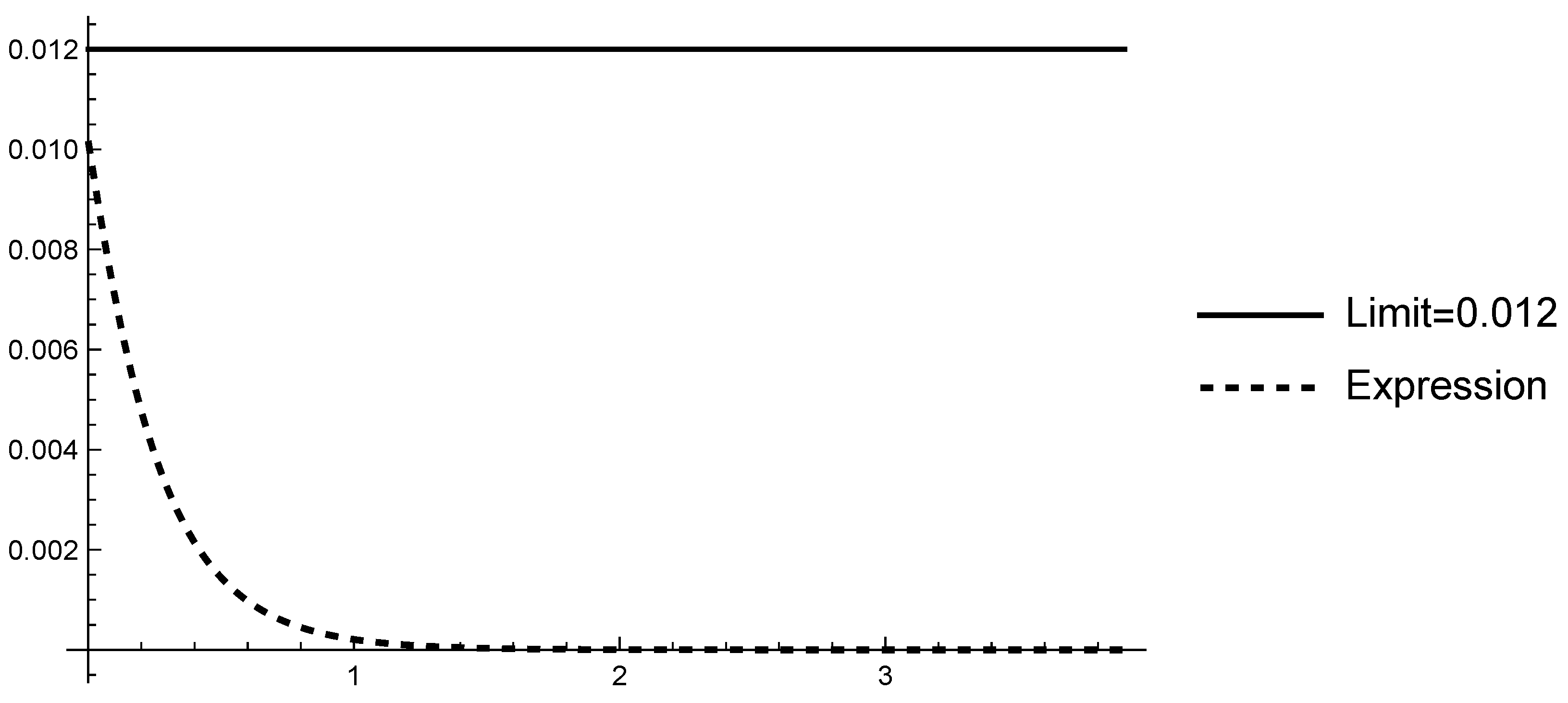
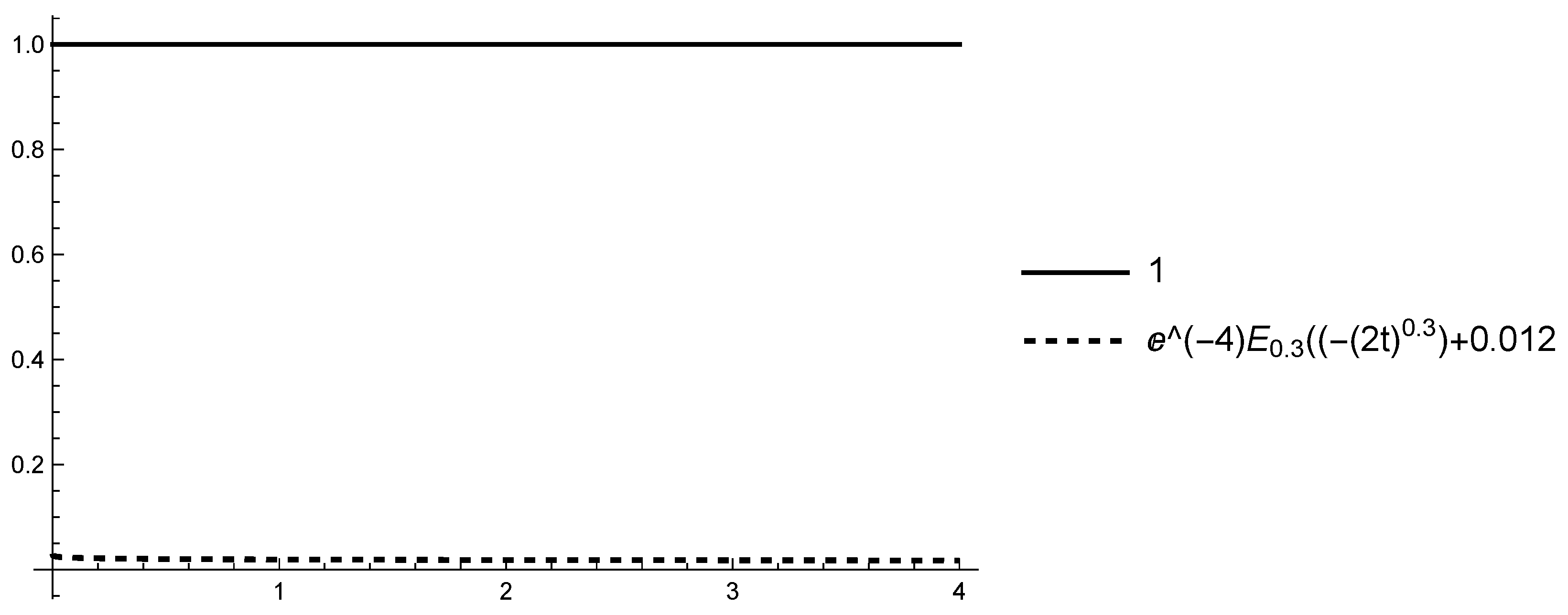
Consider the function ${\varpi }^{\left(0\right)}\left(\sigma \right)=e^{-\sigma }$. Applying the inequality $\frac{1}{0.5^{0.3}\Gamma \left(0.3\right)}{(\sigma -\tau )}^{-0.7}{e}^{\tau }{E}_{0.3,0.3}(-{\left(2(\sigma -\tau )\right)}^{0.3})\left(\frac{sin\left(e^{-\tau }\right)}{\tau +1}+e^{-\tau }\right)\le 0.012$ for $\tau \in [0,4]$ (see Figure 1) we obtain

$$\begin{array}{cc}& e^{-\sigma }\ge e^{-\sigma -4}{E}_{0.3}(-{\left(2\sigma \right)}^{0.3})\hfill \\ & +\frac{1}{0.5^{0.3}\Gamma \left(0.3\right)}{\int }_0^{\sigma }{(\sigma -\tau )}^{-0.7}{e}^{\tau -\sigma }{E}_{0.3,0.3}(-{\left(2(\sigma -\tau )\right)}^{0.3})\left(\frac{sin\left(e^{-\tau }\right)}{\tau +1}+e^{-\tau }\right)d\tau ,\hfill \\ & \sigma \in [0,4].\hfill \end{array}$$

(18)

or (see Figure 2)

$$\begin{array}{cc}\hfill 1& \ge e^{-4}{E}_{0.3}(-{\left(2\sigma \right)}^{0.3})+0.012\hfill \\ & \ge e^{-4}{E}_{0.3}(-{\left(2\sigma \right)}^{0.3})\hfill \\ & +\frac{1}{0.5^{0.3}\Gamma \left(0.3\right)}{\int }_0^{\sigma }{(\sigma -\tau )}^{-0.7}{e}^{\tau }{E}_{0.3,0.3}(-{\left(2(\sigma -\tau )\right)}^{0.3})\left(\frac{sin\left(e^{-\tau }\right)}{\tau +1}+e^{-\tau }\right)d\tau ,\hfill \\ & \sigma \in [0,4].\hfill \end{array}$$

(19)

Furthermore, ${\varpi }^{\left(0\right)}\left(0\right)-{\varpi }^{\left(0\right)}\left(4\right)=1-e^{-4}>0$ and therefore, the function ${\varpi }^{\left(0\right)}\left(\sigma \right)$ is a mild upper solution of GPDE (16).

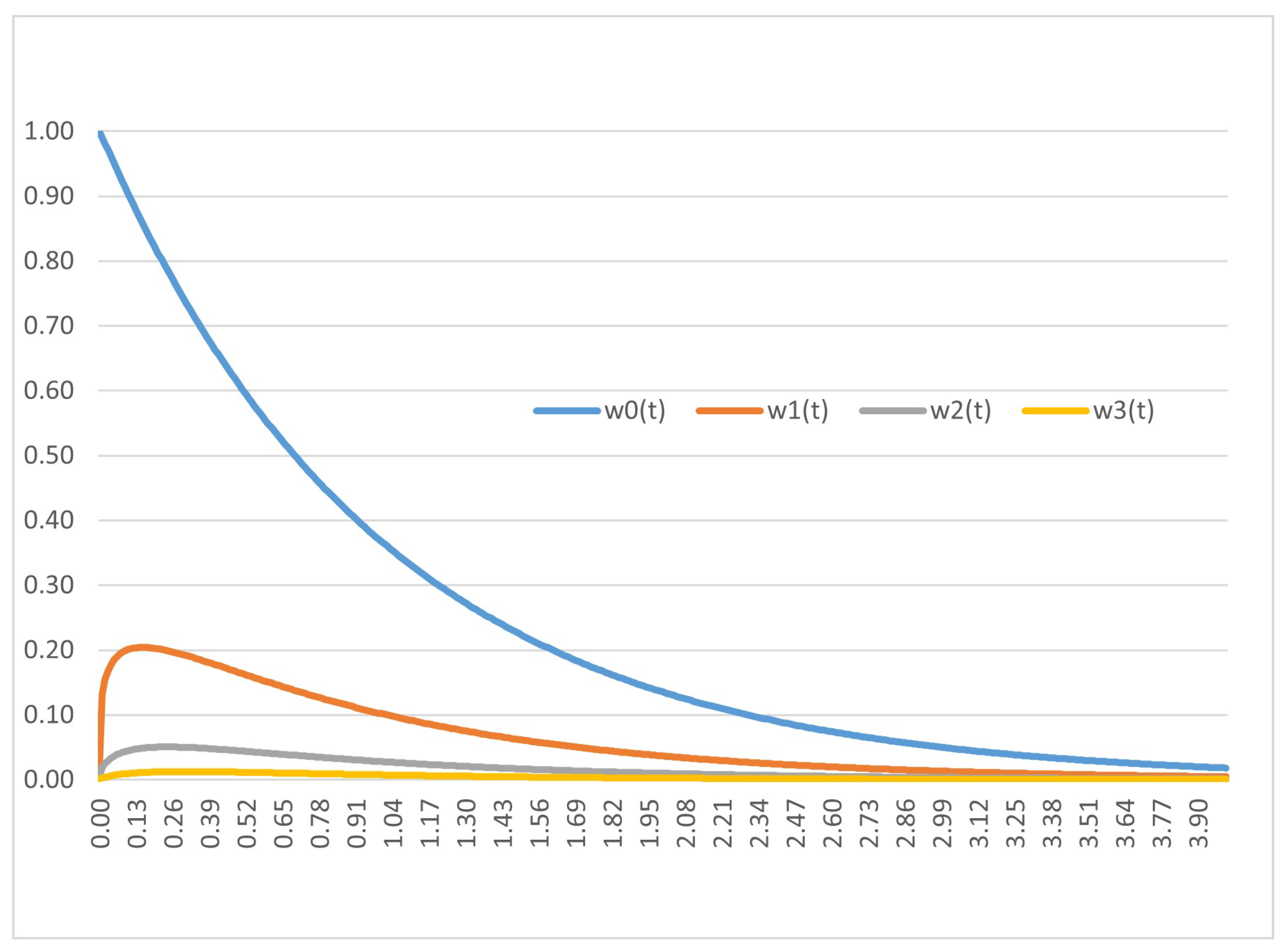
For $n\ge 0$ the approximation ${\varpi }^{(n+1)}\left(t\right)$ is obtained on $[0,4]$ by

$$\begin{array}{cc}& {\varpi }^{(n+1)}\left(\sigma \right)={\varpi }^{\left(n\right)}\left(4\right)e^{-\sigma }{E}_{0.3}(-{\left(2\sigma \right)}^{0.3})\hfill \\ & +\frac{1}{0.5^{0.3}\Gamma \left(0.3\right)}{\int }_0^{\sigma }{(\sigma -\tau )}^{-0.7}{e}^{(\tau -\sigma )}{E}_{0.3,0.3}(-{\left(2(\sigma -\tau )\right)}^{0.3})\left(\frac{sin\left({\varpi }^{\left(n\right)}\left(\tau \right)\right)}{\tau +1}+{\varpi }^{\left(n\right)}\left(\tau \right)\right)d\tau .\hfill \end{array}$$

(20)

Then the inequalities ${\varpi }^{\left(0\right)}\left(\sigma \right)=e^{-\sigma }\ge {\varpi }^{\left(1\right)}\left(\sigma \right)\ge {\varpi }^{\left(2\right)}\left(\sigma \right)\ge {\varpi }^{\left(3\right)}\left(\sigma \right)\ge {\varpi }^{\left(4\right)}\left(\sigma \right)\ge \cdots \ge 0$ hold (see

Table 1. Values of upper mild solutions ${\varpi }^{\left(i\right)}\left(\sigma \right),i=0,1,2,3,4$ for $\sigma \in [0,4]$.

$\mathit{\sigma }$	${\mathit{\varpi }}^{\left(0\right)}\left(\mathit{\sigma }\right)$	${\mathit{\varpi }}^{\left(1\right)}\left(\mathit{\sigma }\right)$	${\mathit{\varpi }}^{\left(2\right)}\left(\mathit{\sigma }\right)$	${\mathit{\varpi }}^{\left(3\right)}\left(\mathit{\sigma }\right)$	${\mathit{\varpi }}^{\left(4\right)}\left(\mathit{\sigma }\right)$
0.0	1.0000	0.0183	0.0048	0.0013	0.0003
0.1	0.9048	0.2009	0.0451	0.0099	0.0021
0.2	0.8187	0.2027	0.0505	0.0122	0.0029
0.3	0.7408	0.1928	0.0503	0.0128	0.0032
0.4	0.6703	0.1793	0.0480	0.0125	0.0032
0.5	0.6065	0.1649	0.0448	0.0119	0.0031
0.6	0.5488	0.1506	0.0413	0.0111	0.0029
0.7	0.4966	0.1371	0.0377	0.0102	0.0027
0.8	0.4493	0.1245	0.0344	0.0094	0.0025
0.9	0.4066	0.1128	0.0312	0.0085	0.0023
1.0	0.3679	0.1021	0.0282	0.0077	0.0021
1.1	0.3329	0.0923	0.0255	0.0070	0.0019
1.2	0.3012	0.0834	0.0231	0.0063	0.0017
1.3	0.2725	0.0754	0.0208	0.0057	0.0016
1.4	0.2466	0.0681	0.0188	0.0051	0.0014
1.5	0.2231	0.0615	0.0169	0.0046	0.0013
1.6	0.2019	0.0555	0.0153	0.0042	0.0011
1.7	0.1827	0.0501	0.0138	0.0038	0.0010
1.8	0.1653	0.0453	0.0124	0.0034	0.0009
1.9	0.1496	0.0409	0.0112	0.0031	0.0008
2.0	0.1353	0.0369	0.0101	0.0027	0.0007
2.1	0.1225	0.0333	0.0091	0.0025	0.0007
2.2	0.1108	0.0301	0.0082	0.0022	0.0006
2.3	0.1003	0.0272	0.0074	0.0020	0.0005
2.4	0.0907	0.0245	0.0067	0.0018	0.0005
2.5	0.0821	0.0222	0.0060	0.0016	0.0004
2.6	0.0743	0.0200	0.0054	0.0015	0.0004
2.7	0.0672	0.0181	0.0049	0.0013	0.0004
2.8	0.0608	0.0163	0.0044	0.0012	0.0003
2.9	0.0550	0.0147	0.0040	0.0011	0.0003
3.0	0.0498	0.0133	0.0036	0.0010	0.0003
3.1	0.0450	0.0120	0.0032	0.0009	0.0002
3.2	0.0408	0.0109	0.0029	0.0008	0.0002
3.3	0.0369	0.0098	0.0026	0.0007	0.0002
3.4	0.0334	0.0089	0.0024	0.0006	0.0002
3.5	0.0302	0.0080	0.0021	0.0006	0.0002
3.6	0.0273	0.0073	0.0019	0.0005	0.0001
3.7	0.0247	0.0066	0.0017	0.0005	0.0001
3.8	0.0224	0.0059	0.0016	0.0004	0.0001
3.9	0.0202	0.0054	0.0014	0.0004	0.0001
4.0	0.0183	0.0048	0.0013	0.0003	0.0001

and Figure 3). The sequence of successive approximations $\left\{w^{\left(n\right)}\left(\sigma \right)\right\}$ is a decreasing sequence and, according to Theorem 2 and Corollary 2, it is convergent and its limit is 0, i.e., the sequence is approaching the solution of GPDE (16).

Consider the function ${\varsigma }^{\left(0\right)}\left(\sigma \right)=-e^{-\sigma },\sigma \in [0,4]$. From inequality (19) it follows

$$\begin{array}{cc}& -e^{-\sigma }\le -e^{-\sigma -4}{E}_{0.3}(-{\left(2\sigma \right)}^{0.3})\hfill \\ & +\frac{1}{0.5^{0.3}\Gamma \left(0.3\right)}{\int }_0^{\sigma }{(\sigma -\tau )}^{-0.7}{e}^{\tau -\sigma }{E}_{0.3,0.3}(-{\left(2(\sigma -\tau )\right)}^{0.3})\left(\frac{sin(-e^{-\tau })}{\tau +1}-e^{-\tau }\right)d\tau ,\hfill \\ & \sigma \in [0,4],\hfill \end{array}$$

(21)

and ${\varsigma }^{\left(0\right)}\left(0\right)-{\varsigma }^{\left(0\right)}\left(4\right)=-1+e^{-4}<0$.

Therefore the function ${\varsigma }^{\left(0\right)}\left(\sigma \right)=-e^{-\sigma }$ is a mild lower solution of (16).

We construct an increasing sequence $\left\{{\varsigma }^{\left(n\right)}\left(t\right)\right\}$ which, according to Theorem 2 and Corollary 2, is approaching 0, i.e., the sequence is approaching the solution of GPDE (16).

6. Discussions about Computer Realization of the Algorithm

In the computer realization we use series for calculation Mittag-Leffler functions with an initially given error.

Before starting the calculation of the sequence of functions $w_n\left(t\right)$ defined by Equation (15), we obtain the values of the functions $E_{\gamma }(-{\left(\frac{hk}{\xi }\right)}^{\gamma })$ and $E_{\gamma ,\gamma }(-{\left(\frac{hk}{\xi }\right)}^{\gamma })$ for all $hk\in [0,4]$ where $k\ge 0$ is an integer, h is the step of the trapezoid method, $\gamma =0.3,\xi =0.5$. The results are written in two arrays $Ea\left[\right]$ and $Eaa\left[\right]$, where $Ea\left[t\right]=E_{\gamma }(-{\left(\frac{t}{\xi }\right)}^{\gamma })$ and $Eaa\left[t\right]=E_{\gamma ,\gamma }(-{\left(\frac{t}{\xi }\right)}^{\gamma })$. In computer realization we use a one-to-one relation between the real numbers $t=hk$ and the integer array indexes.

For the obtained values of $w_n\left(t\right)$ two dimensional array $w\left[\right]\left[\right]$ is used.

Initially, we could calculate $t^{1-\gamma }{e}^{-t}$ into $expr\left[t\right],t=hk\in [0,4]$.

Then, Equation (20) is reduced to:

$$\begin{array}{cc}\hfill w\left[0\right]\left[t\right]& =e^{-t},\hfill \\ \hfill w[n+1]\left[t\right]& =w\left[n\right]\left[4\right]Ea\left[t\right]+\hfill \\ \hfill & +const{\int }_0^{t}expr[t-s]Eaa[t-s]\left(\frac{sin\left(w\right[n\left]\right[s\left]\right)}{s+1}+w\left[n\right]\left[s\right]\right)ds,\hfill \end{array}$$

where $const=\frac{1}{0.5^{0.3}\Gamma \left(0.3\right)}$ and $t=hk\in [0,4]$.

We obtain the values of $w_n\left(t\right)$ for $n=0,1,2,3,4$ and for all $t=hk\in [0,4]$. We apply the trapezoid method for integral calculation.

Some of the values of the upper mild solutions, obtained by computer application of the above described algorithm, are given in Table 1, and the upper mild solutions are graphed on Figure 1. It could be seen the inequalities $w_0\left(t\right)\ge w_1\left(t\right)\ge w_2\left(t\right)\ge w_3\left(t\right)\ge 0$ hold.

7. Conclusions

The main aim is to present an algorithm for approximate obtaining of a solution of a nonlinear BVP for a scalar nonlinear differential equation with PFD on a finite interval. This algorithm is based on monotone-iterative technique combined by appropriately defined mild lower solutions and mild upper solutions. A new integral fractional operator is defined and applied to construct two sequences of successive approximations. Both sequences are monotone and they consist of lower and upper mild solutions of the studied nonlinear problem, respectively. It is proved that both sequences are convergent to the mild solution of the problem. Theoretical study is combined with a computer realization of the newly suggested algorithm and it is applied to an example to illustrate the convergence to the solution of the studied nonlinear problem.

The suggested scheme for approximate solving of the studied problem could be generalized to a system of differential equations with PFD and it could be applied to solve some particular fractional models.

References

- Das, S. Functional Fractional Calculus; Springer: Berlin/Heidelberg, Germany, 2011. [Google Scholar]
- Kilbas, A.A.; Srivastava, H.M.; Trujillo, J.J. Theory and Applications of Fractional Differential Equations; Elsevier B. V.: Amsterdam, The Netherlands, 2006. [Google Scholar]
- Abbas, M.I. Non-instantaneous impulsive fractional integro-differential equations with proportional fractional derivatives with respect to another function. Math. Meth. Appl. Sci. 2021, 44, 10432–10447. [Google Scholar] [CrossRef]
- Caputo, M.; Fabrizio, M. A new definition of fractional derivative without singular kernel. Prog. Fract. Differ. Appl. 2015, 1, 73–85. [Google Scholar]
- Atangana, A.; Baleanu, D. New fractional derivatives with non-local and non-singular kernel: Theory and application to heat transfer model. Thermal Sci. 2016, 20, 763–769. [Google Scholar] [CrossRef]
- Srivastava, H.M.; Saad, K.M. Some new models of the time-fractional gas dynamic equation. Adv. Math. Models Appl. 2018, 3, 5–17. [Google Scholar]
- Tarasov, V.E. Fractional Dynamics: Application of Fractional Calculus to Dynamics of particles, Fields and Media; Springer: Heidelberg, Germany; Higher Education Press: Beijing, China, 2010. [Google Scholar]
- Farman, M.; Akgül, A.; Ahmad, A.; Saleem, M.U.; Ahmad, M. Modeling and analysis of computer virus fractional order model. In Methods of Mathematical Modeling; Elsevier: Amsterdam, The Netherlands, 2022; pp. 137–157. [Google Scholar] [CrossRef]
- Atangana, A. Fractional Operators with Constant and Variable Order with Application to Geo-hydrology; Academic Press: New York, NY, USA, 2018. [Google Scholar] [CrossRef]
- Jarad, F.; Abdeljawad, T.; Alzabut, J. Generalized fractional derivatives generated by a class of local proportional derivatives. Eur. Phys. J. Spec. Top. 2017, 226, 3457–3471. [Google Scholar] [CrossRef]
- Jarad, F.; Abdeljawad, T. Generalized fractional derivatives and Laplace transform. Discret. Contin. Dyn. Syst. Ser. S 2020, 13, 709–722. [Google Scholar] [CrossRef]
- Shammakh, W.; Alzumi, H.Z. Existence results for nonlinear fractional boundary value problem involving generalized proportional derivative. Adv. Differ. Equations 2019, 2019, 94. [Google Scholar] [CrossRef]
- Abbas, M.I. Existence results and the Ulam Stability for fractional differential equations with hybrid proportional-Caputo derivatives. J. Nonlinear Func. Anal. 2020, 2020, 48. [Google Scholar] [CrossRef]
- Abbas, M.I. Controllability and Hyers-Ulam stability results of initial value problems for fractional differential equations via generalized proportional-Caputo fractional derivative. Miskolc Math. Notes 2021, 22, 1–12. [Google Scholar] [CrossRef]
- Boucenna, D.; Baleanu, D.; Ben Makhlouf, A.; Nagy, A. Analysis and numerical solution of the generalized proportional fractional Cauchy problem. Appl. Num. Math. 2021, 167, 173–186. [Google Scholar] [CrossRef]
- Hristova, S.; Abbas, M.I. Explicit solutions of initial value problems for fractional generalized proportional differential equations with and without impulses. Symmetry 2021, 13, 996. [Google Scholar] [CrossRef]
- Mu, J. Monotone Iterative Technique for Fractional Evolution Equations in Banach Spaces. J. Appl. Math. 2011, 2011, 767186. [Google Scholar] [CrossRef]
- Somjaiwang, D.; Ngiamsunthorn, P.S. Existence and Monotone Iterative Approximation of Solutions for Neutral Differential Equations with Generalized Fractional Derivatives. J. Math. 2022, 2022, 1239701. [Google Scholar] [CrossRef]
- Bai, Z.; Zhang, S.; Sun, S.; Yin, C. Monotone iterative method for fractional differential equations. Electr. J. Diff. Equations 2016, 2016, 1–8. [Google Scholar]
- Wang, G. Monotone iterative technique for boundary value problems of a nonlinear fractional differential equation with deviating arguments. J. Comput. Appl. Math. 2012, 236, 2425–2430. [Google Scholar] [CrossRef]
- Cui, Y.; Sun, Q.; Su, X. Monotone iterative technique for nonlinear boundary value problems of fractional order p∈(2,3]. Adv. Differ. Equations 2017, 2017, 248. [Google Scholar] [CrossRef]
- Chen, P.; Kong, Y. Monotone Iterative Technique for Periodic Boundary Value Problem of Fractional Differential Equation in Banach Spaces. Int. J. Nonlinear Sci. Numer. Simul. 2019, 20, 595–599. [Google Scholar] [CrossRef]
- Song, S.; Li, H.; Zou, Y. Monotone Iterative Method for Fractional Differential Equations with Integral Boundary Conditions. J. Fuct. Space 2020, 2020, 7319098. [Google Scholar] [CrossRef]
- Baitiche, Z.; Derbazi, C.; Alzabut, J.; Samei, M.E.; Kaabar, M.K.A.; Siri, Z. Monotone Iterative Method for ψ-Caputo Fractional Differential Equation with Nonlinear Boundary Conditions. Fractal Fract. 2021, 5, 81. [Google Scholar] [CrossRef]
- Podlubny, I. Fractional Differential Equations; Academic Press: San Diego, CA, USA, 1999. [Google Scholar]
- Agarwal, R.; Hristova, S.; O’regan, D. Stability of Generalized Proportional Caputo Fractional Differential Equations by Lyapunov Functions. Fractal Fract. 2022, 6, 34. [Google Scholar] [CrossRef]
- Zhou, Y.; Jiao, F. Existence of mild solutions for fractional neutral evolution equations. Comput. Math. Appl. 2010, 59, 1063–1077. [Google Scholar] [CrossRef]
- Sousa, J.; Abdeljawad, T.; Oliveira, D.S. SMild and classical solutions for fractional evolution differential equation. Palestine J. Math. 2022, 11, 229–242. [Google Scholar]
- Ardjouni, A.; Guerfi, A. On the existence of mild solutions for totally nonlinear Caputo-Hadamard fractional differential equations. Results Nonlin. Anal. 2022, 5, 161–168. [Google Scholar] [CrossRef]