Abstract
In control research and design it is frequently necessary to explore, evaluate, tune and compare many control strategies. These activities are assisted by software tools of increasing complexity; however, even with the existing high performance tools these activities are very time consuming due to they imply hundred if not thousand of simulations. If the process of doing such simulations is not automated it can be a very time consuming task. There has been proposed evolutionary algorithms (EA) that in the search for an optimal control automatically generate many control structures. However, the space of possible controllers for any dynamical system is huge. Hence it is mandatory to restrict the search space. The best way to restrict the controller search space is to let the designer influence the search direction. In this paper we propose a software tool for control research that has as its main part an EA that produce only controllers having a pre-specified morphology. By specifying a controller morphology the designer can influence the search direction without losing the exploration capability of evolutionary algorithms. The EA is endowed with a cost function tailored for fast evaluation of closed-loop controller performance. The use of the tool is illustrated by searching an sliding mode and similar controllers for an unstable linear and two nonlinear systems.
1. Introduction
In control theory research, is common to rely on software tools for explore, evaluate, an tune control strategies. These tasks are time consuming, even with software tools of increasing performance and complexity. If in addition, researchers want to evaluate different control alternatives and variations they have to perform hundreds, even thousand o simulations; consequently they need to dedicate long periods of time on simulation tasks. This paper is aimed to reduce such time by providing a software tool to automate the task of controller exploration, evaluation and tuning.
Recently, evolutionary algorithms (EA) for automatic controller generation has been proposed [1,2,3,4,5,6,7,8,9,10,11,12,13,14,15,16]. These algorithms begin by creating a set of elements, called the initial generation. From the initial generation, successive generations are derived by creating a new generation from the previous one. In control applications of EA, each element of every generation is a controller, that is, a mathematical expression of system state. Elements of initial generation is created by a random combination of parameters and functions of the error and state variables [12,17,18,19]. Roughly speaking, to derive a next generation from the current one, the following steps are carry-out: (a) performance of each element is evaluated using a cost function; (b) fitness is assigned to each element according to its performance; (c) some elements of the current generation are selected based on its fitness; (d) selected elements undergo a process called genetic operations to produce other elements. The process of selecting elements and apply a genetic operation is repeated till a complete new generation is created.
EA have been applied to a great variety of control engineering problems, from tuning of classic controllers, to generation of free-form controllers. Just to name a few, in [7,20,21] genetic algorithms to tune PID controllers for an electro-hydraulic valve; continuous stirred tank reactor; and 3DOF robot system are proposed, respectively. In these works, each element of a generation codes a PID controller; the algorithm ends when a good enough controller is obtained. Authors of [20] compare traditional PID tuning with several metaheuristics algorithms; they conclude that development of metaheuristic algorithms for effective optimization and controller tuning is still remains an active research area for academicians and industrial practitioners. In [7,20,21], structure of controllers do not change along the algorithm execution, hence the algorithm is aimed to search the best combination of controller parameters. On the other hand, EA proposed in [8,19,22] can create and evaluate a great number of controllers; however the possible number of controllers for any dynamical system is huge. The search space can be reduced by restricting the kind and number of functions allowed in the creation of controller. However, it would be convenient that in addition to this form of restriction, the researcher could specify the kind of controllers to search. Restricting the kind of controllers the algorithm is able to produce is advantageous because when a researchers deal with a problem, usually they have previous knowledge about the system; such knowledge can come from heuristics, mathematical analysis, experience, close examination, etc. In any case, a researcher generally have an idea of advisable controller techniques to solve the problem at hand. Furthermore is would be advantageous to be able to test some variations on the controller structure.
It would be very useful to have a tool able to search controllers with some variations around a pre-specified controller structure. In this manner, the knowledge of the engineer would be present through the pre-defined structure but at the same time, variations around it would be allowed. In this paper such a tool is provided. The tool has as its main part an EA that only generates controllers of a pre-specified morphology. The EA here proposed includes a cost function for fast evaluation of closed loop performance. The proposed cost function is tailored for automatic simulation and fast evaluation of controlled systems; in addition to the standard error norm, it includes a term to measure the steady state error and another term to compare unstable controllers. These last two features increase the algorithm convergence without adding too much complexity. Such cost function has a major influence on the controllers generated since the algorithm rules to create new elements intend to create controllers that minimize the cost function similarly to the formal optimization methods [23,24,25]. However, EA do no require the computation of derivatives which formal methods one way or another are required to do.
Summing up, in this work, a software tool to save a considerable amount of time to control theory researchers by reducing the time they spent on doing simulations. Such tool enable them to (a) introduce the system that they are working on and (b) introduce their assumption of what control strategy could be suitable for the system. The system can be any single-input single-output (SISO) nonlinear affine control system. The control strategy is specified by establishing a morphology that the controller must satisfy. Controllers morphology can be chosen to be slightly general; thus, the search space is still wide, but the search trajectory is influenced by the designer knowledge. A morphology to test several sliding mode control (SMC) variations is used in present work as an example; however, by examining how the algorithm only produce sliding mode controllers and the available source code (https://github.com/control-lab-org/HTSMC (accessed on 3 July 2023)) [26], interested readers can implement other morphologies on their own. SMC is chosen because it is suitable for linear and nonlinear systems; Sliding mode controllers are known to be robust under parameter variations, with a fast response, good external disturbance rejection and generally, easy to implement.
The tool here developed has as its main part an EA that only generates controller of a prespecified morphology. The EA is equipped with a cost function specifically designed for automatic fast evaluation of closed-loop controller performance. However, it is important to point out that the tool developed also allow (a) to easily describe any SISO nonlinear affine control system; (b) to simulate such sytem with any controller; (c) to save every generated controller in a run and its fitness; (d) to save the five best controllers at each generation and it fitness; (e) to show the evolution of the cost function along generations; (f) to automatically plot the performance of the best five controllers at each generation; (g) to use the last generation of a run as the initial generation of another. These features are not described in depth due to the interested reader can examine the source code included in suplemental material of present work. Furthermore some of these characteristics has been (similarly) implemented in [19]. It must be pointed out, however, that in this work it is done in simple manner and only free software is employed.
The rest of the paper is organized as follows: In Section 2 the kind of control problems addressed in this paper is precised and an overview of the main part of the developed tool, that is the EA employed is presented. From then on, the algorithm is described more precisely. Section 3 precise what it is advantageous that the controllers generated by the algorithm have a pre-specified morphology. In Section 4, the creation of initial generation is described. Section 5, explain how the elements are evaluated. In Section 6 it is described how the next generation is constructed. In Section 7, some details of when the algorithm ends are given. In Section 8, some results obtained using the tool are presented. Finally in the last Section some conclusions are given.
2. Control Problems Addressed and General Description of the Tool Developed
The kind of systems that the developed tool address is
where ; ; ; ; and r is a constant. The control objective is to build u such that .
The general system described by Expression (1) includes all single input, single output dynamical systems that is in any of the following categories:
- Can be described by a transfer function
- Linear systems that can be described by
- Affine nonlinear systems that is nonlinear system where the control appears in linear form.
Such systems includes many chemical process, electrical systems, electronics power converters, electro-mechanical systems systems, etc.
As was mentioned on the previous Section, the proposed tool are composed of several parts among which the main if an evolutionary algorithm that only produce controllers with a pre-specified morphology. The here developed tool has other parts including: the software to automatically simulate any SISO nonlinear affine control system, controlled by any controller. These parts of the proposed tool are not described in depth due to the interested reader can examine the source code of the tool included in suplemental material of this work and in (https://github.com/control-lab-org/HTSMC (accessed on 3 July 2023)). Some features of the developed tool are similar to what has been done in [19]; however, is worth noting that in this paper only free sofware is employed. In the rest of this Section an overview of the proposed EA is presented.
Evolutionary algorithms start with the creation of a set of non-optimal potential solutions (the initial generation) and then creating a new set of solutions (a next generation) from the existing one. In control applications, creating the initial generation means to build a set of controllers. The elements of the next generation are derived from the existing generation. By the creation of successive generations, initial controller (elements of the first generation) are modified; terms are added, removed or adjusted through a selection mechanisms and so called genetic operations (GOs). Hopefully, each new generation is somewhat better than the previous one. The process of creating the next generation stop when a near optimal solution is found.
In Figure 1, it is depicted the flow diagram of the algorithm; symbols of the figure mean:
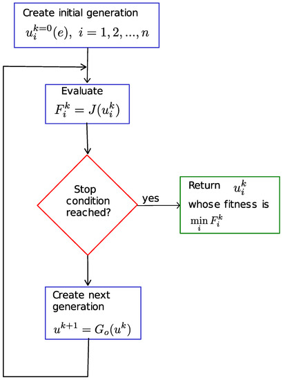
Figure 1.
Flow diagram of the evolutionary algorithm employed.
- is the k-th generation.
- is the i-th element of the k-th generation.
- is the fitness of .
- is the cost function evaluated at .
- represent the set of genetic operations that take a generation and provides a new one.
The algorithm proceed as follows:
- Step 1: An initial set of controllers is created at random. This set of controllers is the initial generation .
- Step 2: Each element of a generation is evaluated: . Based on how well an element solves the problem a fitness is assigned to it.
- Step 3: Examine the stop condition. Such condition should check in someway if a near optimal control has been found.
- Step 4: If stop condition has not been reached, a next generation is created: . To this end, selection mechanisms and genetic operations is employed, and the process is repeated from step 2.
Figure 1 and previous steps is a general description of the algorithm. However what distinguishes the here proposed algorithm are the process of creation of initial generations, evaluation of controllers and creation of next generation. These processes will be described in Section 4, Section 5 and Section 6 respectively. In the next Section advantages of specifying a morphology to restrict the controller search space is precised.
3. Advantages of Specifying a Morphology in Controllers Creation
In EA for control applications each element of every generation is a controller. To create a controller a tree structure is commonly used [19]. In present work the notation of Scheme programming language [27] is used to represent tree structures in textual form as is shown in Figure 2. Controllers are specified by nodes and leaves; nodes are formed by math operators and leaves are its operands. Operators can be unary or binary; operands can be symbols or numbers; usually symbols denote state variables and numbers are controller parameters. To create a random controller a set of nodes and a set of leaves are needed. These sets can be represented as:
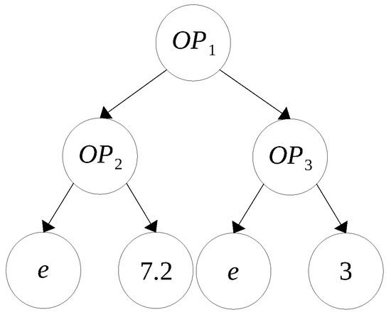
Figure 2.
Graphical tree representation of the scheme expression ( ( 7.2 e) ( 3 e)).
At the same time
- is a set of unary operators.
- is a set of binary operators.
- is a set of symbols.
- is an interval, that is a set of parameter values.
To create a simple controller an element of set is picked a random, the result hast to be the set or the set. If is chosen then an unary operator is picked at random; on the contrary, if is chosen then an binary operator is picked at random. Depending on what type of operator results, one or two leaf is needed. In any case, a leaf is created picking one element of the set , that yields the set or the set ; if the result is the set of then a symbol is piked at random, on the contrary, a number within the interval is picked at random. The following six general cases can result from this process
Where , , and . Note that depending of the size of sets of , and many controllers can be generated from this simple process. Moreover, any leaf can be substituted by a tree to obtain a tree of depth 2 like in Figure 2. Similarly a tree of depth 3, 4 an so on, can be obtained. The number of possible controller can be huge even for small size of sets , , and .
In EA proposed till now, the set of controllers that can be created, that is the search space, is limited only by the operators allowed to be used and the maximum depth of the tree [19]. When the operators allowed and the maximum depth of the controller tree are the only restrictions in the evolution of elements there are two inconvenient
- The search space size causes algorithm converge very slowly or not converge at all.
- It is not possible to take advantage of the apriori knowledge that the control engineer may have about the system.
In present work restrictions in the kind of controllers the algorithm is able to generate are imposed. More precisely, controllers created must have a given morphology. If controllers that the algorithm generates always has the same morphology, the researcher can influence the evolution process; hence, researcher could decide to use state feedback controllers, discontinuous controllers, state feedback linearization controllers, PID controllers, etc. For example, if an engineer knows that a system can be controlled by a PI/PID control, then she could establish the morphology
where is the controller system state variable; , and are constants that determine the controller dynamics and u is the controller output. Since all PI/PID controllers can be expressed using (3), by restricting the algorithm to only produce controllers that have the morphology given by (3), the researcher will in fact be searching the optimal PI/PID controller for the system. If controllers are restricted to have a given morphology an user could apply EA to situations like (a) exploration of the effectiveness of a given control structure or a set of control structures; (b) parameter tuning, etc.
4. Creation of Initial Generation
In this work, a morphology based on the typical expression of sliding mode controllers is employed as an example. However, other morphology could be used as well. Sliding mode control is used because it is known to be robust, can achieve zero steady state error without an integrator and has finite time response.
It is well known [28,29] that a typical sliding mode controller for system (1) has the form.
where is a constant which will from now on, known as switching gain; the function of the state defines the surface known as the switching or sliding surface and is also a function of the state. With the proposed algorithm, it is easy to explore other structures, for example it can be included controllers with the form
where all the symbols mean the same than in (4); in addition the operator is a binary operator chosen at random. Note that morphology (5) is more general than (4).
Discontinuous right hand systems like the system (1), (5) are slowly to simulate. Due to EA needs a simulation to evaluate each element of a generation, the number of simulations could be big, hence the algorithm execution time could be large in excess. Therefore in some situations can be convenient to approximate the function in (5) by a tanh function; So, Expression (5) can be approximated by
Having the general form of a controller given by (6), the element of the generation k can be expresed as
Summing up, the proposed algorithm can be used to explore, test and evaluate controllers of the Forms (4)–(6) and particular cases, for example the case of in all the previous forms. Note that there are many nonlinear controllers of the form (6). From the ideas of present and next Sections other morphologies can be implemented.
A controller with morphology given by (6) can be represented by the tree depicted in Figure 3. It is important to point out that every controller the algorithm generates must have this morphology. To create an element (controller) with the purposed morphology is necessary to:
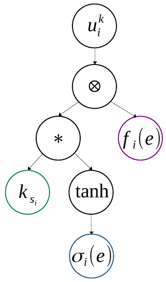
Figure 3.
Tree representation of proposed morphology where: and ∗ is the scalar multiplication sign.
- Choice the value
- Choice the ⊗ operator
- Build the function
- Build the function
The selection of is straightforward; is just to generate a random number within the interval . Selection of ⊗ is also direct; it is chosen at random from a list of symbols. To build function and the process of creating a simple controller, described above is perform. Note, that this is a recursive process. Such process is not difficult to program in high level programming languages such as Python or Lisp-like languages. The code for the algorithm an indeed for all parts of the tool developed in this paper can be consulted in https://github.com/control-lab-org/HTSMC (accessed on 3 July 2023).
Suppose that and the depth of trees of and are . Then some resulting examples from this process are
5. Evaluation of Elements of a Generation
5.1. The Environment
As has been observed, elements of every generation are controllers. To evaluate each element means to determine how well each controller performs. To this end a closed-loop control system (CLCS) must be constructed and simulated for each element. To construct a CLCS for each element the following components must be taken into consideration
- A reference signal.
- A controller (the element itself).
- The dynamical system.
- External perturbations.
- Simulation parameters.
These components together form ‘the place’ where an element will be tested. In order to determine how suitable it is to do its job. Such ‘place’ is usually called the environment (see Figure 4).
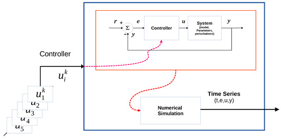
Figure 4.
Block diagram of the environment created for evaluation process.
The evaluation process must provide a score of how much good an element is. This score is called the element fitness. A higher fitness means a better element. In control problems, a cost function is employed to rate a controller performance. A good controller results in an small cost. The smaller the cost, better results the controller has. A smaller cost is equivalent to a higher fitness and vice-versa.
To compute its cost, every element is tested under the same environment, that is, a numerical simulation of the CLCS for each element is performed. From the simulation a collection of time series (TS) are obtained. The output y, the input u, the reference r, the error e and the time t values are collected. Using these signals the cost/fitness of each element is calculated as it is described below.
For each element (controller) of a generation the closed-loop of the controller and the system is build and simulated. In this subsection, it is described how this process is done.
The plant is described by state equations in the usual form of Nonlinear Systems (1). All the information necessary to simulate the system is encapsulated into an object that collect all the information about the dynamic system, which was called . More precisely, this object has the following data:
- System name
- Symbols used for state variables
- State equations
- Output expression
- Symbol used for input
- Symbols used for parameters
- Parameter values
For example, the Scheme language code shown in Figure 5 describes the system given by
with , , , , and initial conditions and .
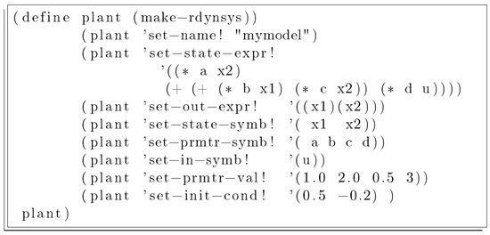
Figure 5.
Example of the definition of a system to be evaluated.
Closed-loop simulations are performed using the XppAut [30] software. XppAut is used because it is fast, and represent a dynamical system in textual form very similar to the standard notation of state space representation and it is free. Having the plant described by means of a object, it is not difficult to translate the plant state equations into XppAut; the interesting part is the translation of the prefix form used in plant description to the infix form used in XppAut. However this is a common task that has been programmed before [27]. Translation of the controller expression to XppAut is along the same as the translation of plant description.
Some disturbance signals can be introduced into the simulation of each controller. This simulates the confrontation to adverse conditions that the element suffers during its evolution into the environment.
Having the closed-loop expressions of the controller-plant in XppAut the simulation is performed and the time-series corresponding to the controller being evaluated is generated. From this time-series the cost, and hence the fitness of the controller is calculated as it is described in Section 5.2.
The evolutionary algorithm is independent of the simulation software; the created object contains all the information about the system and a layer of code between the system-controller description and simulation software was created. In present work, XppAut is used as simulation motor. The library translates the description system into a readable XppAut simulation file. However, if the simulation software changes, just a new library that translate the system-controller to the new software syntax would be necessary.
5.2. The Cost Function
A cost function tailored for automatic fast evaluation of a closed-loop controller performance is a main part of the proposed algorithm. Typically in optimal control algorithms, including EA, the norm of the error is used as cost function [23,31,32,33]. In this work, a linear combination of several functions is proposed similar to [34]. The objective of the proposed cost function is to measure some factors of the error signal that are important in control systems. Generally it is desirable that the cost function increase its value in any of following situations:
- The output does not track the reference.
- The output diverges from the reference.
- The steady state error is large.
Below, it is proposed a cost function that quantify these situations.
5.2.1. Measuring the Reference Tracking
The reference tracking error is defined as the distance between output and its reference signals. The most common distance definition used between these two signals is the norm. It is also one of the most common cost-function used to compare the elements. In view of it is well-known that it generalizes the Euclidean distance between the output and its reference. As a result, is defined as
5.2.2. Measuring How Fast the Output Explode in Unstable Systems
It is common that the proposed EA generates many unstable controllers particularly in the first generations. Instead of discard these controllers is very useful to compare two of them, because the “less unstable” could be evolve to a stable one. In present work, XppAut software [30,35] is used to compute the numerical values. In order to evaluate when a control law causes an unstable response a characteristic of XppAut is used. XppAut has a pre-specified bound, that is the maximum value a variable can reach in magnitude. The program triggers an overflow event and stop the computation. This event truncates the resulting time-series, that is, a shorter time-series is obtained than the will be expected if the simulation had not been stopped. This can be used to measure the divergence speed, in other words, how fast the system ‘explode’, using the expression
where is the initial time; is the total simulation time, that is the time that simulation would take if the system does not explode; is the time at which the system explode, that is the time where any state trespass the acceptable bound.
From (13) it can be observed that if simulation is completed then . On the other hand if simulation is truncated by out-of-bound event, that is then . The smaller , closer to 1 is . Hence is a measure of how unstable a system is.
In Figure 6 there are compared two output signal caused by two different control-laws, and , for the same system. In the figure, ; ; and are error functions obtained with and respectively; is the bound for e, that is, the simulation stops when ; signals and explode at and respectively. In the figure and . According to (13) this result on and , which agree with the fact that explode sooner than . Note that, according to (13), , so it is convenient to scale its value, in order to make it more significant.
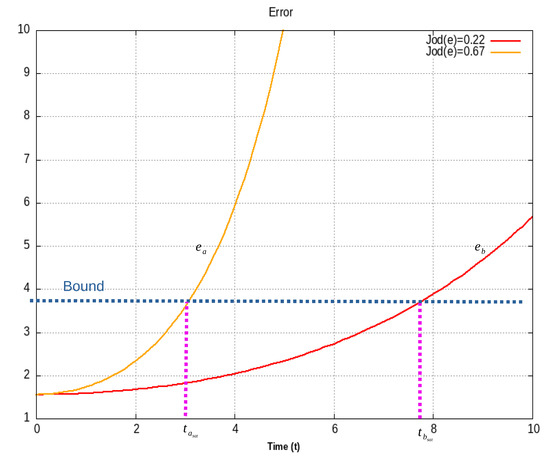
Figure 6.
Measuring closed-loop system instability.
5.2.3. Measuring the Steady State Error
Most systems have transient effects at the start of the response. For stable systems such effects vanish with the time. On the contrary, stationary behavior does not disappear with the time. A cost function that somewhat measure the steady state error must ponder lightly the error at the start of response and weigh heavily the error at the end of the response. Here, it is proposed
5.2.4. Total Cost Function
Having the costs functions described above, it is proposed to use a weighted combination of all of them, that is, the total cost function if given by
where constants and , are used to influence the search direction. A higher weight in one factor, means that the algorithm will search controllers that reduce such factor. Substituting (12)–(14) in (16) yields
6. Creation of Next Generation
At the stage of creating the next generation it is necessary to make sure that genetic operations keeps the morphology established in the initial generation. Below it is explained how to restrict the evolution process to keep the morphology given by (6). For other morphologies the genetic operations must be changed accordingly. First the general ideas for the creation of the next generation in EA are shown and summed up in the Figure 7.
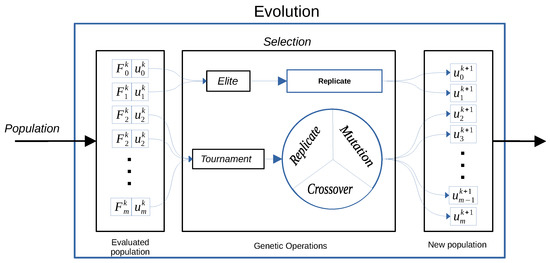
Figure 7.
Evolution Process.
6.1. General Process for Creation of Elements of the Next Generation
After the elements of a generation has been evaluated, their fitness is known. Using the fitness of each element the natural selection ca be somewhat imitated to create the next generation from the current one. Procedures that define the changes that the element undergo are known as genetic operations (GO). Several of these procedures has been proposed along time. Among the most common are:
- Replication: This function does not modify the element at all. This operation propagates the element without taking its performance into account.
- Mutation: This operation modifies only a specific part of and element.
- Crossover: Create a new element combining two current element called parents.
The selection of elements that are fed to genetic operations to create elements of the next generation can not be completely deterministic; some random process is necessary to imitate the natural selection and adaptation. Different methods to carry out such random process has been proposed; from purely random selection, roulette method or tournament method to name a few. In the results reported below, replication of the elite and tournament was selected because elements with better performance have more opportunity to evolve.
- Replication of the elite
Replication of the elite means to select a number of elements with the highest fitness. Such elements are called the elite. The elite is selected to be part of the next generation without change in its structure or parameters. This makes sure the best elements are part of the next generation.
- The tournament
Once the elite is propagated to the next generation, the tournament process, described below, is run iteratively to create element after element till the next generation is complete. The tournament consist in the following steps:
- Exclude the elite and select a subset of elements randomly.
- The best element of this subset is fed to a genetic operation (replication, mutation or crossover).
- If the chosen genetic operation were crossover, a second element is needed to be fed to the genetic operation; such second element is taken at random from the subset of selected elements by the tournament.
- The genetic operation result in a new element which is part of the next generation.
6.2. Keeping the Morphology of Elements through Generations
The only step where elements could change of morphology is through genetic operations (GOs). Therefore, to keep the morphology of elements through generations, it is necessary to restrict the changes, such that the new elements also have the same morphology. To always produce elements with the morphology given by (6) GOs used in present work (mutation, crossover and replication) are only between the same part of the general Expression (6). That is, mutations only modify the switching gain or the sliding surface or the function . In the same way, crossover, is restricted to combine two switching gains , or two sliding surfaces , or two functions , .
6.2.1. Mutation Operations
Mutation of switching gain to create another, can be written as
where does not mean a strict mathematical function but a procedure that take a constant and generate another constant. Procedure can be any of two possibilities:
where r is random value.
Mutation of sliding surface and general function to create another, can be expressed as
where is a procedure that takes a tree and produce another; the mutation procedures used in this work are the same described in detail in [19].
6.2.2. Proposed Crossover Operations
The crossover operation of two gains can be written as:
where is a procedure that takes two switching gain values , and generates a new one. Procedure can be any of three possibilities:
Crossover of two sliding surfaces , can be written as
In the same way, crossover of two general functions , can be written as
where is a procedure that take two trees and produce another tree; such procedure can be any of those depicted in Figure 8 and Figure 9. The precise way of how mutation and crossover are done is better expressed by code. Source code of this work can be consulted in https://github.com/control-lab-org/HTSMC (accessed on 3 July 2023) [26].
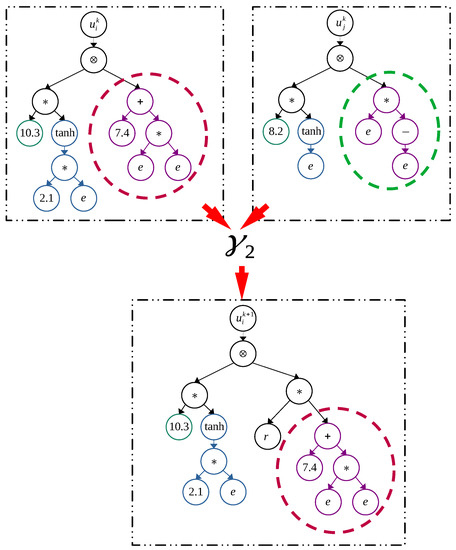
Figure 8.
Crossover: Branch scale. Where: and ∗ is the scalar multiplication sign.
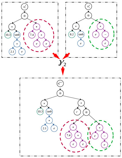
Figure 9.
Crossover: New branch. Where: and ∗ is the scalar multiplication sign.
Having specified how mutation and crossover operations are performed, creation of a new controller is as follows: with reference to Figure 10, pick at random only one branch A or B. If A branch is selected, pick at random the sliding surface or the switching gain . If the B branch is selected then it corresponds to . Once , or has been chosen, create a new controller by performing the operation that the tournament mandates, that is perform a mutation or crossover operation as has been previously described.
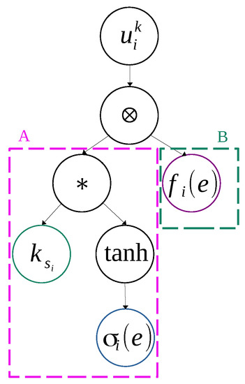
Figure 10.
Tree codification of control law. Where: , ∗ is the scalar multiplication sign, A is the SMC branch and B the branch corresponding to free function .
7. Stop Condition and Algorithm Parameters
For the sake of the algorithm description be self-contained, in this Section it is described when the algorithm stop and several parameters that can be set to tune the algorithm behavior.
The most common method to stop the algorithm is to specify a maximum number of generations. In addition, if the best average fitness of a generation, does not improve within (specified) number of generations then the algorithm is stopped and the best element so far is returned as the near optimal control.
There are some general parameters that can be modified in order to conduct the search process. All of them are constant during the algorithm execution. Some of the most important parameters are:
- Algorithm parameters
- –
- Generation size: It indicates the number of elements of each generation, these are the search agents in the search field of potential solutions.
- –
- Range of the constants: It establishes the range of the random numeric constants.
- –
- Depth: It determines the minimum and maximum number of sub-trees that a controller can have.
- –
- Elite-Size: The number of the best elements that are copied directly to the next generation.
- –
- Genetic Operation probability: The relative probability of an element to be operated by replication, mutation or crossover.
- Stop condition parameters
- –
- Maximum number of generations
- –
- Maximum number of generations without average fitness improvement
- Simulation parameters
- –
- Simulation time
- –
- Max integration step size
- –
- Integration method
8. Results
To show the flexibility and convenience of tool developed in present work, it is applied to three test experiments: An unstable linear system, the simple pendulum and the boost power converter.
8.1. Application to an Unstable Linear System
Consider the unstable system given by
where and . The transfer function (23) can be described in space state model as
Using the system parameters and with the EA parameters shown in Table 1, the best controller obtained was

Table 1.
Parameters used in the algorithm.
In Figure 11 the response of the unstable system (24) controlled by (25) is shown. The reference is given by
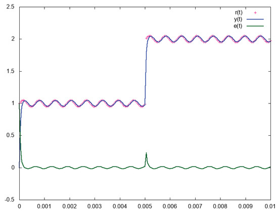
Note that controller (25) was obtained after 3000 simulations performed automatically. Furthermore, the algorithm does not know anything about the system; however, the knowledge of the researcher is embodied in the controller morphology.
Similar results were obtained every time the tool was run for this system. Testing for different a values returned similar results.
8.2. Application to the Non-Linear Simple Pendulum
The motion of a simple pendulum can be described by
where is the pendulum angle. Model (27) is a simple non-linear second-order system with multiple equilibrium points useful as benchmark. A common control goal is to find a direct input-output static control that tracks a reference and reject perturbations when the reference is near the unstable equilibrium point.
System (27) can be expressed in state space model by
Using the pendulum parameters , , , and the algorithm parameters shown in Table 2, the best controller obtained with the developed tool is given by
where
Table 2.
Parameters used in the algorithm.
Figure 12 and Figure 13 show two responses of the system (28) controlled by (29) and (30). Figure 12 shows the results when the reference suddenly changes. Figure 13 shows the output when the system is perturbed by an impulse on the output. It can be observed from these figures that the output signal tracks a changing reference and reject external perturbations. Similar results were obtained every time the tool was run for this system. It is interesting to note that to obtain this result, simulations were automatically performed.
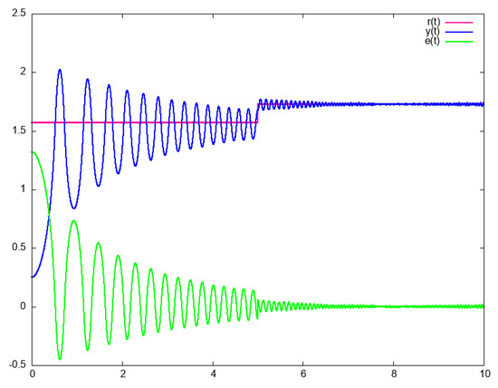
Figure 12.
Response of system (28) with a reference change at t = s.
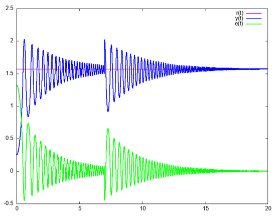
Figure 13.
Response of system (28) with perturbation in the output at t = s.
8.3. Application to the Boost Converter
To show the flexibility of the developed tool to deal with different kind of systems, it was applied to a third system very different to the previous two: the boost converter [36]. The boost converter is a nonlinear, non minimum phase system, with bounded control described by
where is the inductor current, is the capacitor voltage, R is the circuit load, C is the capacitor value, L is the inductor value and is the input voltage. The system output is the load voltage, that is the same as the capacitor voltage. It is well known that this system is difficult to control due to it is nonlinear, non-minimum phase with bounded control. Such characteristics made a typical benchmark to test nonlinear control strategies.
The control objective is . The tool here developed, was applied to system (31) using , L = 500 uH, C = 47 uF and = 5 V. A sudden changing reference was used:
where nominal value is = 24 V and is the Heaviside step function. The time related values of all simulations were = 10 mS, = 3.33 mS, = 6.66 mS. The algorithm parameters are shown in Table 3. With previous conditions and values the best obtained controller in a run of the tool, results
Note that controller (33) was obtained after 25,000 simulations automatically performed. The closed-loop performance of system (31) with controller (33) is shown in Figure 14.
Table 3.
Parameters used in the algorithm.
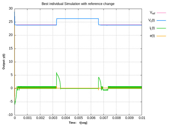
Figure 14.
Response given by automatic generated controller (33).
9. Conclusions
In this work a tool to automate simulations has been developed. Due to control researchers usually spend hours and some time days performing simulations, the tool here presented can help them save much time. The tool, has several parts among which the main is an evolutionary algorithm that only produce controllers with pre-specified morphology. An important component of the evolutionary algorithm here proposed is the cost function employed. Such cost function, efficiently compare the steady state error and instability of two controllers.
The development of the tool here presented was motivated by the idea that previous proposed EA could be used to generate a great number of controllers; however in such algorithms the user was not able to include her previous knowledge on the system. With the tool here developed a researcher can know use EA for exploration of controller structures and at the same time take advantage of her previous knowledge on control theory and particularly on the problem at hand.
To show the power and flexibility of the tool here developed was applied to three very different systems. In all of them, after of several hundred of simulations automatically performed, a suitable controller was found.
Many experiments can be derived from this work, for example the common questions of: What if I add an integral/derivative term? What if I add/eliminate a discontinuous term? What if I approximated the sign with tanh? and many other similar question could be answered.
Another way to see the tool here developed is as a tool to make a great number of simulations guided by our previous experience and knowledge on control theory and the problem at hand. Depending on the system complexity thousand of simulation can be performed in a few minutes. Since thousands of simulations can be automatically performed, researchers can address, explore and compare several control strategies for a single system.
Is advisable to extend the tool to be able to deal with multi-input multi-output systems.
Author Contributions
Conceptualization, F.-D.H., D.C., M.A.R.-S. and L.A.V.-V.; methodology, F.-D.H. and D.C.; software, F.-D.H.; validation, D.C., M.A.R.-S. and L.A.V.-V.; formal analysis, D.C.; investigation, D.C., M.A.R.-S. and L.A.V.-V.; resources, M.A.R.-S. and L.A.V.-V.; data curation, D.C.; writing—original draft preparation, F.-D.H.; writing—review and editing, F.-D.H., D.C. and M.A.R.-S.; visualization, F.-D.H. and D.C.; supervision, D.C. and L.A.V.-V.; project administration, L.A.V.-V.; funding acquisition, L.A.V.-V. All authors have read and agreed to the published version of the manuscript.
Funding
This research was funded by Instituto Politécnico Nacional of Mexico and CONAHCYT of Mexico.
Data Availability Statement
The research data and source code is available on https://github.com/control-lab-org/EA-HTSMC (accessed on 3 July 2023). For more information please contact to corresponding author.
Conflicts of Interest
The authors declare no conflict of interest.
References
- Holland, J.H. Genetic Algorithms. Sci. Am. 1992, 267, 66–72. [Google Scholar] [CrossRef]
- Booker, L.; Forrest, S.; Mitchell, M.; Riolo, R. Perspectives on Adaptation in Natural and Artificial Systems: Essays in Honor of John Holland, 1st ed.; Santa Fe Institute Studies on the Sciences of Complexity, Oxford University Press: New York, NY, USA, 2005. [Google Scholar]
- Piri, J.; Mohapatra, P.; Dey, R.; Acharya, B.; Gerogiannis, V.C.; Kanavos, A. Literature Review on Hybrid Evolutionary Approaches for Feature Selection. Algorithms 2023, 16, 167. [Google Scholar] [CrossRef]
- Price, D.; Radaideh, M.I.; Kochunas, B. Multiobjective optimization of nuclear microreactor reactivity control system operation with swarm and evolutionary algorithms. Nucl. Eng. Des. 2022, 393, 111776. [Google Scholar] [CrossRef]
- Gong, L.; Yao, W.; Gao, J.; Cao, M. Limit cycles analysis and control of evolutionary game dynamics with environmental feedback. Automatica 2022, 145, 110536. [Google Scholar] [CrossRef]
- Zhou, C.; Liu, X.; Chen, W.; Xu, F.; Cao, B. Optimal Sliding Mode Control for an Active Suspension System Based on a Genetic Algorithm. Algorithms 2018, 11, 205. [Google Scholar] [CrossRef]
- Gani, M.M.; Islam, M.S.; Ullah, M.A. Optimal PID tuning for controlling the temperature of electric furnace by genetic algorithm. SN Appl. Sci. 2019, 1, 880. [Google Scholar] [CrossRef]
- Serov, V. Combined evolutionary method of feasible directions in multicriteria synthesis problem of a dynamical system program control. Procedia Comput. Sci. 2021, 186, 48–58. [Google Scholar] [CrossRef]
- Vikhar, P.A. Evolutionary algorithms: A critical review and its future prospects. In Proceedings of the 2016 International Conference on Global Trends in Signal Processing, Information Computing and Communication (ICGTSPICC), Jalgoan, India, 22–24 December 2016. [Google Scholar] [CrossRef]
- Sloss, A.N.; Gustafson, S. 2019 Evolutionary Algorithms Review. arXiv 2019, arXiv:1906.08870. [Google Scholar] [CrossRef]
- Gandomi, A.H.; Sajedi, S.; Kiani, B.; Huang, Q. Genetic programming for experimental big data mining: A case study on concrete creep formulation. Autom. Constr. 2016, 70, 89–97. [Google Scholar] [CrossRef]
- Slowik, A.; Kwasnicka, H. Evolutionary algorithms and their applications to engineering problems. Neural Comput. Appl. 2020, 32, 12363–12379. [Google Scholar] [CrossRef]
- Seyedali, M.; Hossam Faris, I.A. Evolutionary Machine Learning Techniques; Algorithms for Intelligent Systems; Springer: Singapore, 2020. [Google Scholar] [CrossRef]
- Minzu, V.; Riahi, S.; Rusu, E. Implementation Aspects Regarding Closed-Loop Control Systems Using Evolutionary Algorithms. Inventions 2021, 6, 53. [Google Scholar] [CrossRef]
- Mînzu, V.; Arama, I. Optimal Control Systems Using Evolutionary Algorithm-Control Input Range Estimation. Automation 2022, 3, 95–115. [Google Scholar] [CrossRef]
- Daraz, A.; Malik, S.A.; Waseem, A.; Azar, A.T.; Haq, I.U.; Ullah, Z.; Aslam, S. Automatic Generation Control of Multi-Source Interconnected Power System Using FOI-TD Controller. Energies 2021, 14, 5867. [Google Scholar] [CrossRef]
- Back, T.; Fogel, D.B.; Michalewicz, Z. Handbook of Evolutionary Computation, 1st ed.; IOP Publishing Ltd.: Bristol, UK, 1997. [Google Scholar]
- Holland, J.H. Adaptation in Natural and Artificial Systems; The MIT Press: Cambridge, MA, USA, 1992. [Google Scholar] [CrossRef]
- Duriez, T.; Brunton, S.L.; Noack, B.R. Machine Learning Control MLC; Springer International Publishing: Bern, Switzerland, 2016. [Google Scholar] [CrossRef]
- Joseph, S.B.; Dada, E.G.; Abidemi, A.; Oyewola, D.O.; Khammas, B.M. Metaheuristic algorithms for PID controller parameters tuning: Review, approaches and open problems. Heliyon 2022, 8, e09399. [Google Scholar] [CrossRef]
- Samakwong, T.; Assawinchaichote, W. PID Controller Design for Electro-hydraulic Servo Valve System with Genetic Algorithm. Procedia Comput. Sci. 2016, 86, 91–94. [Google Scholar] [CrossRef]
- Gharehbaghi, S.; Gandomi, A.; Achakpour, S.; Omidvar, M. A hybrid computational approach for seismic energy demand prediction. Expert Syst. Appl. 2018, 110, 335–351. [Google Scholar] [CrossRef]
- Kirk, D. Optimal Control Theory: An Introduction; Dover Books on Electrical Engineering Series; Dover Publications: Mineola, NY, USA, 2004. [Google Scholar]
- Liberzon, D. Calculus of Variations and Optimal Control Theory: A Concise introduction; Princeton University Press: Princeton, NJ, USA, 2011. [Google Scholar]
- Bertsekas, D. Dynamic Programming and Optimal Control: Volume I; Athena scientific optimization and computation series; Athena Scientific: Nashua, NH, USA, 2012. [Google Scholar]
- Hernandez, F.; Cortes, D. Code of Evolutionary Algorithm For Hyperbolic Tangent Controllers Optimization. Available online: https://github.com/control-lab-org/EA-HTSMC (accessed on 3 July 2023).
- Abelson, H.; Sussman, G.J. Structure and Interpretation of Computer Programs, 2nd ed.; MIT Press: Cambridge, MA, USA, 1996. [Google Scholar]
- Utkin, V.I. Sliding Modes in Control and Optimization; Communications and Control Engineering Series; Springer: Berlin/Heidelberg, Germany, 1992; pp. 50–286. [Google Scholar]
- Incremona, G.P.; Ferrara, A.; Utkin, V.I. Sliding Mode Optimization in Robot Dynamics with LPV Controller Design. IEEE Control Syst. Lett. 2022, 6, 1760–1765. [Google Scholar] [CrossRef]
- Ermentrout, B. Simulating, Analyzing, and Animating Dynamical Systems: A Guide Toi Xppaut for Researchers and Students; Society for Industrial and Applied Mathematics: Philadelphia, PA, USA, 2002. [Google Scholar]
- Graillat, S.; Lauter, C.Q.; Peter Tang, P.T.; Yamanaka, N.; Oishi, S. Efficient Calculations of Faithfully Rounded l2-Norms of n-Vectors. Acm Trans. Math. Softw. 2015, 41, 24. [Google Scholar] [CrossRef]
- Zeng, B. Feedback control for nonlinear evolutionary equations with applications. Nonlinear Anal. Real World Appl. 2022, 66, 103535. [Google Scholar] [CrossRef]
- Barreto-Parra, G.F.; Cortés-Caicedo, B.; Montoya, O.D. Optimal Integration of D-STATCOMs in Radial and Meshed Distribution Networks Using a MATLAB-GAMS Interface. Algorithms 2023, 16, 138. [Google Scholar] [CrossRef]
- Tsai, H.H.; Fuh, C.C.; Ho, J.R.; Lin, C.K.; Tung, P.C. Controller Design for Unstable Time-Delay Systems with Unknown Transfer Functions. Mathematics 2022, 10, 431. [Google Scholar] [CrossRef]
- Ahmad, B.; Iqbal, S.; Safdar, A.; Khan, K.A.; Muhammad, S. Investigation of Dynamical Systems with XPPAUT. IEEEP New Horizons J. 2019, 101, 51–55. [Google Scholar]
- Kazimierczuk, M.K. Pulse-Width Modulated DC-DC Power Converters; John Wiley & Sons: Hoboken, NJ, USA, 2015. [Google Scholar]
Disclaimer/Publisher’s Note: The statements, opinions and data contained in all publications are solely those of the individual author(s) and contributor(s) and not of MDPI and/or the editor(s). MDPI and/or the editor(s) disclaim responsibility for any injury to people or property resulting from any ideas, methods, instructions or products referred to in the content. |
© 2023 by the authors. Licensee MDPI, Basel, Switzerland. This article is an open access article distributed under the terms and conditions of the Creative Commons Attribution (CC BY) license (https://creativecommons.org/licenses/by/4.0/).