Abstract
Rapid and accurate tree-crown detection is significant to forestry management and precision forestry. In the past few decades, the development and maturity of remote sensing technology has created more convenience for tree-crown detection and planting management. However, the variability of the data source leads to significant differences between feature distributions, bringing great challenges for traditional deep-learning-based methods on cross-regional detection. Moreover, compared with other tasks, tree-crown detection has the problems of a poor abundance of objects, an overwhelming number of easy samples and the existence of a quantity of impervious background similar to the tree crown, which make it difficult for the classifier to learn discriminative features. To solve these problems, we apply domain adaptation (DA) to tree-crown detection and propose a DA cascade tree-crown detection framework with multiple region proposal networks, dubbed CAS-DA, realizing cross-regional tree-crown detection and counting from multiple-source remote sensing images. The essence of the multiple region proposal networks in CAS-DA is obtaining the multilevel features and enhancing deeper label classifiers gradually by filtering simple samples of source domain at an early stage. Then, the cascade structure is integrated with a DA object detector and the end-to-end training is realized through the proposed cascade loss function. Moreover, a filtering strategy based on the planting rules of tree crowns is designed and applied to filter wrongly detected trees by CAS-DA. We verify the effectiveness of our method in two different domain shift scenarios, including adaptation between satellite and drone images and cross-satellite adaptation. The results show that, compared to the existing DA methods, our method achieves the best average F1-score in all adaptions. It is also found that the performance between satellite and drone images is significantly worse than that between different satellite images, with average F1-scores of 68.95% and 88.83%, respectively. Nevertheless, there is an improvement of 11.88%~40.00% in the former, which is greater than 0.50%~5.02% in the latter. The above results prove that in tree-crown detection, it is more effective for the DA detector to improve the detection performance on the source domain than to diminish the domain shift alone, especially when a large domain shift exists.
1. Introduction
Tree crowns, the main site of photosynthesis, are an indispensable part of trees. Offering an accurate assessment of tree plantations on a large scale can be very useful in both scientific research and production, such as for growing-status observation, pest control, and biomass prediction.
While many methods based on machine learning and deep learning have been applied to detect tree crowns in remote sensing images and have obtained good results [1,2,3,4], the premise for their effectiveness is that training and testing data follow the same distribution. However, images in large-scale tree-crown detection and counting are usually collected in different regions with different sensors in practice, resulting in a distribution diversity in the feature space, i.e., a domain shift. In this case, the performance of traditional deep-learning-based methods will degrade dramatically if they are applied to images taken in different conditions directly. The most straightforward approach is to manually annotate the data from the target (new) domain, but it is expensive, labor-intensive, and there may not always be enough training data.
Domain Adaptation (DA) is a transfer learning paradigm that aligns the data distribution of the source domain and the target domain by learning new feature representations, so the model trained on the labeled source domain can be transferred to the target domain that is completely unlabeled or contains a few labeled data, without significant performance loss [5]. According to the visibility and quality of data labels on the source and target domains, DA can be classified into supervised DA (SDA), semi-supervised DA (SSDA), and unsupervised DA (UDA) [6]. Our proposed method concentrates on the scenario in which there is a massive quantity of clean data in the source domain and the labels of the target data are totally unobtainable, i.e., UDA.
However, most of the existing DA models are proposed and optimized on detection benchmarks, which contain various categories of objects. For example, there are 20 classes of labeled objects in PASCAL VOC [7] and 80 in MS COCO [8]. In tree-crown detection, obviously, it is actually quite the opposite. Compared with benchmarks, the tree crowns in remote sensing images are characterized by a similar appearance, a uniform and dense arrangement, and a poor abundance of classes, which are unfavorable for CNN-based classifiers to learn discriminative features.
In addition, most of the existing object detectors [9,10,11,12] generate a large number of anchor boxes with sliding windows. In order to speed up the training procedure, in Ren et al. [9], a region proposal network (RPN) was proposed to generate region proposals with a wide range of scales and aspect ratios in the first stage of the detector and predict an objectness score and the region coordinates.However, the number of negative samples (background) was much greater than the number of positive samples, resulting in an imbalance between positive and negative samples and the performance decline of the classifier. Though minibatch biased sampling is widely used in two-stage approaches it randomly selects examples by a predefined foreground-to-background ratio and the required number of examples, it makes the number of simple samples much larger than that of difficult samples, leading to a decrease in model performance when similar semantic interference occurs, such as the vegetation or impervious background similar to the tree crown that often occurs in forestry land. Instead, hard samples are more conducive to the effective training of the detector. The classical hard samples mining methods, e.g., OHEM [13], can assist the model to focus on hard samples under the guidance of the classification confidence and discard easy samples directly. However, it requires iterative training, which makes it difficult to be integrated with end-to-end detector. Moreover, the high computational cost also greatly limits its application. From another perspective, Lin et al. [14] proposed a focal loss to alleviate the extreme imbalance between foreground samples and background samples in one-stage detectors. Instead of discarding easy samples directly, it dynamically reduced the weight of easy samples by modifying the original cross-entropy loss. However, this method had a very limited effect on two-stage detectors since most easy negatives were filtered by the two-stage process. Notably, both of the above two methods introduced extra hyperparameters that needed additional configuration, increasing the optimization difficulty [15]. For two-stage detectors, improving the region-proposal quality is crucial for the detection performance. Many approaches [16,17,18,19] have been proposed to improve the performance of RPN, and most of them achieve accurate positioning by fine-tuning and aligning the feature to the anchors in multiple stages. In order to alleviate the sample-level imbalance and train an RPN on hard candidate regions, Cho et al. [20] proposed a negative region proposal network (nRPN) that was trained with the false positives classified by the RPN. Simultaneously, the RPN was trained with the hard negatives proposed by the nRPN. In this way, they provided more difficult positive or negative proposals to each other. However, before they were trained simultaneously, it was necessary to first train the RPN alone for a few epochs to generate the false positives (FP) used in the nRPNs.
Observing the above situation, we propose a DA cascade tree-crown detection framework with multiple region proposal networks (RPNs), referred to as CAS-DA, to improve the performance of cross-regional tree-crown detection and counting using remote sensing images. During training, the RPNs of CAS-DA discard easy samples stage by stage, and only hard samples can participate in the training of classifiers at the deep stage. In addition, To further improve the precision of detection, we propose a filtering strategy based on the empirical planting rules of tree crowns to remove false positives in the detection results of CAS-DA. Accordingly, our contributions are as follows.
(1) A cascade of region-proposal networks for tree-crown detection is proposed. It takes features from different convolutional layers stage by stage, filters easy samples, and mines hard samples to alleviate the data imbalance and enhance the classification capacity of RPNs.
(2) We integrate the proposed cascade network and Strong Weak Faster R-CNN into CAS-DA and construct the loss function of multiple stages so that the CAS-DA can be trained in an end-to-end manner.
(3) A practical filtering strategy based on planting rules is designed to further eliminate the wrongly detected trees effectively.
Extensive cross-regional experiments are conducted on three datasets collected by satellites and UAVs, including adaptation between satellite images and drone images and adaptation between different satellite images. The experimental results show that our method achieves an average F1-score of 68.95% and 88.83% in the two series of experiments, outperforming the other existing DA approaches by an obvious margin of 11.88%~40% and 0.50%~5.02%, respectively. This proves the effectiveness of our proposed method in cross-domain tree-crown detection and counting from multisource remote sensing images.
2. Related Works
2.1. Tree-Crown Detection
Existing tree detection methods based on remote sensing images can be divided into three categories: traditional image-processing-based methods, classical machine-learning-based methods, and deep-learning-based methods.
The traditional image processing methods basically include image binarization, local maximum filtering, and image segmentation [21,22,23]. These methods require sophisticated image processing procedures and intricate scenarios, e.g., crown overlap, may lead to a deterioration of the detection performance. With the development of classical machine learning, many machine learning methods, such as random forest, support vector machine (SVM), and artificial neural network (ANN) [1,2,3,4] have been used to detect tree crown in remote sensing images. For example, Wang et al. [2] optimize an SVM with the features extracted from a histogram of oriented gradient (HOG) to realize the detection of the oil palm in UAV images from Malaysia, obtaining a precision of over 94%. Nevertheless, most of these methods require high-resolution and high-quality images, which greatly limits their application.
Following Alex-Net [24], many deep learning methods have been developed and are becoming the mainstream methods for many remote sensing tasks. Li et al. [25] first proposed a deep-learning-based method to detect the tree crown in high-resolution remote sensing images. Later, Mubin et al. [26] and Neupane et al. [27] combined the sliding-window algorithm and a convolutional neural network (CNN) classifier to detect oil palm and banana trees and achieved good results. However, the sliding-window-based method not only involves an avoidable computational cost but also restricts the complexity of the classifier to meet the speed requirements, both of which bring a negative impact on the model performance. In contrast, deep-learning-based object detection methods [9,10,11,12] discard the traditional sliding-window algorithm and further optimize the network structure, improving the accuracy and speed of detection. Nowadays, deep-learning-based object detection methods are used to detect tree crowns in remote sensing images taken by satellite [28,29], UAV [30,31], and other aircraft [32], realizing an accuracy of up to 90%. Nevertheless, the above deep-learning-based methods work effectively based on two premises: First, the quantity of training data is sufficient and the data are fully labeled. Second, the training and testing images are obtained under the same condition. The model performance will drop significantly once either of the above conditions are not satisfied, which brings challenges to the large-scale cross-regional tree-crown detection.
2.2. Unsupervised Domain-Adaptive Object Detection
Turning to the case where the annotation in the source domain is available, while the target domain is not, the UDA methods are also applied to object detection tasks as an effective solution to the domain shift.
Currently, compared with UDA image classification [33,34] and UDA semantic segmentation [35,36], UDA object detection is still at a relatively early stage. According to [6], deep DA methods can be summarized into three types: discrepancy-based DA, adversarial-based DA, and reconstruction-based DA. Discrepancy-based DA methods fine-tune the basic network trained with source data using a discrepancy-based loss. Ghifary et al. [37] first realized DA object detection with maximum mean discrepancy(MMD), which regarded the mean value of positions as a representation of distribution. Considering MMD ignored the variance representing the distribution scale, Shi et al. [38] proposed a center-based transfer feature learning method to reduce distribution differences. In adversarial-based DA, domain-invariant features can be obtained through adversarial learning. In adversarial-based DA methods, Faster R-CNN is widely used as baseline due to its high flexibility and extensibility in realizing an end-to-end training. Among these methods, DA Faster R-CNN [39] innovatively tackled the domain shift at the image level and instance level with adversarial learning and integrated these components with Faster R-CNN, realizing the end-to-end training. Later, Saito et al. [40] proposed a Strong Weak Faster R-CNN containing a strong local alignment and a weak global alignment, further promoting the performance of the detection. In addition, Xu et al. [41] proposed two regularization components to assist the above domain-adaptive Faster R-CNN series to focus on crucial image regions and instances. The reconstruction-based DA method improves the detection performance by reconstructing the source domain or target domain [42,43]. Although the above methods make significant progresses in DA object detection on common benchmarks (i.e., PASCAL VOC), how to make the corresponding optimization for tree detection in complex scenarios and poor data abundance is a key problem that needs to be solved.
In the remote sensing field, differences in atmospheric and ground conditions can easily disrupt the generalization ability of deep learning models, and DA is applied to process multitemporal and multisource satellite images to realize computational vision tasks, such as image classification and scene classification, which provide an effective way to observe climate change and the impact of human activities. Comparatively, studies in DA object detection using remote sensing images are relatively weak. We noticed that Koga et al. [44] first applied the correlation alignment and adversarial-based DA methods to satellite-image vehicle detection and proposed a reconstruction loss to assist the model in learning semantic features more effectively, boosting the detection accuracy in the target domain by more than 10%.
In tree-crown detection, CROPTD [45] first realized the cross-regional oil palm detection from two regions using a two-stage DA strategy. Considering that not all local features had the same transferability, it guided the model to focus on transferable local feature regions with a local attention mechanism. Moreover, Zheng et al. [46] proposed a multilevel attention DA network and an intersection over union (IoU)-based method to merge similar bounding boxes and obtain more accurate results. These DA tree-crown detection methods are mainly bridging the gap in the feature distribution with adversarial learning and seeking a further domain alignment with an attention mechanism, but they overlook the poor learning and classification capacity on the source domain caused by the characteristics of the tree-crown detection scenario, which have a negative impact on the performance of DA object detectors.
2.3. Cascade Convolutional Neural Network
The previously mentioned two-stage DA methods only use the features from the last layer of the feature extractor. In order to learn a better classifier, a cascade structure is used to obtain multilevel features and discard easy samples in early stages. Before CNNs, Felzenszwalb et al. [47] built cascade classifiers from part-based deformable models to abandon sliding windows without any object, enhancing the detection efficiency. For CNN-based methods, it has been shown that convolutional features from different layers often contain different information. High-level features contain abstract semantic information, while lower-level features reflect detailed information of a sample [48]. Thus, CNNs with a cascade structure are used to utilize multilevel features and learn a more effective classifier. Xiao et al. [49] proposed a general classification framework for learning boosting cascade and applied it to face detection. In object detection, Yang et al. [50] employed the cascade structure in both proposal generation and classification to provide better localized object proposals and reduce false-positive detection (mainly between ambiguous categories). To realize airport detection in remote sensing images, Xu et al. [51] established two standard RPNs in tandem to reduce redundancy by performing nonmaximum suppression (NMS) [52] repeatedly. Furthermore, they conducted hard example mining for all the candidate regions after RoI pooling by alternating training. The multiple classifiers of the aforementioned methods were not trained jointly. Qin et al. [53] proposed a method to jointly train cascade CNNs. In addition to image classification and object detection, Fan et al. [54] integrated cascade RPNs with a Siamese network for visual tracking, making the classifier sequentially more discriminative. Zhang et al. [55] reranked the region proposals generated by the cascade structure with a formulating selection strategy to get the localization and scale of the object more precisely during tracking. To sum up, existing works on cascade CNNs are mainly dedicated to mining hard samples or fine-tuning the bounding box in multiple stages. However, they pay little attention to the application of cascaded structures in DA object detection. Moreover, the above methods either break the end-to-end training of the CNN or focus on face detection, where more prior knowledge can be utilized than general object detection, and there is no sufficiently effective design and analysis method for the data inadequacy and imbalance in tree-crown detection.
3. Method
Figure 1 shows the framework of the proposed CAS-DA (DA detector with cascade RPNs) for tree-crown detection and counting, including a Strong Weak Faster R-CNN and the cascade RPNs. We summarize these modules in our framework as follows.
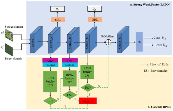
Figure 1.
The framework of the proposed method.
(a) Strong Weak Faster R-CNN: The method is inherited from Faster R-CNN; it narrows the domain shift at local and global levels by local discriminator and global discriminator . The gradient reversal layer (GRL) connects the domain discriminator with the feature extraction network to achieve adversarial training. We focused on the process of feature extraction, represented by a series of blue cuboids in Figure 1. For clarity, we briefly review the structure of the feature extraction network (taking ResNet-101 [56] as an example) here. As shown in Table 1, the blocks consist of a series of convolutional layers successively named Conv1, Conv2_x, Conv3_x, Conv4_x, and Conv5_x. Conv1~Conv4_x are responsible for extracting convolutional features of images from the source and target domains. Conv5_x is a region-of-interest (ROI)-based classifier. The loss function of the Strong Weak Faster R-CNN is composed of local-level adaptation loss , global-level adaptation loss , and the detection loss of Faster R-CNN .

Table 1.
Structure of ResNet101.
(b) Cascade RPNs: As shown in Figure 1, this module consists of three RPNs with the same structure; they are sequentially attached to Conv2_x, Con3_x, and Conv4_x of the Strong Weak Faster R-CNN to obtain multilevel features. Since the feature map from Conv4_x has a different size from that of from Conv2_x and Conv3_x, convolutional blocks composed of a convolutional layer and an average pooling layer are deployed between the RPN and Strong Weak Faster R-CNN pipeline for integration convenience. These multilevel features are fed into the corresponding RPN to generate proposals. Afterwards, the RPN classifier outputs binary classification probability for each proposal. The higher the probability value, the more likely there is a tree crown in the proposal. Then, we set a threshold value at each stage, the easy samples whose classification score is greater than or equal to the threshold are rejected at this stage and do not participate in the training of latter stages. The loss of cascade RPNs consists of three classification loss of all three RPNs and the regression loss of RPN3.
In this paper, we concentrated on the unsupervised DA tree-crown detection across two different regions. Specifically, we defined images from labeled source domain as , and images from unlabeled target domain as , where is the labels of , and and represent the number of images from the source domain and the target domain, respectively.
In the following sections, we explain the implementation of cascade RPNs, the integration details with Strong Weak Faster R-CNN and the filtering strategy successively.
3.1. Cascade Region Proposal Networks
As shown in Figure 1, images from the source domain and target domain are sequentially input into the feature extraction network, and these features are fed into the branch of cascade RPNs and generate a set of candidate regional proposals; the last layer of each branch outputs a classification probability between 0 and 1 with a softmax function for source proposals when training. Then, some easy samples from the source domain are filtered out if the probability is greater than a threshold, and the remaining samples go on to the training of the next cascade stage.
According to the green line of dashes in Figure 1, for example, the source image features extracted by Conv1 and Conv2_x are resized and fed into PRN1 and generate region proposals with corresponding binary classification scores. For training efficiency, 1024 of these region proposals are selected and used to train RPN1. If the proposal feature is significantly different from that of the real tree crown, it obtains a very high classification score in the background category in RPN1 and is then marked as the easiest negative sample and rejected. Similarly, the easiest positive samples is also filtered at this stage. Then, the same number of region proposals is generated in the deeper feature map further extracted by Conv3_x, but only 512 of the remaining harder samples are used to train RPN2, and the comparatively easier samples are rejected at that stage. Similar processes are applied in RPN3 with an extra bounding-box regression. Finally, the remaining proposals are allowed to join the subsequent processing.
Such a cascade structure brings two advantages:
(1) A large quantity of easy samples are detected and rejected at an early stage, which reduces the number of samples to be trained in the subsequent network and improves the computing efficiency of the network.
(2) In cascade RPNs, the classifiers perform a stage-by-stage hard sampling. Each RPN can be trained to detect the tree crown at different levels of difficulty. Consequently, the classifier of RPNs is sequentially adept at distinguishing more difficult distractors, and the distribution of training samples are sequentially more balanced.
As in Faster R-CNN, in Strong Weak Faster R-CNN, the RPN loss function is composed of binary classification loss function and regression loss function as Equation (1):
represents the probability that the ith anchor contains an object ( when the ith anchor box is positive, otherwise = 0). and are the trained coordinates of the anchor box and the coordinates of the ground-truth bounding box, respectively. is the proposal minibatch size for participating in the RPN training, and is the number of anchor locations. Specifically,
where R is a smooth L1 loss function.
Similar to the Strong Weak Faster R-CNN, in CAS-DA, the cascade RPNs adopt a multitask loss, including the binary classification loss in the () stage and the regression loss of the final stage. For each stage, the binary classification loss is computed as Equation (2). The regression loss is computed as Equation (3). The loss function of cascade RPNs is expressed as follows:
where = 1, R = 3, and r∈{1,2,3} in this paper. Similar to the Strong Weak Faster R-CNN, is a vector representing the classification score at stage r for the background and objects. is the minibatch size of the RPN, is the number of anchor locations of the final stage. Additionally, is introduced in CAS-DA to evaluates whether the sample is simple or not, it is a one-dimensional binary tensor (0 represents an easy sample, 1 represents a nonsimple sample) whose length is consistent with the number of anchor locations. Specifically, we set a threshold value (e.g., 0.99) at each stage and the ’s are all initialized to one, is 0 if the classification score is greater than the threshold, otherwise it is 1. The RPN randomly selects minibatch samples from the unrejected set for training. in a form of a successive multiplication means that, as long as a sample is rejected by any of the cascade stage, it will not have the opportunity to participate in the training of a later stage. Intuitively, the classification score of deep features counts more than that of shallow features, so is introduced to control the weight of the loss at different cascade stages and make sure losses from a deeper stage are attributed more weight. Specifically, the weight of the loss in the previous stage is one tenth that in the later stage. It can be seen that if R = = = 1, the item is a classical cross-entropy loss. Moreover, it is worth noting that the above procedure filters both simple positive and simple negative samples simultaneously, thus few simple positive samples are filtered at the early stage as well.
3.2. Integration with Strong Weak Faster R-CNN
We took the state-of-the-art Strong Weak Faster R-CNN as our baseline detector. Since CAS-DA focuses on strengthening the learning ability of RPN classifier, we only needed to add extra RPNs without making any changes to the other processes. The implementation details of CAS-DA are as follows: First, the structure and the data flow of RPN1 and RPN2 were designed similarly to those of the RPN in Strong Weak Faster R-CNN, i.e., RPN3 in Figure 1. To make sure that the feature maps with the same size were available for the three RPNs, we added convolutional blocks composed of a 1 × 1 convolutional layer and an average pooling layer between the first two cascade RPNs and the feature extractor. Specifically, the convolutional layer size was 1 × 1 × 1024, the pooling layer output feature map was 38 × 38, and finally, a feature map of 38 × 38 × 1024 was fed to RPNs. For the convenience of joint training, the batch size of each stage, i.e., (r∈{1,2,3}), was set to 1024, 512, and 256, respectively, in which the batch size of RPN3 was the same as that of the RPN in Strong Weak Faster R-CNN. Furthermore, a one-dimensional tensor, i.e., , was introduced to evaluate whether the sample was rejected in previous stages.
Finally, we can train our CAS-DA in an end-to-end manner by backward propagation. The training loss was designed to compose the loss of detection and domain adaptation, they were balanced by the trade-off parameter . Specifically:
where and are both composed of classification loss and regression loss.
3.3. A Filtering Strategy for Wrong Trees Based on Planting Rules
To further improve the precision of detection, we propose a filtering strategy based on the empirical planting rules of the tree crown, which can be applied to the postprocessing in validation and effectively filter the wrongly detected trees (false positives) by CAS-DA.
In large-scale tree-crown detection, we observed that most of the trees were planted together and distributed intensively; trees planted individually or in clusters of two or three are not abundantly found. In other words, there should be several (at least 2) other tree crowns around a tree crown within a certain range. Depending on this prerequisite, we propose a tree-crown filtration strategy.
First, we calculated the center of each bounding box classified as a tree crown by CAS-DA. If there were C bounding boxes, a matrix with the shape of C × C was generated, and the corresponding values represented the distance between two coordinates. It was stipulated that the detected tree crowns should be marked as false positives and dropped out if there were fewer than or exactly 2 detected trees within m pixels of them. As described above, the tree crowns are arranged intensively in remote sensing images, so m was set to the average size of the tree crown to obtain the best filtering effect. Specifically, m = 64 in dataset A and B (given that the size of a tree crown was about 64 × 64), and m = 75 in dataset C (given that the size of a tree crown was about 75 × 75). In Section 5.1.1, we explore the significance of this filtering strategy.
4. Experiments
4.1. Study Area and Dataset
In this research, the proposed method was applied to detect oil palm in remote sensing images from three different regions. As one of the major tropical cash crops in the world, the detection and counting of oil palm is of great significance to both economy and ecology.
As shown in Figure 2, we obtained two high-resolution satellite images (i.e., images A and B) in Peninsular Malaysia [44]. These two images were acquired at different times and places with different equipment, and therefore, they differed significantly in environmental conditions and resolution. Another remote sensing image (image C) was taken by a UAV in South Kalimantan, Indonesia [57]. Table 2 shows the elaborate information of the three images.
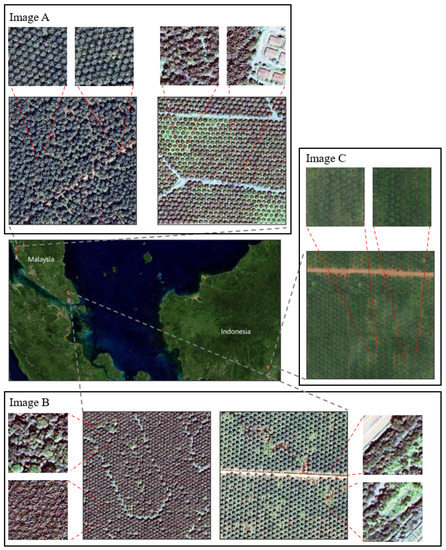
Figure 2.
The location of our study area and training examples used in this paper. We obtained images from three sets (i.e., (A–C)), the images randomly selected from the training region are arranged at the top, bottom, and right of the study area image, respectively.
Table 2.
The necessary information about image A, image B and image C.
In images A and B, there were four kinds of samples: background, oil palm, other vegetation, and the impervious background. The training datasets were collected from four regions of these two images, respectively. To evaluate the performance of our proposed method, we chose another representative region in images A and B as the validation datasets and compared the detected results with the ground truth collected by manual annotation. For images from training and validation regions, a bilinear interpolation was first applied to resize them to 2400 × 2400 pixels, and then the enlarged images were cropped randomly to 500 × 500 pixels. Finally, we obtained 4718 samples in image A and 3782 samples in image B.
In image C, in addition to the tree crown, there were also rivers, buildings, and other vegetation. The training datasets were from one region, and the validation datasets were from the other one. Since the images were originally collected for growing status observation by Jz et al. [57], there were more varieties in crown size and appearance compared with images A and B, such as small palm and yellowed palm. We firstly unified their labels into oil palm and then split the training region into 3148 images and the validation region into 851 images with 1024 × 1024 pixels.
Figure 2 shows the location of our study area and the examples of the training region from three locations. We can easily observe that the tree crowns distributed intensively and had a low category diversity. Table 3 shows information on the three datasets.
Table 3.
The necessary information on the datasets.
4.2. Experimental Setup and Evaluation Metrics
We applied the proposed method (CAS-DA + filtering) in two different domain-shift scenarios: (1) adaptations between images collected by satellites and UAVs, including dataset B → dataset C (B → C), dataset C → dataset B (C → B), dataset A → dataset C (A → C), and dataset C → dataset A (C → A); (2) adaptations between images collected by different satellites, including dataset A → dataset B (A → B) and dataset B → dataset A (B → A). Note that s → t above means adaptation from source domain to target domain.
We implemented our method based on PyTorch [58] on Ubuntu 18.04 using a GeForce RTX 1080 Ti. Our backbone network was ResNet-101 pretrained with Image-Net [59]. The network was trained with the backpropagation algorithm. The initial learning rate was 0.001, and it was divided by 10 every 50k iterations. Each batch included one image from the source domain and one image from the target domain. Conventionally, all images were resized to 600 × 600 after preprocessing. With this design, the feature maps from the three stages were resized to 38 × 38 × 1024 by the convolutional layer and pooling layer introduced in Section 3.2. For cascade RPNs, the threshold for an easy sample was set to 0.99 and = = 1. According to the size of tree crowns in our image, we defined the anchors to have a width of {64, 80} pixels and only assign a {1:1} aspect ratio considering that the shape of the tree crown was close to a square, which caused the number of anchor locations in an image (i.e., the length of ) to be fixed to 2888. For the loss function, we set the trade-off parameter = 0.1. Readers can refer to [40] for further details of the implementation of Strong Weak Faster R-CNN.
In validation, only the images from the target domain were used. We set the maximum number of tree crowns in an image to 100 and used NMS as the postprocessing method before the proposed filtering strategy.
We used true positive (TP), false positive (FP), false negative (FN), precision, recall, and F1-score as evaluation indicators. TP represents true positives, which is the number of crowns correctly detected. FP represents false negatives, referring to other objects mistaken for the crown. FN represents false negatives and denotes the number of crowns undetected. In our validation, the detecting results with a probability score over 0.5 and an IoU with the ground truth that was higher than 0.5 were considered to be TP. Precision indicates the proportion of correctly detected tree crowns in the detected tree crowns. Recall describes the proportion of correctly detected tree crowns in all ground-truth data. F1-score was introduced to balance these two indicators by computing their harmonic mean value.
4.3. Experiment Results
4.3.1. Experiments between Images Collected by Satellites and UAVs
Table 4 display the results of our proposed method (CAS-DA + filtering) in experiments between satellite images and UAV images. We can observe that our proposed method achieved 69.48%, 51.24%, 68.01%, and 87.06% in terms of F1-score on four transfer tasks; the average F1-score was 68.95%.
Table 4.
The detection results of our proposed method in experiment between satellite images and UAV images.
We also compared our proposed method with other methods, including F-RCNN (source) [9], DA Faster R-CNN [39], Strong Weak Faster R-CNN [40], CROPTD [45], and SW-ICR-CCR [41]. The results are shown in Table 5 and Table 6. F-RCNN (source) denotes Faster R-CNN trained only with source images and tested on the target images. Intuitively, a better performance of F-RCNN (source) implies a smaller gap in the feature distribution from the source domain to the target domain, i.e., a smaller domain shift. The other four are representative DA methods. For comparison fairness, the experiment setups of these methods were all as described in Section 4.2.
Table 5.
The detection results of different methods on B → C and C → B.
Table 6.
The detection results of different methods on A → C and C → A.
In this paper, the bold values in the table indicate the maximum value in the corresponding evaluation index unless noted otherwise.
Comparing the performance of these methods, a noteworthy phenomenon was the dramatic drop in the performance, especially the recall, of Strong Weak Faster R-CNN and CROPTD in B → C, C → B, and C → A, with average F1-scores of only 19.13% and 35.67%, respectively. There are three possible key reasons for this: (1) As mentioned in Section 4.1, dataset C was the only dataset collected by UAV, which exhibited a clear visual difference with the other two datasets in terms of image quality/resolution, texture, etc. The knowledge learned by CAS-DA on image C could not be well generalized to image A and image B, which was proved by the poor results of Faster RCNN (source) on C → B and C → A. On the contrary, Faster RCNN (source) achieved good performance (even better than DA F-RCNN) on A → C, indicating that the knowledge learned in dataset A could be directly transferred to dataset C to a certain extent. (2) In image C, there were palms in unhealthy growth status such as dead and yellowed ones that did not exist in image A and image B. Consequently, when C was taken as the target domain, these unhealthy palms were missed by the detector due to their difference from healthy ones in the source domain in terms of texture, size, etc., resulting in a decrease in recall. When we consider C as the source domain, these outlier features were prone to negative transfer, hurting the transferability of the model. (3) CROPTD is inherited from Strong Weak Faster R-CNN. Compared to other DA methods, both eliminated instance-level alignment, which also caused a performance decline, especially when there were a quantity of background samples similar to the object.
Our proposed method ranked at or near the top of the listed DA methods in terms of both precision and recall, thus achieving the highest F1-score in all four transfer experiments. Compared with Strong Weak Faster R-CNN (baseline), our method showed a greater robustness and improved the F1-score on the four experiments by 5.61%~58.75%.
To demonstrate the experimental results more clearly, Table 7 shows the F1-scores of all methods in the four experiments. Our proposed method achieved the best performance with 68.95% in terms of average F1-score, outperforming DA F-RCNN, Strong Weak Faster R-CNN, CROPTD, and SW ICR-CCR by an obvious margin of 11.88%, 40.00%, 12.36%, and 26.01%, respectively.
Table 7.
The F1-scores of different methods on four transfer tasks.
We divided the experimental results from Table 7 into two groups: adaptation between dataset B and dataset C (i.e., B ↔ C, including B → C and C → B), and adaptation between dataset A and dataset C (i.e., A ↔ C, including A → C and C → A). We noticed that the performance of Faster RCNN (source) in B ↔ C was clearly worse than that in A ↔ C. Combined with the previously mentioned results, we can draw the conclusion that the domain shift between B and C was more significant than that between A and C, which was also confirmed by the experimental results of the DA methods: taking C as the source domain, in C → B and C → A, all of the DA methods obtained the worst performance in C → B, and our method also achieved an F1-score of only 51.24%, while in C → A, they performed much better, and our method achieved an F1-score of 87.06%.
Analyzing these two groups of experiments from another perspective, it can be seen that our method led to a more remarkable improvement of the adaptation with a larger domain shift. Specifically, compared with the other four DA methods, our method improved the average F1-score of B ↔ C by 11.32%~45.82%, exceeding 10.97~32.18% on A↔C. It proved that our method, which focuses on improving classification capability on source domain, was more effective than the other DA methods that focus on diminishing the domain shift across common benchmarks, especially in the presence of a large domain shift.
4.3.2. Experiments between Images Collected by Different Satellites
To further verify the effectiveness of the proposed method, we performed adaptation between two high-resolution satellite images. The experimental results are shown in Table 8, Table 9 and Table 10.
Table 8.
The detection results of our proposed method between images collected by different satellites.
Table 9.
The detection results of different methods on A → B and B → A.
Table 10.
The F1-scores of different methods on two transfer tasks.
TP, FP, FN, precision, recall, and F1-score for A → B and B → A are listed in Table 2. Our proposed method achieved an F1-score of 82.95% in A → B and 94.70% in B → A.
As shown in Table 9 and Table 10, it is noticed that not all DA methods outperformed F-RCNN (source). For example, the performance of DA F-RCNN on A → B was worse than that of F-RCNN (source). Our proposed method achieved the best performance on two transfer tasks, with F1-scores of 3.29 and 2.16 percentage points higher than Strong Weak Faster R-CNN (baseline) in two experiments. The average F1-score was 88.83%, outperforming other DA methods by 5.02%, 2.73%, 0.80%, and 0.50%. Furthermore, the good performance of F-RCNN (source) implied a smaller domain shift between A and B than that in the previous adaptation scenario.
To summarize Section 4.3.1 and Section 4.3.2: (1) The performance of all DA methods between different satellite images (as shown in Table 10) was superior to that between satellite images and UAV images (as shown in Table 7), which might be because the significant domain shift in the latter brought a greater difficulty for the DA detector to learn the domain-invariant features. (2) Compared to the other DA methods that focus on diminishing the domain-shift, our method obtained the highest F1-score in two different adaptation scenarios. which demonstrates the importance and effectiveness of improving the detection performance on the source domain to enhance the DA detector. Moreover, it is worth noting that our method brought a greater improvement for the adaptation with a large domain shift.
5. Discussion
5.1. Ablation Study
5.1.1. Effects of Filtering Strategy
In order to verify the effectiveness of the filtering strategy, we evaluated the performance of the filtering strategy on B → C, C → B, A → C, C → A, A → B, and B → A. The experimental results in Table 11, Table 12, Table 13, Table 14, Table 15 and Table 16 prove that adding filtering strategy helped filter out wrongly detected trees effectively as it improved the F1-score by 0.85%, 0.25%, 0.07%, 0.58%, 0.57%, and 0.18% on six transfer experiments, respectively.
Table 11.
Effects of the filtering strategy on B → C.
Table 12.
Effects of the filtering strategy on C → B.
Table 13.
Effects of the filtering strategy on A → C.
Table 14.
Effects of the filtering strategy on C → A.
Table 15.
Effects of the filtering strategy on A → B.
Table 16.
Effects of the filtering strategy on B → A.
Moreover, there was a slightly decrease in TP and precision after filtering since a few individual trees were correctly detected but filtered by mistake. Despite all of this, Table 11, Table 12, Table 13, Table 14, Table 15 and Table 16 reveal that 972, 814, 377, 504, 569, and 269 detected trees were dropped through the filtering process, of which 588, 636, 288, 459, 522, and 171 were false positives while only 384, 178, 89, 45, 47, and 98 were true positives, which improved the F1-score by increasing the precision of the detection.
5.1.2. Effects of Cascade Stages
Table 17, Table 18 and Table 19 summarize the performance of our CAS-DA method with a different number of cascade stages. SW is an abbreviation for Strong Weak Faster RCNN that only uses RPN3.
Table 17.
Effects of cascade stages on B → C and C → B. The best F1-score was reached when three RPNs were added.
Table 18.
Effects of cascade stages on A → C and C → A. The best F1-score was reached when three RPNs were added.
Table 19.
Effects of cascade stages on A → B and B → A. The best F1-score was reached when three RPNs were added.
Here are our observations: (1) SW achieved the worst F1-score in all experiments when no cascade RPN was added. (2) By adding RPN1 or RPN2, the detector outperformed SW. Specifically, adding RPN1 alone brought 47.52%, 26.18%, 4.45%, 28.47%, 1.64%, and 1.69% gains in F1-score and only adding RPN2 improved the F1-score by 46.68%, 23.98%, 1.18%, 3.36%, 0.72%, and 1.33%. However, adding either RPN1 or RPN2 still fell short of the best F1-score. (3) It is worth noting that RPN1 was more effective than RPN2 in all six experiments. This is possibly because a large number of very easy samples could be filtered in RPN1 using the shallow-level features. To prove it, we observed the training process and found that the number of easy samples filtered by RPN1 was always much more than that of RPN2. Taking A → B as an example, RPN1 generated 2888 anchors; after that, RPN1, RPN2, and RPN3 classified 1002, 418, and 22 of them as easy samples, respectively. (4) CAS-DA achieved the optimal performance when three RPNs were added at the same time, outperforming SW on six transfer tasks by 2.72%, 1.98%, 30.17%, 49.84%, 58.17%, and 5.54% in terms of F1-score, respectively, without the filtering strategy. More cascade stages may further improve the performance of the model but will also increase the cost of computing.
5.2. Easy-Sample Threshold Analysis
The smaller the threshold, the more samples may be filtered as easy samples by the cascade RPNs. Taking B → A as an example, we implemented the experiment with threshold values of 0.95, 0.96, 0.97, 0.98, 0.99, 0.999, and 0.9999. The results are shown in Figure 3.
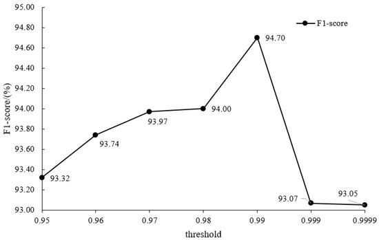
Figure 3.
F1-score of B → A with different threshold values. CAS-DA achieved the best F1-score when the threshold was set to 0.99.
When the threshold was less than or equal to 0.99, the cascade RPNs filtered out easy samples and improved the performance of the classifier, and the F1-score increased with the increase of the threshold. When the threshold was greater than 0.99, only a few samples were filtered, and the F1-score decreased significantly. Therefore, we finally selected 0.99 as the easy-sample threshold to obtain the highest F1-score.
5.3. Visualization and Analyses
5.3.1. Detection Examples
For visualization purpose, six example regions for the above experiments are illustrated in Figure 4, Figure 5, Figure 6, Figure 7, Figure 8 and Figure 9. The green rectangle represents the correctly detected crown (TP) and the red rectangle represents the backgrounds identified as crowns by mistake (FP). From top left to bottom right, the corresponding methods are the manually annotated ground truth, Strong Weak Faster R-CNN, CAS-DA, and CAS-DA with the filtering strategy, respectively.
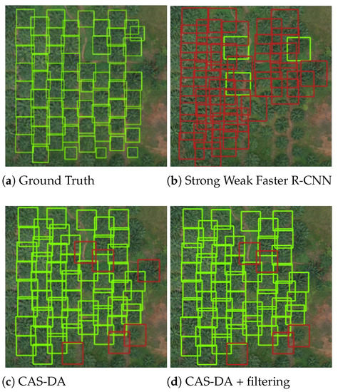
Figure 4.
Qualitative results for different methods on B → C.
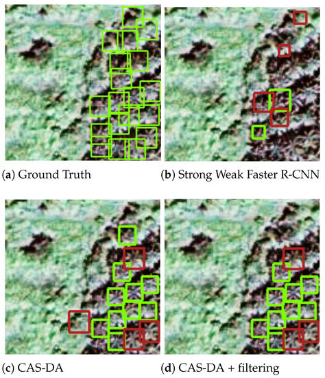
Figure 5.
Qualitative results for different methods on C → B.
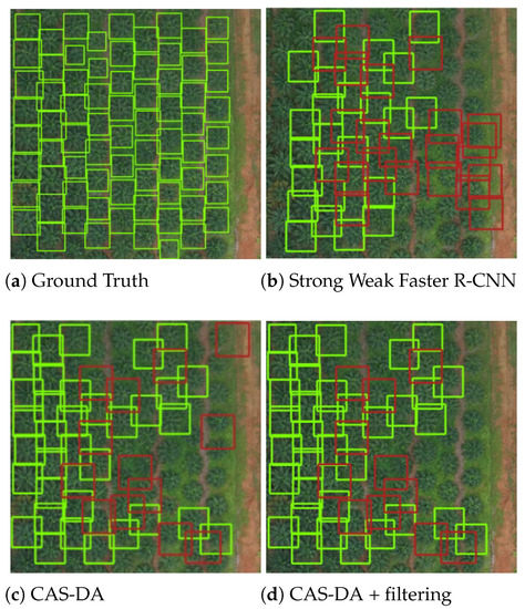
Figure 6.
Qualitative results for different methods on A → C.
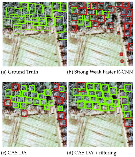
Figure 7.
Qualitative results for different methods on C → A.
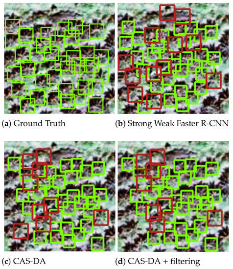
Figure 8.
Qualitative results for different methods on A → B.
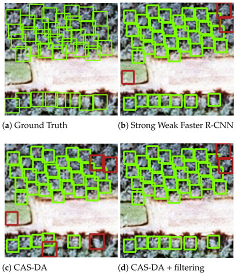
Figure 9.
Qualitative results for different methods on B → A.
The results demonstrate that CAS-DA outperformed Strong Weak Faster R-CNN in all six transfer tasks. In the detection results, the number of true positives (green rectangles) increased while the number of false positives (red rectangle) decreased. In addition, as shown in subimages (c) and (d), the wrongly detected trees (marked by red rectangles) were effectively removed by the proposed filtering strategy, which contributed to further improving the detection precision.
5.3.2. Response Map Visualization
In cascade RPNs, since the easy samples were rejected stage by stage, the RPN classifier was sequentially more discriminative in distinguishing tree crown from background or other difficult distractors. Figure 10 shows the response map activated by the ReLU function in each stage. Images from top to bottom come from datasets A, B, and C, respectively. We illustrate from left to right the ground truth and the response maps obtained by the RPN in the three stages. We can see that the RPN was sequentially more discriminative, and the tree crowns were localized more accurately.
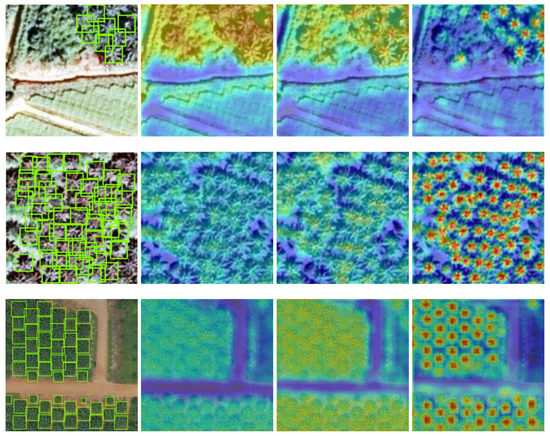
Figure 10.
Response maps in different RPN stages. RPN is sequentially more discriminative, and the tree crowns are localized more accurately.
6. Conclusions
In this paper, we proposed an end-to-end DA detector with cascade RPNs (i.e., CAS-DA) to realize the cross-regional tree-crown detection and counting. To deal with the problems of a poor abundance of objects and the data imbalance in tree-crown detection, the cascade RPNs were designed to adopt multiple region proposal networks to filter out easy samples so that the learning ability of deeper classifiers was gradually enhanced. Then, the adaptation components and detector were integrated to form an end-to-end framework for the cross-regional detection. In addition, a practical filtering method was proposed according to the observed tree-crown distribution rules to effectively eliminate the wrongly detected trees. Experiments in two different adaptation scenarios showed that our method achieved 68.95% and 88.83% average F1-scores, respectively, significantly outperforming the other DA approaches focusing on diminishing the domain shift across common benchmarks, showing its effectiveness in cross-domain tree-crown detection using remote sensing images. Particularly, our method obtained a greater performance boost for the adaption with a larger domain shift. From the experimental results, we could draw the conclusion that, in tree-crown detection, it is more effective to improve the detection performance on the source domain than to diminish the domain shift, especially when confronted with a significant domain shift.
Moreover, our method has the potential to realize other DA object detection with similar characteristics to overcome the scarcity of labeled data and the difficulty of traditional deep learning methods in transfer learning across different domains. For example, in the remote sensing field, it can be directly applied to the cross-regional growing-status observation of the same tree species after labeling the source domain with fine-grained labels. Furthermore, fault detection in different environments, such as the fault detection of mechanical equipment, high-voltage line, etc., is also a possible scenario, where the forms of the fault are few and the image background is very complex, limiting the performance of traditional RPN-based detector. Introducing DA methods with cascade RPNs could be beneficial by saving labeling costs and locating the fault more precisely.
Nevertheless, there is still much room for improving the performance of cross-domain detection between satellite images and UAV images due to the great difference in styles, textures, etc. Therefore, we hope to build a more effective cross-domain tree-crown detector for this adaptation in the future.
Author Contributions
Methodology, Y.W. and G.Y.; writing—original draft preparation, Y.W.; writing—review and editing, G.Y. and H.L. All authors have read and agreed to the published version of the manuscript.
Funding
This work was supported in part by the National Key Research and Development Program of China (grant no. 2020YFE0200800) and the National Natural Science Foundation of China (grant no. 42001376).
Institutional Review Board Statement
Not applicable.
Informed Consent Statement
Not applicable.
Data Availability Statement
Not applicable.
Conflicts of Interest
The authors declare no conflict of interest.
References
- Dalponte, M.; Ørka, H.O.; Ene, L.T.; Gobakken, T.; Næsset, E. Tree crown delineation and tree species classification in boreal forests using hyperspectral and ALS data. Remote Sens. Environ. 2014, 140, 306–317. [Google Scholar] [CrossRef]
- Wang, Y.; Zhu, X.; Wu, B. Automatic detection of individual oil palm trees from UAV images using HOG features and an SVM classifier. Int. J. Remote Sens. 2019, 40, 7356–7370. [Google Scholar] [CrossRef]
- Pu, R.; Landry, S. A comparative analysis of high spatial resolution IKONOS and WorldView-2 imagery for mapping urban tree species. Remote Sens. Environ. 2012, 124, 516–533. [Google Scholar] [CrossRef]
- Hung, C.; Bryson, M.; Sukkarieh, S. Multi-class predictive template for tree crown detection. ISPRS J. Photogramm. Remote Sens. 2012, 68, 170–183. [Google Scholar] [CrossRef]
- Wang, X.; Li, L.; Ye, W.; Long, M.; Wang, J. Transferable Attention for Domain Adaptation. In Proceedings of the AAAI Conference on Artificial Intelligence, Honolulu, HI, USA, 27 January–1 February 2019; Volume 33, pp. 5345–5352. [Google Scholar]
- Wang, M.; Deng, W. Deep Visual Domain Adaptation: A Survey. Neurocomputing 2018, 312, 135–153. [Google Scholar] [CrossRef]
- Everingham, M.; Van Gool, L.; Williams, C.K.; Winn, J.; Zisserman, A. The pascal visual object classes (voc) challenge. Int. J. Comput. Vis. 2009, 88, 303–308. [Google Scholar] [CrossRef]
- Lin, T.Y.; Maire, M.; Belongie, S.; Hays, J.; Perona, P.; Ramanan, D.; Dollár, P.; Zitnick, C.L. Microsoft coco: Common objects in context. In Proceedings of the Computer Vision–ECCV 2014: 13th European Conference, Zurich, Switzerland, 6–12 September 2014; Springer: Berlin/Heidelberg, Germany, 2014; pp. 740–755. [Google Scholar]
- Ren, S.; He, K.; Girshick, R.; Sun, J. Faster r-cnn: Towards real-time object detection with region proposal networks. Adv. Neural Inf. Process. Syst. 2015, 28. Available online: https://proceedings.neurips.cc/paper_files/paper/2015/file/14bfa6bb14875e45bba028a21ed38046-Paper.pdf (accessed on 17 June 2023). [CrossRef]
- Lin, T.Y.; Dollár, P.; Girshick, R.; He, K.; Hariharan, B.; Belongie, S. Feature pyramid networks for object detection. In Proceedings of the IEEE Conference on Computer Vision and Pattern Recognition, Honolulu, HI, USA, 21–26 July 2017; pp. 2117–2125. [Google Scholar]
- Liu, W.; Anguelov, D.; Erhan, D.; Szegedy, C.; Reed, S.; Fu, C.Y.; Berg, A.C. Ssd: Single shot multibox detector. In Proceedings of the Computer Vision–ECCV 2016: 14th European Conference, Amsterdam, The Netherlands, 11–14 October 2016; Springer: Berlin/Heidelberg, Germany, 2016; pp. 21–37. [Google Scholar]
- Redmon, J.; Divvala, S.; Girshick, R.; Farhadi, A. You only look once: Unified, real-time object detection. In Proceedings of the IEEE Conference on Computer Vision and Pattern Recognition, Las Vegas, NV, USA, 26 June–1 July 2016; pp. 779–788. [Google Scholar]
- Shrivastava, A.; Gupta, A.; Girshick, R. Training region-based object detectors with online hard example mining. In Proceedings of the IEEE Conference on Computer Vision and Pattern Recognition, Las Vegas, NV, USA, 26 June–1 July 2016; pp. 761–769. [Google Scholar]
- Lin, T.Y.; Goyal, P.; Girshick, R.; He, K.; Dollár, P. Focal loss for dense object detection. In Proceedings of the IEEE International Conference on Computer Vision, Venice, Italy, 22–29 October 2017; pp. 2980–2988. [Google Scholar]
- Pang, J.; Chen, K.; Shi, J.; Feng, H.; Ouyang, W.; Lin, D. Libra R-CNN: Towards Balanced Learning for Object Detection. In Proceedings of the 2019 IEEE/CVF Conference on Computer Vision and Pattern Recognition (CVPR), Long Beach, CA, USA, 15–20 June 2019; pp. 821–830. [Google Scholar]
- Gidaris, S.; Komodakis, N. Attend refine repeat: Active box proposal generation via in-out localization. arXiv 2016, arXiv:1606.04446. [Google Scholar]
- Wang, J.; Chen, K.; Yang, S.; Loy, C.C.; Lin, D. Region proposal by guided anchoring. In Proceedings of the IEEE/CVF Conference on Computer Vision and Pattern Recognition, Long Beach, CA, USA, 15–20 June 2019; pp. 2965–2974. [Google Scholar]
- Zhong, Q.; Li, C.; Zhang, Y.; Xie, D.; Yang, S.; Pu, S. Cascade Region Proposal and Global Context for Deep Object Detection. arXiv 2017, arXiv:1710.10749. [Google Scholar] [CrossRef]
- Vu, T.; Jang, H.; Pham, T.X.; Yoo, C.D. Cascade RPN: Delving into High-Quality Region Proposal Network with Adaptive Convolution. In Proceedings of the Neural Information Processing Systems, Vancouver, BC, Canada, 8–14 December 2019. [Google Scholar]
- Cho, M.; Chung, T.Y.; Lee, H.; Lee, S. N-RPN: Hard Example Learning For Region Proposal Networks. In Proceedings of the 2019 IEEE International Conference on Image Processing (ICIP), Taipei, Taiwan, 22–25 September 2019; pp. 3955–3959. [Google Scholar]
- Daliakopoulos, I.N.; Grillakis, E.G.; Koutroulis, A.G.; Tsanis, I.K. Tree crown detection on multispectral VHR satellite imagery. Photogramm. Eng. Remote Sens. 2009, 75, 1201–1211. [Google Scholar] [CrossRef]
- Wulder, M.; Niemann, K.O.; Goodenough, D.G. Local maximum filtering for the extraction of tree locations and basal area from high spatial resolution imagery. Remote Sens. Environ. 2000, 73, 103–114. [Google Scholar] [CrossRef]
- Pouliot, D.; King, D.; Bell, F.; Pitt, D. Automated tree crown detection and delineation in high-resolution digital camera imagery of coniferous forest regeneration. Remote Sens. Environ. 2002, 82, 322–334. [Google Scholar] [CrossRef]
- Krizhevsky, A.; Sutskever, I.; Hinton, G.E. Imagenet classification with deep convolutional neural networks. Commun. ACM 2017, 60, 84–90. [Google Scholar] [CrossRef]
- Li, W.; Fu, H.; Yu, L.; Cracknell, A. Deep learning based oil palm tree detection and counting for high-resolution remote sensing images. Remote Sens. 2016, 9, 22. [Google Scholar] [CrossRef]
- Mubin, N.A.; Nadarajoo, E.; Shafri, H.Z.M.; Hamedianfar, A. Young and mature oil palm tree detection and counting using convolutional neural network deep learning method. Int. J. Remote Sens. 2019, 40, 7500–7515. [Google Scholar] [CrossRef]
- Neupane, B.; Horanont, T.; Hung, N.D. Deep learning based banana plant detection and counting using high-resolution red-green-blue (RGB) images collected from unmanned aerial vehicle (UAV). PLoS ONE 2019, 14, e0223906. [Google Scholar] [CrossRef]
- Li, W.; Dong, R.; Fu, H.; Yu, L. Large-scale oil palm tree detection from high-resolution satellite images using two-stage convolutional neural networks. Remote Sens. 2018, 11, 11. [Google Scholar] [CrossRef]
- Zheng, J.; Li, W.; Xia, M.; Dong, R.; Fu, H.; Yuan, S. Large-scale oil palm tree detection from high-resolution remote sensing images using faster-rcnn. In Proceedings of the IGARSS 2019–2019 IEEE International Geoscience and Remote Sensing Symposium, Yokohama, Japan, 28 July–2 August 2019; IEEE: Piscataway, NJ, USA, 2019; pp. 1422–1425. [Google Scholar]
- Feng, X.; Li, P. A tree species mapping method from UAV images over urban area using similarity in tree-crown object histograms. Remote Sens. 2019, 11, 1982. [Google Scholar] [CrossRef]
- Santos, A.A.d.; Marcato Junior, J.; Araújo, M.S.; Di Martini, D.R.; Tetila, E.C.; Siqueira, H.L.; Aoki, C.; Eltner, A.; Matsubara, E.T.; Pistori, H.; et al. Assessment of CNN-based methods for individual tree detection on images captured by RGB cameras attached to UAVs. Sensors 2019, 19, 3595. [Google Scholar] [CrossRef]
- Puttemans, S.; Van Beeck, K.; Goedemé, T. Comparing boosted cascades to deep learning architectures for fast and robust coconut tree detection in aerial images. In Proceedings of the 13th International Joint Conference on Computer Vision, Imaging and Computer Graphics Theory and Applications, SCITEPRESS, Madeira, Portugal, 27–29 January 2018; Volume 5, pp. 230–241. [Google Scholar]
- Tzeng, E.; Hoffman, J.; Zhang, N.; Saenko, K.; Darrell, T. Deep domain confusion: Maximizing for domain invariance. arXiv 2014, arXiv:1412.3474. [Google Scholar]
- Wang, X.; Jin, Y.; Long, M.; Wang, J.; Jordan, M.I. Transferable normalization: Towards improving transferability of deep neural networks. Adv. Neural Inf. Process. Syst. 2019, 32, 1953–1963. [Google Scholar]
- Zhang, Y.; David, P.; Gong, B. Curriculum domain adaptation for semantic segmentation of urban scenes. In Proceedings of the IEEE International Conference on Computer Vision, Venice, Italy, 22–29 October 2017; pp. 2020–2030. [Google Scholar]
- Hoffman, J.; Tzeng, E.; Park, T.; Zhu, J.Y.; Isola, P.; Saenko, K.; Efros, A.; Darrell, T. Cycada: Cycle-consistent adversarial domain adaptation. In Proceedings of the International Conference on Machine Learning, Stockholm, Sweden, 10–15 July 2018; pp. 1989–1998. [Google Scholar]
- Ghifary, M.; Kleijn, W.; Zhang, M. Domain Adaptive Neural Networks for Object Recognition. In Proceedings of the Pacific Rim International Conference on Artificial Intelligence, Gold Coast, QLD, Australia, 1–5 December 2014. [Google Scholar]
- Shi, Y.; Li, L.; Yang, J.; Wang, Y.; Hao, S. Center-based Transfer Feature Learning With Classifier Adaptation for surface defect recognition. Mech. Syst. Signal Process. 2023, 188, 110001. [Google Scholar] [CrossRef]
- Chen, Y.; Li, W.; Sakaridis, C.; Dai, D.; Van Gool, L. Domain adaptive faster r-cnn for object detection in the wild. In Proceedings of the IEEE Conference on Computer Vision and Pattern Recognition, Salt Lake City, UT, USA, 18–23 June 2018; pp. 3339–3348. [Google Scholar]
- Saito, K.; Ushiku, Y.; Harada, T.; Saenko, K. Strong-weak distribution alignment for adaptive object detection. In Proceedings of the IEEE/CVF Conference on Computer Vision and Pattern Recognition, Long Beach, CA, USA, 15–20 June 2019; pp. 6956–6965. [Google Scholar]
- Xu, C.D.; Zhao, X.R.; Jin, X.; Wei, X.S. Exploring categorical regularization for domain adaptive object detection. In Proceedings of the IEEE/CVF Conference on Computer Vision and Pattern Recognition, Seattle, WA, USA, 13–19 June 2020; pp. 11724–11733. [Google Scholar]
- Arruda, V.F.; Paixão, T.M.; Berriel, R.; de Souza, A.F.; Badue, C.S.; Sebe, N.; Oliveira-Santos, T. Cross-Domain Car Detection Using Unsupervised Image-to-Image Translation: From Day to Night. In Proceedings of the 2019 International Joint Conference on Neural Networks (IJCNN), Budapest, Hungary, 14–19 July 2019; pp. 1–8. [Google Scholar]
- Guo, T.; Huynh, C.P.; Solh, M. Domain-Adaptive Pedestrian Detection in Thermal Images. In Proceedings of the 2019 IEEE International Conference on Image Processing (ICIP), Taipei, Taiwan, 22–25 September 2019; pp. 1660–1664. [Google Scholar]
- Koga, Y.; Miyazaki, H.; Shibasaki, R. A method for vehicle detection in high-resolution satellite images that uses a region-based object detector and unsupervised domain adaptation. Remote Sens. 2020, 12, 575. [Google Scholar] [CrossRef]
- Wu, W.; Zheng, J.; Fu, H.; Li, W.; Yu, L. Cross-regional oil palm tree detection. In Proceedings of the IEEE/CVF Conference on Computer Vision and Pattern Recognition Workshops, Seattle, WA, USA, 13–19 June 2020; pp. 56–57. [Google Scholar]
- Zheng, J.; Fu, H.; Li, W.; Wu, W.; Zhao, Y.; Dong, R.; Yu, L. Cross-regional oil palm tree counting and detection via a multi-level attention domain adaptation network. ISPRS J. Photogramm. Remote Sens. 2020, 167, 154–177. [Google Scholar] [CrossRef]
- Felzenszwalb, P.F.; Girshick, R.B.; McAllester, D. Cascade object detection with deformable part models. In Proceedings of the 2010 IEEE Computer Society Conference on Computer Vision and Pattern Recognition, San Francisco, CA, USA, 13–18 June 2010; IEEE: Piscataway, NJ, USA, 2010; pp. 2241–2248. [Google Scholar]
- Shelhamer, E.; Long, J.; Darrell, T. Fully convolutional networks for semantic segmentation. In Proceedings of the 2015 IEEE Conference on Computer Vision and Pattern Recognition (CVPR), Boston, MA, USA, 7–12 June 2015; pp. 3431–3440. [Google Scholar]
- Xiao, R.; Zhu, L.; Zhang, H.J. Boosting chain learning for object detection. In Proceedings of the Ninth IEEE International Conference on Computer Vision, Nice, France, 13–16 October 2003; IEEE: Piscataway, NJ, USA, 2003; pp. 709–715. [Google Scholar]
- Yang, B.; Yan, J.; Lei, Z.; Li, S.Z. Craft objects from images. In Proceedings of the IEEE Conference on Computer Vision and Pattern Recognition, Las Vegas, NV, USA, 26 June–1 July 2016; pp. 6043–6051. [Google Scholar]
- Xu, Y.; Zhu, M.; Li, S.; Feng, H.; Ma, S.; Che, J. End-to-End Airport Detection in Remote Sensing Images Combining Cascade Region Proposal Networks and Multi-Threshold Detection Networks. Remote. Sens. 2018, 10, 1516. [Google Scholar] [CrossRef]
- Neubeck, A.; Van Gool, L. Efficient non-maximum suppression. In Proceedings of the 18th International Conference on Pattern Recognition (ICPR’06), Hong Kong, 20–24 August 2006; IEEE: Piscataway, NJ, USA, 2006; Volume 3, pp. 850–855. [Google Scholar]
- Qin, H.; Yan, J.; Li, X.; Hu, X. Joint training of cascaded CNN for face detection. In Proceedings of the IEEE Conference on Computer Vision and Pattern Recognition, Las Vegas, NV, USA, 26 June–1 July 2016; pp. 3456–3465. [Google Scholar]
- Fan, H.; Ling, H. Siamese Cascaded Region Proposal Networks for Real-Time Visual Tracking. In Proceedings of the 2019 IEEE/CVF Conference on Computer Vision and Pattern Recognition (CVPR), Long Beach, CA, USA, 15 June–20 June 2019; pp. 7944–7953. [Google Scholar]
- Zhang, X.; Fan, X.; Luo, S. Cascaded Region Proposal Networks for Proposal-Based Tracking. In Proceedings of the International Conference on Smart Multimedia, San Diego, CA, USA, 16–18 December 2019. [Google Scholar]
- He, K.; Zhang, X.; Ren, S.; Sun, J. Deep residual learning for image recognition. In Proceedings of the IEEE Conference on Computer Vision and Pattern Recognition, Las Vegas, NV, USA, 27–30 June 2016; pp. 770–778. [Google Scholar]
- Zheng, J.; Fu, H.; Li, W.; Wu, W.; Yu, L.; Yuan, S.; Tao, W.Y.W.; Pang, T.K.; Kanniah, K.D. Growing status observation for oil palm trees using Unmanned Aerial Vehicle (UAV) images. ISPRS J. Photogramm. Remote Sens. 2021, 173, 95–121. [Google Scholar] [CrossRef]
- Paszke, A.; Gross, S.; Massa, F.; Lerer, A.; Bradbury, J.; Chanan, G.; Killeen, T.; Lin, Z.; Gimelshein, N.; Antiga, L.; et al. Pytorch: An imperative style, high-performance deep learning library. Adv. Neural Inf. Process. Syst. 2019, 32, 8024–8035. [Google Scholar]
- Deng, J.; Dong, W.; Socher, R.; Li, L.J.; Li, K.; Fei-Fei, L. Imagenet: A large-scale hierarchical image database. In Proceedings of the 2009 IEEE Conference on Computer Vision and Pattern Recognition, Miami, FL, USA, 20–25 June 2009; IEEE: Piscataway, NJ, USA, 2009; pp. 248–255. [Google Scholar]
Disclaimer/Publisher’s Note: The statements, opinions and data contained in all publications are solely those of the individual author(s) and contributor(s) and not of MDPI and/or the editor(s). MDPI and/or the editor(s) disclaim responsibility for any injury to people or property resulting from any ideas, methods, instructions or products referred to in the content. |
© 2023 by the authors. Licensee MDPI, Basel, Switzerland. This article is an open access article distributed under the terms and conditions of the Creative Commons Attribution (CC BY) license (https://creativecommons.org/licenses/by/4.0/).