Abstract
We present a novel nonparametric adaptive partitioning and stitching (NAPS) algorithm to estimate a probability density function (PDF) of a single variable. Sampled data is partitioned into blocks using a branching tree algorithm that minimizes deviations from a uniform density within blocks of various sample sizes arranged in a staggered format. The block sizes are constructed to balance the load in parallel computing as the PDF for each block is independently estimated using the nonparametric maximum entropy method (NMEM) previously developed for automated high throughput analysis. Once all block PDFs are calculated, they are stitched together to provide a smooth estimate throughout the sample range. Each stitch is an averaging process over weight factors based on the estimated cumulative distribution function (CDF) and a complementary CDF that characterize how data from flanking blocks overlap. Benchmarks on synthetic data show that our PDF estimates are fast and accurate for sample sizes ranging from to , across a diverse set of distributions that account for single and multi-modal distributions with heavy tails or singularities. We also generate estimates by replacing NMEM with kernel density estimation (KDE) within blocks. Our results indicate that NAPS(NMEM) is the best-performing method overall, while NAPS(KDE) improves estimates near boundaries compared to standard KDE.
1. Introduction
In many domains, such as climate science, epidemiology, quality assurance, finance, and market analysis, there is a need for robust high throughput probability density estimation as the amount of information processed grows. The motivation for this work is to address the computational challenges of a reliable automated method that makes fast and accurate density estimates on massive datasets. If an application is limited to similar types of input data, expert domain knowledge can be used to develop appropriate models and limit the number of relevant parameters and their accessible range. However, high throughput analysis and turnkey automation are critical for large datasets, to relieve analysts from looking at each density estimate on an individual basis to either determine a reasonable parametric model to use, or to verify if a nonparametric model presents a reasonable solution. In this context, kernel density estimation (KDE) is arguably the most common approach for nonparametric density estimation.
A major contributing factor to the popularity of KDE is the intuitive interpretation of local binning and smoothing of observed data. The implementation of this conceptual idea using a simple Gaussian kernel to approximate each bin is straightforward [1,2,3,4,5,6]. However, it becomes readily apparent that there is a trade-off between smoothness in low density regions and accurate modeling of sharp features within the ground truth. Addressing this basic trade-off has created a long history of methodological and computational improvements over many decades of active research [7,8,9,10,11,12,13]. Despite its popularity, however, KDE suffers from two inherent weaknesses: the user must select both an optimal bandwidth for resolution of the estimate and an appropriate kernel for modeling boundary conditions accurately. With insight and knowledge of the expected results, the two weaknesses of KDE can be largely mitigated in practice. Unfortunately, KDE does not automatically work on any type of distribution without subjective selection options set by a human during a setup process. Furthermore, there is danger that if prior conditions change in high throughput applications, the user’s assumptions can become invalid, creating a risk for large errors.
There is a wide range of KDE methods available for data-driven adaptive bandwidths or adaptive kernel selection. However, these methods often incur substantial computational costs, especially when applied towards large data sets and often still require guidance by domain experts. As data demands increase in various applications, parallel computing methods for density estimation have been developed to employ multiple processors and resources, aiming to expedite the calculations [14,15,16,17,18,19,20]. The conceptual ideas of parallel processing also extend to multivariate density estimation, and several parallel computing implementations have been developed for higher dimensions [21,22,23]. Given the inherent parallelizability of the KDE, this method is a natural choice for breaking up the problem. Although parallel KDE implementations offer improved computational performance, they nevertheless suffer from the same inherent weaknesses of the underlying algorithm.
As an alternative to KDE, a fully automated method for univariate probability density estimation was introduced by JF and DJJ in 2018 [24]. With successive improvements since, open software packages in MATLAB, C++, Java, and R are now available [25,26]. Our data-adaptive model-free method requires no prior knowledge of the input data characteristics, therefore the user need not set the bandwidth nor any additional parameters. Our method is based on a maximum entropy principle, while solving an inverse problem using a trial cumulative probability function by optimizing an objective function that involves sort order statistics to obtain sampled uniform random data (SURD) [24]. We will refer to this base method as NMEM for nonparametric maximum entropy method.
The fundamental idea behind any maximum entropy method (MEM) is to generate a density estimate that remains non-committal to missing information based on partial knowledge, typically expressed through constraints on expectation values of specific functions. MEM aims to shape the probability density to match these constraints while being as spread out as possible, resulting in more accurate estimates in regions with missing data [27]. However, to improve accuracy near sharp features, simply adding more constraints can lead to reduced smoothness [28]. The challenge lies in determining the optimal balance between adding objective constraints for improved accuracy without introducing excessive bias due to overfitting, often through empirical estimation of constraints [29,30]. Thus, the problems of bandwidth and resolution in KDE methods are transferred to a different problem involving finding the most appropriate set of constraints in MEM. Both KDE and MEM require the user to input domain knowledge to ensure robust results.
Our NMEM approach [24] significantly deviates from traditional maximum entropy, commonly known as MaxEnt or MEM, in that we forego satisfying moment constraints. Instead, we focus on the inverse problem and construct universal objective functions based on sort order statistics of quantiles that are independent of sample size [31]. NMEM is designed to be agnostic to the underlying continuous distribution in principle. However, representing the support with a complete set of orthogonal basis functions that converge quickly without inducing unwanted wiggles becomes a new type of problem to address.
Removing wiggles by introducing auxiliary smoothing requirements biases the estimate, therefore the default settings apply smoothing very sparingly in NMEM. The difficulty of satisfying these objectives in practice varies with the distribution. Furthermore, NMEM incorporates an early termination criterion to avoid impractical optimization times for the universal objective function, while NMEM possesses these limitations, it does not require user input. Most importantly, NMEM can self-detect poor solutions and can be applied to censored windows with much better performance characteristics. Recently, NMEM was leveraged by iteratively building tensor products of univariate conditional probabilities to obtain fast and accurate multivariate density estimation [32]. Therefore, improving univariate probability density estimation performance will have a direct impact on the multivariate case as well.
In previous works by JF and DJ, numerous comparisons between NMEM and KDE were conducted, leading to the following key findings. When KDE does well, NMEM generally does as well in terms of accuracy. However, compared to NMEM, KDE is prone to overestimating density due to sample fluctuations within low-density regions, and underestimating density in high-density regions. As the complexity of the ground truth distribution increases, with features such as multi-modality, multi-resolution, divergent density, or heavy tails, NMEM tends to exhibit higher accuracy than single bandwidth KDE, with the degree of accuracy improvement being commensurate with the severity of the encountered difficult features. Conservatively, it is fair to say that using NMEM will generally give similar or better results than simple-KDE (Gaussian kernel and single bandwidth) in terms of accuracy. However, simple-KDE generally yields smoother estimates than NMEM, as the latter method can exhibit aesthetically unpleasing small wiggles.
Comparisons of KDE and NMEM in terms of speed have also been extensively studied, while NMEM is suitable for high throughput applications, it is slower than simple-KDE until an extrapolated crossover estimate of around data points (or units) are processed. Unfortunately, large memory allocation demands of NMEM when going much beyond units hinders direct comparisons. However, for multivariate density estimation, the crossover point in sample size decreases with increasing number of variables. In terms of speed, this means simple-KDE has the greatest advantage over NMEM when performing univariate density estimation. On the other hand, NMEM has a speed advantage compared to adaptive-bandwidth KDE at a crossover of around units, albeit the accuracy advantage of NMEM is reduced. Simply put, the trade-off for high accuracy in robust nonparametric density estimates requires considerably more computational time than simple-KDE. The first objective of this work is to parallelize the NMEM algorithm to increase speed, similar to the goals for parallelizing KDE methods. The second objective is to extend the NMEM range of sample size to .
Since univariate estimation from NMEM offers a distinct paradigm shift from KDE, in the approach taken here, parallel computing provides a means to gain accuracy along with increased speed and less demand on memory requirements. The basic idea of the algorithm is to apply a divide and conquer approach, where data is partitioned into staggered blocks (e.g., analogous to how bricks are laid for a wall) and then a NMEM-worker is applied independently on each block. After all density estimations for each block are finished, the results for each block are collected and stitched together to obtain a single smooth estimate. To our knowledge, the process of nonparametric adaptive partitioning and stitching (NAPS) is novel. Without explicit notation, NAPS implies using NMEM-workers. On a single processor, NAPS will generally be faster and more accurate than NMEM with a capability of handling much larger sample sizes. Moreover, NAPS balances load over many processors for parallel computing, which provides a means to substantially reduce the total wall-time of a calculation. In this work, we will focus on the structure of the algorithm using a MATLAB implementation, paying no attention to hardware details, which could further improve performance.
We forecast some results for when NAPS has an advantage over NMEM. For small sample sizes, NMEM will be better to use than NAPS, because the later method will have overhead. Moreover, for small samples, statistical fluctuations are expected to be high, and the estimates will be necessarily smooth due to the lack of statistical resolution that is available. As such, NMEM is the preferred method for small sample sizes. We therefore benchmark NAPS for sample sizes between and units. There is nothing special about sample sizes of . For some distributions, it may be better to use NAPS for sample sizes less than , while for other distributions, NMEM may be better than NAPS for sample sizes greater than . This value merely reflects a heuristic cutoff, where NMEM generally works well for sample sizes of and smaller. Since this switch between NMEM and NAPS only depends on the number of units from the input data, the method presented remains fully automated and does not require prior knowledge of data characteristics.
In the remainder of this paper, Section 2 presents the NAPS algorithm, and Section 3 presents results from various test distributions used to assess the accuracy and speed of NAPS in comparison to NMEM. The distributions considered include those that range from being easy to estimate single modal to challenging cases, with multimodal features, multi-resolution, singularities and heavy tails. Moreover, we show results using NAPS for distributions where there are more than one million units up to units. A key advantage of the NAPS algorithm is its independence from the method used to obtain density estimates for individual blocks, making it possible to use KDE-workers. In Section 3, we provide an illustrative example comparing results obtained from KDE, NMEM, and NAPS using NMEM-workers and NAPS with KDE-workers explicitly denoted as NAPS(KDE). We conclude in Section 4 that NAPS is a reliable algorithm for fast and accurate nonparametric density estimation, and summarize its capability for big-data applications.
2. Nonparametric Adaptive Partitioning and Stitching
We will begin by explaining the conceptual basis of nonparametric adaptive partitioning and stitching (NAPS). Recall that NMEM [24] produces accurate estimates for censored data regions by specifying the data range of interest. In principle, a collection of data can be partitioned into well-defined disjoint regions, and NMEM can be used independently for each region, while it may seem ideal to simply connect these estimates together, this process is prone to mismatch errors in density estimates that occur at the boundaries of each region. These errors can arise from how the density estimation algorithm treats boundaries or from sampling errors. Although these boundary mismatch errors are relatively small when using NMEM, they prevent the final solution from being smooth when the separate estimates are sequentially concatenated. By introducing a stitching process to smooth out boundary mismatches, we can leverage the strategy of using NMEM within a divide-and-conquer scheme that is well-suited for parallel computing.
To account for the presence of boundary mismatch errors, the conceptual idea is to avoid these errors by doubling the number of partitions into staggered blocks of data using two layers. When two regions meet in layer 1 defined by block-L and block-R for the left and right sides, there is another block in layer 2 that spans between the halfway point of block-L and the halfway point of block-R. Using this structure, a stitch is defined by making a weighted average over two estimates from two different layers. Notice that this stitching process will require approximately twice the amount of processing time because two layers need to be calculated, which is part of the overhead associated with NAPS.
The advantage of parallel computing goes beyond making the process faster by performing multiple tasks simultaneously. When the actual density of interest has intricate features, such as mixtures of distributions representing multiple resolutions, discontinuities, singularities, heavy tails, or any combination of these challenging characteristics, the solutions obtained from NMEM as a one-shot calculation can require long compute times because accurately modeling complex features generally requires many Lagrange multipliers to be optimized. The Lagrange multipliers are used in NMEM as coefficients in a generalized Fourier series over level functions [24]. Unfortunately, unwanted wiggles are often present in the estimated density because the Fourier series is truncated as soon as the model fits the data within a sufficient degree of statistical resolution based on SURD criteria. As such, small scale wiggles can appear as a ripple effect from using rapidly varying level functions. These wiggles can be reduced using the one-shot NMEM by incorporating a smoothing method [26], which is used sparingly to avoid smoothing out sharp features in the actual probability density.
Unfortunately, NMEM becomes slower as the number of sample points and Lagrange multipliers increase. By zooming in on smaller regions, the density within those regions will appear to display smoother characteristics while the number of units within a small region is significantly less than the total number of units. As such, NMEM will run significantly faster for each censored window, with the estimated PDF for that window having fewer Lagrange multipliers and wiggles. All things being equal, if the entire range of support requires 200 Lagrange multipliers by the one-shot NMEM, then by breaking up the range of support into 20 regions, each requiring 10 Lagrange multipliers, a sequential calculation (no parallelization) would take the same amount of time. However, there is substantial incremental added cost for the NMEM calculations as the number of Lagrange multipliers and number of sample points increase. Consequently, in addition to being faster, the serial version of partitioning the regions will also be more adaptive as it captures detailed resolution. As such, it appears the approach of equally partitioning a sample first, applying the one-shot NMEM on each region independently, and then stitching the solutions back together will provide a more accurate and much faster algorithm. However, practical considerations make this approach too idealistic.
When dividing data into partitions, it may seem natural to use partitions with an equal number of sample points. However, this approach will generally not work in practice because of complications related to the form of the distribution that is being estimated. For example, if the first partition contains complicated features while the other partitions consist of relatively featureless, smooth density, running the NMEM process on the first partition may take as long as running the entire calculation in one-shot, while the other partitions finish quickly. This can cause a bottleneck, making the total time needed using this parallel computing strategy approximately twice as long as the one-shot NMEM because of the relatively slow processing time required just of the most difficult block in layer 1 and the most difficult block in layer 2. Clearly, indiscriminate data partitioning based solely on the number of data points is insufficient due to the potentially heterogeneity of difficult features within a PDF.
The above example illustrates that the efficiency gains of partitioning data depend on the underlying distribution, which is not known beforehand. To achieve a load balance, we need a data-driven approach that partitions the blocks in a way that ensures the NMEM method takes approximately the same amount of time for each block. In other words, we need to find a way to guarantee approximate load balance, where the distribution of load over all blocks is sharply peaked around a mean with relatively small variance. This can be achieved by using a divide and conquer strategy that balances the non-uniformity of the density in all blocks with the number of units within a block. Our approach requires sorting the data as well as sorting the differences of this sorted data in each partition, which results in a complexity of . The last step is to stitch the PDF estimates of neighboring partitions together.
2.1. Divide and Conquer
We implement a data-driven divide and conquer approach by applying the binary division rule to a block as:
where n is the number of units in a block, is the maximum size block allowed, is a test statistic that quantifies density variation within a block, and A and are parameters determined by considering the scaling of a statistical measure R applied to SURD. Furthermore, the test statistic is given by where the statistical measures and will be defined momentarily, after the general R statistic is defined.
From an initial sorting operation of the input data representing N units, the n units in a block are sort ordered such that for all k. The next step evaluates the differences between all adjacent pairs of data points, denoted by , where n represents the block size or the total number of input units. The set of differences is sorted and denoted by . To quantify the variation in density within a block of interest, which contains n units (note that ), we use the statistical measure R. We define R for a block as an average over the smallest and largest values of over a window size of w. The window size is a hyper-parameter that will be heuristically optimized. The calculation of R involves straightforward operations starting from Equations (2) and (3) and arriving at Equation (4).
Figure 1 gives an illustration of how the averaging procedure for and is performed over a window size of w for a subsample of n data points, and having sorted spacing values from smallest to largest. Note that in cases where the two regions shown in Figure 1 will overlap. As the overlap increases this will drive . As such, the value of w actually sets the minimum size block for which R can be greater than 1 regardless of the way is distributed. Specifically, for all block sizes with , it follows , and this lower limit property will be useful to develop a stop condition in subdividing blocks, as explained below.
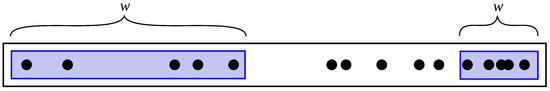
Figure 1.
Visualizing how to calculate R: The values are distributed for a subsample after being sorted from lowest to highest values. For illustration purposes, are the number of data points, there are 15 values, and . Note that only w spacing values on either extreme (minimum spacing on the left side) or (maximum spacing on the right side) are averaged over as the highlights show. The larger differences in small/large spacing implies greater density variation within a block.
Based on the operational definition for R (detailed in Equations (2)–(4), we note that . As the density variation within a block increases, R can only increase from 1, and a divergent density is indicated when . Furthermore, after consecutive sampled points are sorted in ascending order, the fluctuations that occur in their spacing causes R to increase away from 1 as the number of units increases. This latter trend will be true for any given statistical distribution, but we are specifically interested in discriminating density variations within a region that is typical of uniform density or slowly varying density (i.e., near uniform density), versus a region having large density variations. To quantify the distinction between low and high density variation requires developing a sample size dependent threshold. To establish a baseline for the threshold as a function of n, we apply the general statistical measure R to a uniform distribution, since random data cannot be expected to be more uniformly distributed than SURD.
To quantify the trend of how R increases as the number of units increases, we plot as a function of in Figure 2 for the case . It is interesting to observe that R exhibits a scaling law property as a function of number of units across a variety the distributions we considered. As expected, the uniform density case (SURD) yields the lowest . We find that the scaling law provides a good fit to SURD, with and , determined through least squares error linear regression. Notably, the parameters A and are rooted in fundamental statistical properties, which we demonstrate numerically. In other words, A and are not optimized hyperparameters that could depend on our selection of “training distributions”, while our approach holds universal appeal, it is important to acknowledge that w serves as a heuristic hyperparameter embedded in the operational definition of R, requiring optimization. We observe that for any fixed value of w we tested, R tends to approach a power law form in the limit . However, we aim to keep w small to enable the application of the divide and conquer procedure on small blocks, facilitating better treatment of singular densities.
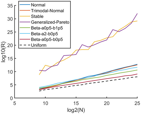
Figure 2.
Sample size dependence on statistical measure R: For the case that , it is seen that a simple power law describes how R scales as a function of n. These results are based on averaging over 100 realizations per n value. As expected, the uniform distribution (shown as a dashed black line) provides the lowest bound for R among all the distributions tested.
Fitting a scaling law to SURD for different window sizes, w, shows that provides robust and consistent results for individual realizations. Increasing w minimizes fluctuations in R across individual samples, but smaller w extends the power law to lower sample sizes and keeps computational cost to a minimum. Our heuristic analysis indicates that a value of is a suitable lower bound. Increasing w did not result in a significant improvement in accuracy beyond , while smaller values of w are viable, we select as it fulfills all necessary requirements, and decreasing w does not confer computational benefit.
To divide a block into two offspring, each containing subsamples of units from the parent block, there are two mechanisms of partitioning. The primary method partitions a block if for a given block under consideration, and the splitting process concludes once is achieved for all blocks. The secondary mechanism is used to further subdivide large blocks containing data points, where is determined primarily by hardware constraints. Importantly, all successive divisions of a parent block that satisfies the condition will also satisfy this condition for each of the children blocks having smaller subsamples. Therefore, when density variation does not cause a block division, the second mechanism will divide the block if it has more units than the predefined maximum, . This secondary partitioning rule ensures that a NMEM-worker will not require large memory needs. A practical cutoff of = 100,000 is employed.
NAPS achieves load balancing through block partitioning. To determine if the number of samples, n, within a block should be split in half, a “what-if” test is developed. First, we forecast the split and calculate R for the left and right blocks independently, denoted as and , respectively. The same equations for R are used, but we calculate the quantity for subsamples that have units (data points). Even when the density variation within these children subsamples are slightly greater than that for SURD, the test statistic will often remain less than because the sample size of each offspring is only half as much as the parent subsample. In this way, a self-similar threshold is created by using a shift in scale. As an alternative, we tried the formula , but this created more blocks and led to inferior results overall. Intuitively, represents the average density variation at the next level, which allows us to use the binary division rule given in Equation (1) to determine if a block should be split. As block sizes approach number of units, the blocks will stop splitting because they can no longer meet the criteria in Equation (1). This branching tree process is illustrated in Figure 3. In general the final tree that is generated can be unbalanced due to local divergent densities or heavy tails in other cases.
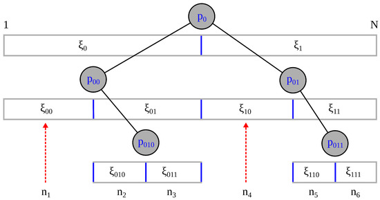
Figure 3.
Divide and conquer process: Partitions are generated from a sample of size N as the first partition, and then recursively divided into equal subsamples when the average density variation of offspring subsamples is above a maximum threshold. The final subsample sizes, , are shown at the final level of the unbalanced tree, with dashed red arrows pointing to distant partitions.
The divide and conquer process minimizes density variation within each subsample. This strategy leads to requiring a small number of Lagrange multipliers for accurate, smooth and fast estimates within all the partitions when using NMEM. Other methods such as local regression, spline fits, or KDE could be used to estimate the PDF within blocks. For example, the blocks with simple features are more suitable for simple KDE methods. In this work, when NAPS utilizes the NMEM method, which is a C++ code, the default settings are overridden by several modifiers. The normal default parameters are set for unknown input, but now, the blocks will have much less density variation that can be taken advantage of. For all internal blocks, (1) outlier detection is turned off; (2) maximum Lagrange multipliers are capped at 100; (3) smoothing level is increased to 100; (4) confidence level for the target score is relaxed from 70% to 20%, and (5) fixed boundary conditions are used by specifying the censor window. The leftmost block uses an open boundary condition on the left with a fixed boundary on the right, while the rightmost block uses open boundary conditions on the right with a fixed boundary on the left. The results are not sensitive to the exact values for these override settings. In addition, using the MATLAB implementation, KDE with reflective boundary conditions is applied to all blocks for PDF estimates. Section 3.5 provides a comparison of the results obtained when using KDE-workers and NMEM-workers to estimate PDFs within blocks.
2.2. Create Secondary Subsample Set
After establishing the subsample sizes representing layer 1 blocks, a secondary set of subsamples is created. The second set of subsamples, representing layer 2 blocks, overlap with the layer 1 blocks. To create a corresponding staggered layer 2 block, half of the points from its left layer 1 block are combined with half of the points from its right layer 1 block. This process is applied to all layer 2 blocks, each having two flanking layer 1 blocks. Therefore, there is one less layer 2 block than layer 1 blocks, and all layer 2 blocks are internal blocks. Figure 4a illustrates the collection of estimates for each of the blocks in both layers 1 and 2 for a trimodal distribution. This crude overlaying of independent PDF estimates in a staggered fashion provides a scaffold for the PDF. Since we have not noticed any difference in quality between the estimates in layer 1 compared to layer 2, we do not treat the estimates from either layer differently than the other layer. To ensure smoothness and continuity, the stitching method will be applied next.
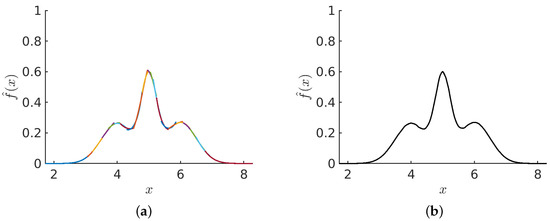
Figure 4.
Stitching process: (a) A set of independent PDF estimates for different subsamples for all blocks in both layers 1 and 2 are shown before stitching. This example considers a trimodel Gaussian mixture distribution of the form: (). (b) After the stitching process is applied to the collection of PDF estimates for all blocks, the resultant density estimate is shown.
2.3. Stitching Process
The stitching process involves two blocks taken from two different layers. At a particular point on the support for the , there will be two options to choose from, the PDF on the left, denoted as , or the PDF on the right, denoted as . The left and right blocks are uniquely determined by where the point of interest at x divides the block. The stitch makes no distinction as to which layer the block is a member of.
We define a variable u to monitor the linear proportion (i.e., fraction) of the probability contribution of a block relative to its right side. Operationally, let be an empirical cumulative distribution function (CDF) normalized such that u ranges from 0 to 1, where 0 and 1, respectively, represent the far most left and right sides of a block in terms of counting data points within it. Since every point in a block corresponds to a particular point on the x-axis, it is straightforward to construct two functions, called and , for the purpose to represent the fraction of density contribution from the left and right blocks at location . As such, with the exception of the first and last blocks, a stitch is made by averaging the two available left and right block estimates for the PDF in terms of weights given by their complementary CDF and CDF, respectively. However, the labeling of points by index k was done for conceptual purposes. We have estimates for any value of x as continuous functions. As such, we drop the index k, and understand that we can provide the value of the function at any x by interpolation. Note that there are data-driven nonlinear relations between x and and between x and .
Starting at and ending at , then for the left block will trace from to 1, while the right block will trace from 0 to . The interpolation is always in the mutually shared region where two estimates from and are available. The stitch formula is given as:
The PDF estimate becomes a weighted average of the two PDFs where the weight factors through the complementary CDF given by and the CDF given by are data-driven. Examples of the estimated CDF and complimentary CDF are shown in Figure 5a. It is seen that as the point of interest moves along the x-axis, the weight factors change in a continuous way in terms of and , which smooths out the two possible PDF estimates by a weighted mean given in Equation (5). A visual example of how the stitching process transforms the scaffold set of PDF estimates into a continuous function is given in Figure 5b where the end result is an interpolation between two estimated PDFs.
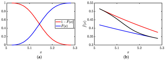
Figure 5.
Stitching process: (a) To facilitate a stitch, the estimated complementary CDF based on and the estimated CDF based on used in Equation (5) are shown as red and blue curves, respectively. (b) The resulting stitched density (black) as an interpolation between the left and right density estimates of a pair of blocks show as red and blue curves, respectively. This example is atypical as it shows the weighting from the left and right sides both range from 0 to 1. Typically the maximum values for the CDF and complimentary CDF are less than 1 over the mutually shared region of interest.
No stitch is performed for the far left and far right blocks, which use and , respectively. For internal blocks, the stitching procedure provides a smooth PDF estimate for all x as shown in Figure 4 that is piecewise differentiable across blocks.
2.4. NAPS Algorithm
The divide and conquer process using data-driven decisions based on the density variation characteristic, , to create a binary tree structure is called the optimal branching tree (OBT). Here, the pseudo code of NAPS is provided with implementation details, broken down into three algorithms, the first is to calculate .
Algorithm 1 splits a sample S in half, yielding samples and for the left and right sides. For each half, the statistical measure for density variation is calculated as and . This means that the differences, , are computed for and sorted, and then again for and sorted. For each set, and are calculated as the mean over the first and last w points of the sorted sets. In this way, and are calculated so that is returned.
Algorithm 2 initializes the sample size dependent threshold and partition set p for the sample or subsample S, with set size . The maximum number of levels allowed in the unbalanced binary tree is set to 40 for completeness, albeit not obtainable. The initial is computed, and b, the number of branches, is initialized to 1. The indexing on is based on tree level. If , the starting partition set is returned unchanged; otherwise, the block is partitioned into equal halves. The outer loop iterates over the number of levels in the tree, while the inner loop iterates through all branches currently under evaluation per tree level. The average of ratios for the left and right newly generated subsamples is stored in and evaluated against . If , the new partition is accepted; otherwise, the partition is rejected. After evaluating all branches for a given level, they are checked against . If and , the subroutine stops making any further levels of the tree and returns the set p. Otherwise, the algorithm updates the number of branches to evaluate and recursively continues.
The mathematical components of the stitching algorithm were described above. Algorithm 3 provides a pseudo code for the stitching process, and the complete NAPS algorithm is defined by the combination of Algorithms 1–3. Once all blocks are stitched together, there is one final step: normalizing the proposed PDF to 1. Additionally, different methods for estimating the PDF within a block, such as KDE, can be plugged into NAPS.
2.5. Test Distributions
Results for any density estimation comparison will inevitably vary from one distribution to the next. Specific features of a data sample may be more difficult for some methods to accurately estimate than others. NAPS has been tested against dozens of known distributions as well as mixtures of these distributions. For most of the results shown here, we have selected the following eight representative distributions: uniform on [0,1], normal (), trimodal Gaussian mixture model; (), Beta with three sets of parameters; , , , Stable and generalized Pareto . The specific features, challenges, and performance of each of these distributions will be discussed with examples in the next section. Based on reviewer suggestions, we also considered six additional distributions that include the generalized extreme value , i.e., GEV(2,2,2), Gumble, i.e., GEV(0,1,5), Fechet, i.e., GEV(1,1,5), Weibull , uniform mixture model; , and an equal weighted mixture modeling using a Cauchy, i.e., stable and a Beta distribution. These additional six distributions are very challenging and are discussed separately as a second test set in Section 3.
| Algorithm 1 algorithm |
|
| Algorithm 2 Optimized branching tree algorithm |
|
| Algorithm 3: Stitching method algorithm |
|
3. Results and Discussions
The results are presented in six subsections that consider different types of comparisons and assessment methods. The first three subsections provide an extensive comparison between NMEM and NAPS in terms of accuracy. Section 3.4 provides a detailed comparison of the computational efficiency of NMEM versus NAPS for both the serial version and the parallel computing version. In Section 3.5, a comparison is made between KDE, NMEM, NAPS(KDE), and NAPS(NMEM) in terms of both accuracy and computational efficiency. Finally, in Section 3.6, we show results for two specific challenging cases. We use NAPS without a qualifier to imply NAPS(NMEM), as it will be demonstrated that NAPS(NMEM) is the superior method in terms of trade-offs between accuracy and performance characteristics for a robust, fully automated high-throughput approach.
3.1. PDF Visual Comparison between NAPS and NMEM
Figure 6 displays visual examples of PDF estimates that highlight the differences between NMEM and NAPS for specific distributions and sample sizes. Recall that NMEM utilizes a random search method to estimate the Lagrange multipliers, meaning that different estimates can be produced upon multiple runs with the same sample data. Plotting multiple estimates provides a visual representation of the uncertainty, which decreases as the sample size increases. It is apparent that the variations in these estimates are due to random wiggles, as no common pattern is present across the different realizations.
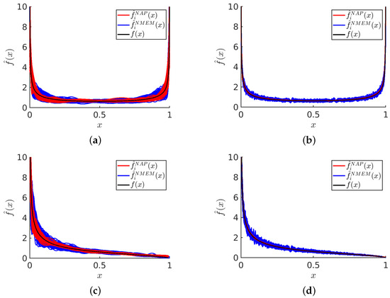
Figure 6.
Visualization of PDF estimates: For sample sizes of shown in panels (a,c) and shown in panels (b,d) a plot of 100 estimates visually compares how NAPS and NMEM handle divergent Beta distributions. Shown in panels (a,b) is the Beta(0.5, 0.5) distribution and (c,d) is the Beta(0.5, 1.5) distribution. The black line is used to show the theoretical distribution.
Despite the presence of random errors, each estimate is consistent with the data and statistical resolution, with the amplitude of the random error decreasing as the number of samples increases. This is true for both NMEM and NAPS; however, NAPS clearly has a smaller amplitude of random error. Although a smooth function is preferred, the source of these random wiggles derives from the generalized Fourier series employed by NMEM. The random wiggles that appear in NMEM can be greatly reduced by specifying a much higher smoothing level than the default value, but this risks removing sharp features in a PDF that are real. In general, the wiggles in the PDF can be influenced by both sharp features in the ground truth distribution and fluctuations in a sample.
The amplitude of random errors in NAPS is lower than in NMEM due to the small density variations typically found in individual data blocks when applying NMEM. This inherently reduces the need for a larger number of Lagrange multipliers and generates smoother estimates within each block. As density variation is minimized by the creation of these blocks, sharp features are rare within each block. Therefore, running NMEM at an elevated smoothing level within a block as a censor window is justified, incurring little risk of smoothing out a real sharp feature. Additionally, the stitching process smooths out edge mismatches, further contributing to generating smoother estimates with NAPS.
The PDF plots depicted in Figure 6 do not provide useful visualization of the tails of the distributions due to the scale used in the graphs. In Figure 7, we specifically focus on the tails of the distributions by presenting 100 independent data sets for samples and compare NAPS and NMEM estimates. Each plot shows the estimated complementary cumulative probability distribution function, , on a logarithmic scale to emphasize errors that occur in low-density tails. This allows us to visually gain a sense of the accuracy within the tails of four example distributions.
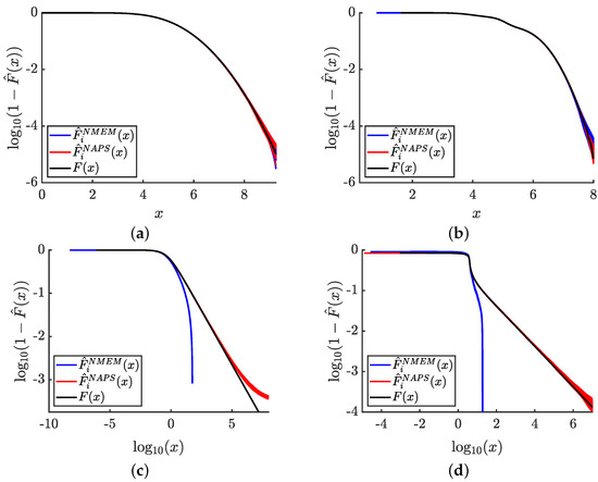
Figure 7.
Tail estimates: Complementary CDF estimates for 100 samples of size are shown for NAPS and NMEM for two rapidly decaying and two heavy tailed distributions. (a) normal(5, 1); (b) trimodal normal; (c) generalize-Pareto(2, 1, 0), and (d) stable(0.5, 0.05, 1, 4). The black line defines ground truth. Only the right side of the distributions is considered by focusing on , which allows to be plotted.
For the normal and trimodal normal distributions, respectively, shown in Figure 7a,b, it is observed that NAPS and NMEM exhibit similar degrees of high accuracy relatively deep into the rapidly falling tails. For the generalize-Pareto and stable distributions, respectively, shown in Figure 7c,d, NMEM fails to yield estimates deep into their tails due to its automated outlier detection, which can lead to excessive removal of “outliers” for distributions with extreme statistics. In such cases, preventing outlier removal by overriding the default setting can render it impossible for NMEM to fit the distribution at all. Therefore, outlier detection is a critical component for NMEM to function as a robust nonparametric probability density estimator.
In contrast, NAPS does not require outlier detection for internal blocks with fixed boundaries. Outlier detection is only necessary when there are one or two open boundaries. Consequently, NAPS can effectively estimate deep into the tails of a PDF, albeit with some error. The error in the tails arises because no attempt is made to model the asymptotic behavior of the heavy tails beyond the last empirical observation. As a result, normalization cannot be precisely defined without modeling the heavy tails asymptotically using an extrapolation process. Although it is possible to obtain good estimates of power law tails within the framework of NAPS using a semi-parametric version of NMEM on half-open blocks, such modeling goes beyond the scope of this work. Our semi-parametric modeling of heavy tails in an automated and adaptive way will be published elsewhere. Nevertheless, NAPS yields estimates with an accuracy commensurate with the statistical resolution set by the total number of samples, N, and offers a substantial advantage over NMEM.
3.2. Mean Percent Error Comparison between NAPS and NMEM
For each of the test distributions, we generated 100 independent data samples for sample sizes in increasing powers of two from to . PDF estimates, , were obtained for each data sample using NAPS and NMEM and compared to the ground truth, using mean percent error (MPE). The percent error (PE) for a given estimate at the value of x is defined as:
The empirical mean of PE over the entire range of the PDF for one sample is based on all units (sample points, N), given as:
Instead of using mean squared error (MSE), we calculated the MPE to compare the estimated and ground truth PDFs, which overcomes problems associated with disparate scales. In cases where the ground truth distribution has a singularity, it is possible for a small PE in regions where the density is extremely large be associated with an absolute error much larger than the absolute error within low-density regions with a large PE. As such, MSE is intrinsically biased toward high-density regions and cannot reflect how good an estimate is in low-density regions. Calculating PE across the entire PDF provides a reasonably fair comparison of error relative to the ground truth distributions. To avoid problems when the ground truth PDF is zero, the PE formula of Equation (6) has a minimum value for the denominator of . This minimum level decreases as the sample size increases to reflect statistical resolution. Using MPE to quantitatively evaluate accuracy has the added advantage of providing a good sense of error across disparate types of distributions.
Figure 8 presents box and whisker plots of MPE as a function of sample size across 100 tests for eight distributions. For the normal and uniform distributions shown in Figure 8a,b, respectively, the MPE values are comparable between the two estimators. However, NMEM does slightly better than NAPS for the normal distribution, which can be modeled exactly with only three Lagrange multipliers. This result is not surprising and is perhaps to be expected due to the similarity with performing a parametric fit. Although uniform can be exactly modeled with only one Lagrange multiplier, NAPS can still accurately estimate the distribution by splitting it into small blocks, each being relatively easy to identify as having uniform density. Unlike the normal distribution, which has distinct regions with disparate density (e.g., peak region versus half width and tails), NAPS applied to the uniform distribution must perform extra work to reconstruct the “obvious”. Thus, the normal and uniform are two special examples (requiring a specific low number of Lagrange multipliers) where decomposing a problem into many parts using divide and conquer increases overall difficulty in obtaining a smooth and accurate estimate.
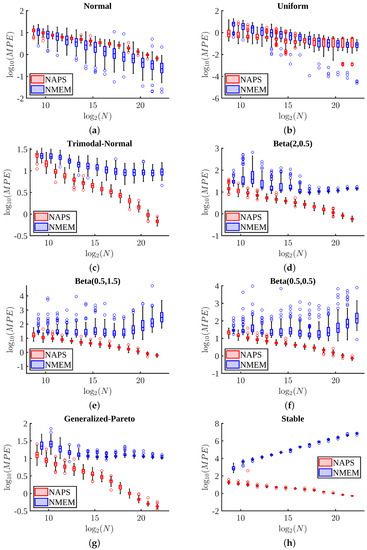
Figure 8.
Mean percent error comparisons: The MPE for the NAPS and NMEM estimators are compared using box and whisker plots for eight distributions and for sample sizes in the range – for 100 estimates per sample size for distributions: (a) normal(5, 1) (b) uniform(4, 8) (c) trimodal normal (d) Beta(2, 0.5) (e) Beta(0.5, 1.5) (f) Beta(0.5, 0.5) (g) generalized-Pareto(2, 1, 0) (h) and stable(0.5, 0.5, 1, 4). To avoid overlaps in data, NAPS and NMEM sample sizes are slightly displaced about the size being plotted.
For more challenging distributions, typically those containing sharp peaks, heavy tails, or divergences, as shown in Figure 8c–h, NAPS outperforms NMEM, particularly as the sample size increases. The advantage of breaking the large task into many smaller ones pays off in terms of accuracy in all of these cases. Moreover, NAPS generally shows an MPE of less than 35% at the smallest size of , except for the stable distribution, which starts with an MPE of 70%. However, there is a rapid improvement in accuracy in the form of a power-law as the sample size increases, based on visual inspection of the roughly straight lines for NAPS in all log-log graphs in Figure 8. In contrast, NMEM errors typically saturate or, in some cases, increase. It is worth noting that these levels of error in terms of MPE are also quite good compared to popular KDE methods since NMEM compares favorably to KDE (see Section 3.5 for direct comparisons involving KDE).
While the MPE plots in Figure 8 provide an overview of the average errors across the entire PDF estimate, we also consider where the greatest contribution to the MPE occurs over localized regions of a PDF. The plots in Figure 9 break down the MPE according to quantiles of the CDF for the stable distribution, as demonstrated in Figure 9a. Note that the only modification to the way MPE is calculated is to include all data points in the averaging procedure shown in Equation (7) that are members of the specified quantile range, which we consider in 2% increments. The remaining plots in this figure compare NAPS and NMEM for increasing sample sizes, with several key observations. In general, errors decrease for larger sample sizes with NAPS but remain roughly constant for NMEM, consistent with Figure 8h. Figure 9b–d show that the improvement in MPE with sample size for NAPS is primarily driven by the low-density tails. This point will be further highlighted with examples in the next section.
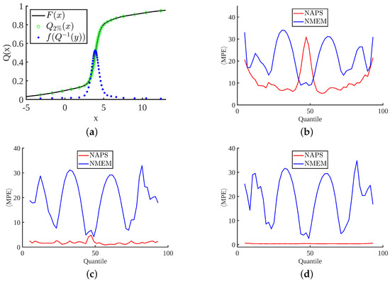
Figure 9.
Localizing percent error within quantiles: (a) Displays the CDF, 2% quantiles, and PDF for the stable distribution evaluated at the quantiles. The mean percent error (MPE) is plotted per quantile for samples sizes: (b) (c) (d) .
3.3. SQR Comparison between NAPS and NMEM
An additional method for determining the quality of an estimate is the scaled quantile residual (SQR) for measuring uncertainty, defined as,
where k refers to the position index ranging from 1 to the sample size N, , and for each data sample point . The square root term scales the residuals by the sample size N, which leads to a sample size invariant measure. When plotting the SQR as a function of position k, it has been demonstrated [24,25,26,31] that the expected values will fall within an oval shaped region as defined by the dotted lines shown in Figure 10. The inner dashed lines represent the area where 50% of residuals are expected to fall, and the outer lines represent the 98th percentile. Therefore, when calculating the SQR for a CDF estimated from a sample , these plots are an effective visualization tool for diagnosing where estimates may fall outside of expected ranges.

Figure 10.
Scaled quantile residual comparisons: The SQR calculations for single estimates from a Beta(2, 0.5) distribution for (a) NAPS for . (b) NMEM for . (c) NAPS for . (d) NMEM for .
In Figure 10, all SQR values that fall outside of the 98th percentile are colored in red. Statistically, we would expect approximately 2% of these points to appear outside of the large oval. However, significant deviations from this expectation, particularly if the errors are periodically spaced, is an indication that the estimate is poorly fitted to the data in this region. All the SQR plots show in Figure 10 are for estimates of the Beta (2, 0.5) distribution, which has very low density on the left and a divergence in density on the right. Plots in the (first, second) columns are for (NAPS, NMEM) shown for samples sizes of (, ) for the (top, bottom) rows. As with other examples shown thus far, the divergence is difficult to fit properly for NMEM with increasing sample size, as indicated by the outliers colored in red. The oscillations, such as those in Figure 10d, tend to increase in both amplitude and frequency, which often corresponds to unnatural wiggles, whereas the lower amplitude oscillations in the NAPS plots for Figure 10a,c indicate a smoother PDF.
3.4. Computation Time
To evaluate the computational efficiency of NAPS and NMEM, we measured the total computation times for all eight distributions at sample sizes ranging from to . On our hardware, our current C++ NMEM implementation can reliably provide estimates up to for a wide range of distributions with default settings, although the quality of estimate can deteriorate for difficult cases. For the NAPS implementation, we consider two cases: serial using a single processor and parallel using 40 processors. In the parallel processing case, we extend the largest sample size by more than an order of magnitude to , but this size does not reflect hardware or implementation limits. However, for the series case using a single processor, memory limitations sets a sample size limit to .
Figure 11a shows the wall time (total elapsed time) averaged over 100 trials for sample sizes up to for both methods, and 10 trials for to for NAPS (serial). The times are also averaged over all eight distributions, with error bars indicating the variation across distributions. The variation in NMEM is noticeably larger than NAPS, especially for large sample sizes. This is expected because, by separating the data into more uniform density blocks, the wall time in NAPS is dictated more by the number of blocks than the details of the original distribution. As predicted, the time to compute all the blocks in NAPS, even when run in serial, is typically less than processing all the data together with NMEM. These times include the overhead of separating the blocks and stitching the estimates together.
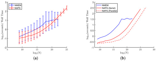
Figure 11.
Computational times: The mean wall time of the NMEM and NAPS estimators as a function of sample size: (a) serial runs for NMEM and NAPS with error bars for variations across distributions with a single processor (b) includes a dashed line for parallel runs with 40 processors.
Figure 11b displays a dashed line representing the average wall time across 10 trials and the eight distributions for NAPS run with 40 processors. The NMEM and NAPS (serial) data shown in Figure 11a is re-shown, but without the error bars for clarity. Note that the results are identical for NAPS serial versus parallel with the same seed for the random number generator. The NMEM wall time begins to level off around a sample size of , primarily due to the more challenging distributions that NMEM struggles to estimate effectively. NMEM has safeguards implemented that will abort its random search procedure to optimize Lagrange multipliers when it becomes clear that progress towards an improved estimate is not being made at a sufficiently fast rate.
While the hardware limit on memory when running NAPS in serial is larger than the limit of NMEM as a one-shot method since block sizes are smaller, the information for all blocks still needs to be stored. This results in a modest increase in the memory limit for NAPS (serial). This practical hardware limitation is further increased when the blocks are distributed among multiple processors, resulting in significant time savings and the ability to increase the sample size. Here, we show results up to sample sizes of . This is not due to a hardware limit on the sample size but rather a practical limit in available computing resources. Additional processors and memory would allow for substantial increases in sample size beyond . Ongoing work includes the optimization of data structures combined with parallel computing implementations in C++ for a future update release on our user-friendly software in C++, R and MATLAB, and a first Python version. These software updates will include hardware aware modes of operations.
3.5. KDE, NMEM, NAPS(KDE) and NAPS(NMEM) Comparisons
In this subsection, we explore the use of KDE as an alternative to NMEM for obtaining density estimations within blocks. To differentiate between the KDE and NMEM base methods within NAPS, we will refer to them as NAPS(KDE) and NAPS(NMEM), respectively. Figure 12 compares typical results based on one data sample using KDE, NMEM, NAPS(KDE), and NAPS(NMEM). This figure clearly shows that without careful adjustments and attention from a highly trained domain expert with knowledge of the input data characteristics, KDE can be substantially wrong.
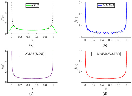
Figure 12.
Comparison of four density estimate methods: For a Beta(0.5, 0.5) sample of size . (a) MATLAB standard ksdensity() function; (b) NMEM; (c) NAPS using ksdensity() with reflective boundaries for estimating block densities, and (d) NAPS using NMEM for estimating block densities.
The other three methods (NMEM or NAPS using KDE or NMEM) can be used to provide an automated process for high throughput applications where no prior knowledge of the input data characteristics is expected or needed. Although NMEM produces an accurate and quite reasonable estimate, as shown in Figure 12b, it is not sufficiently smooth. This example visually suggests that NAPS provides accurate and smooth estimates robustly, regardless of whether the base estimator used in blocks is KDE or NMEM. This result also demonstrates that the partitioning method is key to success, so that each block provides enough support to make a density prediction that is relatively smooth with no sharp features. It is worth noting that one can construct a data sample to break any of these methods. However, using the SQR measure, a flag will result when the estimation is likely not correct. In the four cases shown in Figure 12, only the KDE method will be flagged.
Figure 13 shows the results for the same Beta-distribution used in Figure 12 for the KDE, NMEM, NAPS(KDE), and NAPS(NMEM) methods. However, for all the plots in Figure 13, we consider 20 different samples of size . It is clear that the KDE method is easily flagged in Figure 13a as a failed estimate. Interestingly, the SQR plots shown in Figure 13b,d for the NMEM and NAPS(NMEM) methods fall largely within the 98th percentile. Importantly, both of these SQR plots appear similar to what would be expected of SQR plots for SURD. At a qualitative level, for this example distribution, the SQR plots from NAPS(NMEM) visually resemble SQR plots for SURD slightly better. In contrast, the good SURD-like characteristics in SQR plots do not appear for the NAPS(KDE) case. For NAPS(KDE), Figure 13c shows the SQR traces are unnaturally concentrated near the center, there is a systematic linear trend line that indicates over-fitting, and for some of the estimates, the SQR plot exceeds the 98th percentile to a sufficient degree that this estimate would be flagged as a failed estimate. However, unless the SURD pattern in SURD is quantified, the systematic error found in all the NAPS(KDE) estimates (e.g., a linear line) could go undetected. This single example suggests it is best to use NAPS(NMEM) for robust and accurate results.
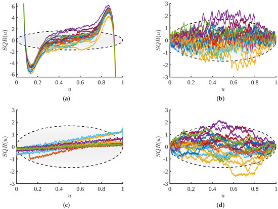
Figure 13.
Scaled quantile residual comparisons: The SQR plots are shown for 20 estimates for a Beta(0.5, 0.5) distribution using a sample size of and four distinct methods. (a) KDE; (b) NMEM; (c) NAPS(KDE), and (d) NAPS(NMEM).
We compare the overall accuracy in the PDF estimations from NAPS(KDE) and NAPS(NMEM) using the MPE measure in Figure 14. Across all eight distributions considered in test set 1 with sample sizes ranging from to , it is evident that NAPS(NMEM) consistently provides superior accuracy over NAPS(KDE). Interestingly, for the heavy-tailed generalized Pareto and stable distributions (as shown in Figure 14g,h), it is observed that NAPS(NMEM) has the least advantage over NAPS(KDE) for all sample sizes.
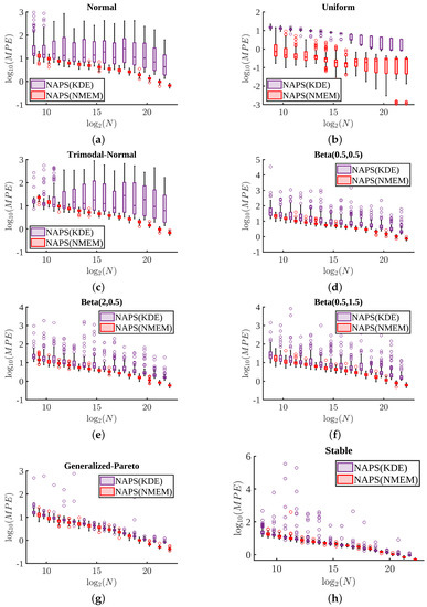
Figure 14.
Mean percent error comparisons: Following Figure 8, the MPE for the NAPS(KDE) and NAPS(NMEM) estimators are compared using box and whisker plots for 100 trials: (a) normal(5, 1) (b) uniform(4, 8) (c) trimodal normal (d) Beta(2, 0.5) (e) Beta(0.5, 1.5) (f) Beta(0.5, 0.5) (g) generalized-Pareto(2, 1, 0) (h) and stable(0.5, 0.5, 1, 4). To avoid overlaps in data, NAPS(KDE) and NAPS(NMEM) sample sizes are slightly displaced about the size being plotted.
The MPE accuracy from NMEM, NAPS(KDE) and NAPS(NMEM) are listed in Table 1 for all fourteen distributions considered in test sets 1 and 2 for three sample sizes. Sometimes NMEM does better than NAPS(KDE) and vice versa. We devise a relative error ratio (RER) that divides the MPE of NAPS(NMEM) by the minimum MPE between NMEM and NAPS(KDE). Almost always RER is less than 1, indicating NAPS(NMEM) is overall the best method. Nevertheless, there are a few cases where RER is greater than 1. This can occur when the minimum error from NMEM or NAPS(KDE) is very low. In these cases, the overall accuracy of NAPS(NMEM) can be very good, despite having RER > 1.

Table 1.
The mean and standard deviations of MPE for 100 realizations for all 14 distributions considered at three different sample sizes for the NMEM, NAPS(KDE) and NAPS(NMEM) density estimation methods, and RER as a comparison measure. The bold RER values indicate that although RER > 1, NAPS(NMEM) remains very accurate. The RER values greater than 100 have an asterisk to indicate that NAPS(NMEM) introduced more error in the density estimate than it removed.
These results suggest that NAPS(NMEM) is generally the most accurate method. Yet Figure 8 shows that for the normal distribution (and possibly other simple distributions), NMEM has greater accuracy than NAPS(NMEM). This occurs because a Gaussian distribution requires three Lagrange multipliers. This global knowledge is lost when the data is split up into small blocks. Special circumstances puts NAPS(NMEM) at a disadvantage. However, for a robust estimator that is fully automatic and will not require prior knowledge of the sample distribution, NAPS(NMEM) provides the most consistent high accuracy estimates across diverse distributions, and an extensive range of sample sizes.
Figure 15 compares the computational times for KDE, NAPS(KDE), and NAPS(NMEM). As expected, KDE is much faster than NAPS. Nevertheless, NAPS(KDE) is slower than NAPS(NMEM) for sample sizes above because block partitioning corroborates with properties that are favorable for NMEM. That is, NMEM ensures reasonable load balance by using a low number of Lagrange multipliers to model the PDF in each block. Since the computational time for KDE depends only on the number of sample points within a block, NAPS(KDE) is faster than NAPS(NMEM) for sample sizes less than due to the initialization overhead cost of NMEM. However, since a large fraction of the total computational cost comes from partitioning the blocks, which is independent of the density estimation method, NAPS(KDE) and NAPS(NMEM) have similar computational speeds. Taking into account accuracy-speed tradeoffs, NAPS(NMEM) has the best performance. Furthermore, ongoing work on the C++ NAPS(NMEM) implementation suggests a significant gain in speed can be achieved.
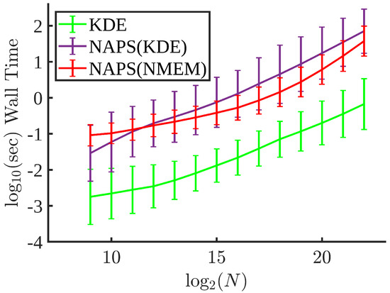
Figure 15.
Computational times: The mean wall time for 100 trials of KDE, NAPS(KDE) and NAPS(NMEM) with error bars for the same eight distributions used everywhere else as a function of sample size. Wall times are computed for the parallel runs using 40 processors.
3.6. Illustration of Two Bad Cases
The PDF estimates obtained for sample sizes of and using KDE, NMEM, NAPS(KDE), and NAPS(NMEM) are presented in Figure 16 and Figure 17 for the Cauchy-Beta mixture model and the uniform mixture model, respectively. The assumption that reducing block size will result in smoother estimates proves invalid in these cases. The presence of sharp features within certain blocks poses an inherent challenge, leading to the Gibbs phenomenon associated with Fourier series approximations of sharp discontinuities. Addressing these pathological cases necessitates the abandonment of the smoothness assumption, which will be addressed through self-detection of edge effects in future work. Nonetheless, the NAPS density estimate captures the discontinuity well while providing a reasonably accurate estimate everywhere else. These results warrant further discussion.
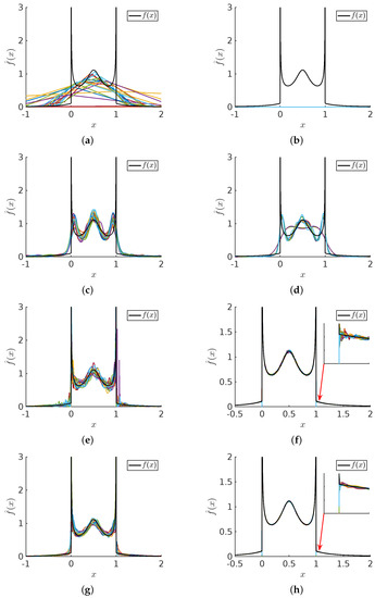
Figure 16.
Cauchy-Beta distribution comparisons: For sample sizes (left column) and (right column) 20 trials are shown for (a,b) KDE (c,d) NMEM (e,f) NAPS(KDE) (g,h) NAPS(NMEM). The black line shows the ground truth.
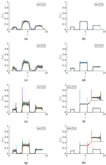
Figure 17.
Uniform mixture model comparisons: For sample sizes (left column) and (right column) 20 trials are shown for (a,b) KDE (c,d) NMEM (e,f) NAPS(KDE) (g,h) NAPS(NMEM). The black line shows the ground truth.
In Figure 16, the simple KDE method performs poorly for a sample size of and fails completely with a sample size of . Surprisingly, the one-shot NMEM method exhibits good performance for these sample sizes but fails to capture all the intricate features due to the requirement of hundreds of Lagrange multipliers. NAPS(KDE) resolves these issues, providing highly accurate results without employing a Fourier series approach. However, it exhibits an artifact resembling the Gibbs phenomenon at the discontinuities. NAPS(NMEM) yields the most visually appealing estimate despite displaying the Gibbs phenomenon at the edges. Magnified regions around the discontinuities provide a detailed view of the Gibbs phenomenon. Although challenging to eliminate, these artifacts are comprehensible and manageable.
In Figure 17, all methods perform reasonably well for the uniform mixture model. Similar to the Cauchy-Beta mixture model, the step discontinuities pose analogous challenges. Without the singularities, the basic KDE works, although it over-smooths the discontinuities as an intrinsic disadvantage. For this problem, even using a sample size of , KDE over smooths the sharp step characteristics including the discontinuities at the far left and far right boundaries. The SQR test would clearly reject this solution as viable. Notice that NAPS(KDE) virtually eliminates this over-smoothing problem of KDE, but then it has an apparent Gibbs phenomena at the discontinuities. We see that the NAPS(NMEM) method effectively captures the uniform mixture model, despite errors caused by local Gibbs phenomena at the sharp internal edges.
It is worth emphasizing that the cases presented here represent the worst scenarios in terms of the global MPE, as indicated in Table 1. However, visually, the error does not appear to be significantly high, despite the elevated RER. This discrepancy arises because, as overall accuracy improves, a better estimate can be obtained closer to a discontinuity or singularity. Since a singularity or a discontinuity cannot be accurately modeled in either the Fourier or smoothing kernel frameworks, the majority contribution to the MPE arises from the density estimate near such points. Fortunately, these localized issues can be easily addressed using the divide and conquer approach. In this regard, NAPS(KDE) not only improves upon KDE but also provides a means to automate bandwidth selection. Nevertheless, when considering the data as a whole, it becomes evident that NAPS(NMEM) emerges as the clear winner in terms of overall accuracy and computational efficiency.
4. Conclusions
The NAPS algorithm has been demonstrated to be an effective divide and conquer approach to density estimation across a diverse set of fourteen distributions, ranging in difficulty from easy to very challenging. The challenging distributions include discontinuities or singularities, many examples of heavy tails and a mixture model that combines a Beta distribution having two singularities with a Cauchy distribution. We considered sample sizes ranging from to . A key aspect of NAPS is the development of a novel statistical measure, denoted by R, that quantifies the density variation within a given subsample of data, referred to as a block. Specifically, R is the ratio of the greatest spacing in data points to the lowest spacing within a block. We found that R scales as a power law for all distributions we checked. This general R statistic has proven to be a useful scale invariant decision trigger for effective data partitioning in terms of relative density variation within a block. To our knowledge this useful R statistical measure has not been previously investigated in the statistics literature.
The NAPS method can use different density estimation methods for estimating density within blocks of data that define partitioned subsamples. A data-driven stitching method is defined to develop a smooth overall continuous PDF estimate. Accuracy was quantified in two ways: through percent error between the estimated density and the ground truth PDF, and through the scaled quantile residual (SQR). We find that the estimates using NAPS(NMEM) produced a SQR that looked almost indistinguishable from that of sampled uniform random data (SURD) as it should. Although NAPS(KDE) has many advantages over KDE, such as adaptive bandwidth and handling boundaries better, it was noted that its SQR deviated from the expected characteristics of SURD. It is found that employing NMEM as the base method applied to all blocks is the most effective in both accuracy and speed. The NAPS(NMEM) approach extends the capabilities of NMEM to a larger class of distribution types and improves the ability to accurately estimate the underlying data with no a priori knowledge from the user. Furthermore, the estimates from NAPS are visibly smoother and calculated much more efficiently than NMEM. By focusing on partitioning a sample into more manageable subsamples using NMEM-workers in parallel computing, NAPS can efficiently handle large samples with over one hundred million units.
In conclusion, the NAPS algorithm represents a novel approach to obtain accurate density estimation, serving as an appropriate tool for fully automated high throughput applications. Future improvements are being developed in regards to treating the left and right blocks differently within the framework of NMEM to include semi-parametric modeling of heavy tails. Ongoing work also involves incorporating NAPS demonstrated here using MATLAB into our C++ code, and integrate this technical advance into multiple existing software as updates in C++, R, MATLAB, and to provide a Python version as well.
Supplementary Materials
The following are available at https://www.mdpi.com/article/10.3390/a16070310/s1: MATLAB scripts for data generation and post processing.
Author Contributions
Conceptualization, D.J.J. and Z.D.M.; methodology, J.F., Z.D.M. and D.J.J.; software, Z.D.M.; validation, Z.D.M. and J.F.; formal analysis, D.J.J.; investigation, Z.D.M. and J.F.; resources, D.J.J.; data curation, Z.D.M.; writing—original draft preparation, Z.D.M.; writing—review and editing, J.F. and D.J.J.; visualization, Z.D.M. and J.F.; supervision, D.J.J.; project administration, D.J.J. All authors have read and agreed to the published version of the manuscript.
Funding
This research received no external funding.
Data Availability Statement
All code that was used to generate the data and perform the calculations and analysis of the data are given in Supplementary Materials.
Acknowledgments
The computing resources and support used to produce the results presented in this paper were provided by the University Research Computing group in the Office of OneIT at the University of North Carolina at Charlotte. We also like to thank Michael Grabchak for useful discussions during the early stages of this project.
Conflicts of Interest
The authors declare no conflict of interest.
Abbreviations
The following abbreviations are used in this manuscript:
| Probability Density Function | |
| CDF | Cumulative Density Function |
| SQR | Scaled Quantile Residual |
| SURD | Sampled Uniform Random Data |
| KDE | Kernel Density Estimation |
| NMEM | Nonparametric Maximum Entropy Method |
| NAPS | Nonparametric Adaptive Partitioning and Stitching |
| OBT | Optimal Branching Tree |
| MPE | Mean Percent Error |
| PE | Percent Error |
References
- Rosenblatt, M. Remarks on Some Nonparametric Estimates of a Density Function. Ann. Math. Stat. 1956, 27, 832–837. [Google Scholar] [CrossRef]
- Whittle, P. On the Smoothing of Probability Density Functions. J. R. Stat. Soc. Ser. B Methodol. 1958, 20, 334–343. [Google Scholar] [CrossRef]
- Parzen, E. On Estimation of a Probability Density Function and Mode. Ann. Math. Stat. 1962, 33, 1065–1076. [Google Scholar] [CrossRef]
- Silverman, B.W. Density Estimation for Statistics and Data Analysis; Monographs on Statistics and Applied Probability; Chapman and Hall: London, UK, 1986; Includes Bibliographical References; pp. 59–165. [Google Scholar]
- Wand, M.P.; Jones, M.C. Kernel Smoothing, 1st ed.; Monographs on Statistics and Applied Probability; Chapman & Hall: London, UK; New York, NY, USA, 1995; p. xii. 212p. [Google Scholar]
- Chiu, S.T. A Comparative Review of Bandwidth Selection for Kernel Density Estimation. Stat. Sin. 1996, 6, 129–145. [Google Scholar]
- Abramson, I.S. Adaptive Density Flattening–A Metric Distortion Principle for Combating Bias in Nearest Neighbor Methods. Ann. Stat. 1984, 12, 880–886. [Google Scholar] [CrossRef]
- Borrajo, M.I.; González-Manteiga, W.; Martínez-Miranda, M.D. Bandwidth selection for kernel density estimation with length-biased data. J. Nonparametric Stat. 2017, 29, 636–668. [Google Scholar] [CrossRef]
- Breiman, L.; Meisel, W.; Purcell, E. Variable Kernel Estimates of Multivariate Densities. Technometrics 1977, 19, 135–144. [Google Scholar] [CrossRef]
- Gallego, J.A.; Osorio, J.F.; González, F.A. Fast Kernel Density Estimation with Density Matrices and Random Fourier Features; Springer: Cham, Switzerland, 2022. [Google Scholar] [CrossRef]
- Sheather, S.J. Density Estimation. Stat. Sci. 2004, 19, 588–597. [Google Scholar] [CrossRef]
- Chandra, O. Choice of the Bandwidth in Kernel Density Estimation. Int. J. Sci. Res. (IJSR) 2020, 9, 750–754. [Google Scholar]
- Florence, K.; Leonard, K.A. Efficiency of various Bandwidth Selection Methods across Different Kernels. IOSR J. Math. (IOSR-JM) 2019, 15, 55–62. [Google Scholar]
- Saito, K.; Yano, M.; Hino, H.; Shoji, T.; Asahara, A.; Morita, H.; Mitsumata, C.; Kohlbrecher, J.; Ono, K. Accelerating small-angle scattering experiments on anisotropic samples using kernel density estimation. Sci. Rep. 2019, 9, 1526. [Google Scholar] [CrossRef]
- Saule, E.; Panchananam, D.; Hohl, A.; Tang, W.; Delmelle, E. Parallel Space-Time Kernel Density Estimation. In Proceedings of the 2017 46th International Conference on Parallel Processing (ICPP), Bristol, UK, 14–17 August 2017; pp. 483–492. [Google Scholar] [CrossRef]
- Lin, Y.S.; Heathcote, A.; Holmes, W.R. Parallel probability density approximation. Behav. Res. Methods 2019, 51, 2777–2799. [Google Scholar] [CrossRef] [PubMed]
- Lopez-Novoa, U.; Sáenz, J.; Mendiburu, A.; Miguel-Alonso, J. An efficient implementation of kernel density estimation for multi-core and many-core architectures. Int. J. High Perform. Comput. Appl. 2015, 29, 331–347. [Google Scholar] [CrossRef]
- Monteiro, A.M.; Santos, A.A.F. Parallel computing in finance for estimating risk-neutral densities through option prices. J. Parallel Distrib. Comput. 2023, 173, 61–69. [Google Scholar] [CrossRef]
- Mitchell, R.; Frank, E.; Holmes, G. An Empirical Study of Moment Estimators for Quantile Approximation. ACM Trans. Database Syst. 2021, 46, 1–21. [Google Scholar] [CrossRef]
- Tanaka, H.; Takata, M.; Nishibori, E.; Kato, K.; Iishi, T.; Sakata, M. ENIGMA: Maximum-entropy method program package for huge systems. J. Appl. Crystallogr. 2002, 35, 282–286. [Google Scholar] [CrossRef]
- Michailidis, P.D.; Margaritis, K.G. Parallel Computing of Kernel Density Estimation with Different Multi-core Programming Models. In Proceedings of the 2013 21st Euromicro International Conference on Parallel, Distributed, and Network-Based Processing, Belfast, UK, 27 February–1 March 2013; IEEE: Piscataway, NJ, USA, 2013; pp. 77–85. [Google Scholar] [CrossRef]
- Racine, J. Parallel distributed kernel estimation. Comput. Stat. Data Anal. 2002, 40, 293–302. [Google Scholar] [CrossRef]
- Majdara, A.; Nooshabadi, S. Efficient Density Estimation for High-Dimensional Data. IEEE Access 2022, 10, 16592–16608. [Google Scholar] [CrossRef]
- Farmer, J.; Jacobs, D. High throughput nonparametric probability density estimation. (Research Article) (Report). PLoS ONE 2018, 13, e0196937. [Google Scholar] [CrossRef]
- Farmer, J.; Jacobs, D.J. MATLAB tool for probability density assessment and nonparametric estimation. SoftwareX 2022, 18, 101017. [Google Scholar] [CrossRef]
- Farmer, J.; Jacobs, D. The R Journal: PDFEstimator: An R Package for Density Estimation and Analysis. R J. 2022, 14, 305–319. [Google Scholar] [CrossRef]
- Donoho, D.L.; Johnstone, I.M.; Hoch, J.C.; Stern, A.S. Maximum Entropy and the Nearly Black Object. J. R. Stat. Soc. Ser. B Methodol. 1992, 54, 41–81. [Google Scholar] [CrossRef]
- Chen, S.; Rosenfeld, R. A survey of smoothing techniques for ME models. IEEE Trans. Speech Audio Process. 2000, 8, 37–50. [Google Scholar] [CrossRef]
- Dudík, M.; Phillips, S.J.; Schapire, R.E. Maximum Entropy Density Estimation with Generalized Regularization and an Application to Species Distribution Modeling. J. Mach. Learn. Res. 2007, 8, 1217–1260. [Google Scholar]
- Armstrong, N.; Sutton, G.J.; Hibbert, D.B. Estimating probability density functions using a combined maximum entropy moments and Bayesian method. Theory and numerical examples. Metrologia 2019, 56, 15019. [Google Scholar] [CrossRef]
- Farmer, J.; Merino, Z.; Gray, A.; Jacobs, D. Universal Sample Size Invariant Measures for Uncertainty Quantification in Density Estimation. Entropy 2019, 21, 1120. [Google Scholar] [CrossRef]
- Farmer, J.; Allen, E.; Jacobs, D.J. Quasar Identification Using Multivariate Probability Density Estimated from Nonparametric Conditional Probabilities. Mathematics 2023, 11, 155. [Google Scholar] [CrossRef]
Disclaimer/Publisher’s Note: The statements, opinions and data contained in all publications are solely those of the individual author(s) and contributor(s) and not of MDPI and/or the editor(s). MDPI and/or the editor(s) disclaim responsibility for any injury to people or property resulting from any ideas, methods, instructions or products referred to in the content. |
© 2023 by the authors. Licensee MDPI, Basel, Switzerland. This article is an open access article distributed under the terms and conditions of the Creative Commons Attribution (CC BY) license (https://creativecommons.org/licenses/by/4.0/).