Quantifying Uncertainties in OC-SMART Ocean Color Retrievals: A Bayesian Inversion Algorithm

Abstract

The Ocean Color—Simultaneous Marine and Aerosol Retrieval Tool (OC-SMART) is a robust data processing platform utilizing scientific machine learning (SciML) in conjunction with comprehensive radiative transfer computations to provide accurate remote sensing reflectances ($R_{\mathrm{rs}}$ estimates), aerosol optical depths, and inherent optical properties. This paper expands the capability of OC-SMART by quantifying uncertainties in ocean color retrievals. Bayesian inversion is used to relate measured top of atmosphere radiances and a priori data to estimate posterior probability density functions and associated uncertainties. A framework of the methodology and implementation strategy is presented and uncertainty estimates for $R_{\mathrm{rs}}$ retrievals are provided to demonstrate the approach by applying it to MODIS, OLCI Sentinel-3, and VIIRS sensor data.

1. Introduction

Remote sensing of the ocean is now routinely performed by using instruments deployed on satellite platforms [1,2] to measure the radiance emerging at the top of the atmosphere and then apply an atmospheric correction (AC) algorithm [3] to remove all but the water-leaving radiance component [4] or the closely related remote sensing reflectance ($R_{\mathrm{rs}}$). From the $R_{\mathrm{rs}}$ determined in the AC step, various ocean color products can be inferred, such as chlorophyll-a concentration [5], suspended particle matter [6], turbidity, and phytoplankton abundance [7]. Water quality is crucial to life in nearby regions [8,9], so it is of the utmost importance that measurement data with low bias and low uncertainty can be obtained. The uncertainty associated with a measurement characterizes the dispersion of the values that could reasonably be attributed to the property being measured [10,11,12]. In this paper, the metric used to express uncertainty associated with a measurement will be the standard deviation.

Several AC algorithms have have been developed to estimate the water-leaving radiance and achieved reasonable results in open ocean areas where the water-leaving radiances at near-infrared (NIR) wavelengths are negligible. Significant issues remain however; in coastal waters, which are not black in the NIR, negative water-leaving radiances are frequently produced by traditional AC algorithms [13,14]. In addition, aerosols in coastal areas often dramatically differ from those encountered over the open ocean, so any realistic AC approach should take into account the diversity of atmospheric and oceanic conditions encountered in such complex environments. Turbid waters, whitecaps, and sunglint can also lead to unreliable results. Various attempts to improve AC algorithms have been proposed, such as (i) using a turbid water flag to switch between correction algorithms depending on the region [15], (ii) changing the bio-optical model in an iterative manner [16], (iii) determining atmosphere–ocean properties simultaneously [17], (iv) employing a multi-band approach [18], (v) incorporating hyperspectral data [19], (vi) optimizing for sunglint through the use of a polynomial function [20], and (vii) using a coupled ocean/atmosphere inversion scheme based on neural networks [21]. AC algorithms that produce the highest quality results often use several of these improvements in conjunction to form a more complete model of the ocean and atmosphere.

Traditional AC approaches typically do not provide uncertainty estimates, which should be included, however, to gain confidence in retrieved results. Recently, some studies have discussed uncertainty issues based on optimal estimation (Bayesian inversion) [22,23,24]. Algorithms based on neural networks, such as C2RCC [25] and SWARM [26], provide uncertainties based on a comparison of radiative transfer model simulations and IOP inversions of the training datasets. These uncertainties reflect the difference between estimated ocean color retrievals and training simulations. Another approach is to use an ensemble of neural networks [27] with differing initializations to perform spectral inversion. These approaches for quantifying retrieval uncertainty rely heavily on the capability of algorithms to produce good match-ups between simulations and training data, as poor match-ups will lead to larger uncertainties. In two recent papers [28,29], the authors discuss steps to quantify pixel-level uncertainties using a derivative approach to propagate uncertainties through the $R_{\mathrm{rs}}$ retrieval process, primarily focusing on uncertainties arising from atmospheric correction. This approach allows one to account for uncertainties from a wide range of sources, but, in practice, not all source uncertainty information is available and several estimates and assumptions about the system need to be made.

The Ocean Color—Simultaneous Marine and Aerosol Retrieval Tool (OC-SMART) approach utilizes scientific machine learning (SciML) in conjunction with radiative transfer computations of the coupled atmosphere–water system to perform the AC step and retrieve water products from the resulting $R_{\mathrm{rs}}$ estimates [14]. The OC-SMART data processing platform employs a radiative transfer model for the coupled atmosphere–water system, AccuRT [30], that accounts for a variety of atmospheric and oceanic conditions likely to be encountered in nature. The OC-SMART approach resolves the negative water-leaving radiance problem, and is used to retrieve aerosol optical depths and remote sensing reflectances ($R_{\mathrm{rs}}$) as a function of wavelength on a pixel by pixel basis. These $R_{\mathrm{rs}}$ estimates are then used to infer inherent optical properties (IOPs), including absorption coefficients due to phytoplankton, detritus, and Gelbstoff, and backscattering coefficients due to particulates. However, these retrieved IOPs do not contain uncertainty estimates at present. To address this shortcoming, in this paper we focus on how to quantify uncertainties in retrieval parameters produced by OC-SMART. Since the accuracy of the remote sensing reflectance $R_{\mathrm{rs}}$ is critical to obtain high-quality water IOPs, our main target in this paper is to determine $R_{\mathrm{rs}}$ uncertainties associated with errors in measurements and a priori information. We chose to focus on a Bayesian inversion approach because of its ability to estimate uncertainties on a pixel by pixel basis and its flexibility to being updated if and when new a priori and/or measurement error information becomes available.

Section 2 presents an overview of OC-SMART in regards to its methods, advantages compared to previous approaches, such as C2RCC and SWARM, and limitations. Section 3 presents the methodology that allows us to quantify uncertainties, starting with an introduction to Bayesian inversion (Section 3.1) and continuing to discuss the key elements involved in the uncertainty estimation, including a convergence check and computation of the Jacobian (Section 3.1), measurement errors (Section 3.2), a priori determination (Section 3.3), and experimental setup (Section 3.5). Application of our methodology to estimate uncertainties associated with $R_{\mathrm{rs}}$ is provided in Section 4 for various regions and several sensors. Section 5 contains discussion of results, conclusions, and future goals.

2. OC-SMART

2.1. Overview

To garner meaningful information about water properties from satellite ocean color measurements, atmospheric and water surface effects must be accounted for. This task has historically been accomplished by taking the total radiance at the top of the atmosphere (TOA), $L_t$ and then subtracting the contributions from Rayleigh scattering, aerosol scattering and absorption, surface whitecaps, and sunglint to arrive at only the contributions transmitted upward through the air–water interface due to scattering by pure water and embedded constituents in the water column. This approach works reasonably well in open ocean areas where aerosol and water properties are well characterized, but breaks down in the presence of complex coastal water and aerosol conditions and frequently lead to unreliable results including negative water-leaving radiances in up to 30% of pixels [14].

To overcome these problems, a new approach, focused on coastal areas, was invented [13] and this methodology was further developed to construct global AC and ocean property retrieval algorithms [14]. Instead of using a traditional AC approach, the radiative transfer Equation (RTE) pertinent for the coupled atmosphere–water system was solved to obtain the required radiances [13,14]. Then a machine learning neural network implicit AC algorithm that takes advantage of the similarity in spectral shape of the Rayleigh-corrected TOA radiance, $L_{rc}$, and the water-leaving radiance, $L_w$, was developed to derive $L_w$ directly from the $L_{rc}$ without an explicit AC step. This approach is advantageous because it does not rely on subtraction of aerosol radiance contributions like in typical AC algorithms. Global application of this spectral matching approach requires RT simulation datasets for a significant variety of atmospheric and marine conditions. To this end, six atmospheric profiles were used including the US standard model, mid-latitude summer and winter models, sub-arctic summer and winter models, and a tropical model. A variety of aerosol model packages [31,32] were used to develop the implicit machine learning global AC algorithm. In addition, inherent optical properties (IOPs) of the water were derived from a combination of the three bio-optical models, those being the modified GSM model [33], the modified CCRR model [34], and the MAG model [35]. Details of the modifications made to the original models are described elsewhere [14].

2.2. Neural Network Training

It has been demonstrated that multilayer, feed-forward neural networks with one or more hidden layers and a non-linear activation function can approximate non-linear functions [36,37]. This capability is suitable for solving our inverse problem of deriving the water-leaving radiance $L_w$ or the remote sensing reflectance ($R_{\mathrm{rs}}$) from the Rayleigh-corrected TOA radiance $L_{rc}$. To make the MLNN training dataset representative of a variety of atmospheric and ocean conditions, a statistical study was performed on the 8-day averaged 4 km spatial resolution of global MODIS Aqua L3 data from 2011 to 2015. Radiative transfer simulations based on 100,000 combinations of parameter ranges consistent with available observational data [14] allowed us to generate a synthetic dataset of Rayleigh-corrected radiances and corresponding remote sensing reflectances. This synthetic dataset was then divided into two independent groups, a training group (90,000 data points) and a validation group (10,000 data points). The training group was used to optimize the weights and biases of the neural network and the validation group was used to validate the neural network after the training was finished.

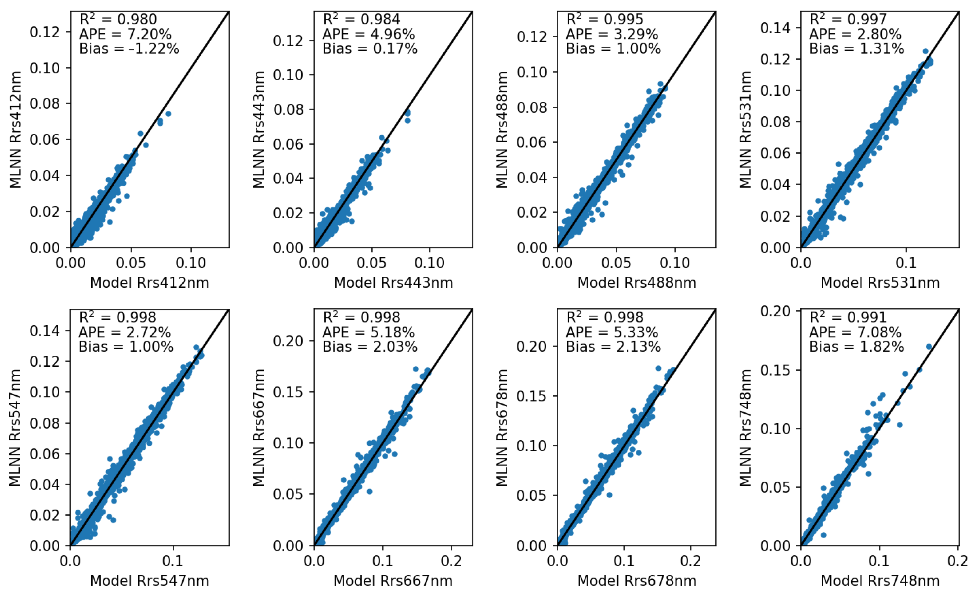
2.3. Algorithm Validation

The performance of our MLNN algorithms was first evaluated with a synthetic dataset. We randomly selected 90% of the synthetic dataset to train the ($R_{\mathrm{rs}}$) neural networks, the remaining 10% of the data were used to evaluate the trained neural networks. For the $R_{\mathrm{rs}}$ MLNN the $R^2$ was higher than 0.993 for all visible bands (412, 443, 488, 531, 547, 667, and 678 nm) and the APD was <5.4%. These results imply that the $R_{\mathrm{rs}}$ MLNN algorithms have learned the radiative transfer inversion process very accurately. In other words, they have learned the spectral relationship between $L_{rc}$($\lambda$) and $R_{\mathrm{rs}}$($\lambda$). The $R_{\mathrm{rs}}$ MLNN algorithm was also validated by comparing its retrieval performance to SeaDAS NIR, SeaDAS NIR/SWIR, and C2RCC algorithms for a large set of ocean color data. For water-leaving radiance retrievals, the MLNN algorithm has the best performance, especially in the blue bands. On average, at 412 nm, the MLNN algorithm reduced APD by 13.4%, 9.6%, and 8.8% compared with the NIR, NIR/SWIR, and C2RCC algorithms, respectively. Furthermore, the NIR algorithm produced more than 17% negative $n{L}_w$ values in blue and red bands and the NIR/SWIR algorithm produced approximately 15% negative $n{L}_w$ values in those bands. In contrast, our neural network-based MLNN (OC-SMART) algorithm and the C2RCC algorithm did not produce any negative $n{L}_w$ values.

2.4. Application

Currently OC-SMART supports ocean color data retrievals from 11 multi-spectral and hyper spectral sensors onboard satellites operated by the National Aeronautics and Space Administration (NASA), the National Oceanic and Atmospheric Administration (NOAA), the European Space Agency (ESA), the Japan Aerospace Exploration Agency (JAXA), the Korea Institute of Ocean Science and Technology (KIOST), and the China Meteorological Administration (CMA), which include SeaStar/SeaWiFS (NASA), MODIS/Aqua (NASA), SNPP/VIIRS (NASA/NOAA), ISS/HICO (NASA), Landsat8/OLI (NASA), DSCOVR/EPIC (NOAA), Sentinel-2/MSI (ESA), Sentinel-3/OLCI (ESA), GCOM-C/SGLI (JAXA), COMS/GOCI (NASA), and FengYun-3D/MERSI (CMA). The performance of OC-SMART was first tested using an independent synthetic testing dataset. Then the ocean color products retrieved by OC-SMART were validated against in situ measurements from MOBY [38], SeaBASS [39], and AERONET-OC [40] data for several sensors.

As alluded to in Section 1, it is important to address uncertainties on a pixel by pixel basis for satellite retrievals to gain confidence in the inferred results. This task is difficult for a neural network designed as a regressor, which generally returns a single predicted value instead of a probability distribution. To form uncertainty estimates on a pixel by pixel basis we have adopted a Bayesian approach in which uncertainties of measured TOA radiances and a priori information are used to quantify uncertainties in the retrieval parameters delivered by OC-SMART. This approach is described in detail in Section 3 with a summary of the processing chain illustrated in Figure 1 of Section 3.5 and with application of this approach shown for various regions and several sensors in Section 4.

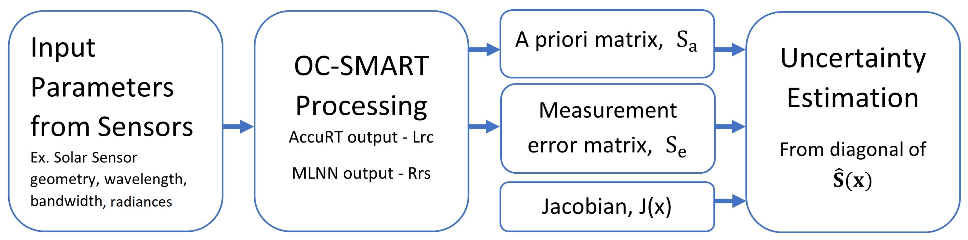
3. Methodology for Quantifying Uncertainties

3.1. Bayesian Inversion

The Bayesian approach is summarized in this Section [24,41,42]. To generate uncertainties for each individual pixel Bayesian inference utilizes measured TOA radiances and a priori data to estimate posterior probability density functions and associated uncertainties. Bayes’ theorem can be expressed as:

$$P\left(\mathbf{x}\right|\mathbf{y})=\frac{P\left(\mathbf{y}\right|\mathbf{x})·P(\mathbf{x})}{P\left(\mathbf{y}\right)}.$$

(1)

Here $P\left(\mathbf{x}\right|\mathbf{y})$ describes the posterior probability density function (pdf) of the state parameters assembled in the vector $\mathbf{x}$ given the measurements assembled in the vector $\mathbf{y}$. $P\left(\mathbf{y}\right|\mathbf{x})$ describes $\mathbf{y}$ if the state were $\mathbf{x}$, $P\left(\mathbf{x}\right)$ is the estimate of the probability of $\mathbf{x}$ before the $\mathbf{y}$ data are observed. Bayes’ theorem allows a process to inversion by updating $P\left(\mathbf{x}\right)$ with the measurement pdf $P\left(\mathbf{y}\right|\mathbf{x})$ to calculate $P\left(\mathbf{x}\right|\mathbf{y})$.

Experimental error is frequently described by a normal distribution [41]. Therefore, for simplicity and convenience, we will assume that each pdf is a Gaussian distribution, which, for an arbitrary vector $\mathbf{z}$, can be expressed as:

$$P\left(\mathbf{z}\right)=\frac{1}{{\left(2\pi \right)}^{1/2}{\left[{\mathbf{S}}_z\right]}^{1/2}}exp[-\frac{1}{2}{(\mathbf{z}-\widehat{\mathbf{z}})}^T{\mathbf{S}}_z^{-1}(\mathbf{z}-\widehat{\mathbf{z}})].$$

(2)

Here, $\widehat{\mathbf{z}}$ is the expected value of $\mathbf{z}$ and ${\mathbf{S}}_z$ is the covariance matrix. If the forward model $\mathbf{F}\left(\mathbf{x}\right)$ can be linearized, then we have

$$\mathbf{y}=\mathbf{F}\left(\mathbf{x}\right)+\mathbf{e}\approx \mathbf{Jx}+\mathbf{e}$$

(3)

where $\mathbf{J}$ is the Jacobian matrix [see Equation (11)] and e represents random measurement uncertainty. In the linear case, we can obtain an explicit retrieval, such as the expected value, by choosing a suitable state, such as the most probable state determined from the posterior pdf $P\left(\mathbf{x}\right|\mathbf{y})$. We do not expect our problem to be linear, but Equation (3) introduces the Jacobian which will be used in the general non-linear case. Hence, in the non-linear case we proceed as follows.

Taking the logarithm of Equation (1) we have:

$$2lnP\left(\mathbf{x}\right|\mathbf{y})\propto lnP(\mathbf{y}\left|\mathbf{x}\right)+lnP\left(\mathbf{x}\right).$$

(4)

Again, if all pdf’s are assumed to be Gaussian, then Equation (4) can be written (see Appendix A for a derivation)

$$ln\left[P\left(\mathbf{x}\right|\mathbf{y})\right]\propto {(\mathbf{y}-\mathbf{F}\left(\mathbf{x}\right))}^T{{\mathbf{S}}_{\mathbf{e}}}^{-1}(\mathbf{y}-\mathbf{F}\left(\mathbf{x}\right))+{(\mathbf{x}-{\mathbf{x}}_{\mathbf{a}})}^T{{\mathbf{S}}_{\mathbf{a}}}^{-1}(\mathbf{x}-{\mathbf{x}}_{\mathbf{a}})$$

(5)

where $\mathbf{F}\left(\mathbf{x}\right)$ is the non-linear forward model, ${\mathbf{S}}_{\mathbf{e}}$ is the measurement error covariance matrix, and ${\mathbf{S}}_{\mathbf{a}}$ is the a priori covariance matrix [41,42]. The right hand side of Equation (5) represents the cost function which must be minimized in order to solve the inverse problem. In the non-linear case an explicit solution is not available. The solution can be determined iteratively using the Gauss–Newton method:

$${\mathbf{x}}_{i+1}={\mathbf{x}}_i+{({\mathbf{J}}_i^T{{\mathbf{S}}_{\mathbf{e}}}^{-1}{\mathbf{J}}_i+{{\mathbf{S}}_{\mathbf{a}}}^{-1})}^{-1}[{\mathbf{J}}_i^T{{\mathbf{S}}_{\mathbf{e}}}^{-1}(\mathbf{y}-\mathbf{F}\left({\mathbf{x}}_i\right))-{{\mathbf{S}}_{\mathbf{a}}}^{-1}({\mathbf{x}}_i-{\mathbf{x}}_{\mathbf{a}})].$$

(6)

Upon convergence to the state vector $\mathbf{x}$, the posterior error covariance matrix becomes:

$$\widehat{\mathbf{S}}\left(\mathbf{x}\right)={(\mathbf{J}{\left(\mathbf{x}\right)}^T{{\mathbf{S}}_{\mathbf{e}}}^{-1}\mathbf{J}\left(\mathbf{x}\right)+{{\mathbf{S}}_{\mathbf{a}}}^{-1})}^{-1}.$$

(7)

The evaluation of each of these matrices is discussed in the following sections. By taking the square root of the diagonal elements of $\widehat{\mathbf{S}}\left(\mathbf{x}\right)$, we arrive at the standard uncertainty estimate of the posterior:

$$\sigma =\sqrt{\mathrm{diag}\left(\widehat{\mathbf{S}}\left(\mathbf{x}\right)\right)}.$$

(8)

Equation (6) implies that the state vector $\mathbf{x}$ is changed iteratively until convergence is reached. This optimal estimation process can be time consuming and computationally taxing, and may not converge if the initial guess of $\mathbf{x}$ is too far from the true value. As explained in Section 3.1.1 below, the OC-SMART approach uses a multi-layer neural network (MLNN) to solve the inverse problem. The benefit of this approach is that once the neural network is properly trained it should give a result that is as good as that obtained by the Gauss–Newton method, but in a significantly shorter computational time. The MLNN approach solves the inverse problem (rather than iteratively as in the Gauss–Newton method) by a training procedure that typically involves the solution of numerous non-linear inversion problems using the gradient descent method to optimize the weights and biases in the neural network (see Equation (10) below).

For our purposes, sensor L1B calibrated radiances and sun-satellite geometry data are processed by OC-SMART to yield the desired retrieval parameters. These L2 retrieval parameters are inserted into the forward model and used to compute simulated Rayleigh-corrected TOA radiances, as explained in some detail in Section 3.1.1 below. The difference between the simulated and measured radiance is calculated for all wavelengths and if the mean of these differences is lower than an acceptable threshold of 10% we consider the retrieval parameters for this pixel to be converged, as illustrated in Figure 2. The application of this convergence check indicates that pixels for which the retrieval values have not converged are usually found in optically complex areas, such as bays and inlets, as well as in the proximity of cloud-contaminated pixels.

3.1.1. Convergence Check

As alluded to above, sensor L1B Rayleigh-corrected radiances and sun-satellite geometry data comprise the measurement vector $\mathbf{y}$ used as input to OC-SMART, which after processing, will return L2 data as retrievals as explained elsewhere [13]. Using MODIS as an example case, we used reflectance measurements in 8 channels (412, 443, 488, 531, 547, 667, 748, and 869 nm), and 3 geometry angles (solar zenith angle, sensor viewing angle, and relative azimuth angle) as the input layer elements (a total of 11 input elements). A specific MLNN was constructed and trained to retrieve $R_{\mathrm{rs}}$ estimates at these eight wavelengths. The transfer (activation) function of the neurons was taken to be the hyperbolic tangent function:

$$f\left(x\right)=\frac{2}{1+\exp [-2x]}-1=\frac{e^x-e^{-x}}{e^x+e^{-x}}=tanh\left(x\right).$$

(9)

In the output layer, a linear transfer function is used to link the hidden layers to the output. The exact expression of this MLNN can be written as

$${\displaystyle y_m=b_{4,m}+\sum _{l=1}^{N_3}{w}_{4,ml}·f\left\{b_{3,l}+\sum _{k=1}^{N_2}{w}_{3,lk}·f\left[b_{2,k}+\sum _{j=1}^{N_1}{w}_{2,kj}·f\left(b_{1,j}+\sum _{i=1}^{N_0}{w}_{1,ji}·x_i\right)\right]\right\}}$$

(10)

where $x_i$, $i=1,\dots ,N_0$ is an element in the input layer.

It is important to note that if the goal is to make a retrieval of state parameters directly from TOA reflectance measurements, then the input parameters $x_i$ in Equation (10) are the measured TOA reflectances at the chosen sensors channels plus the three solar/viewing geometry angles, while the output parameters $y_m$ are the desired retrieval (state) parameters, which, in our above example case, are the $R_{\mathrm{rs}}$ estimates in the eight MODIS channels. We shall refer to this MLNN as R2P (Radiance → Parameter) for short.

On the other hand, if the goal is to use the MLNN [Equation (10)] as a fast interpolator to obtain the TOA radiances and associated Jacobians, then the input parameters $x_i$ should be the state parameters and the solar/viewing geometry, and the output parameters $y_m$ should be the TOA radiances [42]. We shall refer to this MLNN as P2R (Parameter → Radiance) for short.

In Equation (10), $w_{1,ji}$, $w_{2,kj}$, $w_{3,lk}$, and $w_{4,ml}$ are the weights of the three hidden layers and the output layer, and $b_{1,j}$, $b_{2,k}$, $b_{3,l}$, and $b_{4,m}$ are the biases of the three hidden layers and the output layer. The weights and biases are to be determined by the training. f is the hyperbolic tangent function in Equation (9). $y_m$ is the mth element in the output layer, which, in the P2R case, consists of the atmospheric and water IOP retrieval parameters retrieved by OC-SMART. As explained at the end of Section 3.1, the P2R MLNN was used to compute TOA radiances from the retrieval parameters, and a comparison of these computed TOA radiances with the measured ones was used to check the convergence of the retrieval parameters produced by OC-SMART.

3.1.2. Evaluation of the Jacobian

The Jacobian matrix in Equations (3) and (7) for an $m\times n$ matrix can be expressed as

$$\mathbf{J}=\left[\begin{array}{ccc}\frac{\partial \mathbf{F}\left({\mathbf{x}}_{\mathbf{1}}\right)}{\partial {\mathbf{x}}_{\mathbf{1}}}& \cdots & \frac{\partial \mathbf{F}\left({\mathbf{x}}_{\mathbf{1}}\right)}{\partial {\mathbf{x}}_{\mathbf{n}}}\\ ⋮& \ddots & ⋮\\ \frac{\partial \mathbf{F}\left({\mathbf{x}}_{\mathbf{m}}\right)}{\partial {\mathbf{x}}_{\mathbf{1}}}& \cdots & \frac{\partial \mathbf{F}\left({\mathbf{x}}_{\mathbf{m}}\right)}{\partial {\mathbf{x}}_{\mathbf{n}}}\end{array}\right]$$

(11)

where $\mathbf{F}\left(\mathbf{x}\right)$ is the forward model and $\mathbf{x}$ is the state vector [see Equation (3)]. For the Jacobians we need the partial derivatives in Equation (11), which can be calculated analytically or closely approximated by using finite differences. In our testing we found that the two methods produced identical values for uncertainties out to several decimal places. Because of the closeness of values produced by the two methods, the finite difference method was chosen for use in this paper, because it was found to reduce the computation time.

3.2. Measurement Error

The measurement error covariance matrix ${\mathbf{S}}_{\mathbf{e}}$ stems from the uncertainties of the measurement instrument. $R_{\mathrm{rs}}$ is derived from the Rayleigh-corrected TOA radiances $L_{rc}$ which are measured by ocean color satellite sensors. Our measurement error would then come from the per-pixel radiometric uncertainty for satellite L1B data. This information is currently not available because it is difficult to model noise from photonic, detector, and electronic sources [43]. Therefore, we assumed the value of one percent for radiometric uncertainty because it is consistent with Gaussian noise added to the OC-SMART neural network training dataset. Details on the neural network training data, such as formation, testing, and validation are discussed elsewhere [14].

The measurement error covariance matrix ${\mathbf{S}}_{\mathbf{e}}$ is calculated by taking the square of 1% of the Rayleigh-corrected TOA radiances $L_{rc}$.

$${\mathbf{S}}_{\mathbf{e}}=0.{01}^2\times {L_{rc}}^2.$$

(12)

This value is likely a conservative estimate of radiometric uncertainty. The use of signal to noise ratios as an adequate uncertainty has been criticized [43,44] because it is not rigorously quantified and does not provide any information on possible spectral covariance in the radiometric noise. These are valid concerns and are topics of ongoing investigations within the ocean color remote sensing community. We have chosen to define measurement error as stated above because it is applicable to all sensors compatible with OC-SMART.

3.3. A Priori Estimation

The a priori stems from our general knowledge of the uncertainties, and can be estimated as a covariance matrix

$${\mathbf{S}}_{\mathbf{a}}={{\sigma }_a}^2.$$

(13)

where ${\sigma }_a$ represents the standard deviations of the a priori. To estimate ${\sigma }_a$, we compare the MLNN predictions (Figure 3) with a training dataset comprised of synthetic data. From this comparison, we take the average percent error (APE) for each $R_{\mathrm{rs}}$ wavelength band. These APEs are multiplied by the corresponding retrieval values ${\mathbf{x}}_{Ret}$ to form ${\sigma }_a=\mathrm{APE}\times {\mathbf{x}}_{Ret}$. This approach follows the standard procedure for choosing good a priori values [45,46]. Using this estimate of ${\sigma }_a$ we can rewrite Equation (13) as:

$${\mathbf{S}}_{\mathbf{a}}={\mathrm{APE}}^2\times {{\mathbf{x}}_{Ret}}^2.$$

(14)

As a note, the a priori estimate can be expressed in different ways as it is simply a representation of our prior knowledge. We have chosen to define the a priori as stated above. If, however, a better (more complete) knowledge of the uncertainty becomes available the estimate of the a priori can be adapted to accommodate this updated information.

Figure 3. Verification of the remote sensing reflectance ($R_{\mathrm{rs}}$) at 412, 443, 488, 531, 547, 667, 678, and 748 nm retrieved by the MLNN algorithm against a synthetic testing dataset (N = 10,000).

Figure 3. Verification of the remote sensing reflectance ($R_{\mathrm{rs}}$) at 412, 443, 488, 531, 547, 667, 678, and 748 nm retrieved by the MLNN algorithm against a synthetic testing dataset (N = 10,000).

3.4. Special Cases

Let us now consider the special case of Equation (7): $\widehat{\mathbf{S}}\left(\mathbf{x}\right)={(\mathbf{J}{\left(\mathbf{x}\right)}^T{{\mathbf{S}}_{\mathbf{e}}}^{-1}\mathbf{J}\left(\mathbf{x}\right)+{{\mathbf{S}}_{\mathbf{a}}}^{-1})}^{-1}$. If the measurement error term, $\mathbf{J}{\left(\mathbf{x}\right)}^T{{\mathbf{S}}_{\mathbf{e}}}^{-1}\mathbf{J}\left(\mathbf{x}\right)$, approaches zero then Equation (7) becomes:

$$\widehat{\mathbf{S}}\left(\mathbf{x}\right)\approx {\mathbf{S}}_{\mathbf{a}}.$$

(15)

This would cause the standard uncertainty estimate of the posterior to become:

$${\sigma }_a\approx \sqrt{\mathrm{diag}({\mathbf{S}}_{\mathbf{a}}.)}\approx \mathrm{APE}\times {\mathbf{x}}_{Ret}.$$

(16)

This simplified case, i.e., Equation (16), is in essence the same as the approach used by the C2RCC [25] and SWARM [26] algorithms to attach uncertainties to IOPs. If the diagonal elements of the measurement error term are positive then:

$$\mathrm{diag}\left[{(\mathbf{J}{\left(\mathbf{x}\right)}^T{{\mathbf{S}}_{\mathbf{e}}}^{-1}\mathbf{J}\left(\mathbf{x}\right)+{{\mathbf{S}}_{\mathbf{a}}}^{-1})}^{-1}\right]<\mathrm{diag}\left[{\mathbf{S}}_{\mathbf{a}}\right],$$

(17)

which would lead to a smaller uncertainty than implied by Equation (16). From testing we found that the partial derivative of the forward model, $\mathbf{F}\left(\mathbf{x}\right)$, and state vector, $\mathbf{x}$, produced values near zero causing the measurement error term to result in a positive value near zero. This circumstance also makes it less important to have the best approach for forming the measurement error covariance matrix term, ${\mathbf{S}}_{\mathbf{e}}$, as it will be effectively neutralized by the Jacobian, $\mathbf{J}\left(\mathbf{x}\right)$.

3.5. Experimental Setup

Figure 1 shows a flowchart of the processing chain described in Section 3.1, Section 3.2, Section 3.3. For an example case, such as that described in Section 4.1, MODIS L1B radiances and sun-satellite geometry data are used as inputs to OC-SMART which will then produce L2 retrievals of $R_{\mathrm{rs}}$ used to form the a priori matrix ${\mathbf{S}}_{\mathbf{a}}$, and Rayleigh-corrected radiances used to form the measurement error matrix ${\mathbf{S}}_{\mathbf{e}}$. These matrices, along with the Jacobian, are used to form the posterior error covariance matrix $\widehat{\mathbf{S}}\left(\mathbf{x}\right)$ [see Equation (7)], and by taking the diagonal of this matrix we arrive at an estimate of corresponding $R_{\mathrm{rs}}$ uncertainties. This experimental setup can be viewed as a framework that can easily be adapted to other sensors, such as those listed in Section 2.4, by substituting those sensors TOA radiance and geometry data in place of MODIS data.

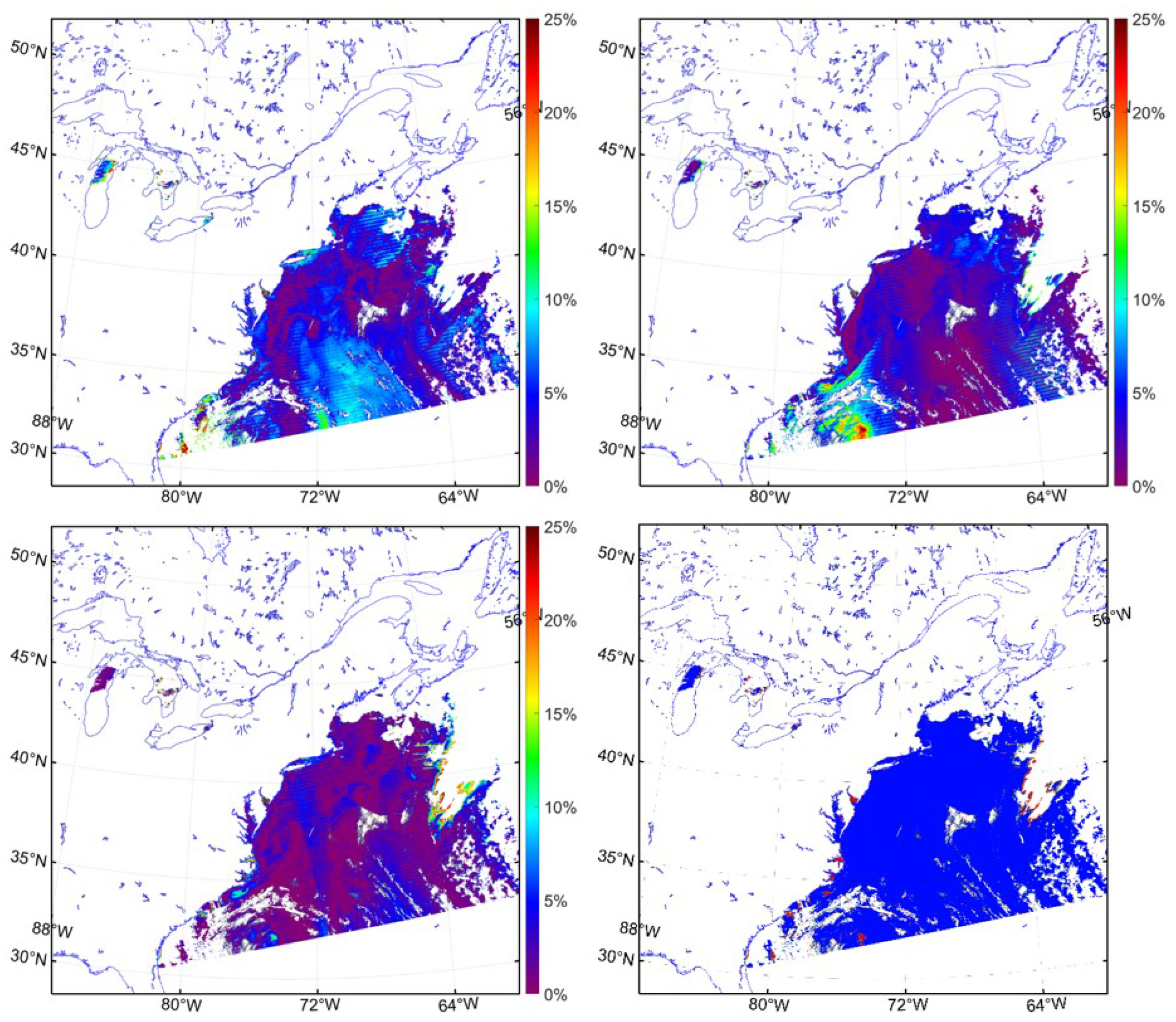
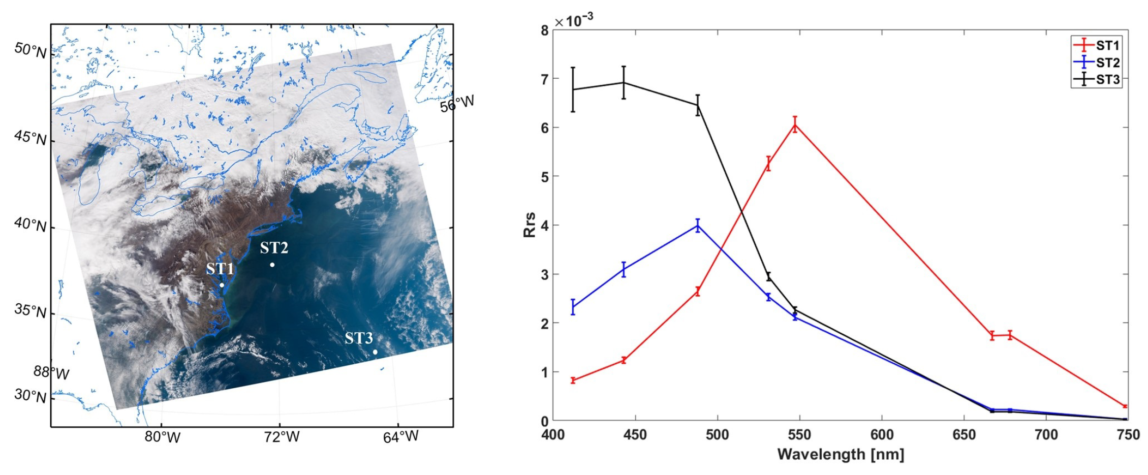
4. Case Studies and Discussion

4.1. Application to MODIS

Using MODIS Aqua L1B calibrated radiances and sun-satellite geometry data with 1 km resolution as inputs to OC-SMART, we produced L2 retrievals of $R_{\mathrm{rs}}$ and corresponding $R_{\mathrm{rs}}$ uncertainty estimates. For demonstration purposes, we now consider three different geographical locations. These locations are the east coast of the United States (Figure 4 and Figure 5), the Gulf of Mexico (Figure 6 and Figure 7), and the East Coast of China (Figure 8 and Figure 9). Figure 4, Figure 5, Figure 6, Figure 7 and Figure 8 show RGB images of the locations being considered, as well as $R_{\mathrm{rs}}$ estimates with error bars for these locations. A more holistic view of the $R_{\mathrm{rs}}$ estimates and their corresponding uncertainties (standard deviations) and relative uncertainties (ratio of the uncertainty to the measured quantity) are shown for several wavelengths in Figure 5, Figure 6, Figure 7, Figure 8 and Figure 9.

Figure 4 shows an RGB image of the eastern coast of the United States along with three locations of interest. ST1 and ST2 are located in optically complex waters off the coast, with ST1, in particular, being located in the Chesapeake Bay region where waters are extremely turbid. This turbidity is reflected by the elevated $R_{\mathrm{rs}}$ in the green bands for ST1. We would expect to see larger uncertainties in bands with weaker signals because noise is more prevalent. As waters are primarily blue, these larger uncertainties due to noise should be more prevalent in the green and red bands. However, the right panel of Figure 4 tells a different story. Here, we see that the largest uncertainties are more closely associated with larger $R_{\mathrm{rs}}$ estimates.

To explain this behavior, let us first examine the terms of the posterior error covariance matrix Equation (see Equation (7)). As explained in Section 3.4, the measurement error covariance matrix term, ${\mathbf{S}}_{\mathbf{e}}$ is effectively neutralized by the Jacobian leading to the a priori term dominating to such an extent that if the measurement error term were considered to be zero the calculation of uncertainty would not be significantly changed, as seen in Figure 10B. In fact this scenario would be in line with the approach used by the C2RCC [25] and SWARM [26] algorithms to attribute uncertainties to IOPs. Without the measurement term, the posterior error covariance matrix can in essence be simplified to a weighted average percent difference between estimated $R_{\mathrm{rs}}$ retrievals and training simulation data.

With this situation in mind now consider our definition of the a priori in Equation (14). We have defined it to be a combination of the retrieval parameters ($R_{\mathrm{rs}}$ estimates in this case) and average percent errors (APEs), as determined in Section 3.3. Equation (14) implies that the largest uncertainties should occur in bands where both the $R_{\mathrm{rs}}$ and the APEs are large. The APEs associated with each $R_{\mathrm{rs}}$ wavelength in Figure 3 are higher for blue bands than for red bands with green bands exhibiting the lowest APEs, meaning that even if the $R_{\mathrm{rs}}$ estimates were equal for blue and green bands we should expect larger uncertainty estimates in the blue bands. This finding is consistent with the findings reported by others [22,47] based on an optimal estimation approach. Equation (14) also explains why we are seeing small uncertainties in red bands, because the $R_{\mathrm{rs}}$ estimates are almost always lower in those bands than in the blue and green bands.

Figure 10 shows the $R_{\mathrm{rs}}$ and uncertainty estimates for the three locations identified in Figure 4. Figure 10A shows the calculated uncertainties estimates while Figure 10B shows the same uncertainty calculation if the measurement error term was set to zero. As stated above, setting the error measurement term to zero hardly makes an impact on the uncertainties. Figure 10C shows the uncertainty calculation if all the APE values were set to 10%, which would imply a poorer match-up of the trained MLNN to the synthetic data. On the other hand, lower APEs would have implied a better match-up and would lead to lower uncertainty estimates. This finding emphasizes the importance of a well-trained neural network. The a priori plays a very significant role in determining the uncertainty estimate and is largely tied to the value of $R_{\mathrm{rs}}$ at each pixel. This situation leads to a nearly constant relative uncertainty which closely mirrors the APE value for each wavelength. Had the measurement error term played a larger role, we would have expected to see more variability in the relative uncertainty.

When looking at the Gulf of Mexico in Figure 6 we can see a similar shape of the $R_{\mathrm{rs}}$ estimate curves for ST4 and ST5, as was seen in Figure 4, for the ST3 location in the open ocean. The ST5 $R_{\mathrm{rs}}$ curve, however, has an elevated green band profile comparable to, though not as dramatic, as that of ST1 in the Chesapeake Bay. The uncertainties for ST5 demonstrate the importance of the APE values. Even though we see higher $R_{\mathrm{rs}}$ estimates in green bands than blue, the blue bands still have larger uncertainties because of their higher APEs. OC-SMART is based on simulated datasets for optically deep water and while it can be applied to coastal regions where shallow waters are present, the waters must be optically deep for OC-SMART to return accurate simulated radiances. For this reason we are able to make realistic simulations at ST5 where waters are turbid and, therefore, optically deep but not near the Bahamas where the waters are clearer and, therefore, optically shallower even though the areas have similar physical ocean depths. For those interested in what optically shallow results might look like we refer to Figure 7, where a drastic difference in $R_{\mathrm{rs}}$ and uncertainty is evident near the Bahamas, Cuba, and the Yucatan Peninsula where the shallow, clear waters of these regions allow for light to be reflected off the bottom of the ocean leading to enhanced $R_{\mathrm{rs}}$ estimates.

The RGB image in Figure 8 shows a green complexion around ST7 near the Korean peninsula which unsurprisingly leads to the elevated green bands of the $R_{\mathrm{rs}}$ curve. The $R_{\mathrm{rs}}$ estimate curve at ST6 has a similar shape to that of ST3 in the open ocean although the $R_{\mathrm{rs}}$ estimates are lower at ST6 than those seen in Figure 4 and Figure 6, as this region is closer to the coast and has more complex waters as can be observed in Figure 9.

4.2. Application to Other Sensors

The methodology laid out above can easily be applied to other ocean color sensors. Modifications to the experimental setup described in Section 3.5 are minor and include modifying the forward model to be suitable for a specific sensor and adjusting the wavelength bands and APEs. Shown here are results from the OLCI Sentinel-3 sensor off the Iberian peninsula (Figure 11 and Figure 12) and the VIIRS sensor over the Atlantic ocean (Figure 13 and Figure 14). Similar to MODIS sensor data in Figure 8, OLCI sensor data in Figure 11 show elevated green bands for optically complex coastal water. In this case, run-off from two prominent rivers lead to the results for ST8 while larger blue band values are observed in the open ocean region of ST9. A compilation of $R_{\mathrm{rs}}$ estimate retrievals and uncertainties for this region are provided in Figure 12. In the RGB image of Figure 13, VIIRS sensor data for ST10 and ST11 closely match those of ST2 and ST3 in Figure 5. Despite the presence of sunglint in the region $R_{\mathrm{rs}}$ retrievals and uncertainties are largely unaffected as can be seen in Figure 14.

The locations of interest shown for various regions and several sensors are intended to provide insight on a variety of water conditions beyond the open ocean where OC-SMART and other AC algorithms perform best. The OC-SMART approach currently uses a large ensemble of IOP realizations in order to represent open ocean water, as well as turbid coastal waters. It is designed to provide a smooth, seamless transition between clear open ocean and turbid coastal waters. Although adequate for many coastal regions, additional IOP data may be needed to obtain more accurate results in some optically complex coastal regions. To improve the performance of OC-SMART in such regions, more IOP data could be added to improve the response/output of OC-SMART. Introducing additional IOP modeling data is also expected to improve the uncertainty estimations discussed in this paper as it would allow use of more adaptive a priori assessments and measurement error calculations.

5. Conclusions and Perspectives

We have successfully implemented a method based on Bayes’ theorem to estimate uncertainties associated with OC-SMART remote sensing reflectance ($R_{\mathrm{rs}}$) retrievals. The OC-SMART platform uses a multi-layer neural network to solve the inverse problem, which saves significant calculation time when compared to typical Bayesian (optimal estimation) approaches. This methodology was applied to MODIS, OLCI, and VIIRS sensor data in various optically complex regions and $R_{\mathrm{rs}}$ retrievals with corresponding uncertainties were presented and discussed for these locations. The uncertainty estimates were dominated by the a priori term, leading to a strong connection between large uncertainties and large $R_{\mathrm{rs}}$ and APE values.

This framework for uncertainty estimation could be expanded to include other OC-SMART retrievals, such as aerosol optical depth, chlorophyll concentration, absorption coefficients, and backscattering coefficients. The inclusion of uncertainty estimates for aerosol optical depths, in particular, would involve only minor changes to the methods described in this paper, namely adjustments to the APE values in the a priori term. For other retrieval parameters, such as chlorophyll concentrations and water IOPs new considerations will have to made for determining measurement errors and a priori, as well as calculations of the Jacobian. MODIS, OLCI, and VIIRS sensor data were used in this paper, but the calculations of uncertainties could also be performed for any sensor that OC-SMART is compatible with those mentioned in Section 2.

Improvements could be made to our estimations by obtaining better information on the a priori. In our case, such improvement would imply a better match-up of MLNN retrievals to synthetic data which could be achieved by implementing additional IOP data to the training dataset of the neural network. We could also improve estimations if uncertainties associated with satellite radiance measurements were available. Such information would allow us to apply measurement error terms more accurately than assuming one percent Gaussian noise for all bands. Future work would include an expansion of our approach to encompass all applicable OC-SMART retrievals and to integrate uncertainty estimation into the currently available Python OC-SMART package and plug-ins.

References

1. Nieke, J.; Borde, F.; Mavrocordatos, C.; Berruti, B.; Delclaud, Y.; Riti, J.B.; Garnier, T. The Ocean and Land Colour Imager (OLCI) for the Sentinel 3 GMES Mission: Status and first test results. In Proceedings of the Earth Observing Missions and Sensors: Development, Implementation, and Characterization II, Kyoto, Japan, 30 October–1 November 2012. [Google Scholar]
2. Frerick, J.; Mavrocordatos, C.; Berruti, B.; Donlon, C.; Cosi, M.; Engel, W.; Bianchi, S.; Smith, S. Next generation along track scanning radiometer—SLSTR. In Proceedings of the Remote Sensing System Engineering IV, San Diego, CA, USA, 12–16 August 2012; Volume 8516. [Google Scholar]
3. Wang, M. (Ed.) Atmospheric Correction for Remotely-Sensed Ocean-Colour Products; Technical Report; International Ocean Colour Coordinating Group (IOCCG): Dartmouth, NS, Canada, 2010. [Google Scholar]
4. Gordon, H.; Wang, M. Retrieval of water-leaving radiance and aerosol optical thickness over the oceans with SeaWiFS: A preliminary algorithm. Appl. Opt. 1994, 33, 443–452. [Google Scholar] [CrossRef]
5. O’Reilly, J.; Maritorena, S.; Mitchelle, B.; Siegel, D.; Carder, K.; Garver, S.; Kahru, M.; McClain, C. Ocean colour chlorophyll algorithms for SeaWIFS. J. Geophys. Res. 1998, 103, 24937–24953. [Google Scholar] [CrossRef] [Green Version]
6. Fichot, C.; Downing, B.; Bergamschi, B.; Windham-Myers, L.; Marvin-DiPasquale, M.; Thompson, D.; Gierach, M. High-resolution remote sensing of water quality in the San Francisco Bay–Delta Estuary. Environ. Sci. Technol. 2016, 50, 573–583. [Google Scholar] [CrossRef]
7. Kudela, R.; Palacios, S.; Austerberry, D.; Accorsi, E.; Guild, L.; Torres-Perez, J. Application of hyperspectral remote sensing to cyanobacterial blooms in inland waters. Remote. Sens. Environ. 2015, 167, 196–205. [Google Scholar] [CrossRef] [Green Version]
8. Platt, T.; Hoepffner, N.; Stuart, V.; Brown, C. Why Ocean Colour? The Societal Benefits of Ocean-Colour Technology; Technical Report; International Ocean Colour Coordinating Group (IOCCG): Dartmouth, NS, Canada, 2008. [Google Scholar]
9. Greb, S.; Dekkler, A.; Binding, C. Earth Observations in Support of Global Water Quality Monitoring; Technical Report; International Ocean Colour Coordinating Group (IOCCG): Dartmouth, NS, Canada, 2018. [Google Scholar]
10. Joint Committee for Guides in Metrology. JCGM 100: Evaluation of Measurement Data—Guide to the Expression of Uncertainty in Measurement. 2008, pp. 1–120. Available online: https://www.sci.utah.edu/~kpotter/Library/Papers/jcgm:2008:EMDG/index.html (accessed on 23 May 2023).
11. Scheidt, C.; Li, L.; Caers, J. Quantifying Uncertainty in Subsurface Systems; John Wiley & Sons, American Geophysical Union: Washington, DC, USA, 2018. [Google Scholar]
12. Yang, L.; Hyde, D.; Grujic, O.; Scheidt, C.; Caers, J. Assessing and visualizing uncertainty of 3D geological surfaces using level sets with stochastic motion. Comp. Geosci. 2019, 122, 54–67. [Google Scholar] [CrossRef]
13. Fan, Y.; Li, W.; Gatebe, C.; Jamet, C.; Zibordi, G.; Schroeder, T.; Stamnes, K. Atmospheric correction over coastal waters using multilayer neural networks. Remote. Sens. Environ. 2017, 199, 218–240. [Google Scholar] [CrossRef]
14. Fan, Y.; Li, W.; Chen, N.; Ahn, J.; Park, Y.; Kratzer, S.; Schroeder, T.; Ishizaka, J.; Chang, R.; Stamnes, K. OC-SMART: A machine learning based data analysis platform for satellite ocean color sensors. Remote. Sens. Environ. 2021, 253, 112236. [Google Scholar] [CrossRef]
15. Moore, G.; Aiken, J.; Lavender, S. The atmospheric correction of water color and the quantitative retrieval of suspended particulate matter in Case II waters: Application to MERIS. Int. J. Remote. Sens. 1999, 20, 1713–1733. [Google Scholar] [CrossRef]
16. Bailey, S.; Franz, B.; Werdell, P. Estimation of near-infrared water-leaving reflectance for satellite ocean color data processing. Opt. Express 2010, 18, 7521–7527. [Google Scholar] [CrossRef]
17. Stamnes, K.; Li, W.; Yan, B.; Elde, H.; Barnard, A.; Pegau, S.; Stamnes, J.J. Accurate and selfconsistent ocean color algorithm: Simultaneous retrieval of aerosol optical properties and chlorophyll concentrations. Appl. Opt. 2007, 42, 939–951. [Google Scholar] [CrossRef]
18. Ibramhim, A.; Franz, B.; Ahmad, Z.; Bailey, S. Multiband Atmospheric Correction Algorithm for Ocean Color Retrievals. Front. Earth Sci. 2019, 7, 116. [Google Scholar] [CrossRef]
19. Thompson, D.; Natraj, V.; Green, R.; Helmlinger, M.; Gao, B.; Eastwood, M. Optimal estimation for imaging spectrometer atmospheric correction. Remote. Sens. Environ. 2018, 216, 355–373. [Google Scholar] [CrossRef]
20. Steinmetz, F.; Deschamps, P.; Ramon, D. Atmospheric correction in presence of sun glint: Application to MERIS. Opt. Express 2011, 19, 9783–9800. [Google Scholar] [CrossRef] [Green Version]
21. Doerffer, R.; Schiller, H. The MERIS Case 2 water algorithm. Int. J. Remote. Sens. 2007, 28, 517–535. [Google Scholar] [CrossRef]
22. Thompson, D.; Cawse-Nicholson, K.; Erickson, Z.; Fichot, C.; Frankenberg, C.; Gao, B.-C.; Gierach, M.M.; Green, R.O.; Jensen, D.; Natraj, V.; et al. A unified approach to estimate land and water reflectances with uncertainties for coastal imaging spectroscopy. Remote. Sens. Environ. 2019, 231, 111198. [Google Scholar] [CrossRef] [Green Version]
23. Frouin, R.; Pelletier, B. Bayesian methodology for inverting satellite ocean-color data. Remote Sens. Environ. 2015, 159, 332–360. [Google Scholar] [CrossRef]
24. Feng, R.; Grana, D.; Mukerji, T.; Mosegaard, K. Application of Bayesian generative adversarial networks to geological facies modeling. Math. Geosci. 2022, 54, 831–855. [Google Scholar] [CrossRef]
25. Brockmann, C.; Doerffer, R.; Peters, M.; Stelzer, K.; Embacher, S.; Ruescas, A. Evolution of the C2RCC Neural Network for Sentinel 2 and 3 for the Retrieval of Ocean Colour Products in Normal and Extreme Optically Complex Waters. In Proceedings of the Living Planet Symposium. European Space Agency Special Publication, Prague, Czech Republic, 9–13 May 2016; pp. 1–6. [Google Scholar]
26. Hieronymi, M.; Muller, D.; Doerffer, R. The OLCI Neural Network Swarm (ONNS): A Bio-Geo-Optical Algorithm for Open Ocean and Coastal Waters. Front. Mar. Sci. 2017, 4, 140. [Google Scholar] [CrossRef] [Green Version]
27. Schroeder, T.; Schaale, M.; Lovell, J.; Blondeau-Patissier, D. An ensemble neural network atmospheric correction for Sentinel-3 OLCI over coastal waters providing inherent model uncertainty estimation and sensor noise propagation. Remote. Sens. Environ. 2022, 270, 112848. [Google Scholar] [CrossRef]
28. Ibrahim, A.; Franz, B.; Sayer, A.; Knobelspiesse, K.; Zhang, M.; Bailey, S.; McKinna, L.; Gao, M.; Werdell, J. Optimal estimation framework for ocean color atmospheric correction and pixel-level uncertainty quantification. Appl. Opt. 2022, 61, 6453–6475. [Google Scholar] [CrossRef]
29. Zhang, M.; Ibrahim, A.; Franz, B.; Ahmad, Z.; Sayer, A. Estimating pixel-level uncertainty in ocean color retrievals from MODIS. Opt. Express 2022, 30, 31415–31438. [Google Scholar] [CrossRef]
30. Stamnes, K.; Hamre, B.; Stamnes, S.; Chen, N.; Fan, Y.; Li, W.; Lin, Z.; Stamnes, J. Progress in forward-inverse modeling based on radiative transfer tools for coupled atmosphere-snow/ice-ocean systems: A review and description of the accurt model. Appl. Sci. 2018, 8, 2682. [Google Scholar] [CrossRef] [Green Version]
31. Ahmad, Z.; Franz, B.; McClain, C.; Kwiatkowski, E.; Werdell, J.; Shettle, E.; Holben, B. New aerosol models for the retrieval of aerosol optical thickness and normalized water-leaving radiances from the seawifs and modis sensors over coastal regions and open oceans. Appl. Opt. 2010, 49, 5545–5560. [Google Scholar] [CrossRef]
32. Koepke, P.; Gasteiger, J.; Hess, M. Technical note: Optical properties of desert aerosol with non-spherical mineral particles: Data incorporated to opac. Atmos. Chem. Phys. 2015, 15, 5947–5956. [Google Scholar] [CrossRef] [Green Version]
33. Garver, S.; Siegel, D. Inherent optical property inversion of ocean color spectra and its biogeochemical interpretation: 1. Time series from the sargasso sea. J. Geophys. Res. Ocean. 1997, 102, 18607–18625. [Google Scholar] [CrossRef]
34. Ruddick, K. Due Coastcolour Round Robin Protocol. 2010. Available online: https://www.coastcolour.org/documents/Coastcolour-RRP-v1.2.pdf (accessed on 1 June 2020).
35. Morel, A.; Antoine, D.; Gentili, B. Bidirectional reflectance of oceanic waters: Accounting for raman emission and varying particle scattering phase function. Appl. Opt. 2002, 41, 6289–6306. [Google Scholar] [CrossRef]
36. Chen, S.; Billings, S.; Grant, P. Non-linear system identification using neural networks. Int. J. Control 1990, 51, 1191–1214. [Google Scholar] [CrossRef]
37. D’Alimonte, D.; Zibordi, G. Phytoplankton determination in an optically complex coastal region using a multilayer perceptron neural network. IEEE Trans. Geosci. Remote Sens. 2003, 41, 2861–2868. [Google Scholar] [CrossRef]
38. Clark, D.; Yarbough, M.; Feinholz, M.; Flora, S.; Broenkow, W.; Kim, Y.S.; Johnson, B.C.; Brown, S.W.; Yuen, M.; Mueller, J.L. Moby, a Radiometric Buoy for Performance Monitoring and Vicarious Calibration of Satellite Ocean Color Sensors: Measurement and Data Analysis Protocols; NASA Technical Report; NASA: Washington, DC, USA, 2003.
39. Werdell, P.; Bailey, S.; Franz, B.; Morel, A.; McClain, C. On-orbit vicarious calibration of ocean color sensors using an ocean surface reflectance model. Appl. Opt. 2007, 46, 5649–5666. [Google Scholar] [CrossRef]
40. Zibordi, G.; Melin, F.; Berthon, J.C.; Holben, B.; Slutsker, I.; Giles, D.; D’Alimonte, D.; Vandemark, D.; Feng, H.; Schuster, G.; et al. Aeronet-OC: A network for the validation of ocean color primary products. J. Atmos. Ocean. Technol. 2009, 26, 1634–1651. [Google Scholar] [CrossRef]
41. Rodgers, C.D. Inverse Methods for Atmospheric Sounding: Theory and Practice; World Scientific: London, UK, 2000. [Google Scholar]
42. Stamnes, K.; Stamnes, J. Radiative Transfer in Coupled Environmental Systems: An Introduction to Forward and Inverse Modeling; Wiley-VCH: Weinheim, Germany, 2015. [Google Scholar]
43. Lamquin, N.; Mangin, A.; Mazeran, C.; Bourg, B.; Bruniquel, V.; D’Andon, O. OLCI L2 Pixel-by-Pixel Uncertainty Propagation in OLCI Clean Water Branch; European Space Agancy: Paris, France, 2013; pp. 1–51. [Google Scholar]
44. Gilerson, A.; Herra-Estrella, E.; Foster, R.; Agagliate, J.; Hu, C.; Ibrahim, A.; Franz, B. Determining the Primary Sources of Uncertainty in Retrieval of Marine Remote Sensing Reflectance From Satellite Ocean Color Sensors. Front. Remote. Sens. 2022, 3, 25. [Google Scholar] [CrossRef]
45. Jospin, L.; Buntine, W.; Boussa, F.; Laga, H.; Bennamoun, M. Hands-on Bayesian Neural Networks—A Tutorial for Deep Learning Users. IEEE Comput. Intell. Mag. 2022, 17, 29–48. [Google Scholar] [CrossRef]
46. Gelman, A. Prior Choice Recommendations. 2020. Available online: https://github.com/stan-dev/stan/wiki/Prior-Choice-Recommendations (accessed on 10 December 2020).
47. Hu, C.; Feng, L.; Lee, Z. Uncertainties of SeaWiFS and MODIS remote sensing reflectance: Implications from clear water measurements. Remote. Sens. Environ. 2013, 133, 168–182. [Google Scholar] [CrossRef]
Figure 1. Framework for formulation of the uncertainty estimations applied to OC-SMART.
Algorithms 16 00301 g001
Figure 2. The difference between simulated Rayleigh-corrected TOA radiances and measured Rayleigh-corrected TOA radiances from MODIS represented as a percentage for (Top Left) 412 nm, (Top Right) 531 nm, and (Bottom Left) 667 nm. (Bottom Right) A convergence map of OC-SMART output R rs . In this image, over 95% of the retrieved R rs are converged (shown in blue color). Zones of non-convergence, shown in red, are primarily located in coastal bays and near areas of heavy cloud cover.
Algorithms 16 00301 g002
Figure 4. (Left panel) Locations of interest off the east coast of the United States on 9 March 2016 (MODIS). ST1 (Red) is located in the optically complex Chesapeake bay region, ST2 (Blue) is located in near coastal waters, and ST3 (Black) is located in the open ocean. (Right panel) R rs with uncertainties for three locations of interest and for several wavelengths.
Algorithms 16 00301 g004
Figure 5. Remote sensing reflectance data from MODIS sensor (Left), corresponding standard uncertainties (Center), and relative uncertainty (Right) for several wavelengths off the east coast of the United States on 9 March 2016. Relative uncertainty tends to be consistent for all pixels in a wavelength.
Algorithms 16 00301 g005
Figure 6. (Left panel) Locations of interest in the Gulf of Mexico on 4 March 2020 (MODIS). ST4 (Red) is located in the central gulf region while ST5 (Blue) is located in the coastal waters of southwest Florida. (Right panel) R rs with uncertainties for two locations of interest for several wavelengths.
Algorithms 16 00301 g006
Figure 7. Remote sensing reflectance data from MODIS sensor (Left), corresponding standard uncertainties (Center), and relative uncertainty (Right) for several wavelengths over the gulf of Mexico on 4 March 2020. Elevated values near Cuba and the Bahamas are due to shallow waters where reflection from the ocean bottom should be included (ignored in the current version of OC-SMART).
Algorithms 16 00301 g007
Figure 8. (Left panel) Locations of interest off the east coast of China on 19 March 2016 (MODIS). ST6 (red) is located between Korea and western Japan in the Sea of Japan, ST7 (blue) is located in the East China Sea near the Korean peninsula. (Right panel) R rs with uncertainties for two locations of interest for several wavelengths.
Algorithms 16 00301 g008
Figure 9. Remote sensing reflectance data from MODIS sensor (Left), corresponding standard uncertainties (Center), and relative uncertainty (Right) for several wavelengths near the Korean peninsula and sea of Japan on 19 March 2016.
Algorithms 16 00301 g009
Figure 10. R rs uncertainties for the three locations identified in Figure 4 for several wavelengths. Panel (A) shows the actual calculated uncertainty. Panel (B) shows the same uncertainty calculation but with the measurement term considered to be zero for all values. Panel (C) shows the uncertainty calculation if the APEs of all wavelengths were set to 10%.
Algorithms 16 00301 g010
Figure 11. (Left panel) Locations of interest near the Iberian peninsula on 21 January 2022. ST8 (red) is located in the Golfo de Cadiz near the delta of two prominent rivers, ST9 (black) is located west of Lisbon. (Right panel) R rs from OLCI Sentinel-3 sensor data with uncertainties for two locations of interest for several wavelengths.
Algorithms 16 00301 g011
Figure 12. Remote sensing reflectance data from OLCI Sentinel-3 sensor (Left), corresponding standard uncertainties (Center), and relative uncertainty (Right) for several wavelengths near the Iberian peninsula on 21 January 2022.
Algorithms 16 00301 g012
Figure 13. (Left panel) Locations of interest off Northeast coast of the United States on 2 May 2021. ST10 (red) is located south of Nova Scotia in optically complex waters, ST11 (black) is located in an open region of the Atlantic ocean. (Right panel) R rs from VIIRS sensor data with uncertainties for two locations of interest for several wavelengths.
Algorithms 16 00301 g013
Figure 14. Remote sensing reflectance data from VIIRS sensor (Left), corresponding standard uncertainties (Center), and relative uncertainty (Right) for several wavelengths off the Northeast coast of the United States of America on 2 May 2021.
Algorithms 16 00301 g014
Disclaimer/Publisher’s Note: The statements, opinions and data contained in all publications are solely those of the individual author(s) and contributor(s) and not of MDPI and/or the editor(s). MDPI and/or the editor(s) disclaim responsibility for any injury to people or property resulting from any ideas, methods, instructions or products referred to in the content.