1. Introduction
122 years ago, Hilbert [
1] proposed 23 mathematical problems, of which the second part of the 16th one is to find the maximal number of limit cycles and their relative locations for polynomial vector fields. To date, several thousand articles and studies have been devoted to this problem. The study of dynamical systems includes bifurcation theory with branch catastrophe theory [
2]. See also model in the light of Zeeman’s approach [
3]. Arnold [
4] discussed the catastrophes of the ADE classification, because of their relation with the Lie groups. For more details of the existing important results on the generalized polynomial Lienard differential systems and the limit-cycle bifurcations of some generalized polynomial Lienard systems, see [
5,
6,
7,
8,
9,
10,
11,
12,
13,
14,
15,
16,
17,
18,
19,
20,
21,
22,
23,
24,
25,
26,
27,
28,
29,
30] (where the reader can to discover a substantial additional bibliography). Some of our previous research [
31,
32,
33] on this issue encouraged us to begin developing specialized modules as part of a much more general Web-based application for scientific computing. In
Section 2, we demonstrate some algorithms and modules for: automatically generating a theorem for the number and type of limit cycles (in the light of Melnikov’s considerations); study of the Hamiltonian of the system and “level curves”; for the study of catastrophic surfaces (in the light of Zeeman’s considerations); generation and simulation of antenna factor, etc. Concluding remarks are placed in
Section 3.
Consider the orthogonal polynomials
Polynomials are a special class of “shell polynomials” [
34]. For more details see [
35,
36,
37].
In this article we consider the Lienard system [
6]
where
;
are specially chosen polynomials, and
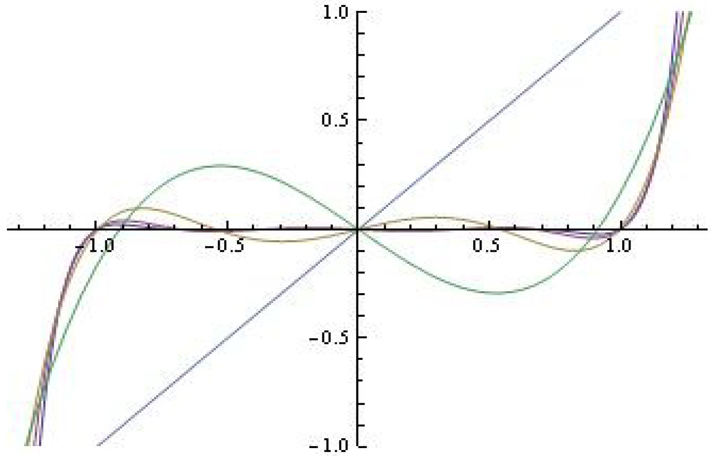
are the polynomials
—see
Figure 1. The level curves are studied. Some applications of the polynomials are also given.
2. Main Results
Let
. Then
Let
(in (1)) coincides with polynomials
. Without going into details, we will note some more interesting level curves.
The level curves
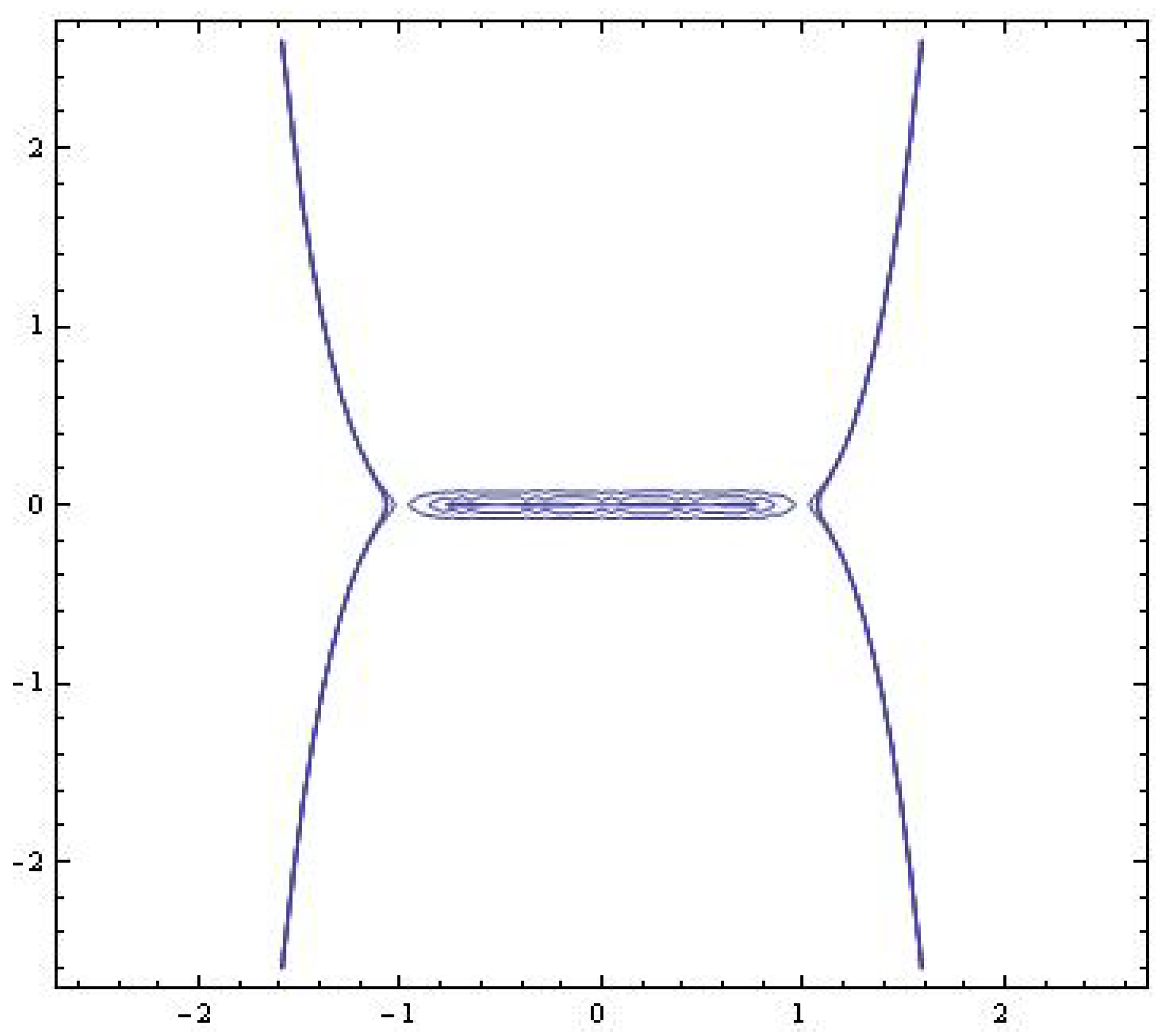
The case (1): .
The Hamiltonian of system (1) (
) is
The level curves
are depicted at
Figure 2.
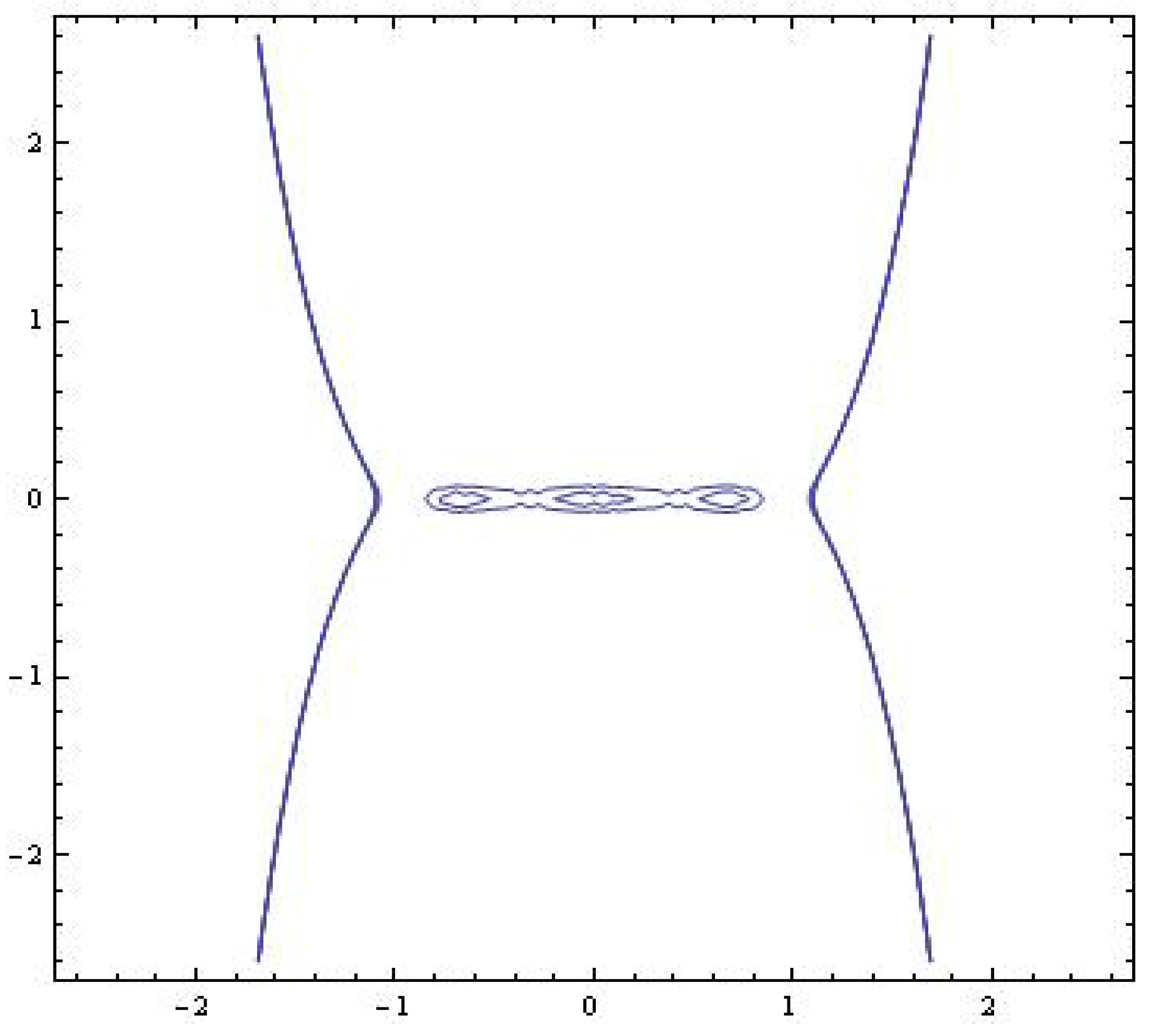
The case (2): .
The Hamiltonian of system (1) (
) is
The level curves
are depicted at
Figure 3.
The model in the light of Melnikov’s considerations
The Melnikov polynomial [
5] for the system
is defined as
It is known [
7,
8] that the system for sufficiently small
has at most
n limit cycles asymptotic to circles of radii
as
if and only if the
nth degree polynomial
has
n positive roots
.
The case .
Consider the model
where
,
.
The following is valid.
Proposition 1. The Lienard–type system for , and for all sufficiently small .
- (a)
for has three hyperbolic limit cycles , and .
- (b)
for has a simple limit cycle and limit cycle with multiplicity two.
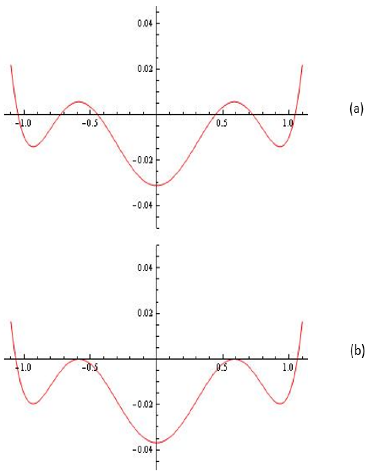
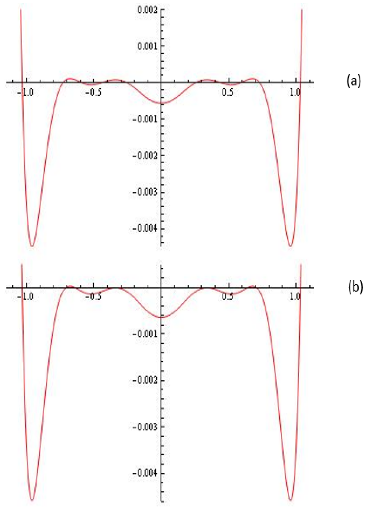
Proof. For the Melnikov polynomial in
(see
Figure 4) we have:
Evidently, for example
we have a simple limit cycle and cycle with multiplicity two. □
The case .
Consider the model
where
,
.
The following is valid.
Proposition 2. The Lienard–type system for , and for all sufficiently small .
- (a)
for has five hyperbolic limit cycles , , 588203, and .
- (b)
for has simple limit cycles , , and limit cycle with multiplicity two.
Proof. For the Melnikov polynomial in
(see
Figure 5) we have:
Evidently, for example
we have three simple limit cycles and limit cycle with multiplicity two. □
Numerical methods for finding zeros of polynomials can be found in [
38,
39,
40].
Some simulations
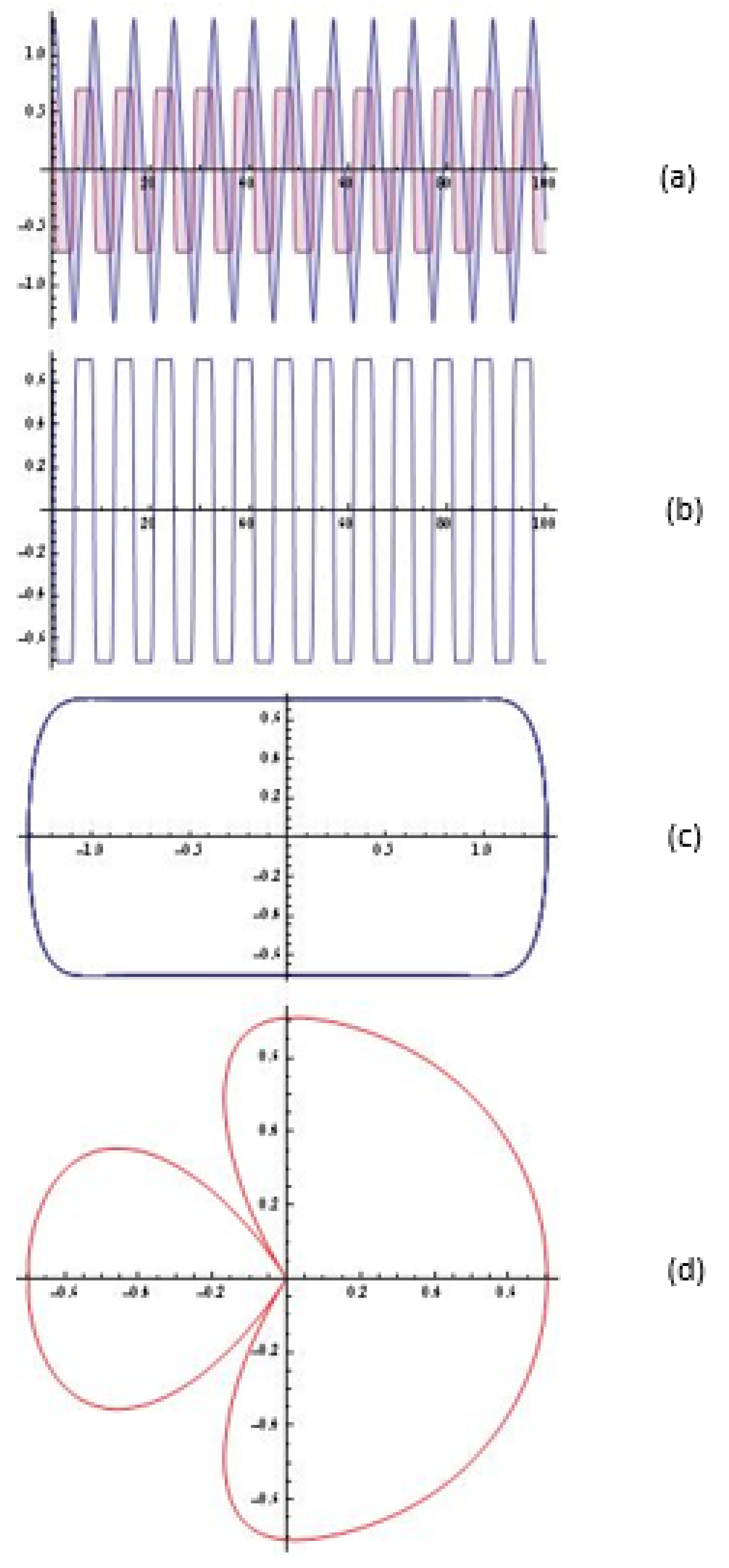
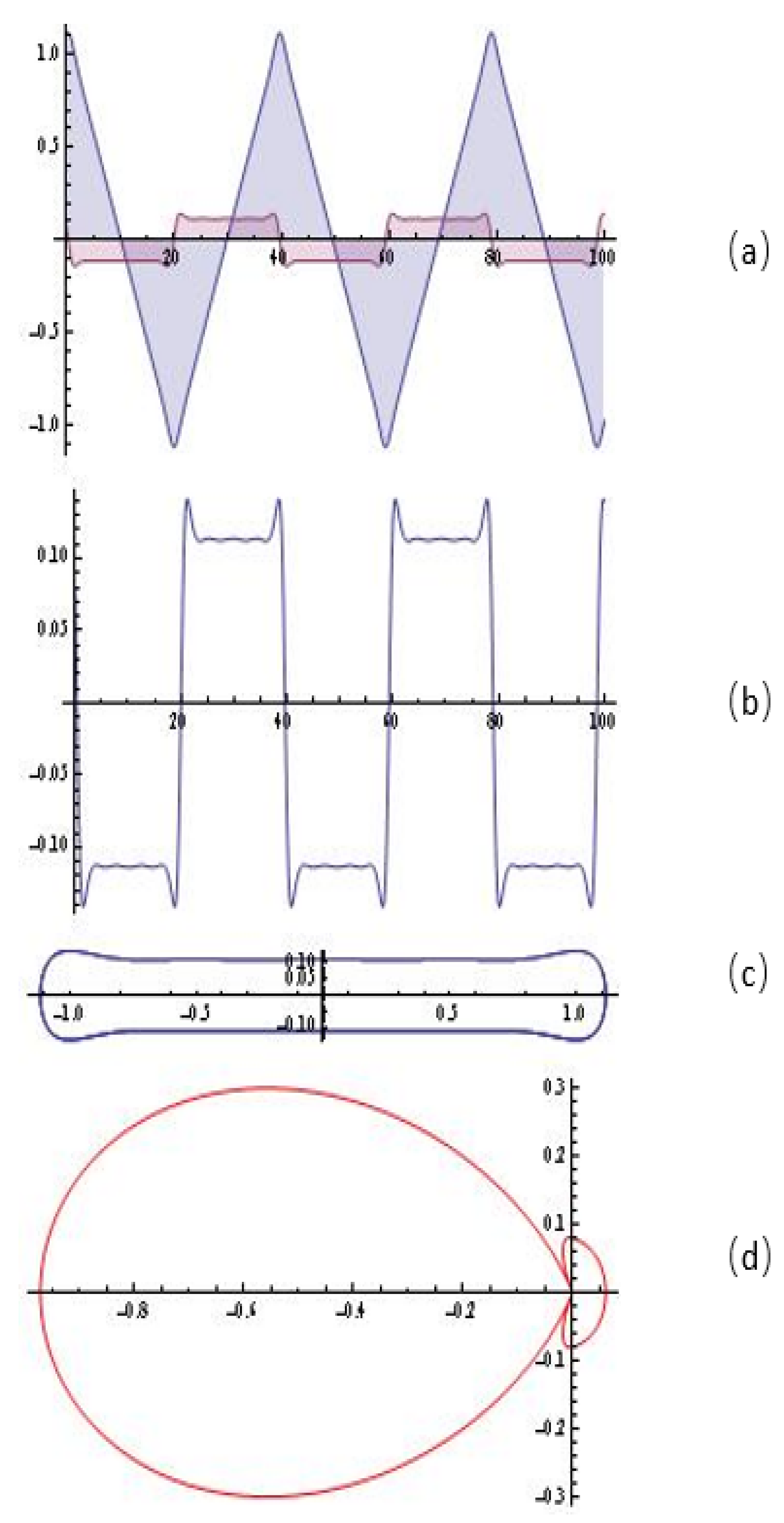
The simulations on the Lienard–type system:
where
- (1)
with , , , ;
- (2)
with , , ,
We will note that some specifics of the amplitudes of these polynomials open up the possibility of modeling signals from the field of antenna-feeder technology.
It is easy to take into account that the change of the variable
t with
(
is the azimuthal angle and
c is the phase difference) in the
-component of the solution of the system (6) leads to radiation diagrams [
41,
42].
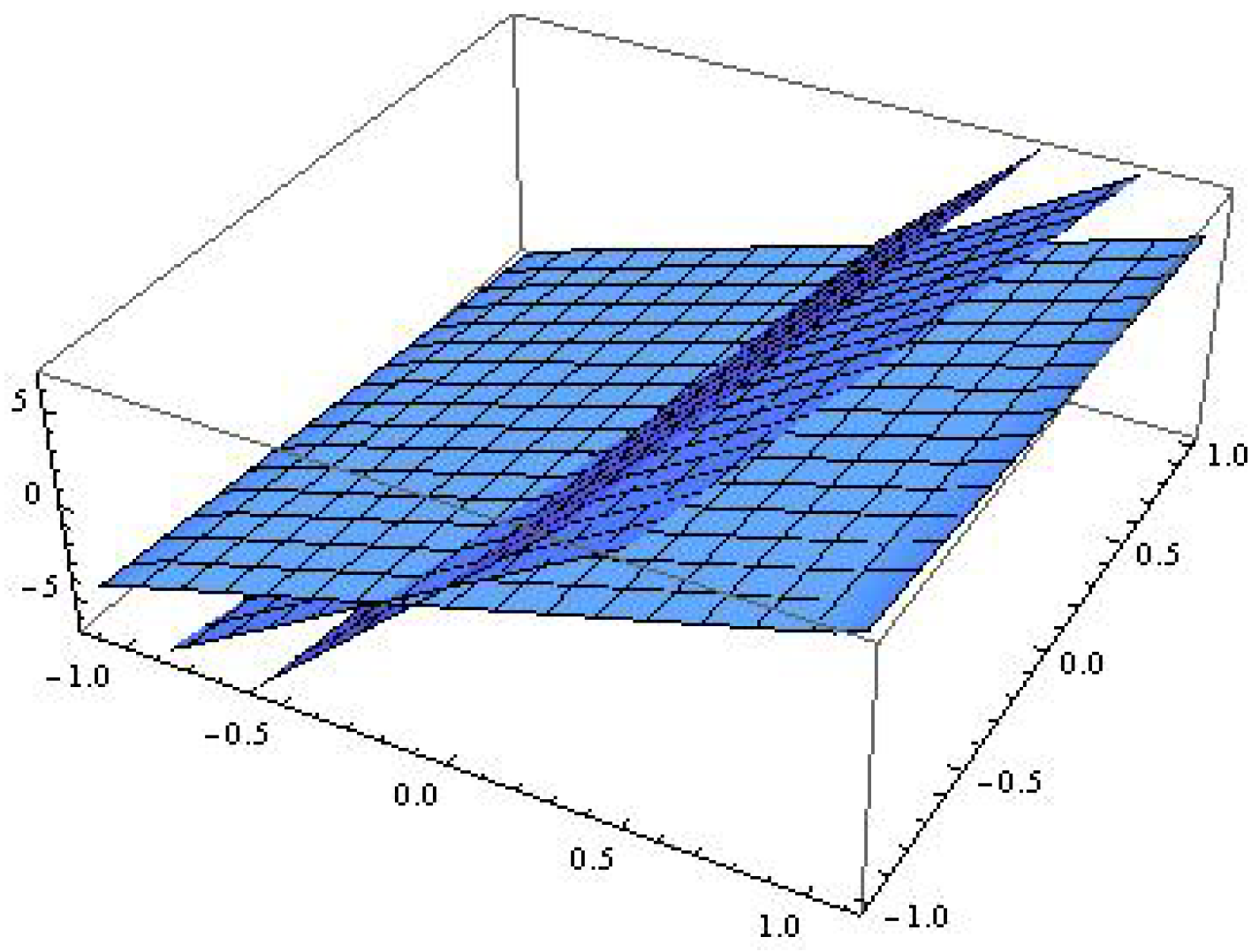
Consider the following model in the light of Zeeman’s approach:
with
and
The catastrophe surfaces
(
) for the model is depicted on
Figure 8.
Consider the model (7) with
and
The catastrophe surfaces
(
) for the model is depicted on
Figure 9.
Associated polynomials—.
We will explicitly note that for modeling specific radiation diagrams, the orthogonal polynomials associated with
—
can also be successfully used, generating from the following recursion [
35]:
The polynomials
for
n = 1,3,5,7,9 and fixed
,
are shown in
Figure 10.
Some simulations
The simulations on the Lienard–type system:
where
with
,
,
,
are depicted on
Figure 11.
All experiments and algorithms were carried out using our own module in CAS Mathematica.
We define the normalized factor as follows
3. Calculator Software Application
We are developing a high-scalable, cloud-based software calculator using serverless architecture [
43]. The serverless architecture enables automatic scaling of the system during high load. Furthermore, it can be used to parallelize suitable computations for higher efficiency. Where possible, we employ various optimization techniques for high-performance calculations, including multi-processor and multi-threading calculations, and hardware intrinsics [
44,
45,
46]. The system is exposing the implemented algorithms using industry-standard application programming interface using HTTP and REST, with data being serialized in JSON and XML formats.
We are developing mobile, native and web-based clients (intellectual property at this stage) to provide an end-user experience for researchers. The following capabilities has been implemented: the user sets: the polynomials (see (1)), which can be arbitrary orthogonal polynomials and their associated polynomials (such as associated Hermite polynomials, associated Gegenbauer polynomials, associated Legendre polynomials, associated Lommel polynomials, q–Lommel polynomials associated with the Jackson q-Bessel function, continuous and bivariate q–Hermite polynomials, extended Gegenbauer polynomials and their q–analogues, associated Jacoby polynomials, Chebyshev and Gegenbauer polynomials of higher kind etc.); the function .
The API can be used by reporting and analytics systems like PowerBI and Excel to further investigate the results [
47].
The application provides an opportunity for research in two directions–the study of the dynamics of differential systems and the generation of special classes of radiation diagrams.
Some of the algorithms used in this paper
- 1.
In the Melnikov polynomials , the coefficients are fractional numbers, and with a high degree of the polynomial, the user is faced with solving a “classic problem with imprecise data”. This requires as a first step the use of an algorithm to approximately find the multiplicities of the zeros of the polynomial, then proceed to an algorithm with a user-fixed rate of convergence to determine all the zeros of the polynomial.
- 2.
Specialized algorithm for detailed Hamiltonian study of system (1) and visualization of “level curves” (assuming implementation of software tools in a user-selected computer-algebraic system for scientific calculations)
- 3.
Algorithm for matching the initial approximations when solving the differential system (1), given its interesting specificity and behavior of the solution in confidential time intervals.
- 4.
Algorithm for control and visualization of the “antenna factor” (with a possibly user-set value of the lateral radiation).
4. Concluding Remarks
Some of our previous research on this issue encouraged us to start developing specialized modules, part of a much more general Web-based application for scientific computing. We mention the above algorithms because some of them are hidden from the user. Determining the number and type of cycles, as we have already mentioned, is a complicated task (with inaccurate data—Algorithm 1). Our proposed module automatically generates theorems in light of Melnikov’s considerations (see e.g., Propositions 1 and 2). This is very important for the user to take further steps in the detailed study of the dynamic model (for example, “level curves”—Algorithm 2) with the corrective corrections set by him in the Lienard differential system of the type of arbitrary high-order orthogonal polynomials or their associated or appropriate classes of Morse-type polynomials, etc. We will explicitly note that the user does not have to be a mathematician! What information about it would be, for example, the standard comment from existing computer algebra platforms: “The solution of the differential system lacks consistency under your chosen set of initial approximations”. After all, we have to provide the user with a satisfactory solution to the task (typical example—the hidden Algorithm 3). Another algorithm hidden from the user is checking the conditions in Lienard’s theorem for the existence of a limit cycle at all! Another example of a hidden algorithm is the recurrent generation of the polynomials under study at a user-fixed degree
n. Algorithm 4 is extremely complex (and at this stage—insufficiently specified and developed). The use of
-the solution component of the corresponding Lienard differential system as an antenna factor is very complicated. As far as the Dolph-Chebyshev technique for synthesis of power pattern end filter prototypes is well known, we note that by analogy we can define hypothetical transmitting functions based on “van Doorn polynomials” (object of consideration in this article). The experts have a word! Of course, research on the “van Doorn array” can be carried out in the light of Soltis considerations [
48], but this is the subject of future development and will be omitted here. We fully understand that the construction of such an ambitious Web-based platform for scientific computing can only be realized with the active participation of specialists from various branches of scientific knowledge.
Author Contributions
Conceptualization, V.K.; methodology, N.K.; software, V.K., A.I. and A.R.; validation, N.K., A.R. and A.I.; formal analysis, N.K. and A.I.; investigation, V.K., A.R. and N.K.; resources, A.I., V.K. and N.K.; data curation, N.K. and V.K.; writing—original draft preparation, V.K., N.K. and A.I.; writing—review and editing, A.R.; visualization, V.K.; supervision, N.K.; project administration, N.K.; and funding acquisition, A.R. and A.I. All authors have read and agreed to the published version of the manuscript.
Funding
This research received no external funding.
Institutional Review Board Statement
Not applicable.
Informed Consent Statement
Not applicable.
Data Availability Statement
Not applicable.
Acknowledgments
This study is financed by the European Union-NextGenerationEU, through the National Recovery and Resilience Plan of the Republic of Bulgaria, project No BG-RRP-2.004-0001-C01. We thank the respected reviewers for their critical comments regarding some components of the proposed web application demo. And that was one of the goals of this article, to get adequate feedback, with a view to future updates and improvements of the planned platform.
Conflicts of Interest
The authors declare no conflict of interest.
References
- Hilbert, D. Mathematical problems (M.Newton Transl.). Bull. Am. Math. Soc. 1901, 8, 437–479. [Google Scholar] [CrossRef]
- Beltrami, E. Mathematics for Dynamic Modeling; Academic Press: Boston, MA, USA, 1987. [Google Scholar]
- Zeeman, E. Catastrophe Theory. Selected Papers 1972–1977; Addison-Wesley: Reading, MA, USA, 1977. [Google Scholar]
- Arnold, V. Geometrical Methods in the Theory of Ordinary Differential Equation; Springer: Berlin/Heidelberg, Germany, 1988. [Google Scholar]
- Melnikov, V.K. On the stability of a center for time–periodic perturbation. Tr. Mosk. Mat. Obs. 1963, 12, 3–52. [Google Scholar]
- Lienard, A. Etude des oscillations entretenues. Revue generale de e’electricite 1828, 23, 901–912, 946–954. [Google Scholar]
- Blows, T.; Perko, L. Bifurcation of limit cycles from centers and separatrix cycles of planar analytic systems. SIAM Rev. 1994, 36, 341–376. [Google Scholar] [CrossRef]
- Perko, L. Differential Equations and Dynamical Systems; Springer: New York, NY, USA, 1991. [Google Scholar]
- Horozov, E.; Iliev, I.D. On the number of limit cycles in perturbations of quadratic Hamiltonian systems. Proc. Lond. Math. Soc. 1994, 69, 198–224. [Google Scholar] [CrossRef]
- Iliev, I.D.; Perko, L.M. Higher order bifurcations of limit cycles. J. Differ. Equ. 1999, 154, 339–363. [Google Scholar] [CrossRef]
- Gavrilov, L.; Iliev, I.D. The limit cycles in a generalized Rayleigh-Lienard oscillator. arXiv 2003, arXiv:2203.02829v1. [Google Scholar] [CrossRef]
- Llibre, J.; Valls, C. Global centers of the generalized polynomial Lienard differential systems. J. Differ. Equ. 2022, 330, 66–80. [Google Scholar] [CrossRef]
- Chen, H.; Lie, Z.; Zhang, R. A sufficient and necessary condition of generalized polynomial Lienard systems with global centers. arXiv 2022, arXiv:2208.06184. [Google Scholar]
- He, H.; Llibre, J.; Xiao, D. Hamiltonian polynomial differential systems with global centers in the plane. Sci. China Math. 2021, 48, 2018. [Google Scholar]
- Smale, S. Mathematical problems for the next century. Math. Intell. 1998, 20, 7–15. [Google Scholar] [CrossRef]
- Zhao, Y.; Liang, Z.; Lu, G. On the global center of polynomial differential systems of degree 2k + 1. In Differential Equations and Control Theory; CRC Press: Boca Raton, FL, USA, 1996; 10 p. [Google Scholar]
- Andronov, A.A.; Leontovich, E.A.; Gordon, I.I.; Maier, A.G.; Gutzwiller, M.C. Qualitative Theory of Second Order Dynamic Systems; Wiley: New York, NY, USA, 1973. [Google Scholar]
- Hale, J.K. Ordinary Differential Equations; Wiley: New York, NY, USA, 1980. [Google Scholar]
- Garcia, I.A. Cyclicity of Nilpotent Centers with Minimum Andreev Number. 2019. Available online: https://repositori.udl.cat/handle/10459.1/67895 (accessed on 1 October 2022).
- Sun, X.; Xi, H. Bifurcation of limit cycles in small perturbation of a class of Lienard systems. Int. J. Bifurc. Chaos 2014, 24, 1450004. [Google Scholar] [CrossRef]
- Asheghi, R.; Bakhshalizadeh, A. On the distribution of limit cycles in a Lienard system with a nilpotent center and a nilpotent saddle. Int. J. Bifurc. Chaos 2016, 26, 1650025. [Google Scholar] [CrossRef]
- Zaghian, A.; Kazemi, R.; Zangenech, H. Bifurcation of limit cycles in a class of Lienard system with a cusp and nilpotent saddle. UPB Sci. Bull. Ser. A 2016, 78, 95–106. [Google Scholar]
- Gaiko, V.; Vuik, C.; Reijm, H. Bifurcation Analysis of Multi–Parameter Lienard Polynomial System. IFAC-PapersOnLine 2018, 51, 144–149. [Google Scholar] [CrossRef]
- Cai, J.; Wei, M.; Zhu, H. Nine limit cycles in a 5-degree polynomials Lienard system. Complexity 2020, 2020, 8584616. [Google Scholar] [CrossRef]
- Xu, W.; Li, C. Limit cycles of some polynomial Lienard system. J. Math. Anal. Appl. 2012, 389, 367–378. [Google Scholar] [CrossRef]
- Xu, W. Limit cycle bifurcations of some polynomial Lienard system with symmetry. Nonlinear Anal. Differ. Equ. 2020, 8, 77–87. [Google Scholar] [CrossRef]
- Hou, J.; Han, M. Melnikov functions for planar near–Hamiltonian systems and Hopf bifurcations. J. Shanghai Norm. Univ. (Nat. Sci.) 2006, 35, 1–10. [Google Scholar]
- Han, M.; Yang, J.; Tarta, A.; Gao, Y. Limit cycles near homoclinic and heteroclinic loops. J. Dyn. Differ. Equ. 2008, 20, 923–947. [Google Scholar] [CrossRef]
- An, Y.; Han, M. On the number of limit cycles near a homoclinic loop with a nilpotent singular point. J. Differ. Equ. 2015, 258, 3194–3247. [Google Scholar] [CrossRef]
- Kyurkchiev, N. The effects on the dynamics of Lienard equation with Morse–type corrections: Level curves. Int. J. Differ. Equ. Appl. 2022, 21, 59–72. [Google Scholar]
- Kyurkchiev, V.; Kyurkchiev, N.; Iliev, A.; Rahnev, A. On Some Extended Oscillator Models: A Technique for Simulating and Studying Their Dynamics; Plovdiv University Press: Plovdiv, Bulgaria, 2022; ISBN 978-619-7663-13-6. [Google Scholar]
- Kyurkchiev, N.; Iliev, A. On the hypothetical oscillator model with second kind Chebyshev’s polynomial–correction: Number and type of limit cycles, simulations and possible applications. Algorithms 2022, 15, 12. [Google Scholar] [CrossRef]
- Kyurkchiev, V.; Iliev, A.; Rahnev, A.; Kyurkchiev, N. Dynamics of the Lienard Polynomial System Using Dickson Polynomials of the (M + 1)-th Kind. The Level Curves. Int. J. Differ. Equ. Appl. 2022, 21, 109–120. [Google Scholar]
- Van Doorn, E. Shell Polynomials and Dual Birth-Death Processes. SIGMA 2016, 12, 49. [Google Scholar] [CrossRef]
- Chihara, T.; Ismail, M. Orthogonal polynomials suggested by a queueing model. Adv. in Appl. Math. 1982, 3, 441–462. [Google Scholar] [CrossRef][Green Version]
- Al-Salam, W. Orthogonal polynomials, Theory and Practice. In NATO ASI Series 294; Neval, P., Ed.; Springer: Dordrecht, The Netherlands, 1990. [Google Scholar]
- Chihara, T. An Introduction to Orthogonal Polynomials; Gordon and Breach Science Publ. Inc.: Philadelphia, PA, USA, 1978. [Google Scholar]
- Kyurkchiev, N.; Andreev, A.; Popov, V. Iterative methods for the computation of all multiple roots of an algebraic polynomial. Annuaire Univ. Sofia Fac. Math. Mech. 1984, 78, 178–185. [Google Scholar]
- Proinov, P.; Vasileva, M. Local and Semilocal Convergence of Nourein’s Iterative Method for Finding All Zeros of a Polynomial Simultaneously. Symmetry 2020, 12, 1801. [Google Scholar] [CrossRef]
- Pavkov, T.M.; Kabadzhov, V.G.; Ivanov, I.K.; Ivanov, S.I. Local Convergence Analysis of a One-Parameter Family of Simultaneous Methods with Applications to Real-World Problems. Algorithms 2023, 16, 103. [Google Scholar] [CrossRef]
- Kyurkchiev, N.; Andreev, A. Approximation and Antenna and Filters Synthesis. Some Moduli in Programming Environment MATHEMATICA; LAP LAMBERT Academic Publishing: Saarbrucken, Germany, 2014; ISBN 978-3-659-53322-8. [Google Scholar]
- Kyurkchiev, N. Some Intrinsic Properties of Tadmor-Tanner Functions: Related Problems and Possible Applications. Mathematics 2020, 8, 1963. [Google Scholar] [CrossRef]
- Rahneva, O.; Pavlov, N. Distributed Systems and Applications in Learning; Plovdiv University Press: Plovdiv, Bulgaria, 2021. [Google Scholar]
- Pavlov, N. Efficient Matrix Multiplication Using Hardware Intrinsics and Parallelism with C#. Int. J. Differ. Equ. Appl. 2021, 20, 217–223. [Google Scholar]
- Duffy, J. Concurrent Programming on Windows; Addison Wesley: Boston, MA, USA, 2009. [Google Scholar]
- Miller, W. Computational Complexity and Numerical Stability. SIAM J. Comput. 1975, 4, 97–107. [Google Scholar] [CrossRef]
- Mateev, M. Creating Modern Data Lake Automated Workloads for Big Environmental Projects. In Proceedings of the 18th Annual International Conference on Information Technology & Computer Science, Athens, Greece, 20–23 May 2024. [Google Scholar]
- Soltis, J.J. New Gegenbauer–like and Jacobi–like polynomials with applications. J. Frankl. Inst. 1993, 33, 635–639. [Google Scholar] [CrossRef]
Figure 1.
The polynomials for fixed ; .
Figure 1.
The polynomials for fixed ; .
Figure 2.
Level curves (the case 1).
Figure 2.
Level curves (the case 1).
Figure 3.
Level curves (the case 2).
Figure 3.
Level curves (the case 2).
Figure 4.
(a) The Melnikov polynomial for and (three limit cycles); (b) The Melnikov polynomial for and (simple limit cycle and limit cycle with multiplicity two).
Figure 4.
(a) The Melnikov polynomial for and (three limit cycles); (b) The Melnikov polynomial for and (simple limit cycle and limit cycle with multiplicity two).
Figure 5.
(a) The Melnikov polynomial for and (five limit cycles); (b) The Melnikov polynomial for and (simple limit cycles , , and limit cycle with multiplicity two).
Figure 5.
(a) The Melnikov polynomial for and (five limit cycles); (b) The Melnikov polynomial for and (simple limit cycles , , and limit cycle with multiplicity two).
Figure 6.
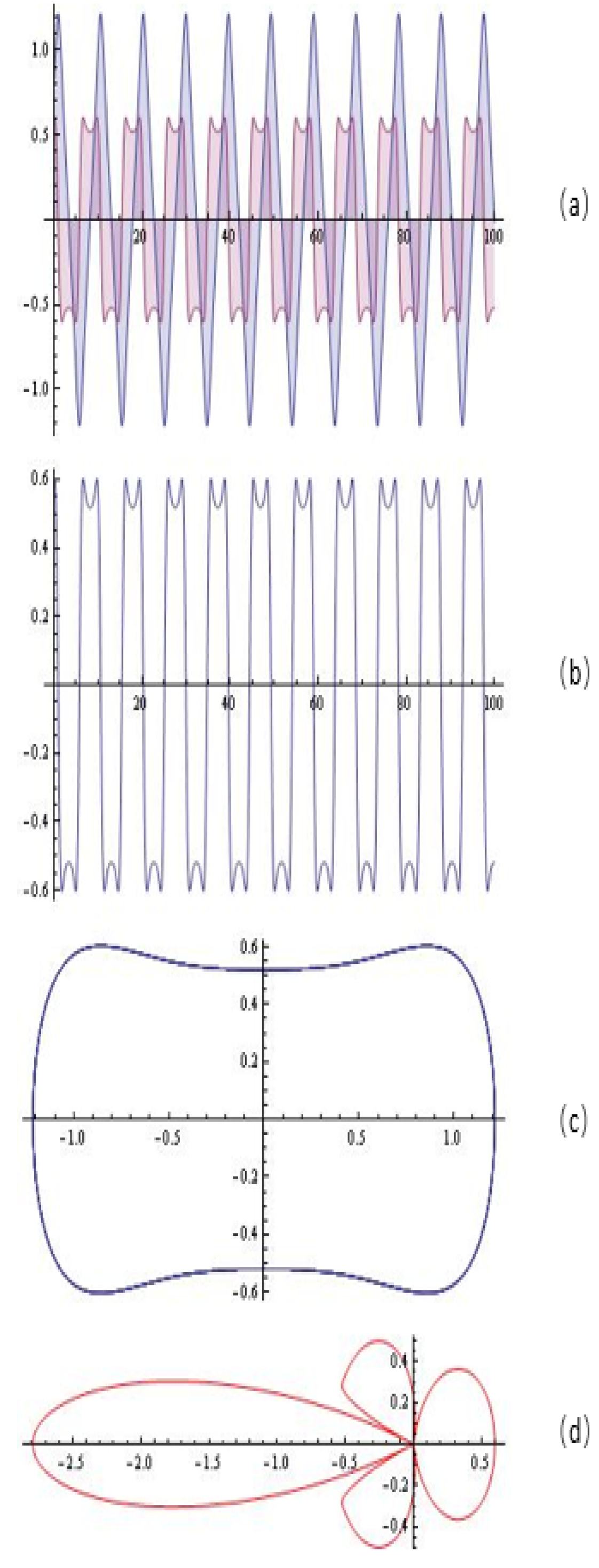
The simulations (system (6)) for , , , ; : (a) the solution of the system; (b) y-component of the solution; (c) the portrait; (d) emitting chart.
Figure 6.
The simulations (system (6)) for , , , ; : (a) the solution of the system; (b) y-component of the solution; (c) the portrait; (d) emitting chart.
Figure 7.
The simulations (system (6)) for , , , ; : (a) the solution of the system; (b) y-component of the solution; (c) the portrait; (d) emitting chart.
Figure 7.
The simulations (system (6)) for , , , ; : (a) the solution of the system; (b) y-component of the solution; (c) the portrait; (d) emitting chart.
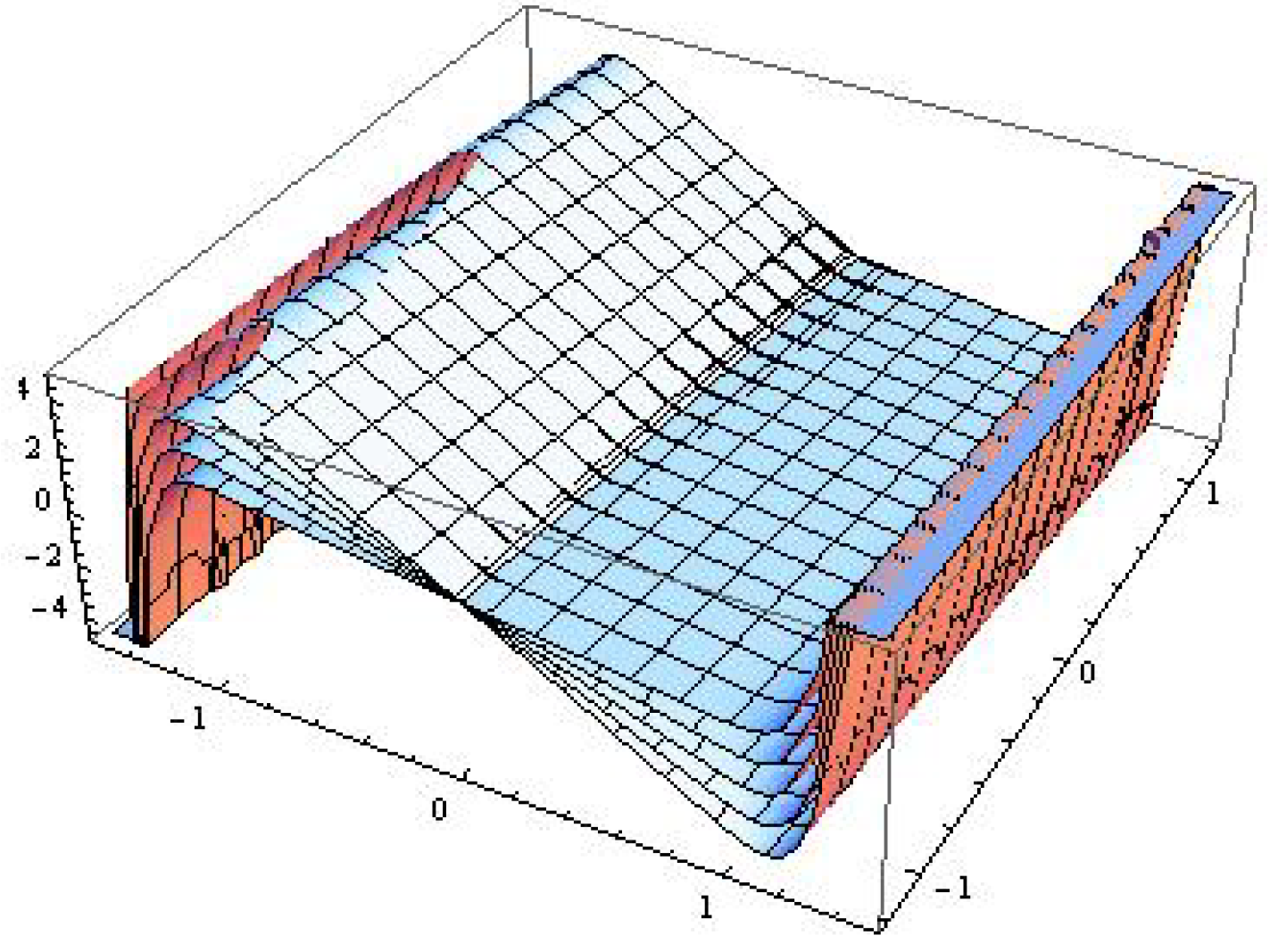
Figure 8.
The catastrophe surfaces in the light of Zeeman considerations.
Figure 8.
The catastrophe surfaces in the light of Zeeman considerations.
Figure 9.
The catastrophe surfaces in the light of Zeeman considerations.
Figure 9.
The catastrophe surfaces in the light of Zeeman considerations.
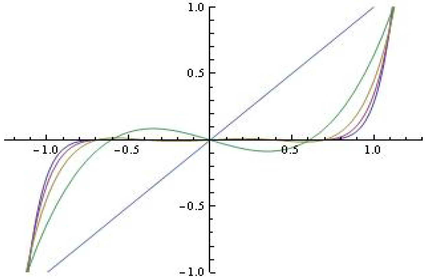
Figure 10.
The polynomials for fixed ; ; .
Figure 10.
The polynomials for fixed ; ; .
Figure 11.
The simulations (system (8)) for , , , ; : (a) the solution of the system; (b) y-component of the solution; (c) the portrait; (d) emitting chart.
Figure 11.
The simulations (system (8)) for , , , ; : (a) the solution of the system; (b) y-component of the solution; (c) the portrait; (d) emitting chart.
| Disclaimer/Publisher’s Note: The statements, opinions and data contained in all publications are solely those of the individual author(s) and contributor(s) and not of MDPI and/or the editor(s). MDPI and/or the editor(s) disclaim responsibility for any injury to people or property resulting from any ideas, methods, instructions or products referred to in the content. |
© 2023 by the authors. Licensee MDPI, Basel, Switzerland. This article is an open access article distributed under the terms and conditions of the Creative Commons Attribution (CC BY) license (https://creativecommons.org/licenses/by/4.0/).


