Noise Cancellation Method Based on TVF-EMD with Bayesian Parameter Optimization

Abstract

To separate the noise and important signal features of the indoor carbon dioxide (CO₂) concentration signal, we proposed a noise cancellation method, based on time-varying, filtering-based empirical mode decomposition (TVF-EMD) with Bayesian optimization (BO). The adaptive parameters of TVF-EMD, that is, bandwidth threshold $\xi$ and B-spline order $n$, were determined by the BO algorithm, and the correlation coefficient for the kurtosis index (CCKur) constituted the objective function. Initially, the objective function CCKur was introduced to systematically identify anomalous signals while preserving signal feature extraction between the modes and the input signal. Subsequently, the proposed signal noise cancellation model based on TVF-EMD and the BO algorithm were employed, along with the Hurst exponent, to extract the sensitive mode. An examination of the optimization indices of the decomposed intrinsic mode functions (IMFs), namely CC, Kur, MI, EE, EEMI, and CCKur, revealed that the synthetic measurement index CCKur and objective function fitness were reasonable and effective. The proposed method exhibited better signal cancellation performance, compared to that of TVF-EMD with the default values, EMD, the moving average method, and the exponential smoothing method.

1. Introduction

Signals contain rich characteristic information; thus, signal processing analysis is crucial in the development of natural sciences, particularly in environmental monitoring [1]. There is a relationship between the indoor carbon dioxide concentration and respiratory mucosal symptoms [2,3]; hence, it is essential to monitor and study carbon dioxide concentrations in various functional building spaces in real time. However, when there are sudden changes in background concentrations of CO₂ or equipment sampling failures, the CO₂-monitoring signal becomes noisy, making it difficult to distinguish important signal features from noise. Therefore, the noise cancellation of the CO₂-monitoring signal is important.

There are various methods of signal denoising, and the most commonly used include smoothing, Fourier transform [4], wavelet theory [5], and Hilbert–Huang transform [6,7]. Smoothing is a simple and convenient method that denoises the signal at the expense of reduced temporal resolution [8,9]. In Fourier and wavelet transforms, the selection of the a priori basis function directly affects the results of signal noise reduction [9,10], which is a major limitation in the application of these methods. The core of the Hilbert–Huang transform is empirical modal decomposition (EMD). The EMD model identifies the intrinsic oscillatory modes in the signal, based on the local characteristic timescale of the signal, and, accordingly, decomposes the raw signal into several intrinsic mode functions (IMFs) without requiring previous knowledge of original signal values [11]. Therefore, EMD is commonly adopted for analyzing adaptive, nonlinear, and nonstationary signal processing, such as indoor CO₂ concentration signals. However, the EMD methods applied for noise reduction are subject to modal aliasing and endpoint effects, known as the mode-mixing issue [12]. In other words, EMD is prone to noise. Based on the framework of EMD, the improved methods, such as ensemble EMD [13] and noise-assisted MEMD [14], are proposed to solve the intermittence problem of EMD. However, there are still many problems with these methods, such as unselectable parameters of noise and failure to separate modes.

The time-varying, filtering-based empirical mode decomposition (TVF-EMD) was developed to address the shortcomings of the EMD model, with the shifting process completed by the B-spline approximation filter [12]. The three main features of TVF-EMD, compared with most existing methods, can be summarized as follows: (1) The TVF-EMD method can simultaneously address the issues of separation and intermittence [15]. (2) With a B-spline approximation filter integrated into the shifting process, TVF-EMD solves the issue of mode mixing and maintains time-varying features. (3) The enhanced stopping criterion improves the performance of the TVF-EMD model for low sampling rates. However, two significant effects, bandwidth threshold $\xi$ and B-spline order $n$, have direct impacts on the separation and filter performance of the time-varying filter, respectively [12]. A reasonable selection of a combination of the two parameters in advance enables the TVF-EMD model to resolve the mode-mixing problem, thereby achieving optimal noise reduction. Hence, the choice of parameters for the TVF-EMD is clearly important.

Many optimization methods are used in hyperparameter estimation. Among the most widely used are the grid search [16,17], random search [18], Genetic algorithm [19], and Bayesian optimization (BO) algorithms [20,21]. Unlike grid and random searches, the framework of BO leverages information from existing data, and the current search for optimal values is based on previous search results [22]. In addition, there are swarm intelligence optimization technologies that imitate the behaviors of various organisms, such as ants [23], particle swarm optimization [24], fish schools [25], glow worm swarm optimization [26], and grey wolves [27], to achieve optimal parameter estimation. Zhou et al. [28] proposed the parameter-adaptive TVF-EMD feature extraction method, based on improved GOA, to deal with the mechanical fault diagnosis. However, the Genetic algorithm and the swarm intelligence optimization algorithm can be categorized as population optimization algorithms. Population optimization algorithms are not particularly suitable for model hyperparameter tuning because they require a sufficient number of initial sample points and are not particularly efficient for optimization. To accelerate computation, Bayesian hyperparameter optimization based on surrogate algorithms is widely used. The tree-structured Parzen estimator (TPE) is one of the most notable hyperparameter optimization methods [29,30]. The Parzen-based estimator can naturally handle complex search spaces and can be extended to dozens of variables, with at least a thousand observations [31]. Therefore, selecting a BO algorithm based on a tree-structured Parzen estimator (BO-TPE) is a reasonably effective method for TVF-EMD parameters.

In the aforementioned denoising theories, the smoothing method can reduce the signal resolution in time. Indoor CO₂ concentrations in buildings is a typical non-stationary signal. These signal-denoising methods, such as Fourier transform, EMD, ensemble EMD, and noise-assisted MEMD, are not suitable for processing non-stationary signals. The wavelet transform is suitable for dealing with non-stationary, time-varying signals, but there is the problem of difficult wavelet basis selection. The TVF-EMD method can solve the shortcomings of the above methods. Combined with the hyperparameter algorithm, the TVF-EMD method can match the appropriate parameters more quickly to achieve accurate noise reduction of the indoor CO₂ concentration.

Considering this background, this study proposed an optimized TVF-EMD method, based on the BO-TPE algorithm, for noise cancellation. First, the correlation coefficient was defined as a comprehensive index for the objective condition of TVF-EMD parameter optimization. In addition, the correlation coefficient was used as the mode selection criterion for the target IMF. Second, an optimization algorithm called BO-TPE was used to search for the optimal combination of TVF-EMD parameters to match the input signal. The effectiveness of the proposed method was suitable for processing the noise of the non-stationary signal, especially large amplitudes, but with dispersed distribution noise signals. The noise reduction results of the CO₂ concentration signals from two different sets of functional building spaces demonstrated that the method was successful in canceling noise and could be effective in CO₂-monitoring engineering applications.

2. Preliminaries

2.1. Time-Varying Filter Empirical Mode Decomposition

EMD can decompose a given signal $x\left(t\right)$ into a set of component signals known as IMFs and residual $r\left(t\right)$, as shown in the following equation:

$$x\left(t\right)={\displaystyle \sum _{i=1}^{N}im{f}_i\left(t\right)+r\left(t\right)}$$

(1)

where $im{f}_i\left(t\right)$ represents the $\mathrm{i}$-th IMF. The screening process of EMD comprises two steps: (1) estimation of the “local mean” $m\left(t\right)$ and (2) recursive subtraction of the $m\left(t\right)$ from the input signal until the resulting signal meets the stopping criterion.

In TVF-EMD, the mono-components are replaced by local narrow-band signals to improve the performance of the EMD method. These signals have properties similar to those of the IMF but provide a meaningful Hilbert spectrum. The local instantaneous bandwidth is used to define local narrow-band signals, which necessitate that the bandwidth be below a given threshold value. This method aims to initially determine the local cut-off frequency and subsequently applies a time-varying filter. The TVF-EMD shifting process is performed using a time-varying filter, which primarily involves three main steps [12]:

• Local cutoff frequency rearrangement

Step 1: Locate the maximum time consumption of $x\left(t\right)$, expressed as $u_i,i=1,2,3\dots$

Step 2: Determine all intermittences, expressed as $e_j,\mathrm{where} j=1,2,3\dots$ by setting a threshold value for the rate of change within a certain time span. These breaks should satisfy the following condition:

$$\frac{\max \left({\varphi }_{bis}^{\prime }(u_i:u_{i+1})\right)-\min \left({\varphi }_{bis}^{\prime }(u_i:u_{i+1})\right)}{\min \left({\varphi }_{bis}^{\prime }(u_i:u_{i+1})\right)}>\rho$$

(2)

where $\rho =0.25$, and ${\varphi }_{bis}^{\prime }$ is the bisection frequency.

Step 3: The condition of the rising edge of ${\varphi }_{bis}^{\prime }\left(e_j:e_{j+1}\right)$ is ${\varphi }_{bis}^{\prime }\left(u_{i+1}\right)-{\varphi }_{bis}^{\prime }\left(u_i\right)>0$, and ${\varphi }_{bis}^{\prime }\left(e_j:e_{j+1}\right)$ is considered the floor. Similarly, the falling edge is ${\varphi }_{bis}^{\prime }\left(u_{i+1}\right)-{\varphi }_{bis}^{\prime }\left(u_i\right)<0$, and ${\varphi }_{bis}^{\prime }\left(e_{j+1}:e_j\right)$ is considered the floor. The rest of ${\varphi }_{bis}^{\prime }$ refers to the peak.

Step 4: By interpolating between the peaks, the final local cutoff frequency can be obtained. During the local cutoff frequency rearrangement phase, the TVF-EMD addresses the separation and intermittence problems.

2.

Shifting process for TVF-EMD

Step 1: Address the local cut-off frequency for signal $x\left(t\right)$.

Step 2: Filter the input signal $x\left(t\right)$ using the time-varying filter (i.e., B-spline approximation filter) to obtain the local mean. The bandwidth threshold $\xi$ determines the separation effect and whether the input signal must be filtered. The B-spline order $n$ is independent of the cutoff frequency estimate, which determines the attenuation and filtering effect of the TVF.

Step 3: Verify that the residual signal satisfies the condition of the stopping criterion indicated below:

$$\theta \left(t\right)=\frac{B_{Loughlin}\left(t\right)}{{\phi }_{avg}\left(t\right)}$$

(3)

where $B_{Loughlin}$ is the Loughlin instantaneous bandwidth, and ${\phi }_{avg}\left(t\right)$ is the weighted average instantaneous frequency. The detailed calculation process of TVF-EMD was discussed in previous studies [12,32].

2.2. Bayesian Optimization

The BO-TPE works by assuming that the black-box function is sampled from a Gaussian mixture model and maintains the posterior distribution of that function while making observations. The posterior probabilities are updated using new sample points at each iteration. To prevent the results from falling into local optima, the BO algorithm adds a stochastic algorithm to balance stochastic exploration and posterior distribution.

The probabilistic surrogate model and acquisition function are the core components of the BO method, and the TPE is the probabilistic surrogate model of the study. The BO algorithm is highly efficient for hyperparameter estimation, as it exhibits excellent convergence.

The objective of Bayesian optimization is to determine the global maximum or minimum value of the objective function in the hyperparameter space. This study aimed to determine the maximum value of the true fitness objective function on a bounded set $\chi$ in a limited number of iterations. The mathematical model of the BO algorithm is as follows:

$$x^{\ast }=\arg {\max }_{x\in \chi } f\left(x\right)$$

(4)

where the point $x^{\ast }$ that maximizes the surrogate function is the proposed point for evaluating the objective function $f\left(x\right)$.

Let us suppose that the observation values are of the form $D_{1:t}={\left\{x_i,y_i\right\}}_{i=1}^t$, where $y_i$ is the generalization accuracy of the algorithm under $x_i$. This can be considered the generalization accuracy of random observations $y=f\left(x\right)+\epsilon$, where the noise introduced into the observation $\epsilon$ is assumed to satisfy $\epsilon ~N\left(0,{\sigma }_{\epsilon }^2\right)$. To explore $x^{\ast }$ in the hyperparameter space, the acquisition functions were obtained, in which the maximum of the function was calculated as

$$x_{t+1}=\arg \max x_t\left(x,D\right)$$

(5)

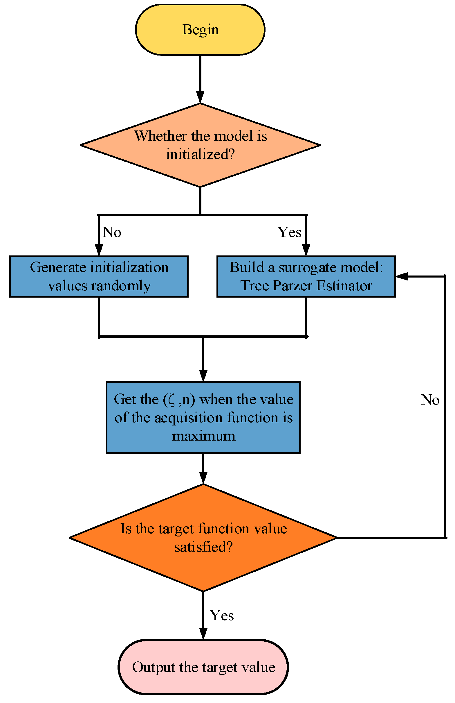
In this study, the bandwidth threshold $\xi$ and B-spline order $n$ were the independent variables $x$ of the BO model, and the flowchart of the Bayesian optimization was outlined as follows (see Figure 1). First, we determined whether the parameters of the model, $\xi$ and $n$, were initialized, and if not, the initial parameters were generated randomly. If the parameters were initialized, the values were brought into the tree Parzer estimator surrogate model. Subsequently, it was judged whether the acquisition function reached its maximum value when given $\xi$ and $n$. If the maximum value of the target function was satisfied, the value of the two parameters were output. If not, the values of the surrogate model parameters were updated until the requirements were met.

3. Adopted Methodology

The proposed optimized TVF-EMD method is based on the BO-TPE algorithm. It aims to search for optical combinations of parameters for the bandwidth threshold $\xi$ and B-spline order $n$ using the objective function, which determines the merits of the decomposition results. The kurtosis index $Kur$ depends on the distribution density of the signal, which is highly sensitive to large amplitudes with dispersed distributions. A kurtosis index value between 0 and 3 indicates that the center peak of the signal is lower and broader, compared to the normal distribution represented by $Kur=3(Kur\approx 3)$. In contrast, $Kur>3$ indicates that the central peak of the signal is higher and sharper. Thus, a smaller kurtosis index is required for a more sensitive identification of outliers. However, to avoid excessive noise cancellation, the correlation coefficient (CC) is used to characterize the similarities between original and decomposing signals. Therefore, the synthetic measurement index, consisting of the kurtosis index and CC, was developed as an objective function for TVF-EMD parameter optimization. The synthetic measurement index, correlation coefficient for kurtosis index (CCKur), was calculated as follows:

$$CCKur=\frac{\left|CC\right|}{Kur}$$

(6)

$$CC:{\rho }_{x,imf}=\frac{{\displaystyle \sum _{i=1}^N\left(x_i-\overline{x}\right)\left(im{f}_i-\overline{imf}\right)}}{\sqrt{{\displaystyle \sum _{i=1}^N{\left(x_i-\overline{x}\right)}^2{\left(im{f}_i-\overline{imf}\right)}^2}}}$$

(7)

$$Kur={\frac{1}{M}{\displaystyle \sum _{m=0}^{m-1}{x}^4\left(m\right)}/\left(\frac{1}{M}{\displaystyle \sum _{m=0}^{m-1}{x}^4\left(m\right)}\right)}^2$$

(8)

As the original BO algorithm was developed to determine the maximum value, the method used the maximum CCKur between the original signal and the modes obtained by TVF-EMD as the fitness. Therefore, the maximization of CCKur was the optimization problem expressed below:

$$\{\begin{array}{c}fitness=\underset{\gamma \in \left\{\xi ,n\right\}}{\max }\left\{CCKur\right\}\\ \begin{array}{c}\xi \in \left(0,0.4\right]\\ n\in \left[1,16\right]\end{array}\end{array}$$

(9)

where $fitness$ is the objective function, and $\gamma =\left\{\xi ,n\right\}$ represents the parameter combination of the TVF-EMD method to be optimized. The CC of the original signal $x\left(t\right)$, which is a function of mode $imf\left(t\right)$ with the same length as $N$, is described in Equation (7).

Ensuring the reliability of the parameter optimization was essential, and the number of modes after CO₂ signal decomposition must be at least two. After several attempts, it was discovered that the bandwidth threshold $\xi$ met $0\le \xi \le 0.4$, and $1\le n\le 16$ satisfied the requirements. The same number of modes was obtained with the typically used standard EMD, and the maximum number of modes for the TVF-EMD was set to $K={\log }_{2}N$ [4].

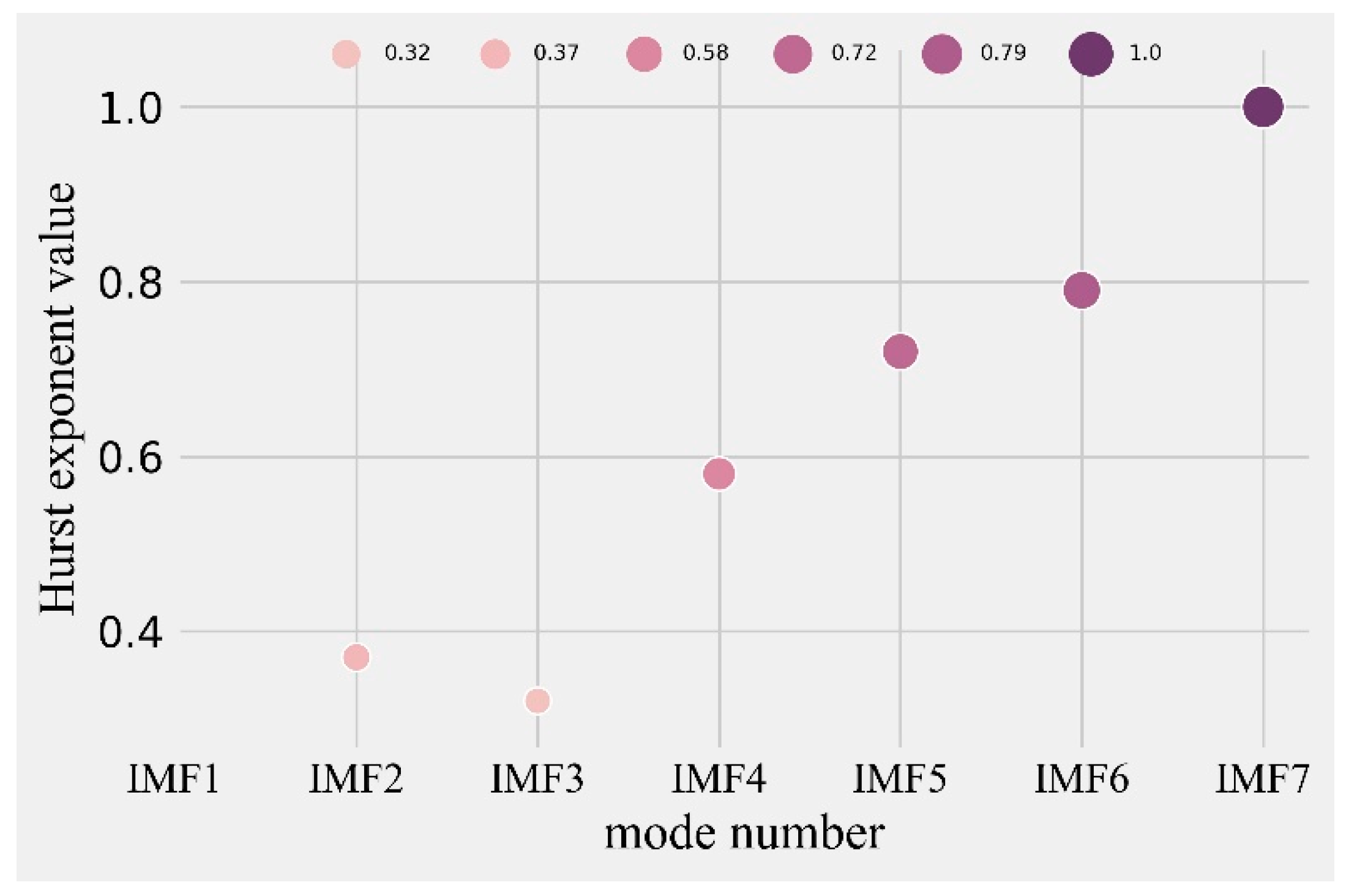
The autocorrelation properties of the signal and Hurst exponent $H$ were evaluated to distinguish noise from the most relevant modes. When $0\le H<0.5$, two signals were anticorrelated. In contrast, $H=0.5$ indicated white noise, and $H>0.5$ represented a positive correlation. In this study, the threshold for the Hurst index was defined as 0.5 ($H_{thr}=0.5$). The detailed steps of the noise cancellation methodology were as follows:

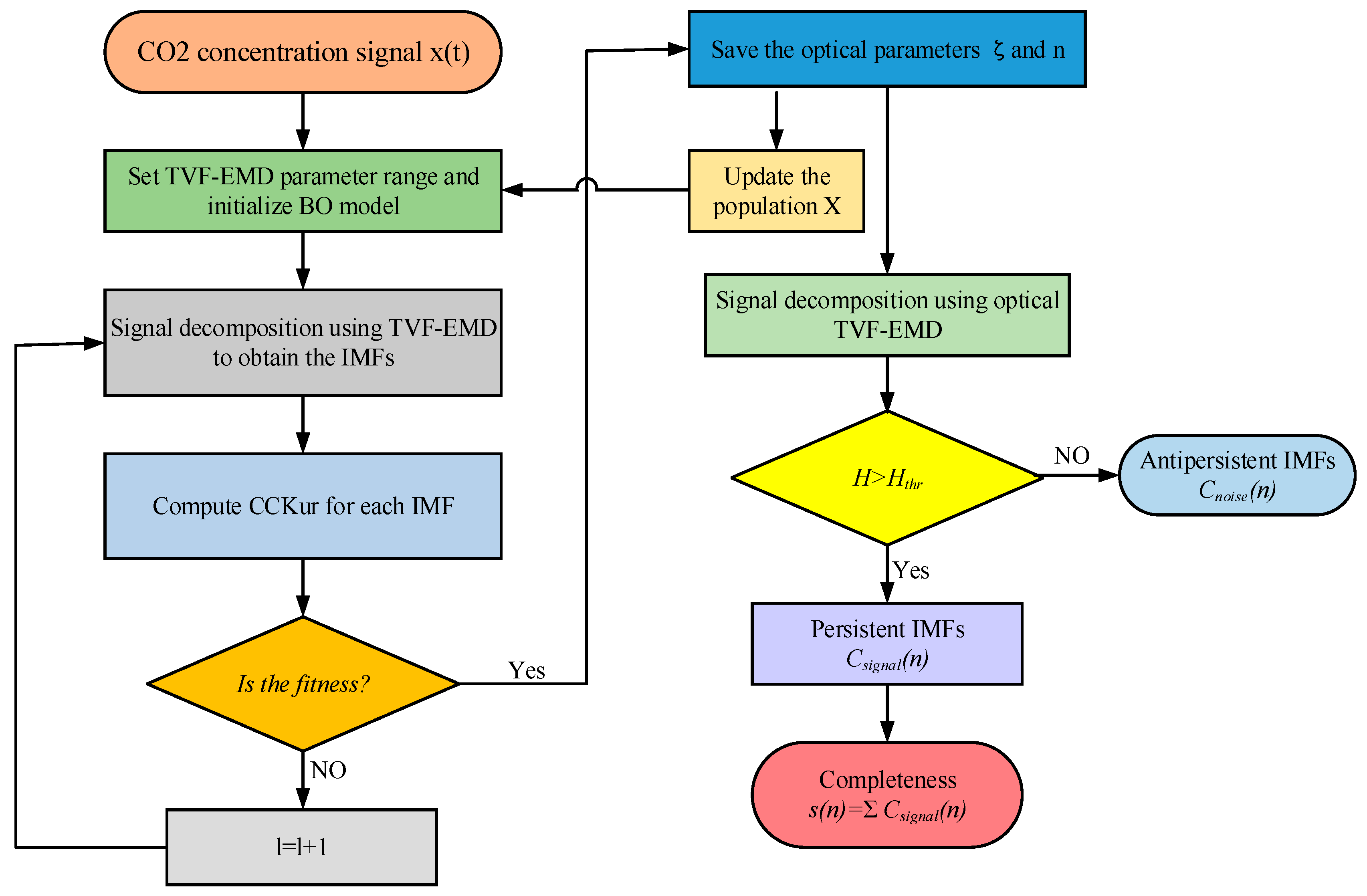
Step 1: Input the CO₂ concentration signal $x\left(t\right)$ and set the parameter population $X$ to the TVF-EMD model. Concurrently, initialize the parameters of BO algorithms and population $X$, including the bandwidth threshold $\xi$ and B-spline order $n$.

Step 2: Decompose the signal $x\left(t\right)$ using the TVF-EMD model for the parameter combination of $\xi$ and $n$, and then calculate the IMFS to obtain the objective function $fitness$, where the best fitness for each iteration of the BO algorithm is stored.

Step 3: If the stored value of fitness satisfies the threshold, then save the optical parameters $\xi$ and $n$. Otherwise, $l=l+1$, and continue Step 2 to update parameters $\xi$ and $n$ until the maximization of $CCKur$ is up to requirements.

Step 4: Obtain and save the best maximization of $CCKur$ and the corresponding parameter combination of the TVF-EMD.

Step 5: Update the population $X$ by obtaining the best parameter combination.

Step 6: Use the optimized TVF-EMD with the combination parameters $\xi$ and $n$ to decompose the original CO₂ signal.

Step 7: Calculate the Hurst exponent $H$ of each IMF. If the $H$ is greater than $H_{thr}$, save the sensitive IMF.

Step 8: Sum these sensitive IMFs together to obtain the reconstructed signals. The other insensitive IMFs are considered to be noise.

A flowchart of the proposed BO-based TVF-EMD method for the SNC model is shown in Figure 2.

4. Results and Discussion

4.1. Data Acquisition

The CO₂ concentration was analyzed after denoising the CO₂ signals, which were obtained using pump-activated CO₂ concentration detectors installed in offices and university classrooms. The CO₂ signals were sampled at a frequency of 5 s and monitored continuously for 24 h. Figure 3 illustrates the CO₂ signal from an $8\mathrm{m}\times 8\mathrm{m}\times 3\mathrm{m}$ regular-sized office accommodating approximately six to ten people. The detector measured the CO₂ concentration at a height of 2.8 m in the room. The specifications used are listed in

Table 1. Specifications considered for processing CO₂ signals.

Parameters	Value
Sampling frequency	5 s
Measurement accuracy	1 ppm
Error range	5%
Time sample length	24 h

.

4.2. Analysis of the Simulated Signal

4.2.1. Simulation and Comparison

The result of the signal decomposition using the EMD method is shown in Figure 4a. Signal $x\left(t\right)$ was decomposed into nine IMFs. Therefore, the maximum number of modes for TVF-EMD was set to three. The original CO₂ signal was then processed by the proposed TVF-EMD model, based on the BO algorithm. The combination of the bandwidth threshold $\xi$, B-spline order $n$, and the maximum $CCKur$ of the BO algorithm were $\xi =0.31$, $n=7$, and $CCKu{r}_{max}=0.49$, respectively. Figure 4b shows the signal decomposition results obtained using the optimized TVF-EMD model.

The Hurst exponent was computed for each IMF. As shown in Figure 5, the different values of the Hurst exponent for the seven consecutive IMFs were NaN, 0.37, 0.32, 0.58, 0.72, 0.79, and 1.0, respectively. The first IMF, second IMF, and third IMF had a Hurst exponent value of less than the threshold of 0.5, indicating the weak long-range autocorrelation of residual signals. The fourth through seventh IMFs were reserved for further processing and summed to obtain the noise-reduced signal. To better illustrate the effects of signal noise cancellation by the proposed method, a quantitative comparison of the three denoising methods was conducted, as shown in Figure 6. Conventional noise reduction methods, such as exponential smoothing and the moving average method, were not highly effective in eliminating the impact of shock signals. This comparison verified the superiority of the TVF-EMD method in signal noise cancellation.

4.2.2. The Effects of TVF-EMD Parameters

In addition to $CC$ and $Kur$, other indices, including mutual information (MI) [33], energy entropy (EE) [34], and energy entropy mutual information (EEMI) [28], are commonly used to evaluate the degree of optimization in signal processing. As shown in Figure 7, the selection of optical parameters $\xi$ and $n$ did not significantly change the MI, EE, and EEMI indices of IMF1 to IMF7, indicating that these indices were insensitive to the optical parameters. In contrast, $CC$, $Kur$, and $CCKur$ were sensitive to optical parameters.

Different parameters affected the decomposition results to different degrees. The decomposition of the CO₂ concentration signal $x\left(t\right)$ and the effect of TVF-EMD parameters on the decomposition results are shown in Figure 8. The bandwidth threshold $\xi$ reached 0.95 in the decomposition results, indicating that the selection of the optimization index should be sensitive to the change in $\xi$. Therefore, we analyzed the results of CC, Kur, MI, EE, EEMI, and $CCKur$ under varying $\xi$. As shown in Figure 9, when $\xi$ assumed values of 0.1, 0.2, and 0.31 (the optimal parameter), eight, nine, and seven IMFs were obtained by decomposition, respectively. When $\xi$ was at least four, two IMFs were obtained, indicating that mode aliasing and under-decomposition occurred. When $\xi$ increased from 0.1 to 0.31, the MI, EE, and EEMI indices of the IMFs did not change significantly, suggesting that these indices were insensitive to the variation in $\xi$. The CC, Kur, and $CCKur$ indices were sensitive to $\xi$; hence, they can be selected as indices for the best parameters. When $\xi =0.31$, the sum of the $CCKur$ indices of IMF1 to IMF9 was the largest, which indicates that $CCKur$ can be regarded as the best optimization model. The results showed that (1) $\xi$ had to be at least 4 for mode aliasing and under-decomposition to occur; (2) $CC$, $Kur$, and $CCKur$ indices were sensitive to $\xi$, whereas MI, EE, and EEMI indices were not; (3) the proposed $CCKur$ index and objective function $\underset{\gamma \in \left\{\xi ,n\right\}}{\max }\left\{CCKur\right\}$ were effective; and (4) the value of 0.31 for $\xi$ was reasonable and correct.

4.3. Validation of the Proposed Method

To study the denoised signal performance of the proposed signal cancellation method, the signal-to-noise ratio (SNR), mean squared error (MSE), relative squared error (RSE), and normalized root mean squared error (NRMSE) were used to evaluate the quality of the reconstructed signals. The SNR is the ratio of the original signal power to noise signal power. The MSE calculates the error by squaring the difference between the reconstructed and original signals and averaging all values. The RSE is the ratio of the MSE to the square of the difference between the original signal and the mean of the original signal. The smaller the values of MSE, RSE, and NRMSE, the better the noise reduction effect. In contrast, a smaller SNR implies a poor noise reduction effect. The following equations were used for the comparisons (Equations (10)–(13)).

$$SNR\left(\mathrm{db}\right)=10\log \left(\frac{P_s}{P_n}\right)$$

(10)

$$MSE=\frac{1}{N}{\displaystyle {\sum }_{n=1}^N{\left(x\left(n\right)-\widehat{x}\left(n\right)\right)}^2}$$

(11)

$$RSE=\frac{{\displaystyle {\sum }_{n=1}^N{\left(\widehat{x}\left(n\right)-x\left(n\right)\right)}^2}}{{\displaystyle {\sum }_{n=1}^N{\left(\overline{x}\left(n\right)-x\left(n\right)\right)}^2}}$$

(12)

$$NRMSE=\frac{\sqrt{\frac{1}{N}{\displaystyle {\sum }_{n=1}^N{\left(x\left(n\right)-\widehat{x}\left(n\right)\right)}^2}}}{x_{\max }-x_{\min }}$$

(13)

where $P_s$ and $P_n$ represent the effective powers representing the signal and noise, respectively. Here, $x\left(n\right)$, $\widehat{x}\left(n\right)$, and $\overline{x}\left(n\right)$ denote the original signal, reconstructed signal, and the average of the original signal, respectively.

A detailed study was conducted, and signal cancellation performance was evaluated for different denoising methods in terms of SNR, MSE, RSE, and NRMSE. The CO₂ signals studied from the university classroom had a capacity of 100 students. As shown in

Table 2. Comparison of the noise reduction effect under different signal-denoising models.

Index	Proposed TVF-EMD $(\mathit{\xi }=0.015,\mathit{n}=4)$	TVF-EMD with Default Values $(\mathit{\xi }=0.1,\mathit{n}=26)$	EMD	Moving Average (Window = 40)	Exponential Smoothing $(\mathit{\alpha }=0.5)$
SNRabs	71.376	71.296	71.141	71.251	71.239
MSE	7.877	95.976	3217.423	154.281	21.473
RSE	0.000276	0.00336	0.112	0.00540	0.000752
NRMSE	0.0166	0.0581	0.3614	0.0736	0.0274

, the proposed noise cancellation model yielded the largest absolute SNR value. The MSE, RES, and NRMSE of the proposed method were all smaller than those obtained by the TVF-EMD, EMD, moving average, and exponential smoothing methods, indicating that the proposed noise cancellation model had superior noise reduction quality for the CO₂ concentration signal.

5. Conclusions

An optimized TVF-EMD model based on a Bayesian algorithm was adopted to develop a noise cancellation model for denoising the CO₂ concentration signal of a building. The Bayesian algorithm was used to optimally estimate the TVF-EMD parameters, namely the bandwidth threshold $\xi$ and B-spline order $n$, and the adaptive matching of the given CO₂ concentration signal. The main conclusions can be summarized as follows:

In parameter optimization, a synthetic measurement index consisting of CCKur was used as the objective function of TVF-EMD. This function could identify anomalous signals while preserving the signal profile and avoided excessive noise reduction. In the proposed noise cancellation model, a thresholding parameter $H_{thr}=0.5$, based on the Hurst exponent, was introduced as a measurement index for selecting the relevant IMFs for signal reconstruction.

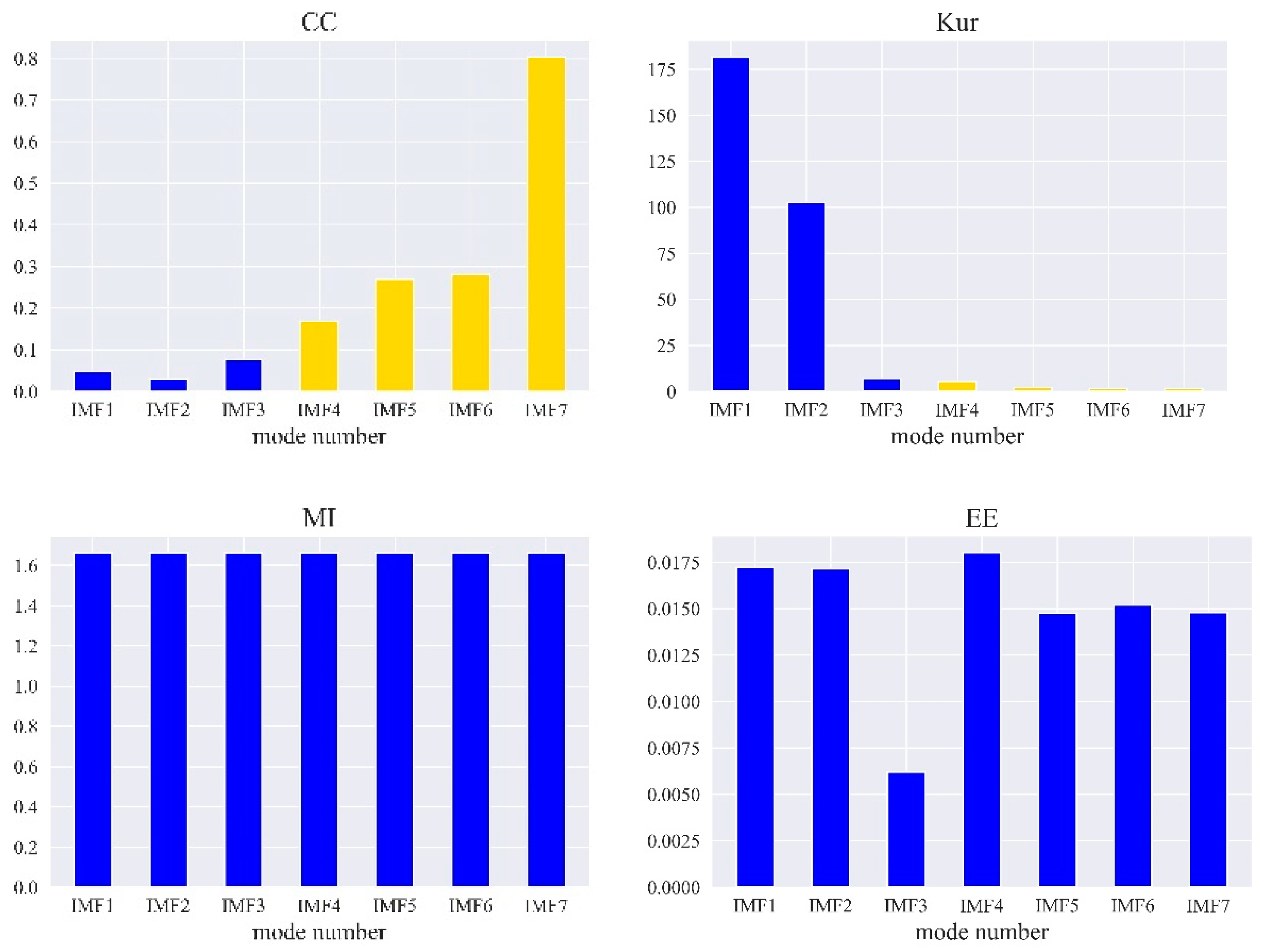
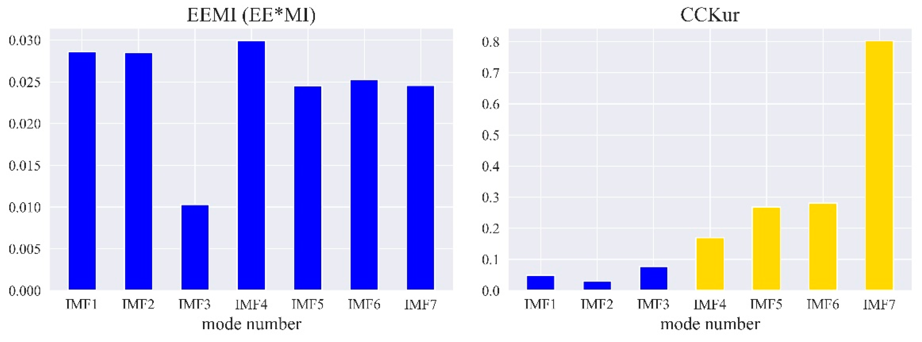
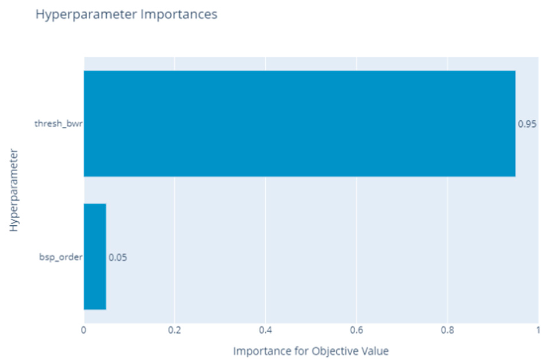
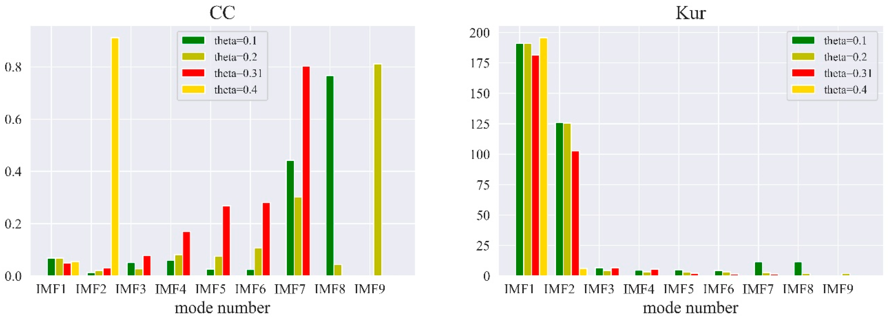
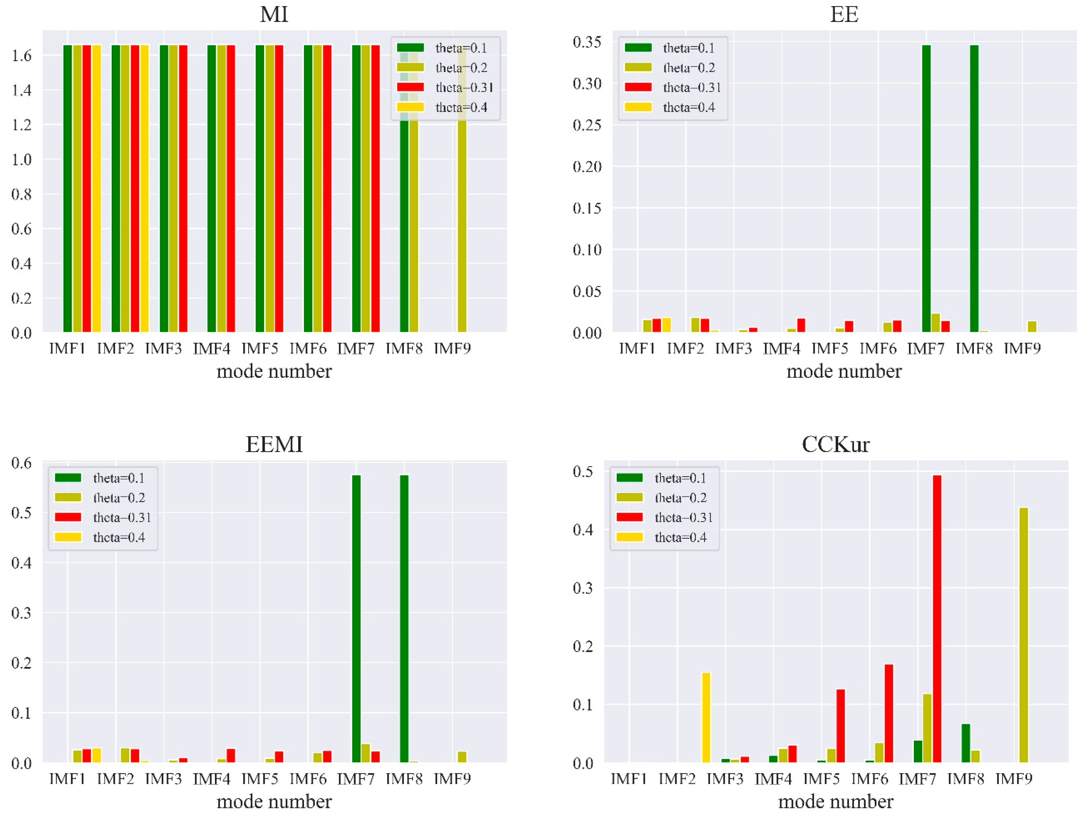
The hyperparameter $\xi$ was more important for decomposition results. The efficacy of the synthetic measurement index was verified against five optimization indices: CC, Kur, MI, EE, and EEMI on decomposed IMFs. The results demonstrated that the proposed CCKur index was sensitive to $\xi$, and the selection of CCKur as a synthetic measurement index and $\max \left\{CCKur\right\}$ as an objective function were reasonable and effective.

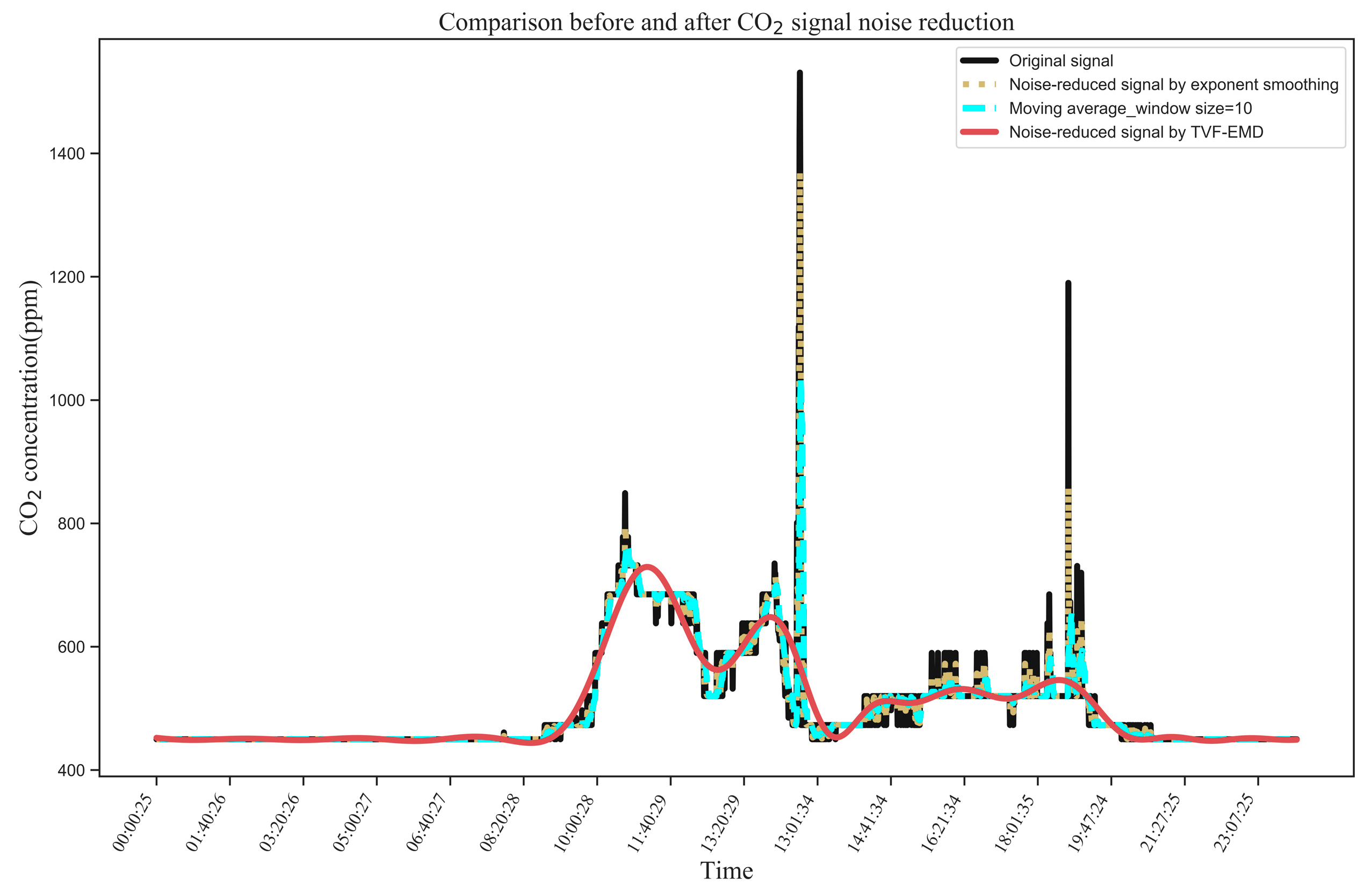
The noise reduction effect between different signal-denoising models, that is, TVF-EMD with default values, EMD, moving average method, and exponential smoothing method, was compared in terms of SNR, MSE, RSE, and NRMSE. The proposed noise cancellation model yielded the largest absolute value of SNR and the smallest MSE, RSE, and NRMSE, demonstrating the high noise reduction capability of the proposed model for CO₂ concentration signals.

References

1. Longo, A.; Bianchi, S.; Plastino, W. tvf-EMD based time series analysis of 7Be sampled at the CTBTO-IMS network. Phys. A Stat. Mech. Its Appl. 2019, 523, 908–914. [Google Scholar] [CrossRef] [Green Version]
2. Apte, M.G.; Fisk, W.J.; Daisey, J.M. Associations between indoor CO2 concentrations and sick building syndrome symptoms in US office buildings: An analysis of the 1994-1996 BASE study data. Indoor Air-Int. J. Indoor Air Qual. Clim. 2000, 10, 246–257. [Google Scholar] [CrossRef] [Green Version]
3. Muscatiello, N.; McCarthy, A.; Kielb, C.; Hsu, W.H.; Hwang, S.A.; Lin, S. Classroom conditions and CO2 concentrations and teacher health symptom reporting in 10 New York State Schools. Indoor Air 2015, 25, 157–167. [Google Scholar] [CrossRef] [PubMed]
4. Huang, N.E.; Shen, Z.; Long, S.R.; Wu, M.L.C.; Shih, H.H.; Zheng, Q.N.; Yen, N.C.; Tung, C.C.; Liu, H.H. The empirical mode decomposition and the Hilbert spectrum for nonlinear and non-stationary time series analysis. Proc. R. Soc. Lond. Ser. A Math. Phys. Eng. Sci. 1998, 454, 903–995. [Google Scholar] [CrossRef]
5. Wang, W.J.; McFadden, P.D. Application of wavelets to gearbox vibration signals for fault detection. J. Sound Vib. 1996, 192, 927–939. [Google Scholar] [CrossRef]
6. Huang, N.E.; Shen, Z.; Long, S.R. A new view of nonlinear water waves: The Hilbert Spectrum. Annu. Rev. Fluid Mech. 1999, 31, 417–457. [Google Scholar] [CrossRef] [Green Version]
7. Montesinos, M.E.; Muñoz-Cobo, J.L.; Pérez, C. Hilbert–Huang analysis of BWR neutron detector signals: Application to DR calculation and to corrupted signal analysis. Ann. Nucl. Energy 2003, 30, 715–727. [Google Scholar] [CrossRef]
8. Tian, P.; Cao, X.; Liang, J.; Zhang, L.; Yi, N.; Wang, L.; Cheng, X. Improved empirical mode decomposition based denoising method for lidar signals. Opt. Commun. 2014, 325, 54–59. [Google Scholar] [CrossRef]
9. Wu, S.; Liu, Z.; Liu, B. Enhancement of lidar backscatters signal-to-noise ratio using empirical mode decomposition method. Opt. Commun. 2006, 267, 137–144. [Google Scholar] [CrossRef]
10. Torrence, C.; Compo, G.P. A practical guide to wavelet analysis. Bull. Am. Meteorol. Soc. 1998, 79, 61–78. [Google Scholar] [CrossRef]
11. Huang, N.E.; Wu, Z.; Long, S.R. Hilbert-Huang transform. Scholarpedia 2008, 3, 2544. [Google Scholar] [CrossRef]
12. Li, H.; Li, Z.; Mo, W. A time varying filter approach for empirical mode decomposition. Signal Process. 2017, 138, 146–158. [Google Scholar] [CrossRef]
13. Wu, Z.; Huang, N.E. Ensemble empirical mode decomposition: A noise-assisted data analysis method. Adv. Adapt. Data Anal. 2009, 1, 1–41. [Google Scholar] [CrossRef]
14. Ur Rehman, N.; Mandic, D.P. Filter bank property of multivariate empirical mode decomposition. IEEE Trans. Signal Process. 2011, 59, 2421–2426. [Google Scholar] [CrossRef]
15. Rehman, N.; Mandic, D.P. Multivariate empirical mode decomposition. Proc. R. Soc. A Math. Phys. Eng. Sci. 2010, 466, 1291–1302. [Google Scholar] [CrossRef]
16. Stoica, P.; Gershman, A.B. Maximum-likelihood DOA estimation by data-supported grid search. IEEE Signal Process. Lett. 1999, 6, 273–275. [Google Scholar] [CrossRef]
17. Bellman, R.E.; Dreyfus, S.E. Applied Dynamic Programming; Princeton University Press: Princeton, NJ, USA, 2015; Volume 2050. [Google Scholar] [CrossRef]
18. Bergstra, J.; Bengio, Y. Random search for hyper-parameter optimization. J. Mach. Learn. Res. 2012, 13, 281–305. [Google Scholar]
19. Yang, X.-S. (Ed.) Chapter 6—Genetic Algorithms. In Nature-Inspired Optimization Algorithms, 2nd ed.; Academic Press: Cambridge, MA, USA, 2021; pp. 91–100. [Google Scholar] [CrossRef]
20. Frazier, P.I. A tutorial on Bayesian optimization. arXiv 2018, arXiv:1807.02811. [Google Scholar]
21. Shahriari, B.; Swersky, K.; Wang, Z.; Adams, R.P.; De Freitas, N. Taking the human out of the loop: A review of Bayesian optimization. Proc. IEEE 2015, 104, 148–175. [Google Scholar] [CrossRef] [Green Version]
22. Jones, D.R.; Schonlau, M.; Welch, W.J. Efficient global optimization of expensive black-box functions. J. Glob. Optim. 1998, 13, 455–492. [Google Scholar] [CrossRef]
23. Mirjalili, S. The ant lion optimizer. Adv. Eng. Softw. 2015, 83, 80–98. [Google Scholar] [CrossRef]
24. Marini, F.; Walczak, B. Particle swarm optimization (PSO). A tutorial. Chemom. Intell. Lab. Syst. 2015, 149, 153–165. [Google Scholar] [CrossRef]
25. Mirjalili, S.; Lewis, A. The whale optimization algorithm. Adv. Eng. Softw. 2016, 95, 51–67. [Google Scholar] [CrossRef]
26. Krishnanand, K.N.; Ghose, D. Glowworm swarm optimization for simultaneous capture of multiple local optima of multimodal functions. Swarm Intell. 2009, 3, 87–124. [Google Scholar] [CrossRef]
27. Mirjalili, S.; Mirjalili, S.M.; Lewis, A. Grey wolf optimizer. Adv. Eng. Softw. 2014, 69, 46–61. [Google Scholar] [CrossRef] [Green Version]
28. Zhou, C.; Xiong, Z.; Bai, H.; Xing, L.; Jia, Y.; Yuan, X. Parameter-Adaptive TVF-EMD Feature Extraction Method Based on Improved GOA. Sensors 2022, 22, 7195. [Google Scholar] [CrossRef]
29. Bergstra, J.; Bardenet, R.; Bengio, Y.; Kégl, B. Algorithms for hyper-parameter optimization. Adv. Neural Inf. Process. Syst. 2011, 24, 2546–2554. [Google Scholar]
30. Bergstra, J.; Yamins, D.; Cox, D. Making a science of model search: Hyperparameter optimization in hundreds of dimensions for vision architectures. In Proceedings of the 30th International Conference on Machine Learning, Atlanta, GA, USA, 17–19 June 2013; pp. 115–123. [Google Scholar]
31. Ozaki, Y.; Tanigaki, Y.; Watanabe, S.; Nomura, M.; Onishi, M. Multiobjective Tree-Structured Parzen Estimator. J. Artif. Intell. Res. 2022, 73, 1209–1250. [Google Scholar] [CrossRef]
32. Zhang, S.; Xu, F.; Hu, M.; Zhang, L.; Liu, H.; Li, M. A novel denoising algorithm based on TVF-EMD and its application in fault classification of rotating machinery. Measurement 2021, 179, 109337. [Google Scholar] [CrossRef]
33. Wang, J.; Liu, P.; Lu, S.; Zhou, M.; Chen, X. Decentralized plant-wide monitoring based on mutual information-Louvain decomposition and support vector data description diagnosis. ISA Trans. 2023, 133, 42–52. [Google Scholar] [CrossRef]
34. Gao, S.; Ren, Y.; Zhang, Y.; Li, T. Fault diagnosis of rolling bearings based on improved energy entropy and fault location of triangulation of amplitude attenuation outer raceway. Measurement 2021, 185, 109974. [Google Scholar] [CrossRef]
Figure 1. Flowchart of Bayesian optimization.
Algorithms 16 00296 g001
Figure 2. Flowchart for the noise-cancellation model.
Algorithms 16 00296 g002
Figure 3. Office CO2 concentrations throughout the day.
Algorithms 16 00296 g003
Figure 4. Decomposition results of the CO2 signal obtained by (a) EMD and (b) TVF-EMD.
Algorithms 16 00296 g004
Figure 5. Hurst exponent values in different modes.
Algorithms 16 00296 g005
Figure 6. Comparison of signal noise cancellation and the simulated CO2-concentration signal.
Algorithms 16 00296 g006
Figure 7. Relationship between IMF and the optimization index.
Algorithms 16 00296 g007aAlgorithms 16 00296 g007b
Figure 8. Hyperparameter importance in the decomposition result.
Algorithms 16 00296 g008
Figure 9. Relationship between IMF indices and the bandwidth threshold.
Algorithms 16 00296 g009aAlgorithms 16 00296 g009b