


Efficient DNN Model for Word Lip-Reading


Abstract
1. Introduction
2. Related Research
3. Basic Model
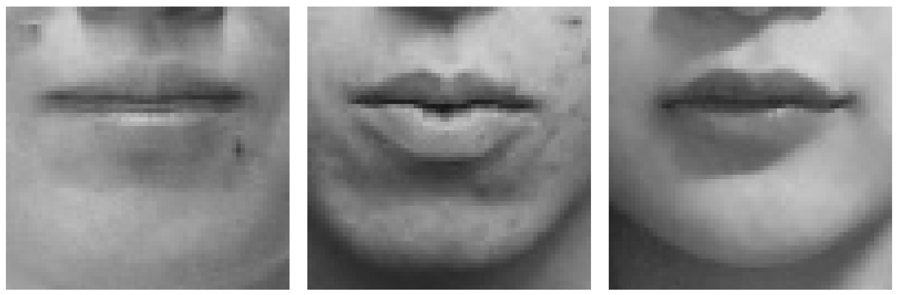
3.1. Preprocessing
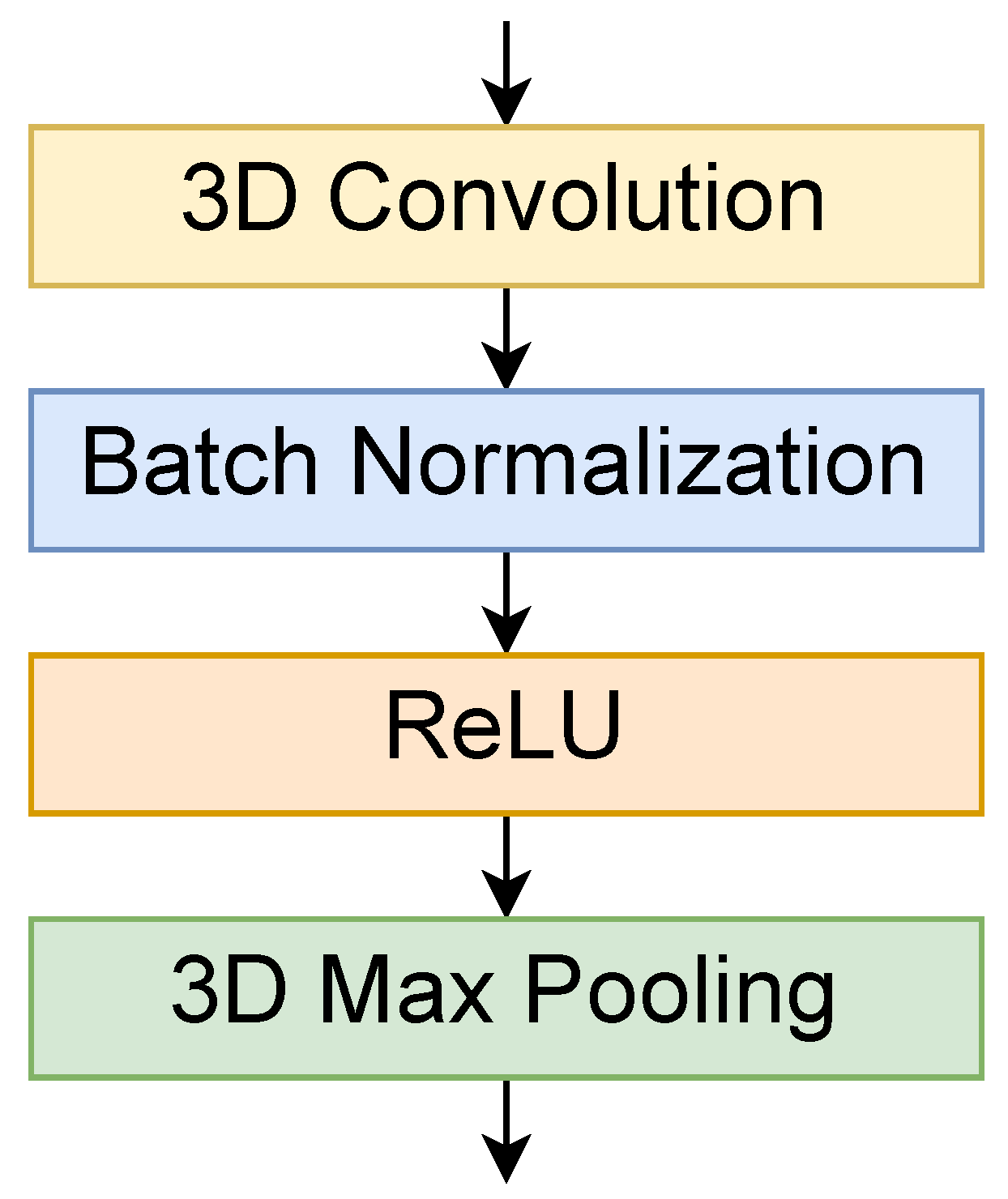
3.2. Three-Dimensional Convolution
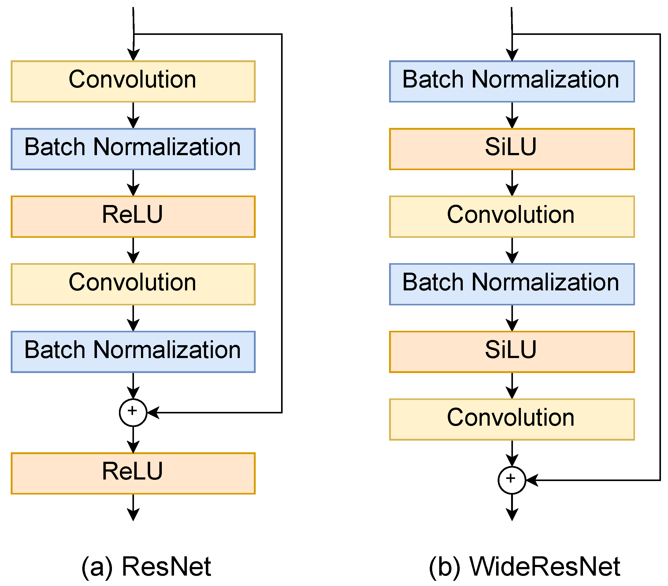
3.3. Resnet
3.4. WideResNet
3.5. EfficientNet
3.6. Transformer
3.7. ViT
3.8. ViViT
3.9. MS-TCN
3.10. Data Augmentation
3.11. Distance Learning
3.12. Fine-Tuning
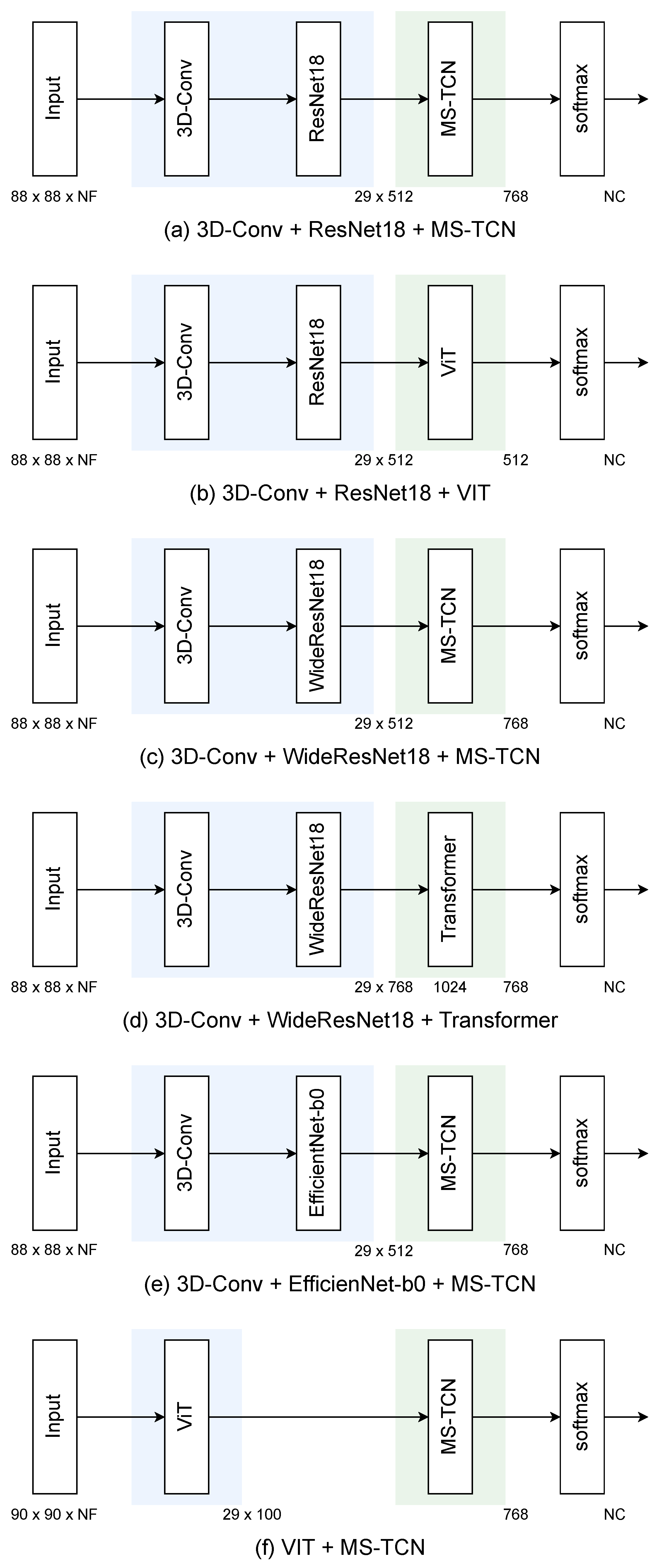
4. Target Models
4.1. 3D-Conv + ResNet18 + MS-TCN
4.2. 3D-Conv + ResNet18 + ViT
4.3. 3D-Conv + WiderResNet18 + MS-TCN
4.4. 3D-Conv + WiderResNet18 + Transformer
4.5. 3D-Conv + EfficientNet-b0 + MS-TCN
4.6. ViT + MS-TCN
5. Evaluation Experiment
5.1. LRW
5.2. OuluVS
5.3. CUAVE
5.4. SSSD
6. Conclusions
Author Contributions
Funding
Institutional Review Board Statement
Informed Consent Statement
Data Availability Statement
Conflicts of Interest
Abbreviations
| AE | Auto-Encoder |
| AU | Action Unit |
| BBC | British Broadcasting Corporation |
| BGRU | Bidirectional Gated Recurrent Unit |
| CNN | Convolutional Neural Network |
| DA | Data Augmentation |
| DC-TCN | Densely Connected Temporal Convolutional Network |
| FOMM | First-Order Motion Model |
| FT | Fine-Tuning |
| HOG | Histograms of Oriented Gradient |
| LN | Layer Normalization |
| LRW | Lip Reading in the Wild |
| LS | Label Smoothing |
| LSTM | Long Short-Term Memory |
| MF | Motion Feature |
| MLP | Multilayer Perceptron |
| MSA | Multi-head Self-Attention |
| MS-TCN | Multi-Scale Temporal Convolutional Network |
| NAS | Neural Architecture Search |
| RA | RandAugment |
| ResNet | Residual Network |
| RNN | Recurrent Neural Network |
| ROI | Region of Interest |
| RUSAVIC | Russian Audio-Visual Speech in Cars |
| SA | Squeeze-and-Attention |
| SiLU | Swish |
| SSSD | Speech Scene by Smart Device |
| SOTA | State of the Art |
| ViT | Vision Transformer |
| ViViT | Video Vision Transformer |
| WLAS | Watch, Listen, Attend, and Spell |
References
- Saitoh, T.; Konishi, R. Profile Lip Reading for Vowel and Word Recognition. In Proceedings of the 20th International Conference on Pattern Recognition (ICPR2010), Istanbul, Turkey, 23–26 August 2010. [Google Scholar] [CrossRef]
- Nakamura, Y.; Saitoh, T.; Itoh, K. 3D CNN-based mouth shape recognition for patient with intractable neurological diseases. In Proceedings of the 13th International Conference on Graphics and Image Processing (ICGIP 2021), Kunming, China, 18–20 August 2022; Volume 12083, pp. 775–782. [Google Scholar] [CrossRef]
- Kanamaru, T.; Arakane, T.; Saitoh, T. Isolated single sound lip-reading using a frame-based camera and event-based camera. Front. Artif. Intell. 2023, 5, 298. [Google Scholar] [CrossRef] [PubMed]
- Chung, J.S.; Zisserman, A. Lip Reading in the Wild. In Proceedings of the Asian Conference on Computer Vision (ACCV), Taipei, Taiwan, 20–24 November 2016. [Google Scholar]
- Shirakata, T.; Saitoh, T. Lip Reading using Facial Expression Features. Int. J. Comput. Vis. Signal Process. 2020, 10, 9–15. [Google Scholar]
- Martinez, B.; Ma, P.; Petridis, S.; Pantic, M. Lipreading using temporal convolutional networks. In Proceedings of the IEEE International Conference on Acoustics, Speech and Signal Processing (ICASSP), Barcelona, Spain, 4–8 May 2020; pp. 6319–6323. [Google Scholar] [CrossRef]
- Kodama, M.; Saitoh, T. Replacing speaker-independent recognition task with speaker-dependent task for lip-reading using First Order Motion Model. In Proceedings of the 13th International Conference on Graphics and Image Processing (ICGIP 2021), Kunming, China, 18–20 August 2022; Volume 12083, pp. 652–659. [Google Scholar] [CrossRef]
- Ma, P.; Martinez, B.; Petridis, S.; Pantic, M. Towards Practical Lipreading with Distilled and Efficient Models. In Proceedings of the IEEE International Conference on Acoustics, Speech and Signal Processing (ICASSP), Toronto, ON, Canada, 6–11 June 2021; pp. 7608–7612. [Google Scholar] [CrossRef]
- Fu, Y.; Lu, Y.; Ni, R. Chinese Lip-Reading Research Based on ShuffleNet and CBAM. Appl. Sci. 2023, 13, 1106. [Google Scholar] [CrossRef]
- Chung, J.S.; Senior, A.; Vinyals, O.; Zisserman, A. Lip Reading Sentences in the Wild. In Proceedings of the IEEE Conference on Computer Vision and Pattern Recognition (CVPR), Honolulu, HI, USA, 21–26 July 2017; pp. 6447–6456. [Google Scholar] [CrossRef]
- Arakane, T.; Saitoh, T.; Chiba, R.; Morise, M.; Oda, Y. Conformer-Based Lip-Reading for Japanese Sentence. In Proceedings of the 37th International Conference on Image and Vision Computing, Auckland, New Zealand, 24–25 November 2023; pp. 474–485. [Google Scholar] [CrossRef]
- Jeon, S.; Elsharkawy, A.; Kim, M.S. Lipreading Architecture Based on Multiple Convolutional Neural Networks for Sentence-Level Visual Speech Recognition. Sensors 2022, 22, 72. [Google Scholar] [CrossRef]
- Zhao, G.; Barnard, M.; Pietikainen, M. Lipreading with local spatiotemporal descriptors. IEEE Trans. Multimed. 2009, 11, 1254–1265. [Google Scholar] [CrossRef]
- Patterson, E.K.; Gurbuz, S.; Tufekci, Z.; Gowdy, J.N. Moving-talker, speaker-independent feature study, and baseline results using the CUAVE multimodal speech corpus. EURASIP J. Appl. Signal Process. 2002, 2002, 1189–1201. [Google Scholar] [CrossRef]
- Saitoh, T.; Kubokawa, M. SSSD: Speech Scene Database by Smart Device for Visual Speech Recognition. In Proceedings of the 24th International Conference on Pattern Recognition (ICPR2018), Beijing, China, 20–24 August 2018; pp. 3228–3232. [Google Scholar] [CrossRef]
- Yang, S.; Zhang, Y.; Feng, D.; Yang, M.; Wang, C.; Xiao, J.; Long, K.; Shan, S.; Chen, X. LRW-1000: A Naturally-Distributed Large-Scale Benchmark for Lip Reading in the Wild. In Proceedings of the 14th IEEE International Conference on Automatic Face & Gesture Recognition (FG2019), Lille, France, 14–18 May 2019. [Google Scholar] [CrossRef]
- Ivanko, D.; Ryumin, D.; Axyonov, A.; Kashevnik, A.; Karpov, A. Multi-Speaker Audio-Visual Corpus RUSAVIC: Russian Audio-Visual Speech in Cars. In Proceedings of the 13th Conference on Language Resources and Evaluation (LREC2022), Marseille, France, 21–23 June 2022; pp. 1555–1559. [Google Scholar]
- Ma, P.; Wang, Y.; Petridis, S.; Shen, J.; Pantic, M. Training Strategies for Improved Lip-reading. In Proceedings of the IEEE International Conference on Acoustics, Speech and Signal Processing (ICASSP), Singapore, 23–27 May 2022. [Google Scholar] [CrossRef]
- Feng, D.; Yang, S.; Shan, S.; Chen, X. Learn an Effective Lip Reading Model without Pains. arXiv 2020, arXiv:2011.07557. [Google Scholar] [CrossRef]
- Kim, M.; Yeo, J.H.; Ro, Y.M. Distinguishing Homophenes using Multi-head Visual-audio Memory for Lip Reading. In Proceedings of the 36th AAAI Conference on Artificial Intelligence (AAAI), Virtual, 22 February–1 March 2022. [Google Scholar]
- Koumparoulis, A.; Potamianos, G. Accurate and Resource-Efficient Lipreading with Efficientnetv2 and Transformers. In Proceedings of the 2022 IEEE International Conference on Acoustics, Speech and Signal Processing (ICASSP), Singapore, 23–27 May 2022. [Google Scholar] [CrossRef]
- Ivanko, D.; Ryumin, D.; Kashevnik, A.; Axyonov, A.; Karnov, A. Visual Speech Recognition in a Driver Assistance System. In Proceedings of the 30th European Signal Processing Conference (EUSIPCO), Belgrade, Serbia, 29 August–2 September 2022. [Google Scholar] [CrossRef]
- Szegedy, C.; Vanhoucke, V.; Ioffe, S.; Shlens, J.; Wojna, Z. Rethinking the Inception Architecture for Computer Vision. In Proceedings of the IEEE Conference on Computer Vision and Pattern Recognition (CVPR), Las Vegas, NV, USA, 27–30 June 2016; pp. 2818–2826. [Google Scholar] [CrossRef]
- Viola, P.; Jones, M. Rapid object detection using a boosted cascade of simple features. In Proceedings of the IEEE Computer Society Conference on Computer Vision and Pattern Recognition (CVPR), Kauai, HI, USA, 8–14 December 2001; Volume 1. [Google Scholar] [CrossRef]
- Dalal, N.; Triggs, B. Histograms of oriented gradients for human detection. In Proceedings of the IEEE Conference on Computer Vision and Pattern Recognition (CVPR), San Diego, CA, USA, 20–25 June 2005; Volume 1, pp. 886–893. [Google Scholar] [CrossRef]
- Deng, J.; Guo, J.; Ververas, E.; Kotsia, I.; Zafeiriou, S. RetinaFace: Single-Shot Multi-Level Face Localisation in the Wild. In Proceedings of the IEEE Conference on Computer Vision and Pattern Recognition (CVPR), Virtual, 14–19 June 2020; pp. 5203–5212. [Google Scholar]
- Kazemi, V.; Sullivan, J. One millisecond face alignment with an ensemble of regression trees. In Proceedings of the IEEE Conference on Computer Vision and Pattern Recognition (CVPR), Columbus, OH, USA, 24–27 June 2014; pp. 1867–1874. [Google Scholar] [CrossRef]
- He, K.; Zhang, X.; Ren, S.; Sun, J. Deep Residual Learning for Image Recognition. In Proceedings of the IEEE Conference on Computer Vision and Pattern Recognition (CVPR), Las Vegas, NV, USA, 26 June–1 July 2016; pp. 770–778. [Google Scholar] [CrossRef]
- Zagoruyko, S.; Komodakis, N. Wide Residual Networks. In Proceedings of the British Machine Vision Conference (BMVC), York, UK, 19–22 September 2016; pp. 87.1–87.12. [Google Scholar] [CrossRef]
- Tan, M.; Le, Q. EfficientNet: Rethinking Model Scaling for Convolutional Neural Networks. In Proceedings of the 36th International Conference on Machine Learning (ICMR), Long Beach, CA, USA, 9–15 June 2019. [Google Scholar]
- Zoph, B.; Le, Q.V. Neural architecture search with reinforcement learning. In Proceedings of the 5th International Conference on Learning Representations (ICLR), Toulon, France, 24–26 April 2017. [Google Scholar] [CrossRef]
- Vaswani, A.; Shazeer, N.; Parmar, N.; Uszkoreit, J.; Jones, L.; Gomez, A.N.; Kaiser, L.; Polosukhin, I. Attention Is All You Need. In Proceedings of the 31st Conference on Neural Information Processing Systems (NIPS2017), Long Beach, CA, USA, 4–9 December 2017. [Google Scholar]
- Dosovitskiy, A.; Beyer, L.; Kolesnikov, A.; Weissenborn, D.; Zhai, X.; Unterthiner, T.; Dehghani, M.; Minderer, M.; Heigold, G.; Gelly, S.; et al. An Image is Worth 16x16 Words: Transformers for Image Recognition at Scale. In Proceedings of the International Conference on Learning Representations (ICLR), Virtual, 3–7 May 2021. [Google Scholar]
- Arnab, A.; Dehghani, M.; Heigold, G.; Sun, C.; Lučić, M.; Schmid, C. ViViT: A Video Vision Transformer. In Proceedings of the IEEE/CVF International Conference on Computer Vision (ICCV), Virtual, 11–17 October 2021; pp. 6816–6826. [Google Scholar] [CrossRef]
- Bai, S.; Kolter, J.Z.; Koltun, V. An Empirical Evaluation of Generic Convolutional and Recurrent Networks for Sequence Modeling. arXiv 2018, arXiv:1803.01271. [Google Scholar] [CrossRef]
- Cubuk, E.D.; Zoph, B.; Shlens, J.; Le, Q. RandAugment: Practical Automated Data Augmentation with a Reduced Search Space. In Proceedings of the Advances in Neural Information Processing Systems, Virtual, 14–19 June 2020; Volume 33, pp. 18613–18624. [Google Scholar]
- Zhang, H.; Cisse, M.; Dauphin, Y.N.; Lopez-Paz, D. Mixup: Beyond empirical risk minimization. In Proceedings of the International Conference on Learning Representations (ICLR), Vancouver, BC, Canada, 30 April–3 May 2018. [Google Scholar] [CrossRef]
- Deng, J.; Guo, J.; Xue, N.; Zafeiriou, S. ArcFace: Additive Angular Margin Loss for Deep Face Recognition. In Proceedings of the IEEE/CVF Conference on Computer Vision and Pattern Recognition (CVPR), Long Beach, CA, USA, 16–20 June 2019; pp. 4685–4694. [Google Scholar] [CrossRef]
- Loshchilov, I.; Hutter, F. Decoupled weight decay regularization. In Proceedings of the International Conference on Learning Representations (ICLR), New Orleans, LA, USA, 6–9 May 2019. [Google Scholar] [CrossRef]
- Stafylakis, T.; Tzimiropoulos, G. Combining Residual Networks with LSTMs for Lipreading. In Proceedings of the Conference of the International Speech Communication Association (Interspeech 2017), Stockholm, Sweden, 20–24 August 2018; pp. 3652–3656. [Google Scholar]
- Petridis, S.; Stafylakis, T.; Ma, P.; Cai, F.; Tzimiropoulos, G.; Pantic, M. End-to-end Audiovisual Speech Recognition. In Proceedings of the IEEE International Conference on Acoustics, Speech, and Signal Processing (ICASSP), Calgary, AB, Canada, 15–20 April 2018; pp. 6548–6552. [Google Scholar]
- Tsourounis, D.; Kastaniotis, D.; Fotopoulos, S. Lip Reading by Alternating between Spatiotemporal and Spatial Convolutions. J. Imaging 2021, 7, 91. [Google Scholar] [CrossRef] [PubMed]
- Iwasaki, M.; Kubokawa, M.; Saitoh, T. Two Features Combination with Gated Recurrent Unit for Visual Speech Recognition. In Proceedings of the 14th IAPR Conference on Machine Vision Applications (MVA), Nagoya, Japan, 8–12 May 2017; pp. 300–303. [Google Scholar] [CrossRef]


| Name | Year | Language | # of Speakers | Content |
|---|---|---|---|---|
| LRW [4] | 2016 | English | 500 words | |
| OuluVS [13] | 2009 | English | 20 | 10 greeting phrases |
| CUAVE [14] | 2002 | English | 36 | 10 digits |
| SSSD [15] | 2018 | Japanese | 72 | 25 words |
| Model | Top-1 Acc. (%) | Params |
|---|---|---|
| Multi-Tower 3D-CNN [4] | 61.1 | — |
| WLAS [10] | 76.2 | — |
| 3D-Conv + ResNet34 + Bi-LSTM [40] | 83.0 | — |
| 3D-Conv + ResNet34 + Bi-GRU [41] | 83.39 | — |
| 3D-Conv + ResNet18 + MS-TCN [6] | 85.3 | — |
| 3D-Conv + ResNet18 + MS-TCN + MVM [20] | 88.5 | — |
| 3D-Conv + ResNet18 + MS-TCN + KD [8] | 88.5 | 36.4 |
| Alternating ALSOS + ResNet18 + MS-TCN [42] | 87.0 | 41.2 |
| Vosk + MediaPipe + LS + MixUp + SA | ||
| + 3D-Conv + ResNet-18 + BiLSTM + Cosine WR [22] | 88.7 | — |
| 3D-Conv + EfficientNetV2 + Transformer + TCN [21] | 89.5 | — |
| 3D-Conv + ResNet18 + {DC-TCN, MS-TCN, BGRU} (ensemble) | ||
| + KD + Word Boundary [18] | 94.1 | — |
| 3D-Conv + ResNet18 + MS-TCN (ours) | 87.4 | 36.0 |
| 3D-Conv + ResNet18 + MS-TCN + RA (ours) | 85.3 | 36.0 |
| 3D-Conv + ResNet18 + MS-TCN + ArcFace (ours) | 86.7 | 36.0 |
| 3D-Conv + ResNet18 + ViT (ours) | 83.8 | 30.1 |
| 3D-Conv + WideResNet18 + MS-TCN (ours) | 86.8 | 36.0 |
| 3D-Conv + WideResNet18 + Transformer (ours) | 79.2 | 11.2 |
| 3D-Conv + EfficientNet-b0 + MS-TCN (ours) | 80.6 | 32.3 |
| ViT + MS-TCN (ours) | 79.9 | 24.0 |
| ViViT (ours) | 72.4 | 3.9 |
| ViViT + RA (ours) | 75.6 | 3.9 |
| Order | Word | Top-1 Acc. (%) | Most Misrecognized Word |
|---|---|---|---|
| 486 | ABOUT | 64 | AMONG (10) |
| BECAUSE | 64 | ABUSE (10) | |
| 488 | ACTUALLY | 62 | ACTION (6) |
| COULD | 62 | EUROPEAN, SHOULD (4) | |
| MATTER | 62 | AMONG (6) | |
| NEEDS | 62 | YEARS (8) | |
| THINGS | 62 | YEARS (6) | |
| 493 | THEIR | 60 | THERE (20) |
| UNDER | 60 | DURING, LONDON (4) | |
| UNTIL | 60 | STILL (8) | |
| 496 | SPEND | 58 | SPENT (18) |
| THESE | 58 | THINGS (8) | |
| 498 | THING | 56 | BEING, NOTHING, THESE (4) |
| 499 | THINK | 50 | THING (16) |
| 500 | THERE | 44 | THEIR (12) |
| Model | Top-1 Acc. (%) |
|---|---|
| Multi-Tower 3D-CNN [4] | 91.4 |
| AE + GRU [43] | 81.2 |
| FOMM → AE + GRU [7] | 86.5 |
| {MF + AE + AU} + GRU [5] | 86.6 |
| 3D-Conv + ResNet18 + MS-TCN (ours) | 90.1 |
| 3D-Conv + ResNet18 + MS-TCN + RA (ours) | 93.1 |
| 3D-Conv + ResNet18 + MS-TCN + FT (ours) | 95.1 |
| 3D-Conv + ResNet18 + MS-TCN + RA + FT (ours) | 97.2 |
| Model | Top-1 Acc. (%) |
|---|---|
| AE + GRU [43] | 72.8 |
| FOMM → AE + GRU [7] | 79.8 |
| {MF + AE + AU} + GRU [5] | 83.4 |
| 3D-CNN (ours) | 84.4 |
| 3D-Conv + ResNet18 + MS-TCN (ours) | 87.6 |
| 3D-Conv + ResNet18 + MS-TCN + RA (ours) | 90.0 |
| 3D-Conv + ResNet18 + MS-TCN + FT (ours) | 93.7 |
| 3D-Conv + ResNet18 + MS-TCN + RA + FT (ours) | 94.1 |
| Model | Top-1 Acc. (%) |
|---|---|
| LipNet | 90.66 |
| 3D-Conv + ResNet18 + MS-TCN (ours) | 93.08 |
| 3D-Conv + ResNet18 + MS-TCN + RA (ours) | 93.68 |
| 3D-Conv + ResNet18 + MS-TCN + FT (ours) | 95.14 |
| 3D-Conv + ResNet18 + MS-TCN + RA + FT (ours) | 94.86 |
Disclaimer/Publisher’s Note: The statements, opinions and data contained in all publications are solely those of the individual author(s) and contributor(s) and not of MDPI and/or the editor(s). MDPI and/or the editor(s) disclaim responsibility for any injury to people or property resulting from any ideas, methods, instructions or products referred to in the content. |
© 2023 by the authors. Licensee MDPI, Basel, Switzerland. This article is an open access article distributed under the terms and conditions of the Creative Commons Attribution (CC BY) license (https://creativecommons.org/licenses/by/4.0/).
Share and Cite
Arakane, T.; Saitoh, T. Efficient DNN Model for Word Lip-Reading. Algorithms 2023, 16, 269. https://doi.org/10.3390/a16060269
Arakane T, Saitoh T. Efficient DNN Model for Word Lip-Reading. Algorithms. 2023; 16(6):269. https://doi.org/10.3390/a16060269
Chicago/Turabian StyleArakane, Taiki, and Takeshi Saitoh. 2023. "Efficient DNN Model for Word Lip-Reading" Algorithms 16, no. 6: 269. https://doi.org/10.3390/a16060269
APA StyleArakane, T., & Saitoh, T. (2023). Efficient DNN Model for Word Lip-Reading. Algorithms, 16(6), 269. https://doi.org/10.3390/a16060269