Recovering the Forcing Function in Systems with One Degree of Freedom Using ANN and Physics Information

Abstract

In engineering design, oftentimes a system’s dynamic response is known or can be measured, but the source generating these responses is not known. The mathematical problem where the focus is on inferring the source terms of the governing equations from the set of observations is known as an inverse source problem (ISP). ISPs are traditionally solved by optimization techniques with regularization, but in the past few years, there has been a lot of interest in approaching these problems from a deep-learning viewpoint. In this paper, we propose a deep learning approach—infused with physics information—to recover the forcing function (source term) of systems with one degree of freedom from the response data. We test our architecture first to recover smooth forcing functions, and later functions involving abruptly changing gradient and jump discontinuities in the case of a linear system. Finally, we recover the harmonic, the sum of two harmonics, and the gaussian function, in the case of a non-linear system. The results obtained are promising and demonstrate the efficacy of this approach in recovering the forcing functions from the data.

1. Introduction

Inverse problems are a special class of mathematical problems where the focus is on inferring causal relationships from the set of observations. These problems are often ill-posed and suffer from various numerical issues [1], however, are encountered extensively in different fields of science and engineering. In the past few decades, there has been a plethora of research on solving these problems [2,3,4].

A subclass of inverse problems, where, the interest is in estimating the right-hand side, or “source term”, of a governing equation, is known as inverse source problems (ISP). ISPs arise frequently in several domains of physics and engineering, a few noteworthy examples are the following: Optical Molecular Imaging (OMI), where the spatial distribution of bio-luminescent and fluorescent markers in the human tissues is reconstructed from light-intensity measurements [5,6]; Radiative Heat Transfer, where temperature distribution of a medium is reconstructed from radiation intensity measurements and medium properties [6]; Magnetoencephalography (MEG) and Electroencephalography (EEG), where surface electrical and magnetic current measurements on the head are used to determine the source of brain activity [7,8].

In this paper, we study one such ISP known as the dynamic load identification problem. Here, we attempt to recover the ‘forcing function’ or ‘excitation force’ of linear and non-linear oscillators from the dynamic response data. This problem can be solved both in the time and frequency domains; however, in this study, we adopt the time domain approach owing to its simplicity and straightforwardness.

In the past few decades, plenty of research has been published discussing various approaches to solving this problem, and it will be difficult to enumerate them all given the scope of this paper; nonetheless, a few notable mentions are as follows. Huang [9] used the conjugate gradient method to estimate the time-dependent forces in a non-linear oscillator. Ma et al. [10] developed a recursive estimator based on the Kalman filter to determine the impulsive load from the measurement data for the single and multi-degree-of-freedom systems. In another interesting work by Azam et al. [11], the authors proposed a dual Kalman filter for estimating the full states of a linear multi-degree of freedom system with unknown input from a limited number of noisy acceleration measurements and a known physical model. Ref. [12] formulated the force identification problem of the duffing oscillator as a Volterra-type integral equation of the first kind and used the regularization technique to stabilize the solution. Feldman [13] proposed a method for predicting forces only from response data without the need for any parametric or governing equation information using the Hilbert transform. Ref. [14] solved the non-linear force identification problem in the frequency domain using ordinary least squares with Tikhonov regularization and its variants. Liu et al. [15] solved the non-linear vibration problem by transforming the non-linear ordinary differential equations into parabolic ordinary differential equations due to their robustness against large noise. Recently, Rice et al. [16] proposed a calibration-based integral formulation for estimating the forcing function in the spring mass damper system from response data. For a detailed review of past and present literature on dynamic load identification techniques, interested readers are advised to refer to [17].

In recent years, there has been a significant interest in applying machine learning and deep learning techniques for load identification. Pravin and Rao [18] proposed a technique for recovering the input forces from acceleration time history using dynamic principal component analysis. Zhou et al. [19] used a deep Recurrent Neural Networks (RNNs) technique with two variants of Long Short Term Memory (LSTM) to recover the impact loads on non-linear structures from response data. They tested their architecture on a damped duffing oscillator subjected to an impact load expressed by normal distribution function and on a composite plate. Another work [20] proposed RNN with different architecture, but this work was mainly focused on recovering the forces on beam structure excited by harmonic, impact, and random forces. In another work by Luca Rosafalco et al. [21], the authors implemented a deep learning based autoencoder for load identification, for structural health monitoring, from multivariate structural vibration data. They employed residual learning and inception modules in their autoencoder network. Ref. [22] proposed an ANN based on Bayesian Probability Framework to estimate the forces from the displacement responses.

In spite of the massive success of deep learning techniques in tackling a variety of problems owing to their ability to explore vast design space and to manage ill-posed problems, deep learning predictions are oftentimes physically inconsistent and generalize poorly [23]. However, this behavior can be alleviated to some extent by embedding various biases; one way of achieving this is by infusing the governing equation in the loss function of a neural network as proposed by [24], known as a “physics-informed neural network (PINNs). Recently, PINNs have been used to solve inverse source problems; one such account is the paper by He et al. [25]. In this work, the author utilized PINNs to predict the spatially and temporally varying heat source from the simulated temperature data with good accuracy. In this work, we use the PINNs approach for estimating the forcing function of one degree of freedom system.

Recently, two studies [26,27] have been published where the authors utilized machine learning and physics information to solve the vibration problem. The former used the Hilbert transform and a variant of the least-squares method to estimate the non-linear restoring force in a bi-stable structure, and the latter used PINNs to solve forced vibration and plate vibration problems.

Haghighat et al. [27] also used PINNs to solve forced spring mass damper systems similar to ours, but their work was mostly about predicting the displacements for a future time step and natural frequency, whereas our approach is more focused on estimating the excitation forces. We propose PINNs to estimate harmonic or non-harmonic and periodic or aperiodic forcing functions for systems with one degree of freedom subjected to various initial conditions.

Although in this work our attention is on oscillators as a mechanical system, to our understanding, this work also has the potential to be applied to any systems governed by linear or non-linear ordinary differential equations in different domains.

The remainder of the paper is organized as follows: In Section 2, we talk about the mathematical model of duffing’s equation followed by Section 3 where we discuss the structure of our neural network and share details about the training process. Later, in the following Section 4, we share our findings and finally conclude this paper with Section 5 and Section 6 with discussions and conclusions, respectively.

2. Mathematical Model

Duffing’s equation is a nonlinear ordinary differential equation used to model the approximate behavior of various physical systems, such as nano-mechanical resonators [28], ultrasonic cutting systems [29], piezo-ceramics under influence of a magnetic field, and, the flight motor of an insect [30], to name a few. One formulation of Duffing’s equation is given by

$$\begin{array}{c}\hfill \ddot{x}+\delta \dot{x}+\alpha x+\beta x^3=f\left(t\right).\end{array}$$

(1)

Here, $x\left(t\right)$ is the solution to a differential equation. Initial conditions are given by $x\left(0\right)=x_0$ and $\dot{x}\left(0\right)={\dot{x}}_0$, $\delta$ is the amount of damping, $\alpha$ is linear stiffness, $\beta$ is the amount of non-linearity, and $f\left(t\right)$ is the forcing function. By rearranging and fixing different values of coefficients, i.e., $\alpha ,\delta ,\beta$ in Equation (1), the governing equation of various linear and non-linear oscillators can be derived. 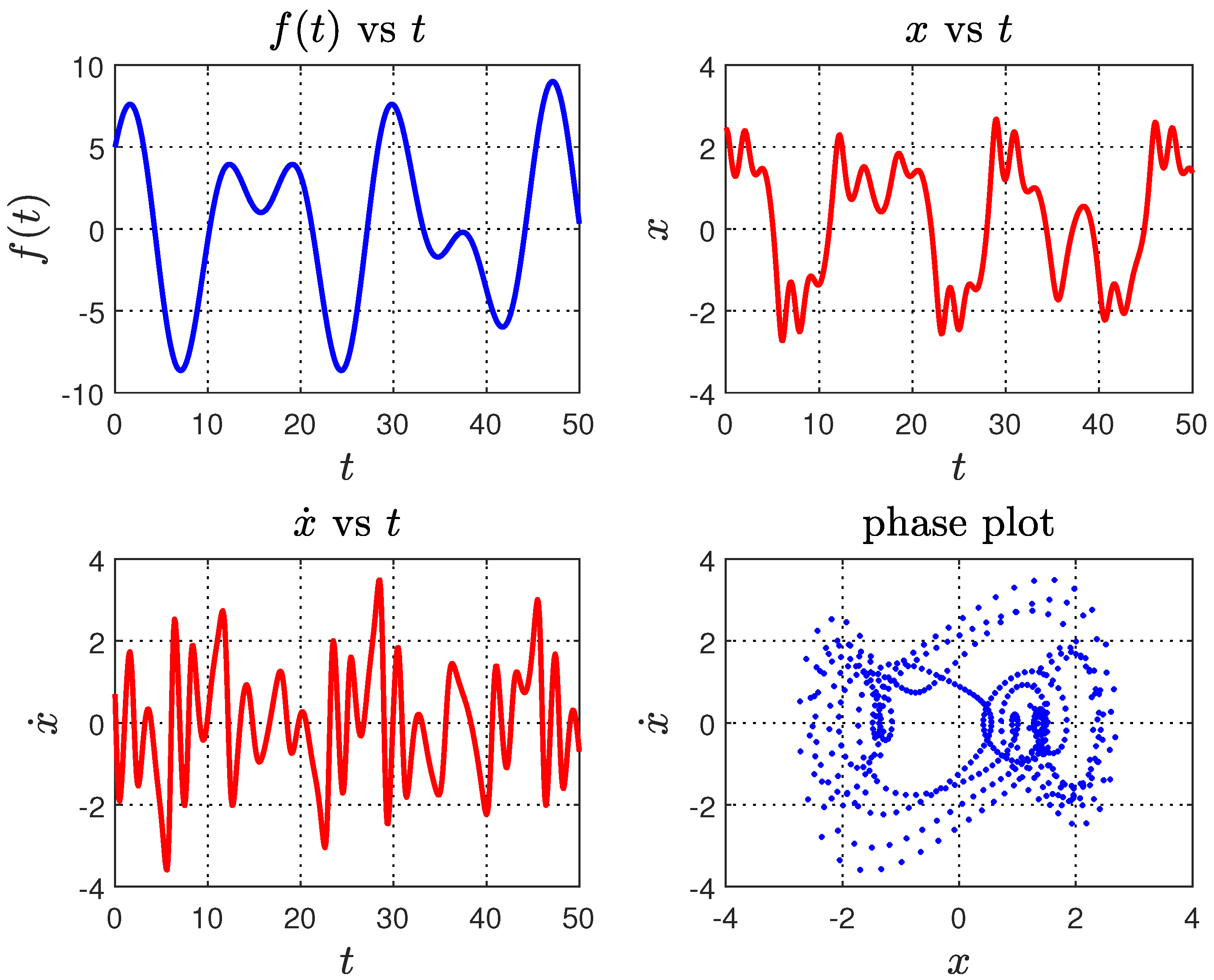For a detailed mathematical treatment and understanding of Duffing’s equation, interested readers are advised to refer to [31].

In this work, we are going to recover $f\left(t\right)$ from the simulated measurement of $x\left(t\right)$, its derivative $\dot{x}\left(t\right)$, and initial conditions using artificial neural network (ANN) and governing equation information. This is different than solving in a forward manner, where we typically solve the differential equation analytically or numerically, to get the solution $x\left(t\right)$ given $f\left(t\right)$ and initial conditions.

3. Methodology

In this section, we discuss the structure of the neural network (NN) that was used, followed by details on the loss function, and later, sum up the section by shedding some light on the training algorithm and process that was employed.

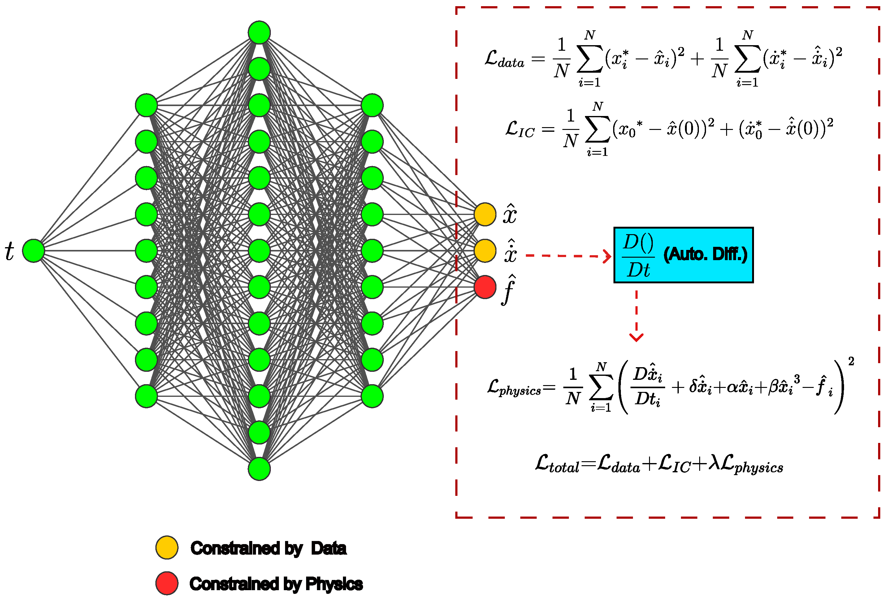
3.1. Structure of NN

The structure of NN is shown in Figure 1 and mathematically is represented by

$$\begin{array}{c}\hfill \widehat{f},\widehat{x},\widehat{\dot{x}}={\mathsf{\Phi }}^L(t;\mathbf{W},\mathbf{b})\end{array}$$

(2)

where the function ${\mathsf{\Phi }}^L:{\mathbb{R}}^{+}\mapsto {\mathbb{R}}^3$ represents the neural network with L number of layers; $t\in {\mathbb{R}}^{+}$ is the input and $\widehat{x}\in \mathbb{R}$, $\widehat{\dot{x}}\in \mathbb{R}$, $\widehat{f}\in \mathbb{R}$ are the outputs; $\mathbf{W}\in {\mathbb{R}}^{n\times n}$ and $\mathbf{b}\in {\mathbb{R}}^n$ are the neural network parameters. The architecture was defined in this way since it makes the differentiation of NN output with respect to input more manageable. Differentiation was performed using Automatic Differentiation (AD) with the help of the TensorFlow [32] library functions.

The NN is feed-forward in a sense, such that the first layer is an input to the second, and the second to the next, and so on until the last layer. This can be represented by the composite equation below,

$$\begin{array}{c}\hfill {\mathbf{x}}^j={\sigma }^j({\mathbf{W}}^j·{\mathbf{x}}^{j-1}+{\mathbf{b}}^j),j\in \{0,\dots ,L\}\end{array}$$

(3)

where j is the layer number, ${\sigma }^j:{\mathbb{R}}^n\mapsto {\mathbb{R}}^n$ is the activation function which adds non-linearity to the NN, and ${\mathbf{W}}^j$ and ${\mathbf{b}}^j$ are weights and biases of the specific layer.

For example, a 4-layer neural network, i.e., $L=4$, can be represented by

$$\begin{array}{cc}\hfill {\mathbf{x}}^1& ={\sigma }^1\left({\mathbf{W}}^1·{\mathbf{x}}^0+{\mathbf{b}}^1\right)\hfill \\ \hfill {\mathbf{x}}^2& ={\sigma }^2\left({\mathbf{W}}^2·{\mathbf{x}}^1+{\mathbf{b}}^2\right)\hfill \\ \hfill {\mathbf{x}}^3& ={\sigma }^3\left({\mathbf{W}}^3·{\mathbf{x}}^2+{\mathbf{b}}^3\right)\hfill \\ \hfill {\mathbf{x}}^4& ={\mathbf{W}}^4·{\mathbf{x}}^3+{\mathbf{b}}^4\hfill \end{array}$$

(4)

where ${\mathbf{x}}^0=t$ and ${\mathbf{x}}^4=[\widehat{f},\widehat{x},\widehat{\dot{x}}]$. The output of NN, $\widehat{f}$ is constrained by the physical model and $\widehat{x}$, $\widehat{\dot{x}}$ are constrained by the displacement and velocity data, respectively. This is discussed in more detail in the Section 3.2.

The proposed NN architecture was developed using the Keras [33] library with a TensorFlow backend. It consists of $L=10$ layers with [1,15,30,60,120, 240,120,60,30,15,3] units each. The batch normalization layer is present alternately after every dense layer and, each dense layer is passed through the eLU activation function, which adds the non-linearity to the network.

The optimal hyper-parameters were determined by performing systematic hyper-parameter tuning, which involved exploring different combinations of neural network architectures, initialization methods, activation functions, learning rates, and number of epochs. Initially, a shallow network with a smaller number of trainable parameters and ReLU activation function was used, but this did not yield satisfactory results. Subsequently, other activation functions were experimented with, and it was found that the eLU activation function produced better results. Finally, a deeper architecture with eLU activation function was employed. Similar experiments were conducted to identify other optimal hyper-parameter choices. Additional optimal hyper-parameters choices used in study are discussed in the Section 3.3.

3.2. Loss Function

The workhorse of our approach is the way the neural network loss function is defined. The total loss ${\mathcal{L}}_{total}$ is composed of the data term ${\mathcal{L}}_{data}$, ${\mathcal{L}}_{IC}$ and the physics loss term ${\mathcal{L}}_{physics}$:

$$\begin{array}{c}\hfill {\mathcal{L}}_{total}={\mathcal{L}}_{data}+{\mathcal{L}}_{IC}+\lambda {\mathcal{L}}_{physics}\end{array}$$

(5)

such that

$$\begin{array}{c}\hfill {\mathcal{L}}_{data}=\frac{1}{N}\sum _{i=1}^N{(x_i^{*}-{\widehat{x}}_i)}^2+\frac{1}{N}\sum _{i=1}^N{({\dot{x}}_i^{*}-{\widehat{\dot{x}}}_i)}^2\end{array}$$

(6)

and

$$\begin{array}{c}\hfill {\mathcal{L}}_{IC}={(x_0-\widehat{x}\left(0\right))}^2+{({\dot{x}}_0-\widehat{\dot{x}}(0))}^2.\end{array}$$

(7)

Here, $x_i^{*}$ and ${\dot{x}}_i^{*}$ are the displacement and velocity from the data, ${\widehat{x}}_i$ and ${\widehat{\dot{x}}}_i$ are displacement and velocity predictions from the neural network, $\lambda$ represents the regularization term, $x_0$ and ${\dot{x}}_0$ are the initial conditions.The task of ${\mathcal{L}}_{data}$ and ${\mathcal{L}}_{IC}$ is to constrain the neural network predictions using the data.

The physics loss ${\mathcal{L}}_{physics}$ term is where the physics information is infused into the neural networks and is given by,

$$\begin{array}{c}\hfill {\mathcal{L}}_{physics}=\frac{1}{N}\sum _{i=1}^N{\left(\frac{D{\widehat{\dot{x}}}_i}{D{t}_i}+\delta {\widehat{\dot{x}}}_i+\alpha {\widehat{x}}_i+\beta {{\widehat{x}}_i}^3-{\widehat{f}}_i\right)}^2.\end{array}$$

(8)

This equation is obtained by rearranging Equation (1) and replacing velocities and displacements with their equivalent neural network predictions. For calculating the acceleration from velocity prediction, we make use of automatic differentiation, which is represented by ${\displaystyle \frac{D}{D{t}_i}}$ in the above equation. The job of ${\mathcal{L}}_{physics}$ is to force the ${\widehat{f}}_i$ to take values that obey the governing equation.

3.3. Training

The objective of the proposed NN architecture is to recover the forcing function, $f\left(t\right)$, from the displacement and velocity data. The training algorithm is shown below (refer to Algorithm 1). Inputs to the algorithm are t, $x^{*}$,${\dot{x}}^{*}$, i.e., time, displacement, and velocity data. The NN takes in t and outputs $\widehat{f},\widehat{x},\widehat{\dot{x}}$, i.e., forcing function, displacement, and velocity predictions, respectively. The weights of the neural network are initialized using He-Normal initialization.

The network was trained on 500 data points in batches of 250 points on NVIDIA GTX 2060 GPU for 60,000 epochs. The training time for all the training instances was around 3 to 3.5 h approximately. The learning rate $\eta$ was chosen as 0.001 and the regularization term $\lambda$ was chosen as either 0.1 or 0.01 depending on which provided a better result.

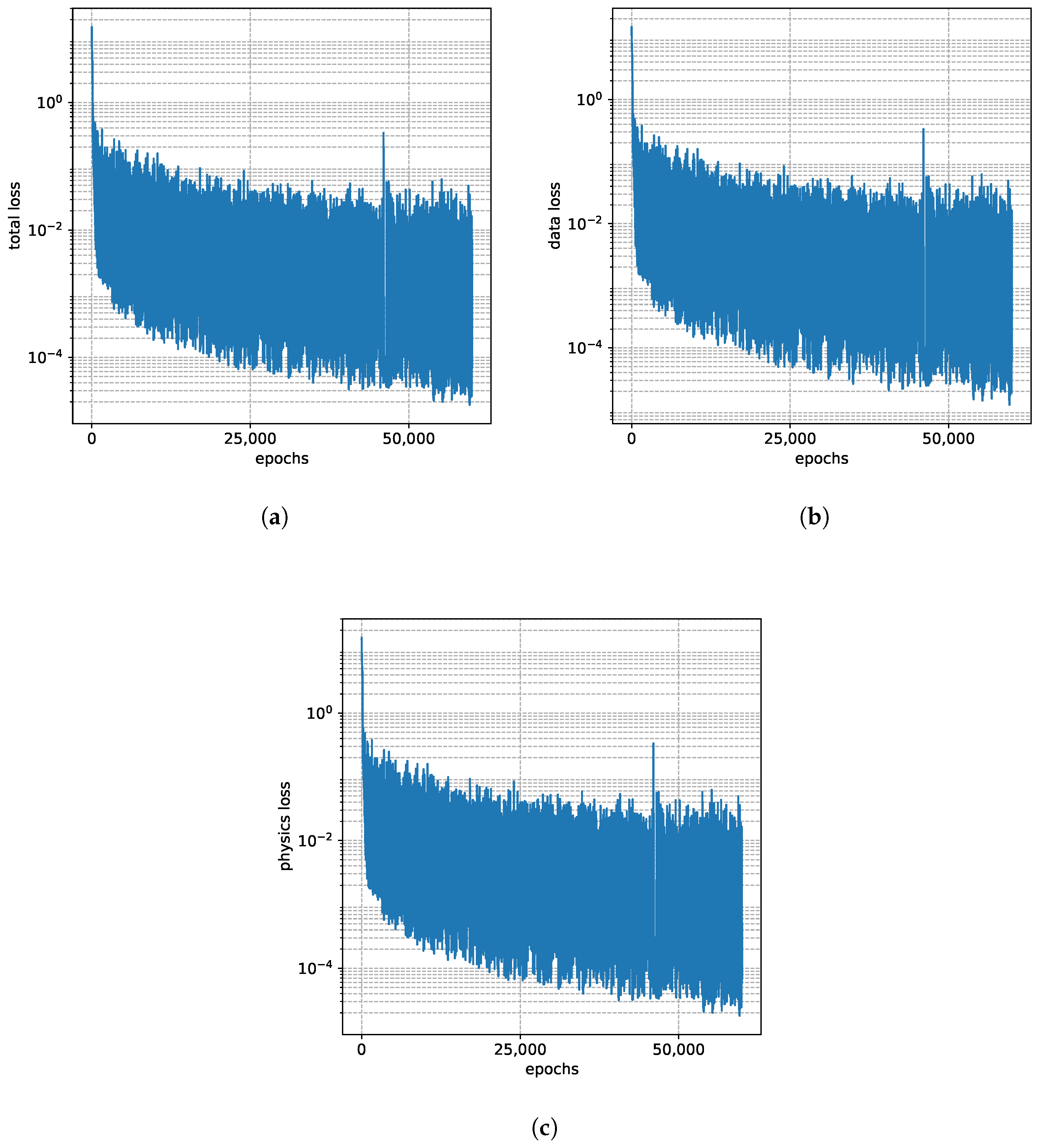
At each epoch, the ${\mathcal{L}}_{total}$ is calculated from the data and neural network predictions. Later, Adam optimizer [34] takes in ${\mathcal{L}}_{total}$ and calculates its gradients with respect to NN parameters and propagates them to the network using the back-propagation algorithm. This algorithm uses these gradients to adjust the weights and biases of the network at every epoch. A snapshot of ${\mathcal{L}}_{total}$, ${\mathcal{L}}_{data}$ and ${\mathcal{L}}_{physics}$ progression with respect to epochs for one training instance is shown in the Figure 2. Ideally, for the neural network to learn successfully ${\mathcal{L}}_{total}\to 0$, which can be observed in the Figure 2 below.

Algorithm 1 Training Algorithm

Require: t, $x^{*}$, ${\dot{x}}^{*}$ Ensure: ${\mathcal{L}}_{total}\to 0$  $n\leftarrow$ no. of epochs  $\eta \leftarrow$ learning rate  $N\leftarrow$ batch size  $\lambda \leftarrow$ regularization  while $n>0$ do       $\widehat{f},\widehat{x},\widehat{\dot{x}}\leftarrow {\mathsf{\Phi }}^L(t;\mathbf{W},\mathbf{b})$       ${\mathcal{L}}_{data},{\mathcal{L}}_{IC},{\mathcal{L}}_{physics}$       ▹ This is calculated using (6)–(8)       ${\mathcal{L}}_{total}\leftarrow {\mathcal{L}}_{data}+{\mathcal{L}}_{IC}+\lambda {\mathcal{L}}_{physics}$       ${\mathbf{W}}^{*},{\mathbf{b}}^{*}\leftarrow$ Adam($\eta ,{\mathcal{L}}_{total}$)       $\mathbf{W},\mathbf{b}\leftarrow {\mathbf{W}}^{*},{\mathbf{b}}^{*}$       $n\leftarrow n-1$  end while

4. Results

In this section, we share our findings that were obtained by performing various numerical experiments on our proposed architecture. We start by discussing the results of spring mass damper systems excited by different types of forces and initial conditions and later sum up the section on the results of our experiments with the non-linear oscillator.

The data for training the neural network were generated by simulating Equation (1) using the ode45 routine of MATLAB [35] for different coefficients $\alpha ,\beta ,\delta$ and initial conditions $x_0,{\dot{x}}_0$, for all the simulations, $t\in [0,50 \mathrm{s}]$. A snapshot of data instance that was generated by simulating ODE is shown in Figure 3.

4.1. Linear Case

We convert Equation (1) to a linear ODE by setting $\beta =0$. Later, by fixing $\alpha =k/m$, $\delta =c/m$ and $f\left(t\right)=f\left(t\right)/m$ the equation reduces to an equivalent spring mass damper system with mass m, stiffness c and spring constant k. For the remainder of this section, we consider $m=1$, $c=0.2$ and $k=0.9$ or equivalently $\alpha =0.9$, $\delta =0.2$. Finally, data are generated by solving the linear ODE subjected to sinusoidal, piece-wise, and step-forcing functions.

The neural network was trained on generated data instances and was tested to determine if it can recover the forcing functions from these data. The following sections provide more details of the results that were obtained after training.

4.1.1. Sinusoidal Function

To test whether the neural network can recover a smooth periodic function, we train it on the data generated by subjecting the spring mass damper system to a harmonic excitation given by

$$\begin{array}{c}\hfill f\left(t\right)=\gamma cos\omega t\end{array}$$

(9)

with $x_0=4.9,{\dot{x}}_0=-2.2,\omega =0.4$, and $\gamma =3$. The result obtained is promising and is shown in Figure 4a. It can be observed that the NN prediction and actual function are in excellent agreement.

4.1.2. Piece-Wise Function

Here, we subject the spring mass damper system to piece-wise forcing functions represented by equations,

$$\begin{array}{c}\hfill f\left(t\right)=\left\{\begin{array}{cc}0\hfill & 0\le t<5\hfill \\ t-5\hfill & 5\le t<10\hfill \\ {\displaystyle \frac{5}{20}}(30-t)\hfill & 10\le t<30\hfill \\ 0\hfill & 30\le t\le 50\hfill \end{array}\right.\end{array}$$

(10)

and,

$$\begin{array}{c}\hfill f\left(t\right)=\left\{\begin{array}{cc}{t}^2\hfill & 0\le t<10\hfill \\ -2t+120\hfill & 10\le t<30\hfill \\ {\displaystyle \frac{1}{200}}{t}^3-{\displaystyle \frac{1}{2}}{t}^2+{\displaystyle \frac{25}{2}}t\hfill & 30\le t\le 50\hfill \end{array}\right.\end{array}$$

(11)

the former represents a triangular function, consisting of linearly increasing and decreasing functions at consecutive intervals and the latter is a combination of parabolic, linear, and cubic functions. The functions are characterized by abrupt variations in gradient magnitudes.

Figure 5b,c demonstrate our findings where the network was trained on data instances generated by simulating the spring mass damper system for $x_0=4.4,{\dot{x}}_0=-4.4$, and $x_0=2.2$, ${\dot{x}}_0=-3.8$ initial conditions subjected to forces represented by Equations (10) and (11), respectively.

As observed, the actual forcing function and neural network predictions match very well; however, the network experiences some challenges in predicting the values at the cusp of both functions. For the triangular function, it under-predicts, and for the combination of linear, parabolic, and cubic it over-predicts. In addition, for the interval with a zero value of the function, marking the start of the triangular function, some oscillations are observed in the network predictions.

4.1.3. Step Function

After testing our architecture to recover the piece-wise forcing function in the previous section. In the present section, we attempt to solve a problem that is much more challenging. We try to determine if our architecture can recover functions involving discontinuities. To answer this question we train the neural network on the data generated by simulating the spring mass damper system with $x_0=-3.4,{\dot{x}}_0=-2.4$ and step function below,

$$\begin{array}{c}\hfill f\left(t\right)=\left\{\begin{array}{cc}0\hfill & 0\le t<5\hfill \\ 10\hfill & 5\le t<10\hfill \\ -10\hfill & 10\le t<30\hfill \\ 0\hfill & 30\le t\le 50\hfill \end{array}\right.\end{array}$$

(12)

A step function is marked by constant values on specific intervals followed by sudden jumps in values at the point of transition.

Figure 5d shows our findings. It can be observed NN was able to recover the majority of the function from the data. The constant values of the step function are complemented with oscillatory predictions. These oscillations resemble the Gibbs phenomenon, which is observed when approximating functions with jump discontinuities using the Fourier series.

4.2. Non-Linear Case

After our success with linear ODE in the previous sections, we now evaluate the effectiveness of our proposed architecture on non-linear ODE. We subject Equation (1) to different smooth forcing functions such as sinusoidal, the sum of two sinusoidal, and impulse functions. We share details and findings of our numerical experiments in the following section.

4.2.1. Sinusoidal Function

We solve the governing Equation (1) by subjecting it to the sinusoidal forcing function given by,

$$\begin{array}{c}\hfill f\left(t\right)=\gamma cos\omega t\end{array}$$

(13)

fixing $\alpha =1,\delta =1,\beta =0.5,\gamma =3,\omega =0.4$ and initial conditions $x_0=0.6$ ${\dot{x}}_0=1.4$ to generate the response data.

Figure 4a demonstrates the performance of our network after training it on the generated data. It can be observed that the neural network was successful in accurately recovering the sinusoidal function from response data without much difficulty; nonetheless, there exists some instability at the starting point.

We now increase the difficulty by setting $\alpha =0.6,\delta =0.3,\beta =1.2,\gamma =3,\omega =0.7$ and initial conditions $x_0=0.2,{\dot{x}}_0=0.7$. An interesting thing to note here is that the non-linearity $\beta =1.2$ and frequency $\omega =0.7$ are now increased versus the previous case.

The finding for this case is shown in Figure 4b. Although seen network predictions are in good agreement with the actual function, for the most part, the neural network over-predicts at the peaks and valleys with the presence of some instabilities at the start of the function.

4.2.2. Sum of Two Sinusoidal Functions

In this section, we attempt to recover the forcing function represented by the sum of two sinusoidal functions represented by the following equation,

$$\begin{array}{c}\hfill f\left(t\right)={\gamma }_{1}cos{\omega }_{1}t+{\gamma }_{2}cos{\omega }_{2}t\end{array}$$

(14)

The neural network was trained on the data that were generated by fixing the values of $\alpha =0.4,\beta =0.9,\delta =0.5$ and solving the duffing equation subjected to Equation (14) with ${\gamma }_1=5,{\gamma }_2=4,{\omega }_1=0.4,{\omega }_2=0.7$ and $x_0=2.4 {\dot{x}}_0=0.7$ initial conditions. This is somewhat more difficult compared to the previous case involving just one sinusoidal function. The results are shown in Figure 4c, it can be seen that the NN was able to predict the forcing function from response data with acceptable accuracy. Although NN does under-predict and over-predict at certain peaks and valleys of the function, nevertheless, overall the actual function and predictions are almost perfectly aligned.

4.2.3. Impulse Function Idealized by Normal Distribution

Finally, in the present section, we evaluate the efficacy of our network in predicting an impulsive function expressed by a normal distribution given by,

$$\begin{array}{c}\hfill f\left(t\right)=\frac{e^{-{(t-\mu )}^2/\left(2{\sigma }^2\right)}}{\sigma \sqrt{2\pi }}.\end{array}$$

(15)

We set $\mu =25,$ and $\sigma =2$ in Equation (15) and use this to produce the data by simulating Equation (1) with $\alpha =0.4,\beta =1.4,\delta =0.6$ and $x_0=1,{\dot{x}}_0=-2.2$. This case was used to test if the network can predict an impact excitation force of non-linear oscillators. For the purpose of smoothness, the impact force was expressed by a normal distribution equation. As seen in Figure 4d, the network predictions start with numerical oscillations that later damp out, and, for the most part, the predictions are in good alignment with the actual forcing function that was used for generating the data.

5. Discussion

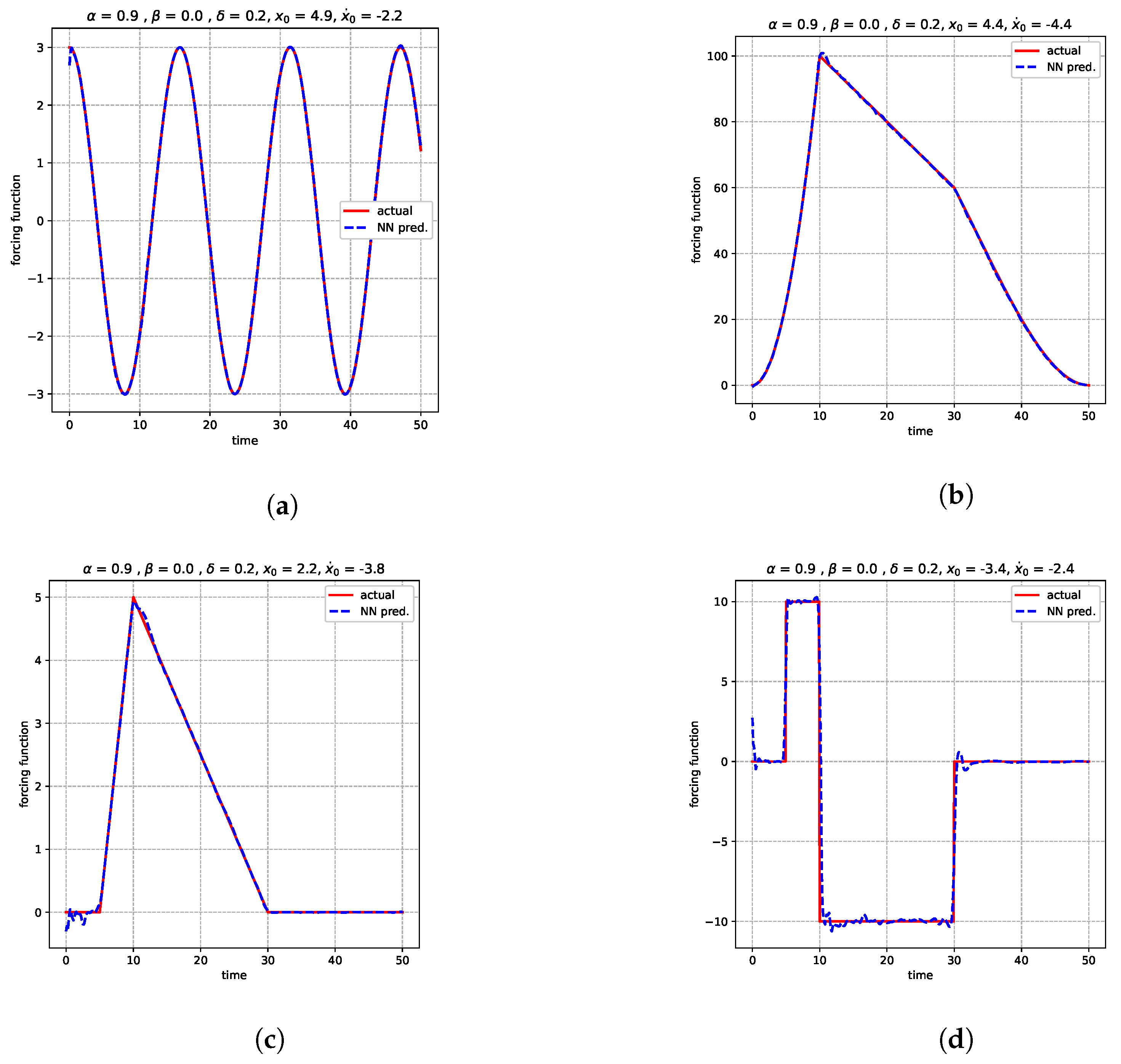
In Section 4 we shared our findings that demonstrated the effectiveness of our proposed neural network approach for solving the inverse source problem of dynamic load identification by incorporating physics information. The neural network structure and best working hyper-parameter choices were obtained by performing systematic hyper-parameter tuning. The network was later trained on different data instances generated by simulating spring mass damper systems subjected to different types of forcing functions, including smooth, abrupt changes in gradient, and jump discontinuities.

The neural network predictions in all cases were excellent, with slight overshoot and undershoot at the cusp of both piece-wise functions and some small oscillations at the start of the triangular function. However, some numerical oscillations were observed in step function predictions that resemble the Gibbs phenomenon. The findings suggest that the proposed neural network approach was effective in predicting different types of forcing functions.

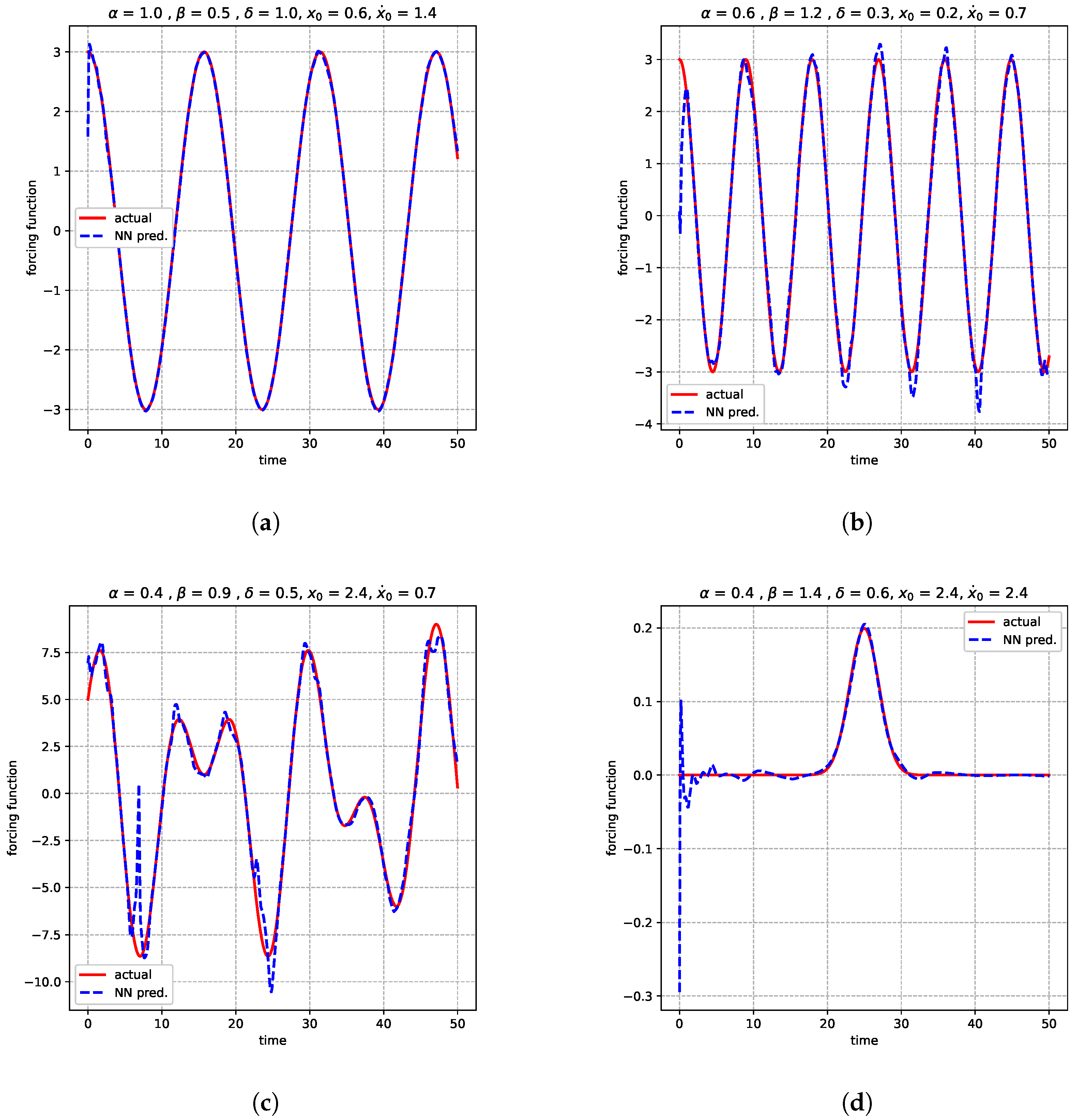
The study also tested the network to recover the forcing functions of non-linear oscillators from the data. The data were generated by solving duffing equations subjected to various smooth forcing functions. The network was able to predict sinusoidal functions and sinusoidal functions with increased non-linearity and frequency with small amounts of instability and minor overshoot and undershoot at the peak and trough of the periodic function.

Finally, the network was used to predict functions given by the sum of two sinusoidal functions and an impulse, and the network prediction was in close agreement with the actual function. However, some under and over-predictions with small oscillations were observed at the peaks and valleys of the functions in the case of the sum of two sinusoidal functions. In the case of a forcing function involving an impulse, numerical oscillations were observed at the start that dampened out in the later stages of predictions.

Overall, the findings of this study demonstrate that the proposed technique works well in predicting a variety of forcing functions from response data, although, only smooth functions were considered in the case of non-linear oscillators. Additionally, the analysis was based on simulated data without any noise used to train the neural network. Future studies should investigate the effectiveness of this technique using real-world data with noise and compare its performance with other established techniques for dynamic load identification.

6. Conclusions

In this paper, we presented an approach for solving the dynamic load identification problem using neural networks and physics information. We started our analysis by testing the efficacy of our architecture in recovering the forcing functions of the spring mass damper system and finally extending it to non-linear oscillators.

In our analysis of the spring mass damper system, we trained our neural network to recover different types of functions from the data, and it was found that our network was able to seamlessly recover them without much difficulty. Later on, we tried the same for the non-linear ODEs. In the case of non-linear ODEs, we primarily focused on smooth functions, and it was observed that our method was able to recover almost all of the functions, but with minor numerical oscillations at different places.

Though this work was predominantly focused on predicting the source terms of ODEs with mechanical systems in mind, to the best of our understanding, this has the potential to be applied to any system where the interest is in finding the source term from response data.

In the future, this work can be extended by testing whether the architecture can recover discontinuous forcing functions of non-linear ODEs and if similar predictions can be made from data that are corrupted by noise. Also, a similar study can be undertaken for recovering both smooth and discontinuous forcing functions in a multi-degree of freedom system. Another possibility is to test if our neural network architecture can predict the forcing function just from one set of data, i.e., displacement or velocity.

Finally, this work was focused on recovering the forcing function of a specific ODE from its data instances. However, a surrogate model can also be developed that can be trained on huge sets of data and, after training, can predict the forcing function for any instance of a linear or non-linear ODE from its response time histories and initial conditions.

References

1. Kabanikhin, S.I. Definitions and examples of inverse and ill-posed problems. J. Inverse Ill-Posed Probl. 2008, 16, 317–357. Available online: https://www.degruyter.com/document/doi/10.1515/JIIP.2008.019/html (accessed on 9 March 2023). [CrossRef]
2. Sabatier, P.C. Past and future of inverse problems. J. Math. Phys. 2000, 41, 4082–4124. [Google Scholar] [CrossRef]
3. Yaman, F.; Yakhno, V.G.; Potthast, R. A Survey on Inverse Problems for Applied Sciences. Math. Probl. Eng. 2013, 2013, 976837. [Google Scholar] [CrossRef]
4. Uhlmann, G.; Uhlmann, S.G.F. Inverse problems: Seeing the unseen. Bull. Math. Sci. 2014, 4, 209–279. [Google Scholar] [CrossRef]
5. McCormick, N.J. Inverse Radiative Transfer Problems: A Review. Nucl. Sci. Eng. 2017, 112, 185–198. [Google Scholar] [CrossRef]
6. Stefanov, P.; Uhlmann, G. An inverse source problem in optical molecular imaging an inverse source problem in optical molecular imaging. Anal. PDE 2008, 1, 115–116. [Google Scholar] [CrossRef]
7. Ammari, H.; Bao, G.; Fleming, J.L. An Inverse Source Problem for Maxwell’s Equations in Magnetoencephalography. SIAM J. Appl. Math. 2006, 62, 1369–1382. [Google Scholar] [CrossRef]
8. Grech, R.; Cassar, T.; Muscat, J.; Camilleri, K.P.; Fabri, S.G.; Zervakis, M.; Xanthopoulos, P.; Sakkalis, V.; Vanrumste, B. Review on solving the inverse problem in EEG source analysis. J. NeuroEng. Rehabil. 2008, 5, 25. [Google Scholar] [CrossRef]
9. Huang, C.H. A generalized inverse force vibration problem for simultaneously estimating the time-dependent external forces. Appl. Math. Model. 2005, 29, 1022–1039. [Google Scholar] [CrossRef]
10. Ma, C.K.; Tuan, P.C.; Lin, D.C.; Liu, C.S. A study of an inverse method for the estimation of impulsive loads. Int. J. Syst. Sci. 1998, 29, 663–672. [Google Scholar] [CrossRef]
11. Azam, S.E.; Chatzi, E.; Papadimitriou, C. A dual Kalman filter approach for state estimation via output-only acceleration measurements. Mech. Syst. Signal Process. 2015, 60, 866–886. [Google Scholar] [CrossRef]
12. Jang, T.S.; Baek, H.; Choi, H.S.; Lee, S.G. A new method for measuring nonharmonic periodic excitation forces in nonlinear damped systems. Mech. Syst. Signal Process. 2011, 25, 2219–2228. [Google Scholar] [CrossRef]
13. Feldman, M. Mapping nonlinear forces with congruent vibration functions. Mech. Syst. Signal Process. 2013, 37, 315–337. [Google Scholar] [CrossRef]
14. Chao, M.; Hongxing, H.; Feng, X. The identification of external forces for a nonlinear vibration system in frequency domain. Proc. Inst. Mech. Eng. Part C J. Mech. Eng. Sci. 2014, 228, 1531–1539. [Google Scholar] [CrossRef]
15. Liu, C.S.; Chang, C.W. A real-time Lie-group differential algebraic equations method to solve the inverse nonlinear vibration problems. Inverse Probl. Sci. Eng. 2016, 24, 1569–1586. [Google Scholar] [CrossRef]
16. Rice, C.; Frankel, J.I. Estimating the forcing function in a mechanical system by an inverse calibration method. JVC/J. Vib. Control 2022, 28, 3352–3363. [Google Scholar] [CrossRef]
17. Liu, R.; Dobriban, E.; Hou, Z.; Qian, K. Dynamic Load Identification for Mechanical Systems: A Review. Arch. Comput. Methods Eng. 2022, 29, 831–863. [Google Scholar] [CrossRef]
18. Prawin, J.; Rao, A.R.M. An online input force time history reconstruction algorithm using dynamic principal component analysis. Mech. Syst. Signal Process. 2018, 99, 516–533. [Google Scholar] [CrossRef]
19. Zhou, J.M.; Dong, L.; Guan, W.; Yan, J. Impact load identification of nonlinear structures using deep Recurrent Neural Network. Mech. Syst. Signal Process. 2019, 133, 106292. [Google Scholar] [CrossRef]
20. Yang, H.; Jiang, J.; Chen, G.; Mohamed, M.S.; Lu, F. A Recurrent Neural Network-Based Method for Dynamic Load Identification of Beam Structures. Materials 2021, 14, 7846. [Google Scholar] [CrossRef]
21. Rosafalco, L.; Manzoni, A.; Mariani, S.; Corigliano, A. An autoencoder-based deep learning approach for load identification in structural dynamics. Sensors 2021, 21, 4207. [Google Scholar] [CrossRef] [PubMed]
22. Liu, Y.; Wang, L.; Gu, K.; Li, M. Artificial Neural Network (ANN) - Bayesian Probability Framework (BPF) based method of dynamic force reconstruction under multi-source uncertainties. Knowl.-Based Syst. 2022, 237, 107796. [Google Scholar] [CrossRef]
23. Karniadakis, G.E.; Kevrekidis, I.G.; Lu, L.; Perdikaris, P.; Wang, S.; Yang, L. Physics-informed machine learning. Nat. Rev. Phys. 2021, 3, 422–440. [Google Scholar] [CrossRef]
24. Raissi, M.; Perdikaris, P.; Karniadakis, G.E. Physics-informed neural networks: A deep learning framework for solving forward and inverse problems involving nonlinear partial differential equations. J. Comput. Phys. 2019, 378, 686–707. [Google Scholar] [CrossRef]
25. He, Z.; Ni, F.; Wang, W.; Zhang, J. A physics-informed deep learning method for solving direct and inverse heat conduction problems of materials. Mater. Today Commun. 2021, 28, 102719. [Google Scholar] [CrossRef]
26. Liu, Q.; Zhao, Z.; Zhang, Y.; Wang, J.; Cao, J. Physics-informed sparse identification of bistable structures. J. Phys. D Appl. Phys. 2022, 56, 044005. [Google Scholar] [CrossRef]
27. Haghighat, E.; Bekar, A.C.; Madenci, E.; Juanes, R. Deep learning for solution and inversion of structural mechanics and vibrations. Model. Comput. Vib. Probl. 2021, 1, 1–17. [Google Scholar] [CrossRef]
28. Antonio, D.; Zanette, D.H.; López, D. Frequency stabilization in nonlinear micromechanical oscillators. Nat. Commun. 2012, 3, 806. [Google Scholar] [CrossRef]
29. Lim, F.; Cartmell, M.; Cardoni, A.; Lucas, M. A preliminary investigation into optimising the response of vibrating systems used for ultrasonic cutting. J. Sound Vib. 2004, 272, 1047–1069. [Google Scholar] [CrossRef]
30. Cao, Q.; Xiong, Y.; Wiercigroch, M. A novel model of dipteran flight mechanism. Int. J. Dyn. Control 2013, 1, 1–11. [Google Scholar] [CrossRef]
31. Kovacic, I.; Brennan, M.J. The Duffing Equation: Nonlinear Oscillators and Their Behaviour; John Wiley & Sons: Hoboken, NJ, USA, 2011. [Google Scholar]
32. Abadi, M.; Agarwal, A.; Barham, P.; Brevdo, E.; Chen, Z.; Citro, C.; Corrado, G.S.; Davis, A.; Dean, J.; Devin, M.; et al. TensorFlow: Large-Scale Machine Learning on Heterogeneous Systems. 2015. Available online: tensorflow.org (accessed on 8 May 2023).
33. Chollet, F. Keras. 2015. Available online: https://keras.io (accessed on 9 March 2023).
34. Kingma, D.P.; Ba, J.L. Adam: A method for stochastic optimization. arXiv 2014, arXiv:1412.6980. [Google Scholar]
35. MATLAB, 9.8.0.1873465 (R2020a) Update 8’; The MathWorks Inc.: Natick, MA, USA, 2020.
Figure 1. Proposed neural network architecture with input t and output x ^ , x ˙ ^ and f ^ .
Algorithms 16 00250 g001
Figure 2. (ac) shows the total, data, and physics loss w.r.t the training epochs for one training instance.
Algorithms 16 00250 g002
Figure 3. Figure shows the training sample that was obtained by simulating Equation (1) by setting α = 0.4 , β = 0.9 , δ = 0.5 with initial conditions x 0 = 2.4 , x ˙ 0 = 0.7 subjected to forcing function given by Equation (14) with γ 1 = 5 , γ 2 = 4 , ω 1 = 0.4 , ω 2 = 0.7 .
Algorithms 16 00250 g003
Figure 4. Figure shows the agreement between neural network predictions and actual forcing functions: (a) sinusoidal (b) sinusoidal with increased non-linearity and frequency (c) sum of two sinusoidal (d) impulse for duffing’s equation.
Algorithms 16 00250 g004
Figure 5. Figure shows the agreement between neural network predictions and actual forcing functions: (a) sinusoidal (b) combination of parabolic, linear and cubic (c) triangular (d) step for spring mass damper system.
Algorithms 16 00250 g005
Disclaimer/Publisher’s Note: The statements, opinions and data contained in all publications are solely those of the individual author(s) and contributor(s) and not of MDPI and/or the editor(s). MDPI and/or the editor(s) disclaim responsibility for any injury to people or property resulting from any ideas, methods, instructions or products referred to in the content.