Well-Separated Pair Decompositions for High-Dimensional Datasets

Abstract

Well-separated pair decomposition (WSPD) is a well known geometric decomposition used for encoding distances, introduced in a seminal paper by Paul B. Callahan and S. Rao Kosaraju in 1995. WSPD compresses $O\left(n^2\right)$ pairwise distances of n given points from ${\mathbb{R}}^d$ in $O\left(n\right)$ space for a fixed dimension d. However, the main problem with this remarkable decomposition is the “hidden” dependence on the dimension d, which in practice does not allow for the computation of a WSPD for any dimension $d>2$ or $d>3$ at best. In this work, I will show how to compute a WSPD for points in ${\mathbb{R}}^d$ and for any dimension d. Instead of computing a WSPD directly in ${\mathbb{R}}^d$, I propose to learn nonlinear mapping and transform the data to a lower-dimensional space ${\mathbb{R}}^{d^{\prime }}$, $d^{\prime }=2$ or $d^{\prime }=3$, since only in such low-dimensional spaces can a WSPD be efficiently computed. Furthermore, I estimate the quality of the computed WSPD in the original $R^d$ space. My experiments show that for different synthetic and real-world datasets my approach allows that a WSPD of size $O\left(n\right)$ can still be computed for points in ${\mathbb{R}}^d$ for dimensions d much larger than two or three in practice.

1. Introduction

Given a set of points $S\subset {\mathbb{R}}^d$, $\left|S\right|=n$, a well-separated pair decomposition (WSPD) can be seen as a compressed representation for approximating $\left(\genfrac{}{}{0pt}{}{n}{2}\right)$ pairwise distances of n points from S into $O\left(n\right)$ space, where the dimension d is considered a constant. The formal definition of a WSPD will be given in Section 2. A WSPD can also be seen as a clustering approach, e.g., a WSPD is a partition of the $\left(\genfrac{}{}{0pt}{}{n}{2}\right)$ edges of the complete Euclidean graph into $O\left(n\right)$ subsets. This decomposition was first introduced in a seminal paper [1] by Paul B. Callahan and S. Rao Kosaraju in 1995. It has been shown in [1] that the size of a WSPD, when computed by their algorithm, is exponential in d. Hence, it has never been used in practice for dimensions larger than three.

However, a WSPD has been shown to be useful in many different applications. It is known that a WSPD can be used to efficiently solve a number of proximity problems [2], such as the closest pair problem, the all-nearest neighbors problem, etc. It is also known that a WSPD directly induces a t-spanner of a point set or provides a $(1+\epsilon )$ —approximation of the Euclidean minimum spanning tree. The authors in [3] used a WSPD to compute approximate energy-efficient paths in radio networks. Their algorithm reduced the complexity of computing such paths to $O\left(1\right)$ by moving most of the computation to the preprocessing stage by precomputing a template path for each pair of sets compressing the pairwise distances.

Since a WSPD proved to be an essential decomposition for different important problems, in this paper, I investigate to what extent a WSPD can be helpful for situations where the input $S\subset {\mathbb{R}}^d$ and the dimension d is much larger than two or three.

On the technical side, a WSPD of a set of points $S\subset {\mathbb{R}}^d$ is represented by a sequence of pairs of sets $(A_i,B_i)$, $i=1,\dots ,k$, called dumbbells, such that (i) for every two distinct points $a,b\in S$ there exists a unique dumbbell $(A_i,B_i)$ such that $a\in A_i,b\in B_i$; (ii) the distances between points in $A_i$ and $B_i$ are approximately equal; (iii) the distances between points in $A_i$ or points in $B_i$ are much smaller than the distances between points in $A_i$ and $B_i$.

As stated before, the size of a WSPD, i.e., the number of dumbbells, is known to grow exponentially with the dimension d. Hence, instead of computing a WSPD directly on $S\subset {\mathbb{R}}^d$, I first propose to transform the points in S with a nonlinear function $f_{\theta }:{\mathbb{R}}^d\to {\mathbb{R}}^{d^{\prime }}$, $d^{\prime }=2$ or $d^{\prime }=3$, where $\theta$ denotes the set of learnable function parameters. The parameters $\theta$ are determined such that the function $f_{\theta }$ preserves the properties of S that are important for a WSPD, e.g., preserves pairwise distances for points in S. If the function $f_{\theta }$ manages to preserve most of the important information for a WSPD, there is hope that the WSPD computed on the mapped points $f_{\theta }\left(S\right)\subset {\mathbb{R}}^{d^{\prime }}$, $d^{\prime }=2$ or $d^{\prime }=3$, where the size of the WSPD is $O\left(n\right)$, will output “dumbbells” that are meaningful even for the original input S. If this is the case, the reconstructed dumbbells should continue to be “dumbbell-shaped” in the original space. In practice, some of the reconstructed dumbbells can become “bad” because they do not approximate the distances in any practical sense. However, I will show that the number of “bad” dumbbells is negligible in practice. Moreover, such “bad” dumbbells can be easily refined without significantly increasing the total number of dumbbells. One tool I employ might be of independent interest: I implemented a WSPD following the nontrivial algorithm of the partial fair-split tree that guarantees the construction time of $O(nlogn)$ and a WSPD of $O\left(n\right)$ size. To my knowledge, my implementation is the first open-source publicly available implementation of a WSPD that carefully follows the original algorithm in [1]. The implementation of a WSPD in the ParGeo C++ library (see [4]) uses a simple fair-split kd-tree and as such does not ensure theoretical bounds on the size of a WSPD.

Recently, there have been attempts to improve classical clustering for high-dimensional datasets. The authors in [5] have proposed a deep embedded clustering method that simultaneously learns feature representations and cluster assignments using a nonlinear mapper $f_{\theta }$. The work of [6,7] proposed an interesting Maximal Coding Rate Reduction principle for determining the parameters $\theta$ of the function $f_{\theta }$. The work of [8] further developed that idea in the context of manifold clustering.

Although this work was motivated by the research above, I note that their use of a function $f_{\theta }$ was aimed at improving clustering in the sense that a nonlinear mapper $f_{\theta }$ was used as an additional mechanism to “learn” a better set of features that would enable a better clustering. In my approach, $f_{\theta }$, which is represented by a neural network, is primarily used as a mapper to a very low-dimensional representation of the original dataset, since only there can a WSPD be computed efficiently.

In the rest of this paper, I will formally define a WSPD and state two important theorems. Furthermore, I will introduce two different functions for $f_{\theta }$ and present steps for computing a WSPD for high-dimensional data sets. Finally, I provide empirical evidence for the claim that a WSPD of size $O\left(n\right)$ can be computed efficiently for dimensions d much larger than three.

2. Preliminaries

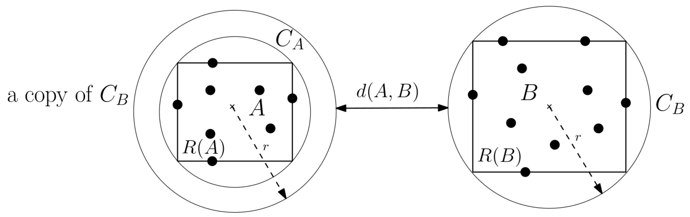
Let S be a set of n points in $R^d$. For any $A\subseteq S$, let $R\left(A\right)$ denote the minimum enclosing axis-aligned box of A. Let $C_A$ be the minimum enclosing ball of $R\left(A\right)$, and let $r\left(A\right)$ denote the radius of $C_A$. Let $C_A^r$ be the ball with the same center as $C_A$ but with radius r. Furthermore, for two sets A, $B\subseteq S$, let $r=max\left(r\right(A),r(B\left)\right)$, and let $d(A,B)$ denote the minimum distance between $C_A^r$ and $C_B^r$. For example, if the $C_A$ intersects $C_B$, then $d(A,B)=0$ (Figure 1).

Definition 1. 

A pair of sets A and B are said to be well separated (a dumbbell) if $d(A,B)>s·r$, for any given separation constant $s>0$ and $r=max\left\{r\right(A),r(B\left)\right\}$.

Definition 2 

(WSPD). A well-separated pair decomposition of $S\subset {\mathbb{R}}^d$, for a given $s>0$, is a sequence $(A_1,B_1),\dots ,(A_k,B_k)$, where $A_i,B_i\subseteq S$, such that the following applies:

1.

$A_i,B_i$ are well separated with respect to separation constant s, for all $i=1,\dots ,k$;

2.

For all $p\ne q\in S$, there exists a unique pair $(A_i,B_i)$ such that $p\in A_i,q\in B_i$ or $q\in A_i,p\in B_i$.

Note that a WSPD always exists since one could use all singleton pairs $\left(\right\{p\left\}\right\{q\left\}\right)$, for all pairs $p,q\in S$. However, this would yield a sequence of dumbbells of size $k=\Theta \left(n^2\right)$. The question is whether one could do better than that. The answer to that question was given by the following theorem.

Theorem 1 

([1]). Given a set S of n points in ${\mathbb{R}}^d$ and a separation constant $s>0$, a WSPD of S with $O\left(s^d{d}^{d/2}n\right)$ amount of dumbbells can be computed in $O(dnlogn+s^d{d}^{d/2}n)$ time.

While Theorem 1 states that it is possible to compute only $O\left(n\right)$ dumbbells, for fixed dimension d, it is still not clear how to efficiently determine the appropriate dumbbell for a given query pair $(p,q)$. In [3], it has been shown that retrieving the corresponding dumbbell can be performed in $O\left(1\right)$ time for a fixed dimension d.

Theorem 2 

([3]). Given a well-separated pair decomposition of a point set S with separation constant $s>2$ and fixed dimension d, I can construct a data structure in space $O(n·s^2)$ and construction time $O(n·s^2)$ such that for any pair of points $(p,q)$ in S I can determine the unique pair of clusters $(A,B)$ that is part of the well-separated pair decomposition with $p\in A,q\in B$ in constant time.

3. Deep Embedded WSPD

Instead of computing a WSPD of $S\subset {\mathbb{R}}^d$, as suggested by Theorem 1, I propose to first transform the data with a nonlinear mapping $f_{\theta }:R^d\to R^{d^{\prime }}$, where $d^{\prime }$ is chosen to be either 2 or 3, and $\theta$ is a set of learnable parameters. In this section, I introduce two approaches for training the neural net for embedding the point sets.

3.1. Metric Multidimensional Scaling

The most natural choice for a function $f_{\theta }$ is to use metric multidimensional scaling (mMDS), which tries to preserve the pairwise distances between points, i.e., it solves the optimization problem

$$\underset{\theta }{min}\sum _{i,j}{w}_{ij}\left(\right||x_i-x_j\left|\right|-\left|\right|f_{\theta }\left(x_i\right)-f_{\theta }\left(x_j\right){\left|\right|)}^2,$$

(1)

where $\left|\right|·\left|\right|$ denotes the Euclidean norm and $w_{ij}\ge 0$ are some given weights. For the implementation of a function $f_{\theta }$, I will use deep neural networks. The neural network approach for computing the metric MDS mapper has already been used in [9]. Inspired by the work of  [5,10,11], I chose the following architecture with $L=$ five fully connected layers of the form below:

$$d-500-500-2000-d^{\prime }$$

and $d^{\prime }\in \{2,3\}$. Moreover, the output $h_k^x$, $k>1$ of the kth layer for each $x\in S$ is defined as follows:

$$h_k^x=g(W_{k-1}{h}_{k-1}^x+b_{k-1})$$

(2)

where $h_1^x$ is just another name for any $x\in S$, $g(·)$ denotes an activation function and $\theta =\{W_k,b_k|k=1,\dots ,L-1\}$ are model parameters. For the activation function $g(·)$, I use the hyperbolic tangent (tanh).

3.2. Autoencoder

We will also implement the function $f_{\theta }$ as a stacked autoencoder, a type of neural network typically used to learn encodings of unlabeled data. It is known that such a learned data representation maintains semantically meaningful information ([12,13]). Moreover, it has been shown in [14], one of the seminal papers in deep learning, that an autoencoder can be effectively used on real-world datasets as a nonlinear generalization of the widely used principal component analysis (PCA).

The fundamental concept is to use an encoder to reduce high-dimensional data to a low-dimensional space. However, this results in a loss of information in the data. The decoder then works to map the data back to its original space. The better the mapping, the less information is lost in the process. Thus, the basic idea of an autoencoder is to have an output layer with the same dimensionality as the inputs. In contrast, the number of units in the middle layer is typically much smaller compared to the inputs or outputs. Therefore, it is assumed that the middle layer units contain a reduced data representation. Since the output is supposed to approximate the input, it is hoped that the reduced representation preserves “interesting” properties of the input (e.g., pairwise distances). It is common that autoencoders have a symmetric architecture, i.e., for an odd number L, the number of units in the kth layer of an L-layer autoencoder architecture is equal to the number of units in the $(L-k+1)$th layer. Moreover, the first part of the network, up to the middle layer, is called the encoder, while the part from the middle layer to the outputs is called the decoder.

We use a very similar architecture as above, namely $L=$ nine layers of the form below:

$$d-500-500-2000-d^{\prime }-2000-500-500-d$$

for $d^{\prime }\in \{2,3\}$. The output $h_k^x$, $k>1$ of the kth layer for any $x\in S$ is computed as above using the tanh activation function. Training is conducted by minimizing the following least squares loss:

$$\underset{\theta }{min}\sum _{x\in S}\left|\right|x-h_L^x{\left|\right|}^2.$$

(3)

Once the autoencoder is trained on a given dataset S, the encoder part of the network $d-500-500-2000-d^{\prime }$ is used as a nonlinear mapper $f_{\theta }:{\mathbb{R}}^d\to {\mathbb{R}}^{d^{\prime }}$, and the decoder part is discarded.

3.3. Computing WSPD in High Dimensions

Given a function $f_{\theta }$, the algorithm for computing a WSPD of a high-dimensional dataset $S\subset {\mathbb{R}}^d$ is given by the following steps:

• Compute a lower-dimensional representation $S^{\prime }=f_{\theta }\left(S\right)$.
• Compute a WSPD$(S^{\prime },s)$, for any given $s>0$, as proposed by Theorem 1. Let $(A_i^{\prime },B_i^{\prime })$, $i=1,\dots ,k$, denote the dumbbells.
• Reconstruct $(A_i,B_i)$, $i=1,\dots ,k$, in the original ${\mathbb{R}}^d$ space. Note that not all of them are well separated, i.e., they are not dumbbells anymore.
• Refine all not well-separated pairs $(A_i,B_i)$ until they become dumbbells.

We will refer to the above steps as the NN-WSPD algorithm. Note that the reconstruction step in NN-WSPD can be performed efficiently. What requires further explanation is the refine step, which guarantees that the set of computed dumbbells in ${\mathbb{R}}^d$ is in fact again a well separated pair decomposition of S. Suppose $(A_i,B_i)$ for some i is not well separated and let $r\left(B_i\right)>r\left(A_i\right)$. We propose the following steps in Algorithm 1 to refine $(A_i,B_i)$.

Algorithm 1 Refine($A_i$, $B_i$)

if $(A_i,B_i)$ is not a dumbbell then     Split $B_i$ into $B_i^{\prime }$ and $B_i^{″}$    ▹Assuming $r\left(B_i\right)>r\left(A_i\right)$, otherwise split $A_i$     Remove $(A_i,B_i)$ from WSPD.     Add $(A_i,B_i^{\prime })$ and $(A_i,B_i^{″})$ to WSPD     Refine($A_i$, $B_i^{\prime }$) and Refine($A_i,B_i^{″}$)           ▹(Two recursive calls) end if

The complexity of the refine step depends on the recursion depth. We will experimentally demonstrate that the depth is relatively small for all the datasets that I tried in practice, introducing just a moderate number of new dumbbells.

3.4. Fast Dumbbell Retrieval in High Dimensions

As Theorem 2 stated, for any pair of points $a,b\in S$ I can determine the unique dumbbell $(A,B)$, $a\in A,b\in B$, in constant time but only if dimension d is considered constant. The hidden constant in the running time is again exponential in d (due to the packing argument used in [3], Lemma 10). Hence, the only way for a pair of points $(a,b)\in S$ to retrieve the corresponding dumbbell $(A,B)$ efficiently is to build and query the data structure proposed in [3] in lower-dimensional representation ${\mathbb{R}}^{d^{\prime }},d^{\prime }=2,3$. Namely, let $(A_i^{\prime },B_i^{\prime }),i=1,\dots ,k^{\prime }$, denote the dumbbells in ${\mathbb{R}}^{d^{\prime }}$ and $(A_i,B_i),i=1,\dots ,k$, the reconstructed and refined dumbbells in ${\mathbb{R}}^d$ computed by NN-WSPD. Note that $k\ge k^{\prime }$ in general, since the number of reconstructed and refined dumbbells might be larger. However, let $(f_{\theta }\left(A_i\right),f_{\theta }\left(B_i\right))$, $i=1,\dots ,k$, denote the corresponding dumbbells in ${\mathbb{R}}^{d^{\prime }}$ of the WSPD computed by NN-WSPD in ${\mathbb{R}}^d$. Note that $(f_{\theta }\left(A_i\right),f_{\theta }\left(B_i\right))$, $i=1,\dots ,k$ is also a valid WSPD of $S^{\prime }=f_{\theta }\left(S\right)$, and let query$(·,·)$ denote the query call to the data structure proposed in [3] built on that WSPD. The query algorithm for any two points $(a,b)\in S\subset {\mathbb{R}}^d$ is defined in Algorithm 2.

Algorithm 2 RetrieveDumbbell(a, b)

Require:  $f_{\theta }$, $(f_{\theta }\left(A_i\right),f_{\theta }\left(B_i\right))$ for $i=1,\dots ,k$, query$(·,·)$  Let $a^{\prime }=f_{\theta }\left(a\right)$, $b^{\prime }=f_{\theta }\left(b\right)$  $(A^{\prime },B^{\prime })$ = query$(a^{\prime },b^{\prime })$       ▹ Retrieve dumbbells by query$(·,·)$ from [3]  Return $(A,B)$ such that $A^{\prime }=f_{\theta }\left(A\right),B^{\prime }=f_{\theta }\left(B\right)$

The run-time complexity of Algorithm 2 again depends on the number of additional dumbbells that the refine step will add.

4. Experiments

Our implementations of the neural networks are performed in PyTorch [15], and a WSPD is implemented in C++ following the algorithm proposed in [1]. All codes are available for testing at https://github.com/dmatijev/high_dim_wspd.git. The experiments were conducted on Ryzen 9 3900X, with 12 cores and 64GB of DDR4 RAM with an Ubuntu 20.04 operating system.

For the training of the neural networks, I use an initial learning rate of 0.001 and a batch size of 512. All networks are trained for a number of epochs set to 500. It is essential to state that I did not put effort into fine-tuning these hyperparameters. Instead, all hyperparameters are set to achieve a reasonably good WSPD reconstruction and, to maintain fairness, are held constant across all datasets. We used Adam [16] for first-order gradient-based optimization and the ReduceLROnPlateau callback for reducing the learning rate (dividing it by 10) when a metric, given by (1) for mMDS NN, and (3) in the case of autoencoder NN, has stopped improving.

4.1. Datasets

We evaluated the computation of a WSPD on artificially generated and real high-dimensional datasets. Artificially generated datasets are drawn from the following:

• A uniform distribution over the ${[0,1]}^d$ hypercube;
• A normal (Gaussian) distribution, with mean 0 and standard deviation 1;
• A Laplace or double exponential distribution, with the position of the distribution peak at 0 and the exponential decay at 1.

For real-world datasets, I used two public scRNA-seq datasets downloaded from [17]. scRNA-seq data are used to assess which genes are turned on in a cell and in what amount. Therefore, scRNA-data are typically used in computational biology to determine transcriptional similarities and differences within a population of cells, allowing for a better understanding of the biology of a cell. We apply the standard preprocessing to scRNA-seq data (see [18,19]): (a) compute the natural log-transformation of gene counts after adding a pseudo count of 1 and (b) select the top 2000 most variable genes followed by a dimensionality reduction to 100 principle components. We used two datasets of sizes $n=4185$ and $n=68,575$.

One possible motivation for a WSPD on scRNA-seq data can be found in the work of [20]. Namely, the authors in [20] solve the marker gene selection problem by solving a linear program (LP). For a large amount of data, the LP cannot be efficiently solved in practice. Hence, the practical approach to that issue could be to solve an LP on a subset of constraints, then define a separation oracle that iteratively introduces new constraints to the LP, if the current solution is not feasible. Following the work of [20], the oracle could add the currently most violated constraints, i.e., pairs of points whose distance is less than a predefined constant value. Given the WSPD, one could speed up the oracle by using dumbbells as a substitute for the pairwise distances.

4.2. Measuring the Quality of a WSPD

Let $(A_i,B_i)$, $i=1,\dots ,k$, denote the WSPD for some set of points $S\subset {\mathbb{R}}^d$. For $a,a^{\prime }\in A_i$ and $b,b^{\prime }\in B_i$ for some dumbbell i, I make the following observations:

• Points within the sets $A_i$ and $B_i$ can be made “arbitrarily close” as compared to points in the opposite sets by choosing the appropriate separation $s>0$, i.e.,

  $$d(a,a^{\prime })\le 2r<\frac{2}{s}d(A_i,B_i)\le \frac{2}{s}d(a,b).$$

  (4)
• Distances between points in the opposite sets can be made “almost equal”, by choosing the appropriate $s>0$, i.e.,

  $$d(a^{\prime },b^{\prime })\le d(a,a^{\prime })+d(a,b)+d(b,b^{\prime })<(1+\frac{4}{s})d(a,b).$$

  (5)

Since a WSPD is primarily concerned with compressing the quadratic space of pairwise distances into a linear space (for a fixed dimension d), I will use Equation (5) repeatedly in my plots in order to measure how much distances are indeed preserved within a dumbbell.

4.3. Results

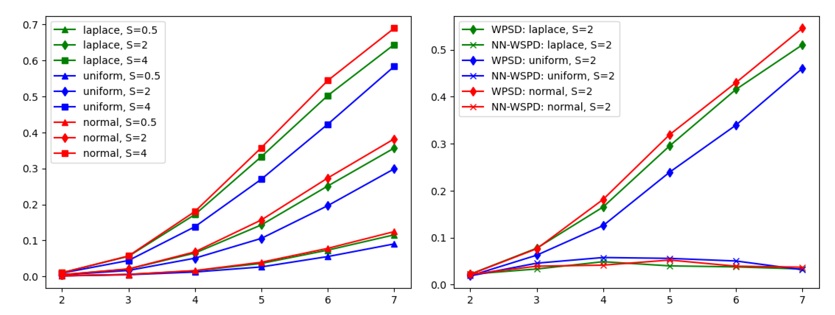
In Figure 2 (left), synthetic datasets were used to demonstrate the dependence between the size of a WSPD and the dimension of the input data in practice. Recall that the number of dumbbells is bounded above by $O\left(s^d{d}^{d/2}n\right)$ (Theorem 1). In my experiments, I found that the dependence on dimension d is indeed severe, making the WSPD algorithm proposed in [1] unusable in practice for dimensions $d>2$ or $d>3$. However, it is unclear whether the number of dumbbells is just an artifact of the construction of the WSPD algorithm or whether that number of dumbbells is indeed necessary to satisfy the properties of a WSPD given by Definition 2. Thus, Figure 2 (right) demonstrates the total number of dumbbells when computed with the algorithm proposed in [1] and compares it to the number of dumbbells computed with the NN-WSPD approach.

• Observation: For many practical datasets, there exists a WSPD $(A_i,B_i)$, $i=1,\dots ,k$, with $k=O\left(n\right)$ for any dimension d, i.e., the hidden constant in $O(·)$ notation is not exponential in the dimension d.

I performed numerous experiments with synthetic data and my two real datasets to support my claim.

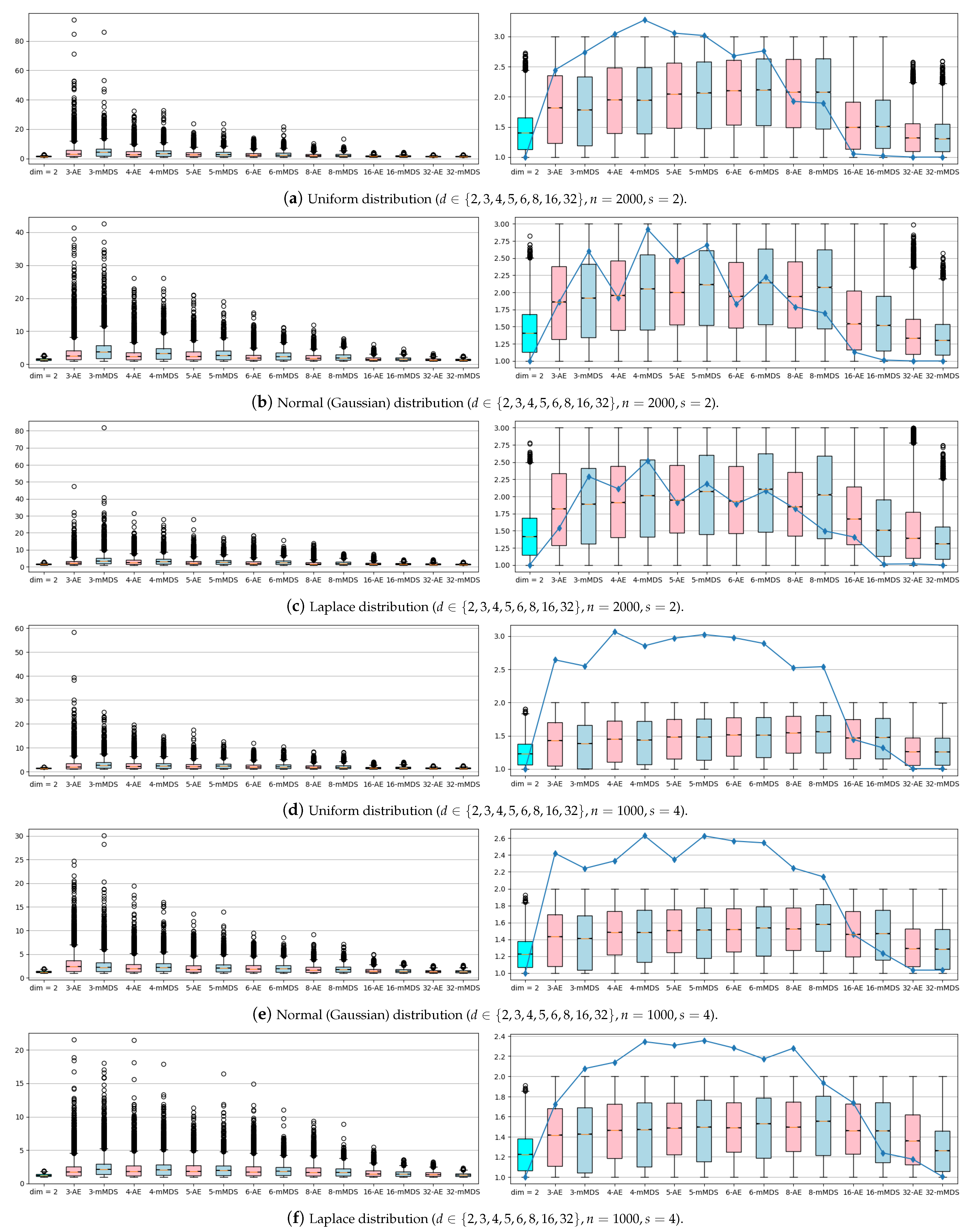
4.3.1. Synthetic Datasets

In Figure 3, the experiments were performed with the synthetic datasets. Only for $d=2$ was the standard WSPD algorithm used, and for $d>2$, NN-WSPD was used. On the boxplots in the left column, NN-WSPD was applied but without the refine step (Algorithm 1). From this one can see that many of the reconstructed dumbbells can violate the quality given by Equation (5), which the dumbbells are supposed to guarantee. However, most dumbbells are still well separated since a lot of valuable information for a WSPD was preserved by the nonlinear mapper $f_{\theta }$. The results of the refine step (Algorithm 1) can be seen in boxplots in the right column in Figure 3. Note that after the refine step all dumbbells are indeed dumbbells (i.e., well separated), with the overall number of dumbbells that rarely gets larger than the starting WSPD size multiplied by a factor of at most three, independent of the dimension d. We noticed that the higher the dimension d of the input set S, the fewer refined dumbbells are needed. This is not that surprising bearing in mind the fact that when a Euclidean distance is defined using many coordinates there is less difference in the distances between different pairs of samples (see the curse of dimensionality phenomenon [21]).

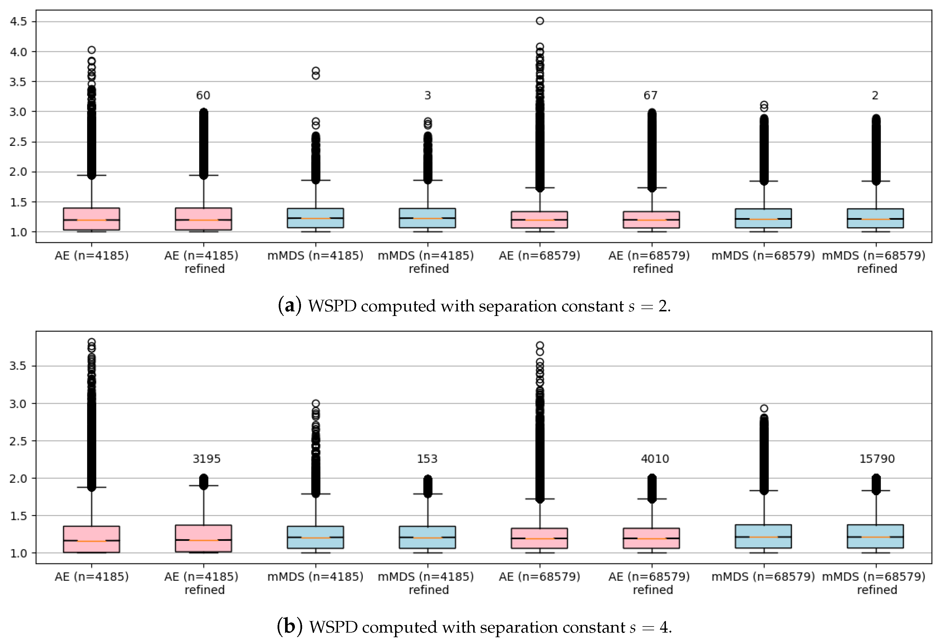
4.3.2. scRNA-Seq Datasets

I had even fewer problems computing a WSPD for my two real datasets ($n=4185$ and n = 68,579) that, after being preprocessed, were given in ${\mathbb{R}}^d$, $d=100$. In Figure 4, I output boxplots for both sets before and after the refining step. Note that the number of newly added refined dumbbells is negligible, even compared to the original sets’ size. Moreover, notice that computing a WSPD directly on such a high-dimensional input ($d=100$) is very inefficient and practically of no use due to the dependence on d. For example, I managed to compute a WSPD for dataset $n=4185$ in 507 s with 8,401,551 dumbbells, which is slightly above 95% of the overall size of pairwise distances, i.e., 95% of dumbbells were just singletone pairs $\left(\right\{a\},\{b\left\}\right)$. In contrast, my NN-WSPD approach always outputs a WSPD with a very moderate increase in size compared to a WSPD of size $O\left(n\right)$ computed in the plane the points were projected to, as my experiments showed.

5. Conclusions

Well-separated pair decomposition is a well known decomposition in computational geometry. However, computational geometry as a field is concerned with algorithms that solve problems on datasets in ${\mathbb{R}}^d$, where the dimension d is considered a constant. In this work, I demonstrated that a WSPD of size $O\left(n\right)$ could be computed even for high-dimensional sets, hence removing the requirement that dimension d is a constant. In my approach, I used an implementation of a nonlinear function $f_{\theta }$ that was based on artificial neural networks.

The past decade has seen remarkable advances in deep learning approaches based on artificial neural networks. We also witnessed a few successful applications of neural networks in discrete problems, e.g., I would like to point the reader to the surprising results presented in [22], which introduces a new neural network architecture (Ptr-Net) and shows that it can be used to learn approximate solutions to well-known geometric problems, such as planar convex hulls, Delaunay triangulations, and the planar traveling salesperson problem.

These advances inspire us to further explore the applications of deep learning in fields such as geometry.