Abstract
The justification for making a measurement can be sought in asking what decisions are based on measurement, such as in assessing the compliance of a quality characteristic of an entity in relation to a specification limit, SL. The relative performance of testing devices and classification algorithms used in assessing compliance is often evaluated using the venerable and ever popular receiver operating characteristic (ROC). However, the ROC tool has potentially all the limitations of classic test theory (CTT) such as the non-linearity, effects of ordinality and confounding task difficulty and instrument ability. These limitations, inherent and often unacknowledged when using the ROC tool, are tackled here for the first time with a modernised approach combining measurement system analysis (MSA) and item response theory (IRT), using data from pregnancy testing as an example. The new method of assessing device ability from separate Rasch IRT regressions for each axis of ROC curves is found to perform significantly better, with correlation coefficients with traditional area-under-curve metrics of at least 0.92 which exceeds that of linearised ROC plots, such as Linacre’s, and is recommended to replace other approaches for device assessment. The resulting improved measurement quality of each ROC curve achieved with this original approach should enable more reliable decision-making in conformity assessment in many scenarios, including machine learning, where its use as a metric for assessing classification algorithms has become almost indispensable.
1. Introduction
Few measurements are made solely for their own sake, and better justification for making a measurement can be sought by asking what decisions are to be taken based on the measurement. A typical decision of conformity is whether the attribute of an entity (e.g., a product or sample) can be classified as above (‘positive’) or below (‘negative’) a specification limit, SL, for that quality characteristic. Measurement uncertainty leads generally to the risk of incorrect decisions and classifications in such conformity assessments [1,2].
The so-called receiver operating characteristic (ROC) is a tool for assessing the performance of an instrument (e.g., a testing device or machine-learning algorithm) as part of a measurement system used for classification in a test of an entity in which “true positive rates” (TPR, sensitivity), plotted against decision risks such as “false positive rates” (FPR, fall-out), are made [3] (summarised in Appendix A).
Emerging from the radar rooms on board warships in the second world war [3], the ROC tool continues to gain popularity in many sectors and technologies. However, despite a burgeoning interest, little seems to have changed in how most ROC curves are evaluated in 80 years. In particular, the metrological quality assurance [4] of the ROC tool is difficult since limitations—an inherent non-linearity, the effects of ordinality [5] and a general confounding of task difficulty and instrument ability—are often unacknowledged, making ROC metrics for rating testing performance, such as area under curve (AUC), difficult and unreliable to interpret. This has much to do with the fact that ROC curves belong to classic test theory (CTT, Appendix A.1), whose limitations are becoming increasingly recognised in diverse fields such as psychometry, customer satisfaction studies and compositional data analysis [4]. As in those other fields, ROCs are expected to be prone to unnecessarily large uncertainties leading to substantial risks of incorrect decisions with potentially serious consequences in many fields of application.
These limitations in the venerable ROC tool, inherent and often unacknowledged, are tackled here for the first time with a modernised approach combining measurement system analysis (MSA) and item response theory (IRT). The performance of the new method of assessing device ability will be compared with previous ROC methodology, and recommendations will be made regarding replacing other approaches for device assessment.
The proposed methodology to modernise the ROC has general applicability. Examples include studies where the instrument-making classifications in support of diagnosis can either be a traditional engineering device (e.g., lateral flow assaying [6] such as pregnancy tests—as studied here—diabetes testing [7] and covid 19 screening tests [8]), or where a human acts as a measurement instrument [4], such as when the abilities of different clinicians to make correct diagnoses are to be assessed. ROC curves are also gaining popularity in modern technological areas such as machine learning, where their use as a metric for assessing machine learning algorithms has become almost indispensable [9].
Article Organistion
This work aims to demonstrate that many of the limitations inherent to traditional ROC curves (exemplified with the case of pregnancy testing in Section 3.1) can be tackled thanks to significant advances in the meantime in modern test theory, such as measurement system analysis (MSA, Section 3.2) and item response theory (IRT, Section 3.3), which have developed in parallel with the venerable ROC tool (Section 2).
The linearisation of ROC curves is a major part of the modernisation effort, together with MSA and IRT as proposed earlier (Section 3.4.1), and together with the new approach presented here (Section 3.4.2).
Section 4 contains the results of the application of the novel methods, presented in Section 3, to the pregnancy testing case study. The work culminates in Section 4.5 with an assessment of the functioning of the new metrics in comparison with more traditional metrics in judging the relative performance of devices, such as the popular area under curve metric (explained in Appendix A.1). Section 4 concludes with an appraisal of measurement uncertainties and limitations in the work so far.
The article closes with a discussion, some recommendations and a conclusion in Section 5.
2. Related Work
Traditional ROC curves have not been without their critics. It has been claimed that separate information about TPR (sensitivity) and FPR (1—specificity, fall-out) is lost in the making of an ROC plot, and no distinction is made for differences in device-specific SL [10]. As explained in Appendix A.1, better performing device types are considered to be those whose ROC curves lie furthest towards the left-hand, upper corner of the plots, but that procedure has been criticised as being only a relative judgment [3].
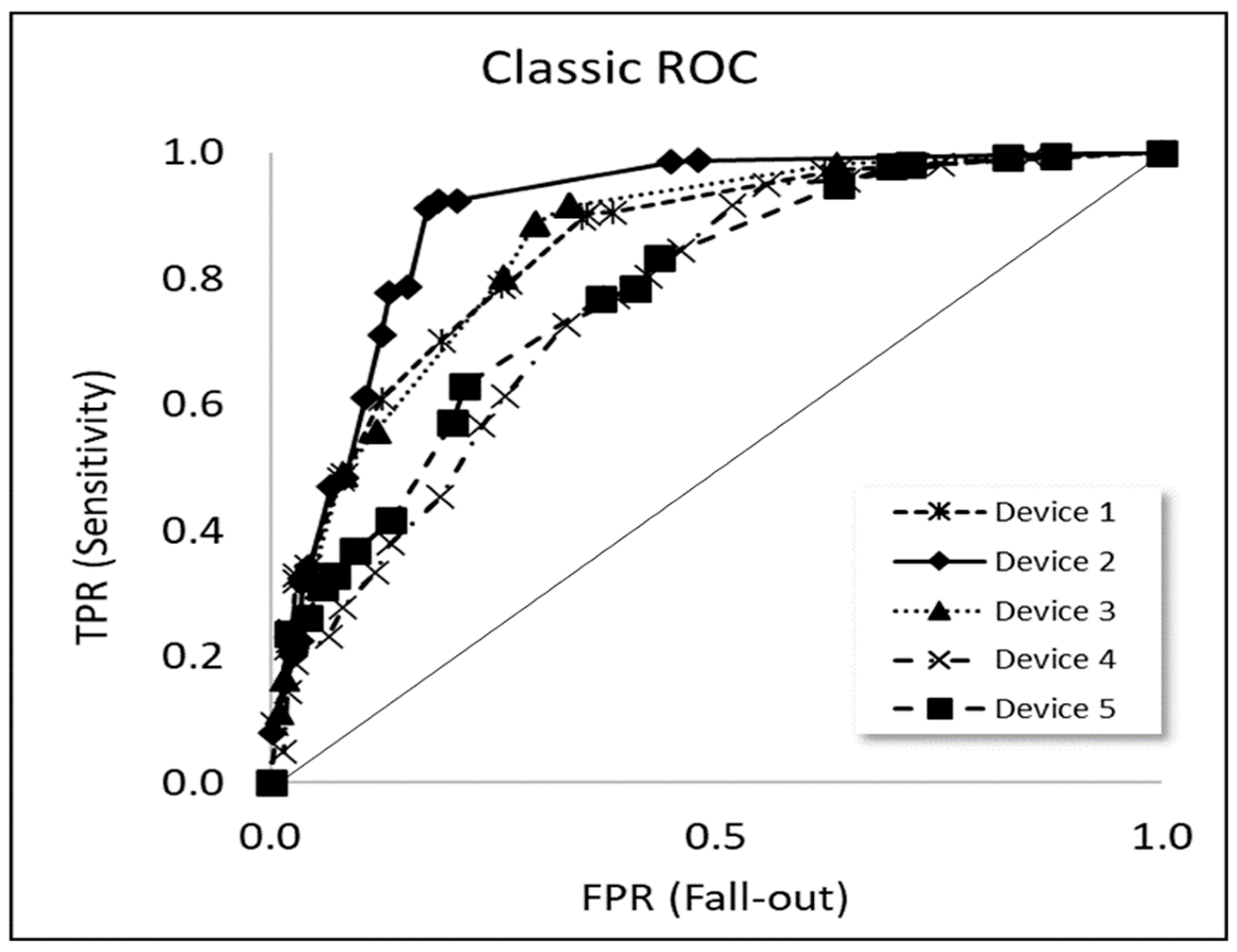
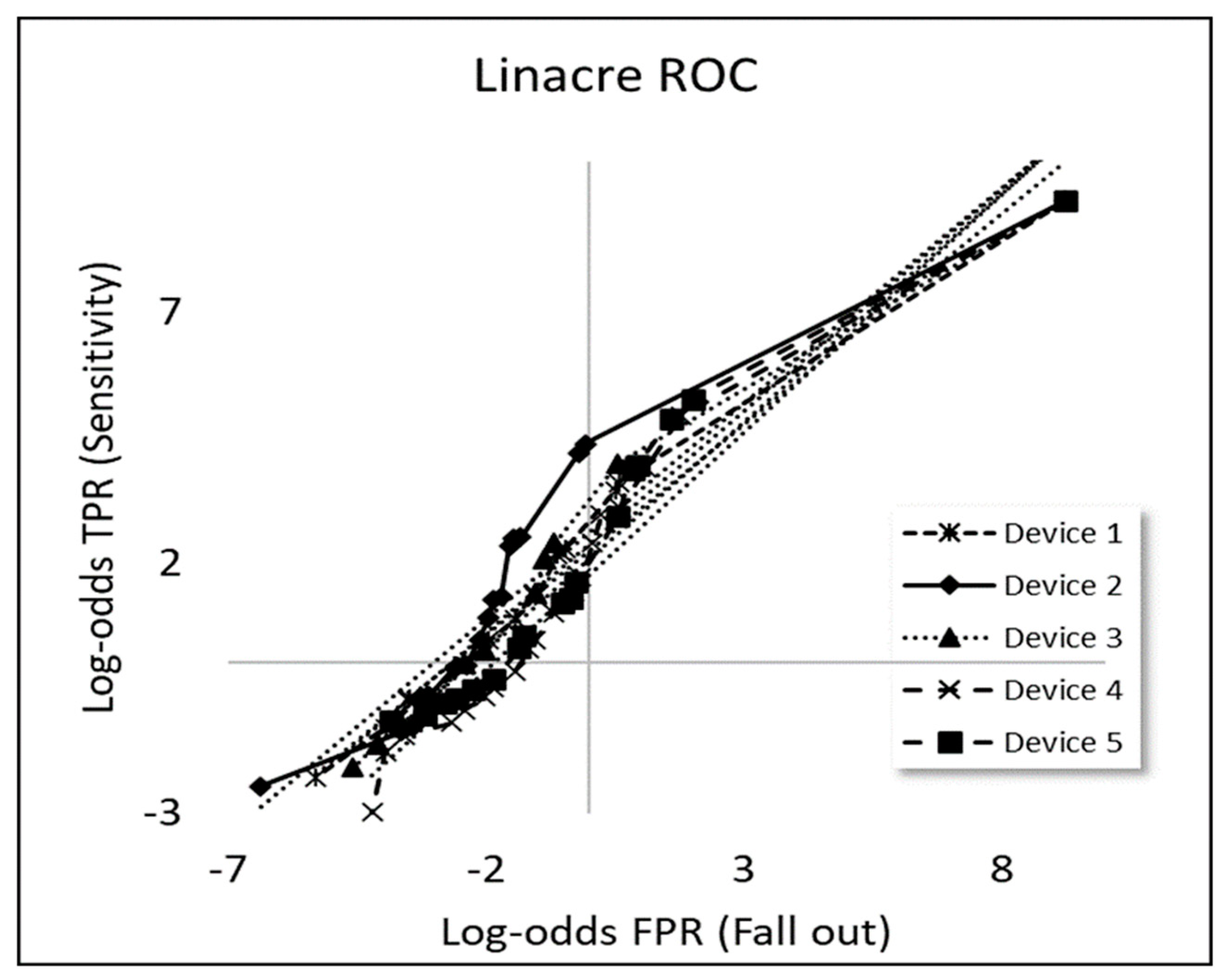
The limitations in interpretation due to the non-linearity of ROC curves have provoked, over the years, some suggestions about linearisation. For instance, early work by Birdsall [11] included the making of plots of ROC curves on log–log axes. Linacre [12] later proposed the linearisation of ROC curves by making plots of log-odds ratios (logits) on both plot axes instead of the non-linear % metrics TPR, FPR and AUC of traditional ROC curves (Figure 1), but Linacre apparently did not express these in terms of the Rasch model.

Figure 1.
Traditional ROC curves for the five device types used for pregnancy testing.
As explained in the introduction, much of that ROC work has been kept to CTT and many have been reluctant to adopt modern test theory (Section 1 and Appendix A.1), despite the latter’s development being concurrent with ROC use over the decades.
There has been some recent work which has included modern measurement theory, demonstrating improved diagnostic performance when Rasch-compensated metrics are used to plot traditional ROC curves. Cipriani et al. [13], for instance, considered the interpretations of standard ROC approaches with Rasch modelling, comparing test sensitivity, specificity, and likelihood ratios with the logit (and probability) estimates of the Rasch model, using the entire set of their available data (for the case of mechanical knee examinations). They demonstrated significant correlations between traditional approaches and Rasch model estimates and found that, for instance, positive likelihood ratios were significantly correlated with the probability values of a positive diagnosis from the Rasch model.
The diagnostic and demographic variables associated with the known differences in heart failure severity, with the potential for impacting the risk of intensive care unit admission, were included in another Rasch analysis by Fisher and Burton [14] intended as an aid in modelling the diagnostic process [13,15]. They compared ROC curves based on their unadjusted heart failure severity measures with ROC curves for the Rasch regression adjusted heart failure severity measures in which there is an improvement in AUC from 0.63 to 0.76, respectively, with the Rasch-adjusted measures. In a final comment, Fisher and Burton [14] mention that the Rasch regression concept [13,15] raises the possibility of using the log-odds ratios built into the heart failure severity measures (adjusted or unadjusted) as estimates of related outcome likelihoods.
In an even more recent work published during the writing of this manuscript, reference [16] reports on summary receiver operating characteristic (sROC) curves which are constructed using a regression model logit-TPR over logit-FPR.
Despite these recent advances, as far as we are aware, none of this recent work or others have explicitly addressed both of these limitations—i.e., counted fractions (Appendix A.1) and a lack of separation ability/difficulty (Appendix A.2)—and ROC curves have continued almost exclusively to be analysed in the traditional way.
3. Materials and Methods
As an illustration and case study of a modernised ROC methodology, we chose tests for pregnancy in order to exemplify the need for improved performance metrics and the establishment of performance goals for devices with binary responses (positive: hormone human choriogonadotropin (hCG) detected or negative: hCG not detected) in laboratory medicine. Pregnancy testing is chosen, not because it is particularly challenging, but rather because it is widely used and has many similarities with other binary classifications (see Introduction).
Single use devices for detecting the presence of a drug, hormone, or infectious agent in a sample are extensively used in health care, operated by both health care professionals and by lay people for self-testing. The measurement principle is often lateral flow immunoassay [6], in which the presence for a given substance above a certain concentration level is indicated by a shift in colour on the device display.
3.1. Traditional ROC Curves
A typical device for pregnancy testing, as studied here, is intended to give an early indication of pregnancy. The excretion of hCG in urine is well known as a marker for pregnancy based on a measurement of the level of hormone concentration, where a device is made to be responsive over the range of hormone concentration expected with pregnancy increasingly likely the higher the concentration.
In proficiency testing (external quality assessment) of the assays, samples with various concentrations of the substance are distributed to participants to regularly check their ability to perform measurement correctly, as well as the performance of the devices in themselves. For pregnancy testing, devices for the detection of the hormone hCG mostly have a stated specification limit, SL, of 25 IU/L [international units per litre].
Table 1 contains typical results. For a sample material containing 6 IU/L the expected major outcome for the devices is a negative result, when the SL is 25 IU/L. Users of device type 1 reported 91 (20%) positive results out of 451 measurements, and users of device type 3 reported 16 (6%) positive results out of 264 measurements. Table 1 is an extract of the raw data from our test sets covering the hormone concentration range . The first five rows show the five different device types in the present study for samples with the hCG concentration 6 IU/L and the five last rows shows device five for samples with five different hCG concentrations values.

Table 1.
Example of raw data (TPR and FPR as specified in Figure A1).
Examples of classic ROC curves, where TPR is plotted against FPR, based on our experimental proficiency testing data in the present case study, are shown in Figure 1 for five different types of urine test devices used for pregnancy testing.
Traditional ROC curves for device types used for pregnancy testing (such as those shown in Figure 1) are typically based on the classification task to detect the presence of hCG or not, as explained in Appendix A.1, and are given in the two last columns of Table 1 which are an extract from the complete dataset.
The ROC curves are produced by registering the binary response of each device: ‘hCG detected = positive’ or ‘hCG not detected = negative’. The original data covered distributions with assigned values in the concentration range 0 to 130 IU/L hCG, for five different device types in an external quality assessment scheme (proficiency testing) with four distributions per year for the period 2014–2021. We focused on the hormone concentration range from 6 IU/L hCG to 58 IU/L hCG, which covers the typical SL, and for the five most commonly used device types. A total of almost 19,000 responses across the 5 types of devices and range of hormone concentrations were investigated in this study.
A diagnosis of pregnancy is made, perhaps based on a typical SL of 25 IU/L hCG, which, of course, in the majority of cases can be confirmed by an actual pregnancy. Such observations can thus be used as ‘gold standard’ references for decision-making, for instance, in acting as diagnostic references for ROC curves when field devices such as those studied here are to be evaluated for performance. A limited product quality in pregnancy testing kits may lead to individual devices having cut-off values different from SL which, in turn, can lead to poorer measurement quality. A typical commercial device type often has a declared cut-off close in value to the diagnostic SL = 25 IU/L hCG, but with some uncertainty. Measurement uncertainty—as addressed further using MSA (Section 3.2) below—will also mean that risks of incorrect decisions are likely across the full range of concentration: false classifications of non-pregnancy (at concentrations above SL) and false classifications of pregnancy (at concentrations below SL).
3.2. Measurement System Analysis (MSA)
The ROC has mostly been used to date as a statistical tool, but here we also propose it to be a part of a measurement system analysis (MSA) when modernising the tool [4,17]. Employing an MSA approach allows ROC curves to be interpreted in terms of the performance metrics attributed to the different components of a measurement system which, for ROC, typically include the ability of a classifier (alternative MSA terms: ’agent’, ’person’, ’probe’, and so on) and the level of difficulty posed by the classification object (alternative MSA terms: ’task’, ‘item’, and so on), both of which can be entities that are individually subject to conformity assessment. Adopting an MSA approach brings to classification and decision-making analyses, including responses on ordinal and nominal scales, all the benefits of the substantial body of knowledge acquired over the decades in extensive studies, for example, in engineering measurement in manufacturing industries.
A first, all-important step in analysing any measurement situation with a view to quality assurance is to make as complete and correct description as possible of the actual measurement system used. A typical measurement system for the pregnancy testing studied here has, as a measurement object, the task of testing for pregnancy based on a hormone sample. The measurement instrument used to perform the task is a single-use device which senses the presence of the hCG hormone and gives a visual indication for a human operator of the level of concentration. As with similar tests, such as lateral flow COVID testing, the displayed response consists of a line, where the apparent intensity of the response line examined should be proportional to marker concentration. A binary decision is made by the operator by visually inspecting the appearance of the line. Measurement uncertainty may lead to, for instance, a faint response line which could be missed (or dismissed) leading to a false negative.
Such an MSA description provides invaluable support when identifying potential sources of measurement error, uncertainties, and the incorrect decisions they cause. Sources of measurement error can arise, for instance: at the measurement object level (such as variation of glycosylation and partial break-down of the hCG molecule between the distributed urine materials); at the instrument level (incorrect sample transfer and application to the device, variation in the content of chemical reagents and other properties of the single-use devices); and at the human operator level (mistaken interpretation of the response line, etc.). All of these elements can additionally be affected by the measurement environment and by the chosen measurement method. Traditional ROC curves arguably rarely consider MSA, even in modern applications such as in machine learning (Appendix A.1).
3.3. Item Response Theory (IRT) and the Rasch Model
Apart from MSA, a second part of renovating ROCs is the deployment of modern measurement theory which can address the special character of categorical-based measurements in a way not traditional in CTT. An observed response in a performance test is typically scored binarily in one of two categories: as for correct and for incorrect and presented as for each instrument, i, to a specific object, j. These observed responses constitute the raw data, , which cannot be analysed as regular quantitative data, but are characterised by ordinality, as explained in Appendix A. The responses are also not measures of the instrument’s ability, nor the task difficulty, but depend on both (see Appendix A.3).
A compensation for the ordinality of counted fractions (Appendix A.1) [4,5] and the provision of separate estimates of the quantities’ difficulty, , and ability, , attributed, respectively, to the object and instrument (Appendix A.2), are carried out in modern analyses by making a logistic regression with the Rasch modelling of the log-odds ratio to the raw binary response data, over all instruments, i, and objects, j [18]:
A detailed summary of the Rasch model and IRT is given in Appendix A.1, including comparing and contrasting with non-parametric and ranking tests still widely used in the field. A logistic regression of Equation (1) to the data can be readily performed with conventional software, such as WINSTEPS®3.80.1, RUMM2030, and different R-packages (e.g., eRM, tam, mirt). In this work, we calculate in two separate ways—see Section 3.4.2.
3.4. Modernising ROC
Here, we examine ROC curves in explicit terms of the Rasch model. As has been emphasised, firstly, not only are ROC curves technically more difficult to interpret than straight lines [12], they are also affected by counted fraction ordinality (Appendix A.1) and, secondly, the response probabilities in general confound the level of difficulty of the classification task and the ability of the classifier to make a correct classification (Appendix A.2). Thus, traditional ROC curves belong to classical test theory (CTT) while better approaches, including the Rasch approach and IRT as part of generalised linear modelling (GLM) have been known for a long time but, paradoxically, their up-take remains strikingly low.
3.4.1. Linacre Linearisation
Linacre’s [12] approach (Section 2) produces linearised ROC as correspondingly straight lines of slope and intercept according to the equation: evaluated for each device type (Figure 2; Table 2). As such, Linacre’s log-odds approach should take account to some extent of the effects of counted fractions (Appendix A.1).
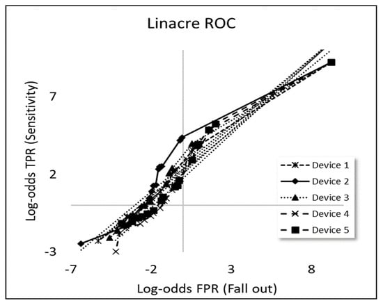
Figure 2.
A linearisation of the ROC curves (shown in Figure 1) by making linearised ROC plots of log-odds ratios according to the methodology proposed by Linacre [12]. (The dotted lines indicate linear regressions to each curve).

Table 2.
Experimental values of slope M and intercept C for linearised ROC curves in Figure 2, as proposed by Linacre [12]. Pearson correlation coefficient 0.97.
3.4.2. Linearised ROC Curves Adopting the Rasch Model
In this work, as reported in Section 4, we have extended Linacre’s [12] approach by, for each axis of the linearised ROC curves separately, adopting the Rasch model. As a first step, we made logistic regressions, using WINSTEPS®, of the Rasch formula (Equation (1)) to the cases which yielded estimates of the abilities, , of each instrument and the level of difficulty, , for each decision scenario (positives or negatives). How one scores the raw data (exemplified in Table 1) to produce an estimate of the probability, , of “successful” classification, is up for discussion. We tested two distinct scoring ways of applying the Rasch model and calculated:
- (i)
- (ii)
- and calculated from the cumulative rates for TPR and FPR (Figure A1) summed vertically for these columns over the range of target value, j, for each device i, according to the ROC expressions. An assessment of these two alternative scorings in producing the most relevant results is one main aim of the current work.
In a second step, we examined the relation between the Rasch parameters (Equation (1)) from the logistic regressions versus the assigned value, x, separately for each decision scenario. As explained in Appendix A.3, there are theoretical reasons for expecting that in each case the task difficulty, , and device ability will follow the relation:
That is, the GLM link function will be proportional to the distance of the actual marker value, , from the specification limit, , and inversely proportional to the classification uncertainty, . This model of ability and level of difficulty was inspired by the work of Bashkansky and Turetsky [19] on the ‘difficulty of detecting a shift with a control chart’, citing Montgomery [20], as also explained further in Appendix A.3.
We call the new kind of modernised ROC curves for plots. In terms of the Rasch GLM, each axis of a plot for each device, i, would typically correspond to taking the given device ability, , while allowing the level of difficulty, , to linearly vary across the range of marker value (e.g., concentration) with the distance to the specification limit for each decision scenario (I: y axis: positives and II: x axis: negatives); separate determinations of and are made according to the principle of specific objectivity (Appendix A.2).
Note that the classification uncertainty, u, referred to in Equation (2), is not the measurement uncertainty in, for example, the marker value, x, (e.g., hCG concentration level in the present case study) but expresses how steeply the operating characteristic curve (given by cumulative probabilities) rises from zero below the specification limit, SL, to +1 above SL. A “crisp” classification decision—with no uncertainty—would be represented by a discrete step-function rising infinitely rapidly from 0 to 1 at x = SL. The level of difficulty in making the correct classification will increase with larger classification uncertainties and for test results closer to the specification limit.
We do not assume that the Rasch parameters for difficulty and ability are necessarily the same for the different classifications, such as TPR and FPR, so that for device i:
Decision scenario (I):
and decision scenario (II):
Various coefficients and offsets will be evaluated by regression against the experimental data for each device in turn (Section 3.3).
In a third step, we examined how well the experiment agreed with the theory. Appendix B contains an account of how the slope, M, and intercept, C, of the plots for the different device types (exemplified in Section 4.4) can be expressed in terms of the various parameters occurring in the above formulae for each axis separately, with the results:
and
It is not unexpected that the straight-line
plots derived with these expressions will agree with the individual parameter values obtained for each axis separately (see Section 4.2 and Section 4.3). What is important is that the expressions make explicit which factors determine the plots in terms of classification SL, abilities and uncertainties. For instance, the above formula for C clarifies which factors determine the intercept values proposed by Linacre [12] as a measure of device type performance competitive with the AUC metric of traditional ROC curves.
Lastly, we conducted analyses comparing various measures of relative device type performance, including measurement uncertainties, as presented later in Section 4.
4. Results and Discussions
This section contains the results and discussions arising from the application of the materials and methods presented in Section 3 to the pregnancy testing case study.
4.1. Logistic Regressions
The modernisation of traditional ROC curves (such as shown in Figure 1) in terms of MSA (Section 3.2), RMT (Section 3.3), and various linearisations (Section 3.4) relies on making an initial logistic regression of Equation (1) to yield the ability, , of each device, I, and the level of difficulty,
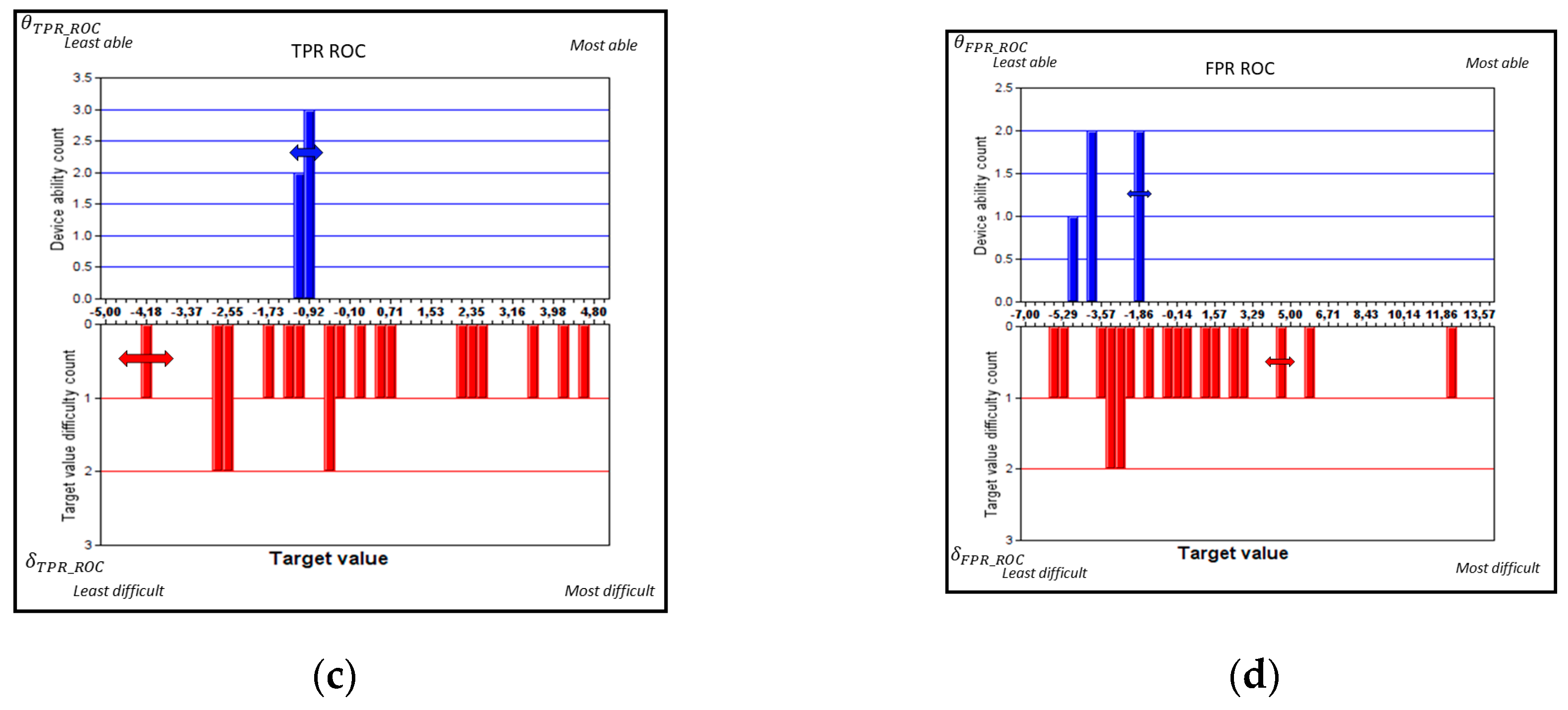
, of each assigned value (task), j, on a common interval scale. Figure 3 show the results of the logistic regression for the two tested ways of applying the Rasch model (Section 3.4.2, i.e., calculated (i) the classic for each target value for each decision scenario (positives and negatives); and (ii) from the cumulative rates for TPR and FPR (Figure A1)).
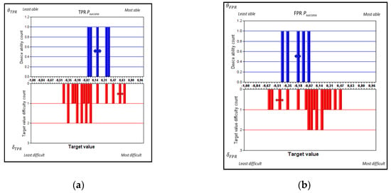
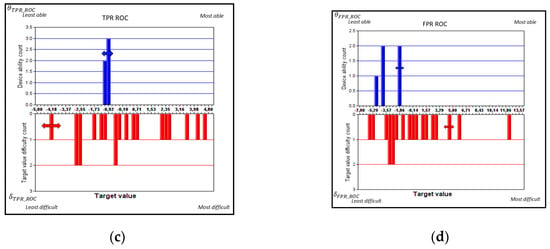
Figure 3.
Histograms of experimental data with Rasch estimates of device ability (, upper histograms) and target value difficulty ( lower histograms) based on for (a) scoring alternative (i) for negatives and (b) scoring alternative (ii) FPR, as well as (c) scoring alternative (i) for positives and (d) scoring alternative (ii) TPR for five device types used for pregnancy testing. Measurement uncertainty coverage factors k = 2. (The height of each column in these histograms—called “Count”—indicates, as standard, the occupancy of each probability mass function; that is, the number of device types (upper, blue plots) and target level tasks (lower, red plots) per bin, respectively.
From an inspection of the Rasch histograms of Figure 3, it seems that device–task targeting is better when alternative (i), i.e., classic , Figure 3a,b, is used; that is, there is better matching in terms of spread and centring between the spans of ability and difficulty. Better targeting according to the Rasch approach [18] leads to lower measurement uncertainties for device abilities and a better separation between the devices with method (i). On the other hand, measurement uncertainties for target values are larger when alternative (i) (i.e., classic ) was used, except for the highest and lowest target values where the cumulative rates were almost 100% or 0%. Method (i) is better in terms of separating the devices, as will be examined in detail in Section 4.5. For the corresponding (ii) ROC-based values, Figure 3c,d, the resolution of the device ability is poorer.
Depending on how scoring is carried out, the order of item difficulty will change, as the orderings depend on how one values a high probability for the various decision risks (see Section 4.2).
4.2. Rasch Parameters Versus Assigned Value, x
Using the property of specific objectivity offered by the Rasch model (Appendix A.2) allows the variation in task difficulty to be examined (Figure 4), irrespective of which of the five device types are being used.


Figure 4.
Rasch estimates of target value difficulty () based on for (a) scoring alternative (i) for positives; (b) scoring alternative (i) for negatives; (c) scoring alternative (ii) for positives and (d) scoring alternative (ii) for negatives for a combination of all five device types used for pregnancy testing. Measurement uncertainty coverage factors k = 2.
These observed trends can be compared with the predictions of our adopted model of the level of difficulty for correct classification, inspired by the work of Bashkansky and Turetsky [19] regarding the ‘difficulty of detecting a shift with a control chart’, citing Montgomery [20], as explained in Section 3.4.2 and Appendix A.3.
As shown in Figure 4a,c, for TPR, the general trends in δ versus x is, as expected, that task difficulty is highest at the lowest target concentrations and decreases linearly with x, reaching a minimum difficulty at SL (where task difficulty , i.e., and ). The theory of Bashkansky and Turetsky [19], Appendix A.3 makes no prediction regarding how task difficulty trends beyond the specification limit, SL). Apart from a rescaling, the same trend in δ versus x is found for both scoring alternatives.
The trend is the opposite for FPR (Figure 4b,d), where task difficulty is least at the lowest target concentrations and increases linearly with x, reaching a maximum difficulty at SL (where task difficulty ). Otherwise, the same trend in δ versus x is found for both scoring alternatives, as found also for TPR. An explanation of the opposite trends of TPR and FPR task difficulty versus concentration has to do with how, for each kind of decision risk, a “successful” classification is rated; arguably, a higher probability of false positive classification (“fall-out”) should be valued negatively, in contrast to the positive rating of successful true positive classification (“specificity”).
What is more, we can make estimates regarding the specification limit from the intercept () on the x-axis of each plot shown in Figure 4 by making linear regressions of Equation (2) over the range up to where the line crosses the x-axis, with the following results:
and
where m and c are, respectively, the slope and intercept (on the y-axis) of each straight line fitted to the data of δ versus x up to SL in accord with the theory (Appendix A.3). These estimates are reasonably close to the expected diagnostic value, such as 25 hCG (IU/L).
4.3. Evaluating Device Parameters
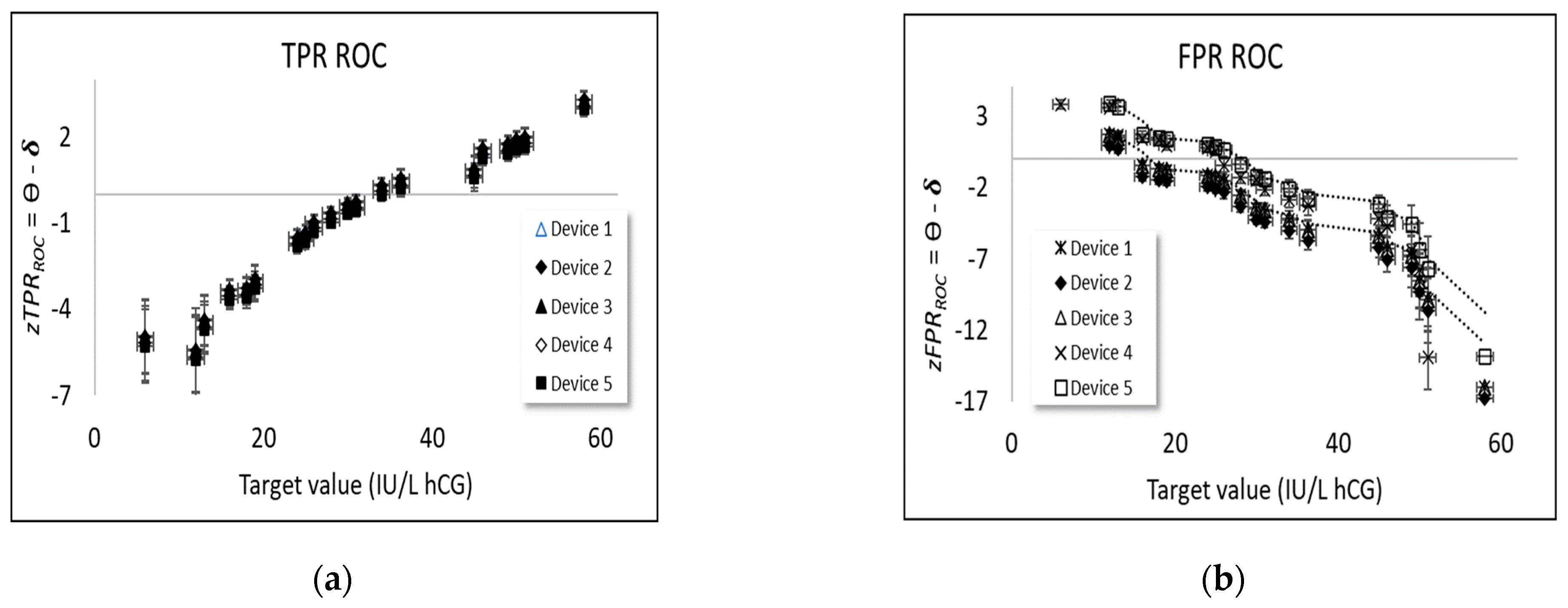
In order to evaluate the slope, M, and intercept, C, of the new kind of plots for the different device types (Section 3.4.2), estimates of u and SL for each device were obtained by linear regression of the plots in Figure 5 for each coordinate and , respectively, versus the target value, , according to the theoretical model (Equation (A2)). From the separate Rasch estimates of task difficulty and device ability, thanks to the principle of specific objectivity (Appendix A.2), it is straightforward to calculate
and for curves versus assigned value, x, Hcg (IU/L) for the five devices used for pregnancy testing, based on the two methods (Section 4.1), respectively.
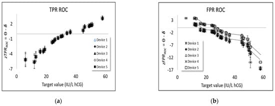
Figure 5.
Experimental studies of Rasch parameters based on for scoring alternative (ii) for (a) positives and (b) negatives versus assigned value, hCG (IU/L) for five device types used for pregnancy testing. Measurement uncertainty coverage factors k = 2.
The plots (Figure 5) for each coordinate and , respectively, versus the target value, , show sets of parallel lines where the common slope of each set of lines corresponds to the (inverse) classification uncertainty, u, of the set of items from the principle of specific objectivity (Appendix A.2). The set of parallel lines for FPR are better resolved for the two methods, aligning with the Rasch histogram plots (Figure 3) which show more distinct device ability variation for the false positive rates. In fact, most of the differences between the curves in Figure 5 (particularly pronounced in Figure 5b) are due to the differences in Rasch abilities and among the different device types as estimated with a Rasch logistic regression as described in Section 4.1. (The closeness of the curves, particularly in Figure 5a, indeed makes it difficult to distinguish the symbols denoting them; this is a result, not a shortcoming in figure quality.)
In contrast to the fitting procedure (Section 4.2) used over the range 6 < x < SL (IU/L) in Figure 4, for the plots, an approximate linear relation is assumed across the whole range of target concentration values 6 < x < 60 (IU/L) in order to match the range adopted when plotting traditional ROC curves (Appendix A.1). Note that this procedure extrapolates the theory of Bashkansky and Turetsky [19] (Appendix A.3) beyond the specification limit, SL.
As an example, an analysis of the FPR plot (Figure 5b) yielded the following values for device 1:
and
(The negative sign on the uncertainty has to do with the opposite slope of FPR rating, as discussed in Section 3.2).
The parameter estimates obtained by these linear regressions across the whole range of target concentration values 6 < x < 60 (IU/L) (to match the range adopted when plotting traditional ROC curves) are given in Table 3. Uncertainties, quoted in parentheses, have coverage factors k = 2. It can be noted that the SL estimates with these linear regressions over the whole concentration range deviate more from the corresponding SL estimate (of 25 IU/L) than with the method described in Section 4.2. A principal reason for these discrepancies is that the theory of Bashkansky and Turetsky ([19], Appendix A.3) does not strictly apply for concentrations around SL where the probability of successful classification asymptotically approaches 100%.

Table 3.
Summary of device type parameters.
4.4. Theoretical Curves
The theoretical values of the slope, C, and intercept, M, of the new plots for each device (Section 3.4.2) can now be estimated using the u and SL values for each device obtained by linear regression of each coordinate and , respectively, versus the target value, (Figure 5b–d). For example, for device 1:
and
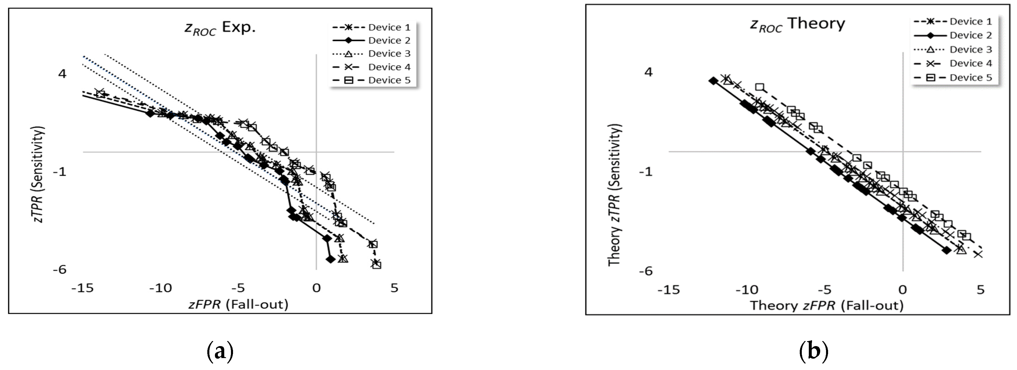
Table 4 shows a satisfactory agreement between C and M for the theoretical and experimental curves (Pearson correlation coefficients 0.91) for all device types, respectively, as also shown in corresponding plots (Figure 6a,b).

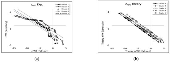
Figure 6.
curves for the five devices used for pregnancy testing (a) experiment (uncertainty coverage factors, k = 2) and (b) theory. (The dotted lines indicate linear regressions to each curve, as expressed by the equations y versus x).
4.5. Assessing Relative Performance of Devices
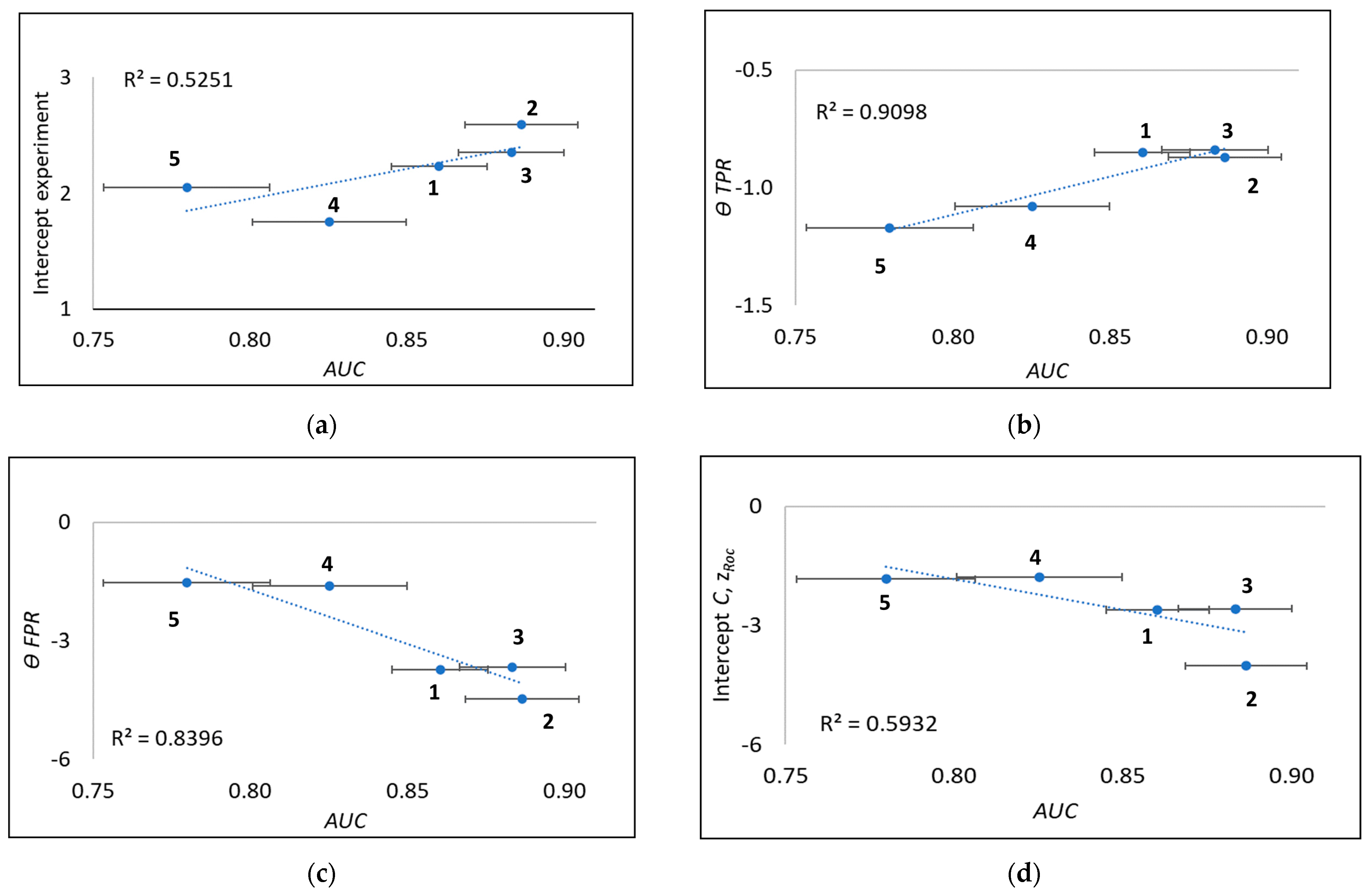
Linacre [12] proposed using the intercept, c, of each of his linearised ROC curves (Section 3.4.1 and Figure 2) as a better measure of device performance than the traditional AUC (Appendix A.1). A comparison between Linacre c intercepts and AUC for the five device types studied here for pregnancy testing is shown in Figure 7a (Pearson correlation coefficient R = 0.73).
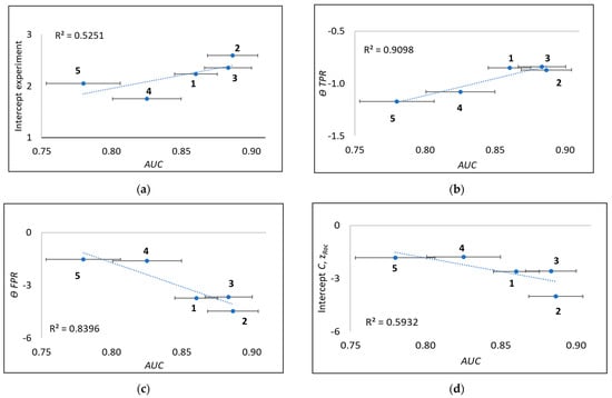
Figure 7.
AUC values compared to (a) experimental Linacre c intercepts, (b) device ability , (c) device ability , and (d) new zROC plot intercepts C for the five device types (1,…,5) used for pregnancy testing.
In this work, we additionally first assessed the correlation between the Rasch device abilities and vs. AUC (Section 3.4.2). Figure 7b,c shows that those correlation coefficients (0.95 and 0.92) are comparable with each other and that both are better than Linacre’s plots (Figure 7a). The degree of correlation between and is found to be 0.94 (as expected, the average of the correlations shown in Figure 7b,c) Finally, the new zROC plot intercepts C (Figure 7d) and correlates slightly better (0.77) than Linacre’s (Figure 7a) but less well than the other alternatives based on the Rasch parameters, and . This poorer performance of the linearisation plots reflects limitations in extending linear regression over the full concentration span to match traditional ROC practice (Section 4.3), rather than only up to SL, in accordance with the theory (Appendix A.3).
In summary, the new linearised ROC curves adopting the Rasch model are better correlated with AUC than the Linacre [12] approach of using the intercepts, but both linearisation methods (with the results shown in Figure 7a,d, respectively) perform less well than our new Rasch ability method (results shown in Figure 7b,c). This new method—evaluating device ability in terms of and from separate Rasch regressions for each axis of ROC curves—performs significantly better and is therefore recommended to replace traditional methods of evaluating device ability.
4.6. Measurement Uncertainties
Logistic regressions (Section 4.1) with the Rasch formula (Equation (1)) also furnish estimates of the expanded (Coverage factor, k = 2) measurement uncertainties (details of how these uncertainties are derived can be found in any Rasch program documentation, such as the WINSTEPS® manual), in the abilities, , of each device type (Table 3) and , in the level of difficulty, , of each task. Those measurement uncertainties can be used to add uncertainty intervals to traditional ROC curves (example shown for device type 1 in Figure 8) by calculating for each device type an upper and lower curve where the combined, expanded uncertainty:
is, respectively, added or subtracted to each logistic curve:
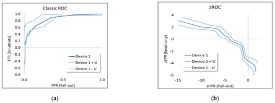
Figure 8.
ROC curves with uncertainty intervals (uncertainty coverage factors, k = 2) for device type 1 used for pregnancy testing with (a) classic ROC and (b) .
Figure 8.
ROC curves with uncertainty intervals (uncertainty coverage factors, k = 2) for device type 1 used for pregnancy testing with (a) classic ROC and (b) .
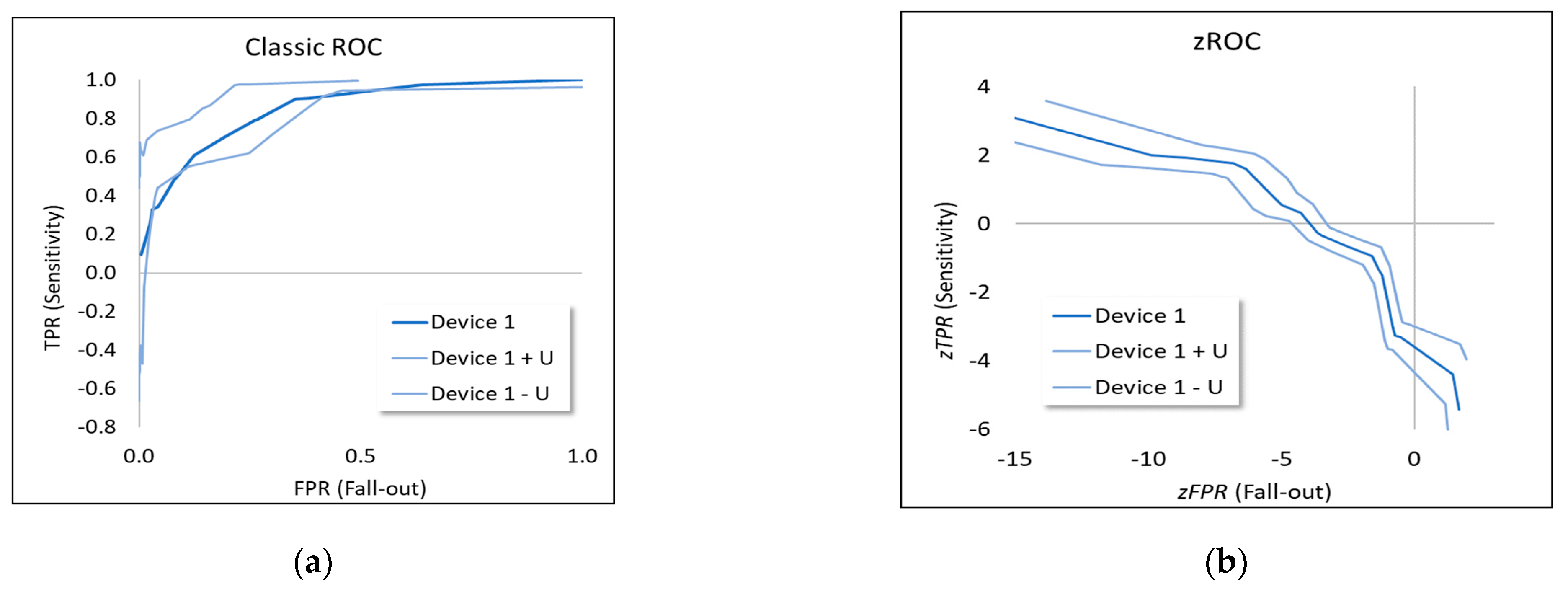
Comparing the scatter between the upper and lower ROC curves (shown in traditional form for device type 1 in Figure 8a) with the measurement uncertainties for the different device types shown in Table 3 gives an indication of how reliably one can distinguish true differences in device type performance from apparent scatter due to uncertainty and limited measurement quality. As pointed out above, such comparisons are particularly challenging for traditional ROC curves (Figure 1) since not only are ROC curves more difficult technically to interpret than straight lines [12], but they are also affected by counted fraction ordinality (Appendix A.1).
In Figure 8b, a corresponding plot with measurement uncertainties for the curves based on the cumulative rates (Figure 5a) is shown for device type 1. When comparing Figure 8a,b, measurement uncertainties are suppressed in Figure 8a at either extreme of the scale when not compensating for counted fraction ordinality while, as shown more clearly in Figure 8b, measurement uncertainties at the upper and lower end of the scale actually increase due to less information at the scale extremes regarding the performance, leading, in turn, to less accuracy in determining device type ability. Secondly, the response probabilities of traditional ROC curves in general confound the level of difficulty of the classification task with the ability of the classifier to make a correct classification. The latter point—concerning what Rasch referred to as specific objectivity—is examined in detail in the next and final part of the Results section.
4.7. Limitations
In assessing potential limitations in the present study, known limitations in both approaches can be noted.
Rasch logistic regression depends on the assumption that a single dimension underlies the explanatory variable determining classification task difficulty and there are standard tests for establishing the unidimensionality, such as an examination of clustering in principal component analyses (PCA), of the residuals of Rasch logistic regressions. It is conceivable that task difficulty at the highest hCG concentration levels belongs to a different dimension than that of determining classification difficulty at low concentrations, which warrants further investigation.
In this work, we have tested two approaches (Section 3.4.2) to Rasch logistic regression of ROC curves where the probability of successful classification, , is calculated (i) for each device and concentration level individually and (ii) at each concentration level, estimating the cumulative rates for TPR and TNR. These alternative calculations yielded different estimates of device ability, as plotted in Figure 3.
The preliminary PCA results indicate for all four modes of calculation only small (less than 1%) unexplained variances. So-called construct alleys are another tool to assess the assumptions—such as scale sensitivity—behind regular Rasch logistic regressions [8].
Such effects may influence both calculations (Section 3.4.2) according to method (i)—that is, conventional Rasch regression—but arguably perhaps even more in method (ii), since the sums included in the ROC expressions for TPR and TNR cover not only scores for the device at the target value of interest, but also for all other target values.
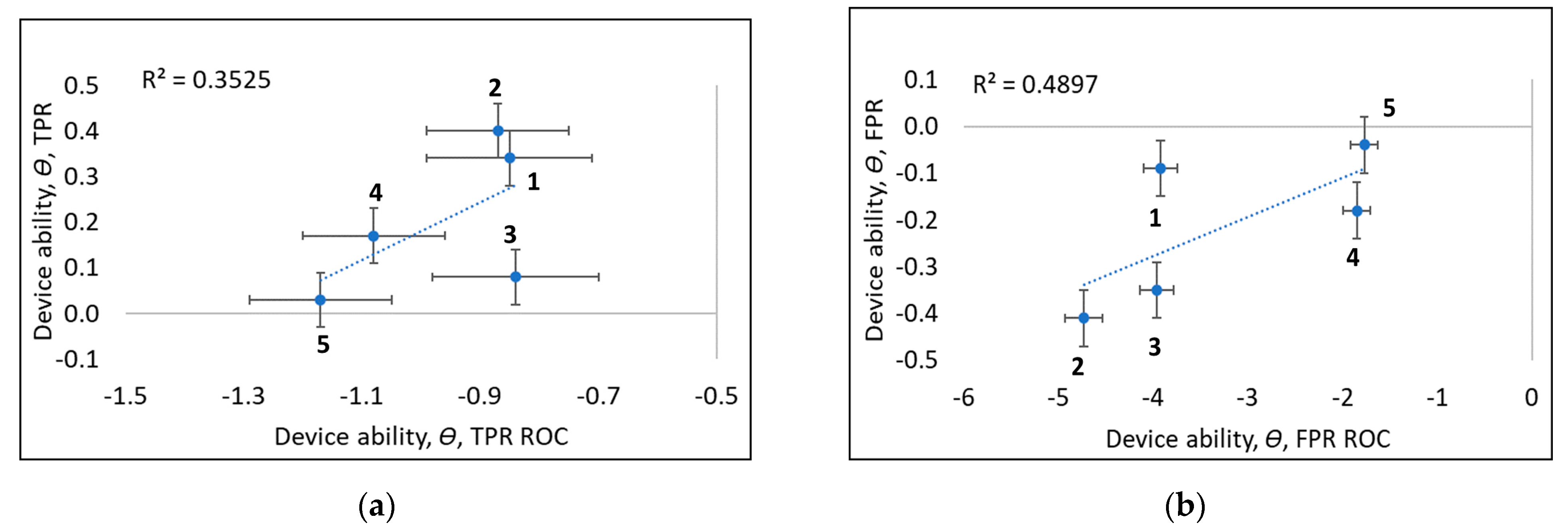
Potential limitations in the two methods of calculation, such as the multidimensionality in task difficulty estimation, could also influence estimates of device ability since the Rasch model (Equation (1)) solves for difficulty and ability conjointly. Such effects, which would indicate a breakdown in specific objectivity (Appendix A.2), might be revealed by inspecting plots of device ability with the two alternative methods, as shown in Figure 9. In Figure 9a, for TPR, the device abilities with a cumulative Rasch-based analysis (x-axis) are unable to resolve individual device abilities, while conventional Rasch methodology (y-axis) shows clear differences in ability between the two groups of devices. (Higher logit values correspond to higher device ability). In Figure 9b, for TNR, a corresponding separation of the two groups of devices is shown while there are fewer measurement uncertainties for the cumulative Rasch-based analysis. Interestingly, there are clearly two devices (no. 4 and 5) performing much better with the cumulative Rasch-based analysis of TNR (x-axis of Figure 9b) compared with a conventional Rasch methodology (y-axis of Figure 9b). This could be explained by this device having fewer data compared to the other devices (Table 1), both in terms of tested target values and the number of tests per target values.
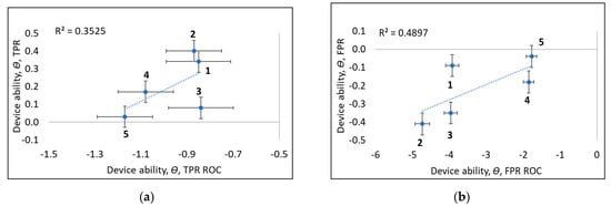
Figure 9.
Experimental studies of device ability, ϴ, (a) TPR and (b) TNR for the two estimates (i) y-axis and (ii) x-axis for five device types (1,…, 5) used for pregnancy testing.
Bashkansky and Turetsky [19] have emphasised that two parameters are key to explaining task difficulty: (i) the estimate of SL and (ii) the classification uncertainty, u. As already presented, the fitting procedure (Section 4.2) used for task difficulty over the range 6 < x < SL (IU/L) in Figure 4 yields estimates of SL close to the diagnostic value. However, in contrast, the new plots (Section 4.4) (as well as Linacre’s plots) reveal only approximate linear relations, with estimated SL further from the diagnostic value, when spanning the whole range of target concentration values 6 < x < 60 (IU/L), that is, beyond the specification limit, SL, to match the range adopted when plotting traditional ROC curves. These poorer fits may explain why ROC curves are less successful at resolving differences in device type ability (Figure 7a,d) compared with our new method (Figure 7b,c). In other words, ROC curves attempt to cover too many effects at once.
5. Conclusions
In this paper, we have argued for and demonstrated the added value of a modernisation of the traditional ROC curve methodology, bringing it up to date with modern measurement theory. Inherent and often unacknowledged challenges implicit to the ROC tool as part of CTT, such as non-linearity, effects of ordinality, and confounding task difficulty and instrument ability, are met here with a novel approach combining measurement system analysis and item response theory (IRT), using data from pregnancy testing as an example.
This methodology should be competitive with other alternatives, such as rankits (Appendix A), and also goes some way to meeting earlier criticism that separate information about TPR (sensitivity) and FPR (1—specificity, fall-out) was lost, and that no distinctions were made for differences in device-specific SL when plotting traditional ROC curves [10].
We have re-examined and built on earlier studies of ROC curves for the assessment of device type classification performance using an approach combining MSA and IRT. The proposed modernised ROC goes some way to meeting the challenges posed by Linacre [12] in his original criticism of traditional ROC curves, including handling the non-linear % metrics TPR and FPR. The values of device ability from separate Rasch IRT regressions for each axis of ROC curves were found to perform significantly better and are recommended to replace other approaches for device assessment, with correlation coefficients with traditional area-under-curve metrics of at least 0.92, which exceeded that of linearised ROC plots, such as Linacre’s (Section 4.5). Measurement uncertainties in ROC curves were evaluated (Section 4.6), which also constitute an important part of assuring the measurement quality of each ROC curve.
The limitations in the present study have been identified (Section 4.7). Future studies remain to be made and will be applied to other sets of data, including an extension of the univariate studies presented here to include multivariate decision risks and more complete data sets. We also recommend further investigations of the appropriateness of using a cumulative Rasch-based analysis in order to not diminish full specific objectivity (Appendix A.2).
The new methodology should enable more reliable decision-making in conformity assessment in the presence of measurement uncertainty applicable to many decision-making scenarios, ranging from pregnancy testing (as studied here) to machine learning, where use of the ROC curve as a metric for assessing machine learning algorithms has become almost indispensable [9].
Author Contributions
Conceptualisation, L.R.P. and J.M.; methodology, L.R.P.; validation, J.M., A.S. and G.N.; formal analysis, L.R.P.; data curation, A.S. and G.N.; writing—original draft preparation, L.R.P.; writing—review and editing, J.M., A.S. and G.N.; visualisation, J.M. All authors have read and agreed to the published version of the manuscript.
Funding
Part of the work reported has also been part of the 15HLT04 NeuroMET and 18HLT09 NeuroMET2 projects which received funding (2016–2022) from the EMPIR programme co-financed by the Participating States and from the European Union’s Horizon 2020 research and innovation programme. Hence, we would like to express our great appreciation to collaborators and partners for our valuable and constructive work together.
Data Availability Statement
hCG data from proficiency testing has been kindly provided by: Equalis Uppsala (SE) and Noklus Bergen (NO).
Acknowledgments
This work is based on learnings and outcomes in several projects during the past years, including the RISE internal platform for category-based measurements.
Conflicts of Interest
The authors declare no conflict of interest.
Appendix A. ROC, Item Response Theory, Control Charts, Rankits and Other Measures
Appendix A.1. ROC in the Presence of Counted-Fractions Ordinality
A generic version of a ROC plot is given by Birdsall [11] for the case of a binary decision or about an entity subject to conformity assessment based on a signal ( with noise) in the presence of noise, , where the vertical axes of the plot can be either the probability or while the horizontal axes can be either or . This description has wide applicability, including for both pregnancy testing (as in the present case study) as well as in assessing the performance of machine learning classification algorithms [9].
These probabilities can be calculated from the raw testing data (exemplified in Table 1, with expressions such as those given in the following “decision matrix” (1)) (Figure A1).
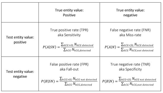
Figure A1.
Decision matrix.
Figure A1.
Decision matrix.

A traditional ROC curve is produced by calculating the probabilities and at each assigned value (hCG (IU/L) in the present case study) to yield estimates of TPR and FPR, respectively. In making the summations, each local SL is allowed to “sweep successively over” the complete range of concentration levels for each device type from the actual concentration level and upwards [11]. ROC curves for each device are then plotted with TPR against FPR, shown for the present case study in Figure 1.
A poorly performing instrument would have a ROC curve as a 45° straight line between the coordinates (0,0) and (1,1). AUC (area under curve) values are traditionally used to estimate relative classification performance, calculated as in [21]:
or in [22]:
Other diagnostic accuracy indices regularly used in ROC analysis include:
- The Youden index, which is a measure of the vertical distance between the 45° line (Section 3.1) and the corresponding point on the ROC curve, as given by the expression . A better diagnosis has a higher Youden index value [23]
- Sensitivity + Specificity, which is a simple addition where a better diagnosis has a higher index value.
- Distance to corner, a better diagnosis which has a smaller distance, d, to the top-left corner of the ROC curve for each cut-off value,
All of these and similar traditional ROC performance indices unfortunately do not take account of the effects of uncompensated ordinality, particularly the well-known non-linearity of data scaling due to the effects of so-called ‘counted fractions’; put simply, any score on a fixed scale bounded by 0 and 100% becomes increasingly non-linear at either extreme [5]. A difference of, for example, 1% percentage points in score X is a different amount at mid-scale (50%) compared with scores at 5% or 95%. Classic test theory (CTT) does not compensate for ‘counted fractions’ ordinality of percentage raw scores nor makes a separation of classifier ability from task difficulty which are confounded in the raw data, as described in Appendix A.2.
Merely using a non-parametric test, such as Kruskal–Wallis or other ranking tests, to deal with any ordinality instead of adopting modern measurement theory can make it challenging to detect significant correlations, for instance those between cognitive scores and biomarkers, or in assessing classification performance as studied here with ROCs. The under-estimation due to counted fractions at the high end of a cognitive scale [24], for instance, can easily be misinterpreted in terms of other effects, such as ‘cognitive reserve’. Rankits are considered further in Appendix A.3.
Appropriate approaches—as presented below—to compensating for the effects of scale non-linearity and unrecognised ordinality have been known a long time but are apparently often ignored, and uptake of modern approaches has been slow.
Appendix A.2. Rasch, MSA and Specific Objectivity
A key development in modern measurement theory is the psychometric approach of Rasch [18]. A special feature of the Rasch approach [18] is being able to, with Equation (1), make separate estimates for classifier ability and classification task difficulty, which are confounded in the raw data according to Rasch’s principle of specific objectivity.
The Rasch model, developed about twenty years after the first ROC curves, adopted a radically different approach to statistical evaluation, as summarised in Rasch’s [18] words:
‘Zubin et al. (1959) expresses: “Recourse must be had to individual statistics, treating each patient as a separate universe. Unfortunately, present day statistical methods are entirely group-centered so that there is a real need for developing individual-centered statistics.”’
‘Individual-centered statistical techniques require models in which each individual is characterised separately and from which, given adequate data, the individual parameters can be estimated…. Symmetrically, it ought to be possible to compare stimuli belonging to the same class—“measuring the same thing”—independent of which particular individuals within a class considered were instrumental for the comparison.’
This separation is key in metrology, and is particularly important to consider when assuring metrological quality of performance tests and other classification data.
Although Rasch [25] did not use the MSA approach and terminology (described in Section 3.2), an early form of his psychometric model, in response to the contemporary demands for individual measures, was very much an MSA formulation [4]. He posited that the odds ratio of successfully performing a task is equal to the ratio of an ability, h, (Rasch [18] used the person attribute ’inability’ instead, given by ), to a difficulty, k:
where the test person (“agent”) ability, , and task (“object”) difficulty, (or other item:probe pairs of attributes).
The probability of a ‘correct’ response on item j by a rater i is cumulative, and the cumulative distribution function of the logistic distribution for the Rasch model is an operating characteristic function (OCF) [26]. The Rasch approach essentially compensates for the ‘counted fractions’ ordinality (Appendix A.1).
The original Rasch [25] formulation referred to a probabilistic Poisson distribution:
This distribution is well known from quality control as a model of the number of defects or nonconformities that occur in a unit of product when classifying it, where x is the quality characteristic being classified [20]. The parameter is equal directly both to the mean and variance of the Poisson distribution. In Rasch’s [25] model:
where h and k are defined in Equation (A1).
Appendix A.3. Ability and Task Difficulty in Control Charts
Explanations that outline how classification task difficulty and classifier ability vary with a quality characteristic can be sought in earlier theories of control charts from statistical quality control, as noted by Bashkansky and Turetsky [19]. Montgomery [20] considered the ‘ability of detecting a shift in mean with a control chart’ for an explanatory variable, x, measured n times, with a normally distributed mean:
Here, the mean of the control chart is shifted:
compared with the control limit which lies at a distance, , from :
The risk, arising from of a false positive decision (FP, ‘fall out’), for instance, is equal to the cumulative probability above while is within specification:
In the modern terminology of the Rasch formula of Equation (1), the decision risk, will depend, according to Bashkansky and Turetsky [19], on both (“agent”) ability, , and (“object”) difficulty, in units of . In turn, this gives:
and leads to:
This is the basic expression, with the substitutions , used in Equation (2) to quantify how classification task difficulty and classifier ability vary with a quality characteristic in the present study.
The rankit approach has been employed in case studies similar to the present study [7]. In that approach, the observed values are ordered in terms of their relative magnitudes as ranks, which can be compared with the Rasch approach to compensating for ordinality as follows:
However, ranking data instead of compensating for known counted fractions effects (Appendix A.1) means that valuable, quantitative information is lost. It is unclear how measurement uncertainty, such as might increase by uncorrected nonlinearity, will affect the ranking of raw scores in non-parametric tests. As noted in A1, there seems to be little sense in attempting to correlate merely ranked data with fully quantitative instrument data for other physical properties.
Appendix B. Explaining Curve Parameters
From Equation (2), variation of (classification difficulty) with on either axis (TPR or FPR) of a curve, would yield a straight line against the marker value, , with slope , according to A3. As exemplified in Figure 4, in the present case the slopes of these straight lines change little, meaning that the classification uncertainty, u, is largely the same for the different device types.
There are two intercepts of interest which characterise the straight line of z against x for each axis of the curve separately (Figure 4):
- The straight line intercepts the vertical axis, where x = 0 (and ), at a place which shifts with the ability, , of each device;
- The straight line crosses the horizontal (x-) axis at z = 0, where and . The different values of SL obtained in this fashion match the different intercepts on the vertical axis, that are due to the varying device ability.
The overall curve would thereafter be a line with slope and intercept according to the equation: of a plot, expressed in terms of the various parameters occurring in the formulae for the straight lines associated with each axis (Figure 5):
and
References
- Pendrill, L.R. Using Measurement Uncertainty in Decision-Making and Conformity Assessment. Metrologia 2014, 51, S206–S218. [Google Scholar] [CrossRef]
- Hibbert, D.B. Evaluation of Measurement Data: The Role of Measurement Uncertainty in Conformity Assessment. Chem. Int.—Newsmag. IUPAC 2013, 35, 22–23. [Google Scholar] [CrossRef]
- Peterson, W.; Birdsall, T.; Fox, W. The Theory of Signal Detectability. Trans. IRE Prof. Group Inf. Theory 1954, 4, 171–212. [Google Scholar] [CrossRef]
- Pendrill, L. Quality Assured Measurement: Unification across Social and Physical Sciences; Springer Series in Measurement Science and Technology; Springer International Publishing: Berlin/Heidelberg, Germany, 2019; ISBN 978-3-030-28694-1. [Google Scholar]
- Mosteller, F.; Tukey, J. Data Analysis and Regression: A Second Course in Statistics, 1st ed.; Pearson: Reading, MA, USA, 1977; ISBN 978-0-201-04854-4. [Google Scholar]
- Koczula, K.M.; Gallotta, A. Lateral Flow Assays. Essays Biochem. 2016, 60, 111–120. [Google Scholar] [CrossRef] [PubMed]
- Petersen, P.H.; Christensen, N.G.; Sandberg, S.; Nordin, G.; Pedersen, M. How to Deal with Semi-Quantitative Tests? Application of an Ordinal Scale Model to Measurements of Urine Glucose. Scand. J. Clin. Lab. Investig. 2009, 69, 662–672. [Google Scholar] [CrossRef] [PubMed]
- Somborac Bačura, A.; Dorotić, M.; Grošić, L.; Džimbeg, M.; Dodig, S. Current Status of the Lateral Flow Immunoassay for the Detection of SARS-CoV-2 in Nasopharyngeal Swabs. Biochem. Med. 2021, 31, 020601. [Google Scholar] [CrossRef] [PubMed]
- Majnik, M.; Bosnić, Z. ROC Analysis of Classifiers in Machine Learning: A Survey. Intell. Data Anal. 2013, 17, 531–558. [Google Scholar] [CrossRef]
- Krouwer, J.S. Cumulative Distribution Analysis Graphs—An Alternative to ROC Curves. Clin. Chem. 1987, 33, 2305–2306. [Google Scholar] [CrossRef] [PubMed]
- Birdsall, T. The Theory of Signal Detectability: ROC Curves and Their Character; University of Michigan Library: Ann Arbor, MI, USA, 1973. [Google Scholar]
- Linacre, J. Evaluating a Screening Test. Rasch Meas. Trans. 1994, 7, 317–318. [Google Scholar]
- Cipriani, D.; Fox, C.; Khuder, S.; Boudreau, N. Comparing Rasch Analyses Probability Estimates to Sensitivity, Specificity and Likelihood Ratios When Examining the Utility of Medical Diagnostic Tests. J. Appl. Meas. 2005, 6, 180–201. [Google Scholar] [PubMed]
- Fisher, W.P., Jr.; Burton, E. Embedding Measurement within Existing Computerized Data Systems: Scaling Clinical Laboratory and Medical Records Heart Failure Data to Predict ICU Admission. J. Appl. Meas. 2010, 11, 271–287. [Google Scholar] [PubMed]
- Wright, B.D.; Perkins, K.; Dorsey, K. Multiple Regression via Measurement. Rasch Meas. Trans. 2000, 14, 729. [Google Scholar]
- Schlattmann, P. Tutorial: Statistical Methods for the Meta-Analysis of Diagnostic Test Accuracy Studies. Clin. Chem. Lab. Med. 2023, 61, 777–794. [Google Scholar] [CrossRef] [PubMed]
- E11 Committee. Guide for Measurement Systems Analysis (MSA); ASTM International: West Conshohocken, PA, USA, 2022. [Google Scholar]
- Rasch, G. Studies in Mathematical Psychology: I. Probabilistic Models for Some Intelligence and Attainment Tests; Nielsen & Lydiche: Oxford, UK, 1960. [Google Scholar]
- Bashkansky, E.; Turetsky, V. Ability Evaluation by Binary Tests: Problems, Challenges & Recent Advances. J. Phys. Conf. Ser. 2016, 772, 012012. [Google Scholar] [CrossRef]
- Montgomery, D.C. Introduction to Statistical Quality Control, 3rd ed.; Wiley: New York, NY, USA, 1996; ISBN 978-0-471-30353-4. [Google Scholar]
- Statology. Zach How to Create a ROC Curve in Excel (Step-by-Step). 2021. Available online: https://www.statology.org/roc-curve-excel/ (accessed on 10 May 2023).
- Safari, S.; Baratloo, A.; Elfil, M.; Negida, A. Evidence Based Emergency Medicine; Part 5 Receiver Operating Characteristic Curve and Area under the Curve. Emergency 2016, 4, 111. [Google Scholar] [PubMed]
- Youden, W.J. Index for Rating Diagnostic Tests. Cancer 1950, 3, 32–35. [Google Scholar] [CrossRef] [PubMed]
- Pendrill, L.R.; Melin, J. Assuring Measurement Quality in Person-Centered Care. In Person-Centered Outcome Metrology: Principles and Applications for High Stakes Decision Making; Fisher, W.P., Jr., William, P., Cano, S.J., Eds.; Springer Series in Measurement Science and Technology; Springer International Publishing: Cham, Switzerland, 2023; pp. 311–355. ISBN 978-3-031-07465-3. [Google Scholar]
- Rasch, G. On General Laws and the Meaning of Measurement. In Psychology, Proceedings of the Fourth Berkeley Symposium on Mathematical Statistics and Probability, Volume 4: Contributions to Biology and Problems of Medicine, Berkeley, CA, USA, 20 June–30 July 1960; University of California Press: Oakland, CA, USA, 1961; pp. 321–333. [Google Scholar]
- Wind, S.A. Examining Rating Scales Using Rasch and Mokken Models for Rater-Mediated Assessments. J. Appl. Meas. 2014, 15, 100–132. [Google Scholar] [PubMed]
Disclaimer/Publisher’s Note: The statements, opinions and data contained in all publications are solely those of the individual author(s) and contributor(s) and not of MDPI and/or the editor(s). MDPI and/or the editor(s) disclaim responsibility for any injury to people or property resulting from any ideas, methods, instructions or products referred to in the content. |
© 2023 by the authors. Licensee MDPI, Basel, Switzerland. This article is an open access article distributed under the terms and conditions of the Creative Commons Attribution (CC BY) license (https://creativecommons.org/licenses/by/4.0/).

