Method for Determining the Dominant Type of Human Breathing Using Motion Capture and Machine Learning

Abstract

Since the COVID-19 pandemic, the demand for respiratory rehabilitation has significantly increased. This makes developing home (remote) rehabilitation methods using modern technology essential. New techniques and tools, including wireless sensors and motion capture systems, have been developed to implement remote respiratory rehabilitation. Significant attention during respiratory rehabilitation is paid to the type of human breathing. Remote rehabilitation requires the development of automated methods of breath analysis. Most currently developed methods for analyzing breathing do not work with different types of breathing. These methods are either designed for one type (for example, diaphragmatic) or simply analyze the lungs’ condition. Developing methods of determining the types of human breathing is necessary for conducting remote respiratory rehabilitation efficiently. We propose a method of determining the type of breathing using wireless sensors with the motion capture system. To develop that method, spectral analysis and machine learning methods were used to detect the prevailing spectrum, the marker coordinates, and the prevailing frequency for different types of breathing. An algorithm for determining the type of human breathing is described. It is based on approximating the shape of graphs of distances between markers using sinusoidal waves. Based on the features of the resulting waves, we trained machine learning models to determine the types of breathing. After the first stage of training, we found that the maximum accuracy of machine learning models was below 0.63, which was too low to be reliably used in respiratory rehabilitation. Based on the analysis of the obtained accuracy, the training and running time of the models, and the error function, we choose the strategy of achieving higher accuracy by increasing the training and running time of the model and using a two-stage method, composed of two machine learning models, trained separately. The first model determines whether the breath is of the mixed type; if it does not predict the mixed type of breathing, the second model determines whether breathing is thoracic or abdominal. The highest accuracy achieved by the composite model was 0.81, which surpasses single models and is high enough for use in respiratory rehabilitation. Therefore, using three wireless sensors placed on the patient’s body and a two-stage algorithm using machine learning models, it was possible to determine the type of human breathing with high enough precision to conduct remote respiratory rehabilitation. The developed algorithm can be used in building rehabilitation applications.

1. Introduction

The COVID-19 epidemic provoked a large amount of research, not only on the virus itself but also on the effects of the virus on humans. One of the essential kinds of rehabilitation after COVID-19 is respiratory rehabilitation. It helps to develop the intercostal muscles and diaphragm to increase respiratory potential. This increase in respiratory potential occurs when the patient has a mixed type of breathing, which can be obtained by repeating a set of special exercises during the rehabilitation process. If the patient has the wrong type of breathing, they can be given instructions to correct it, so determining the exact type of breathing is a relevant problem in modern rehabilitology. According to the interviewed rehabilitologists, as part of the training, it is necessary to correctly determine at least 3/4 respiratory cycles.

The rehabilitation process is very labor-intensive, but it can be automatized using gaming practices, for example, by introducing score points, which makes it more accessible and attractive. This will help to lower the workload of doctors and rehabilitologists [1,2].

The importance of breathing and its impact on the state of the human body is widely recognized by modern doctors and scientists [3,4], so the target user group for respiratory rehabilitation is not limited to post-COVID-19 patients.

In modern information technology, wireless sensors, wireless sensor networks (WSN), motion capture systems, crowdsensing, virtual reality technologies, etc. are often used to improve productivity, efficiency, and security [5,6,7] when solving various problems in different areas: e.g., in ecology [7], the early detection of fires and landslides became possible with the help of WSNs; they also help monitor air quality. In military applications, WSNs track the enemy actions and help make decisions about the further movement of armed forces [8]. Medicine is no exception. Sensors and WSNs are used to improve patient care in rehabilitation and diagnostic processes, including respiratory rehabilitation [9,10].

This article is devoted to breathing analysis to provide biofeedback through interaction with the interactive gamified environment. Many research teams in the scientific community are engaged in studying issues of breath analysis [10,11,12,13,14].

For example, Brown et al. [10] study the possibilities of using human respiratory sounds as diagnostic markers of COVID-19 in uncontrolled crowdsourced data. Machine learning and shallow classifiers, such as logistic regression (LR), gradient boosting trees, and support vector machines (SVMs), were used for data analysis in that work. The results show that performance for all tasks exhibited above an 80% area under curve (AUC) score.

Avuthu et al. [15] present a noncontact method of studying the respiratory health of patients with COVID-19 using RGB infrared sensors to analyze their breathing patterns. The authors were able to determine the state of health of the respiratory organs (i.e., whether the respiratory organs were healthy or not) with an accuracy of 70.83% by processing the obtained data using neural networks such as LSTM, GRU, and BiG RU.

Yanbin Gong et al. studied chronic lung disease and presented a diaphragmatic breathing monitoring system with a high accuracy (95.5%) and stable operation in various environments. However, the system tracks only one type of breathing and is poorly suited for respiratory failure recovery [16].

Han An Tran presents a mobile application for measuring lung functions [17]. That system differs from the others in its cheapness because it only requires an Android mobile phone. However, the sample used in the study was relatively small, and it focused on determining only one type of breathing.

Breath analysis for the diagnosis of various diseases was a popular topic even before the COVID-19 epidemic. Schoun et al. [18] present a noncontact method of real-time breath analysis implemented in Python which was quite accurate. The model was able to determine 9.57 out of 10 breaths taken per minute. Respiration parameters were extracted from thermal data in real time.

The

Table 1. Comparative analysis of breath analysis methods.

Study	Pros	Cons
Brown et al. [10]	+ High accuracy (>80% AUC) + The convenience of data collection—Web and Android applications for collecting data using a microphone.	- Did not determine the type of breathing.
Schoun et al. [18]	+ No additional equipment is attached to the patient. It can be used to analyze breathing during sleep, and it is not constrained by the patient’s age. + High accuracy (>70%).	- Analysis of general respiratory metrics, whose values can be collected using already established devices with higher accuracy—spirometry, etc. - The need to assemble the installation around the patient.
Yanbin Gong et al. [16]	+ Higher accuracy compared to state-of-the-art models (approximately 95% accuracy). + The system consists of only one speaker.	- It determines only one type of breathing—diaphragmatic.
Han An Tran et al. [17]	+ Cheapness of operation—only an Android-based phone is required. + An average error in determining the type of breathing is 8%.	- Determines only one type of breathing. - A small sample size—17 students aged 23–24 years.

presents a comparative analysis of the presented methods. These works show that the analysis of the respiratory organs and the breath itself is a popular way to diagnose various diseases, including COVID-19. This method can provide significant assistance to doctors in diagnosing diseases in the near future. However, the problem of the classification of respiration remains unsolved, even though it is essential for automatizing respiratory rehabilitation.

In this study, we aimed to answer the following research questions:

• RQ1. Can kinematic data taken from key points of the torso be used to determine the person’s characteristic type of breathing with satisfactory accuracy for respiratory rehabilitation?
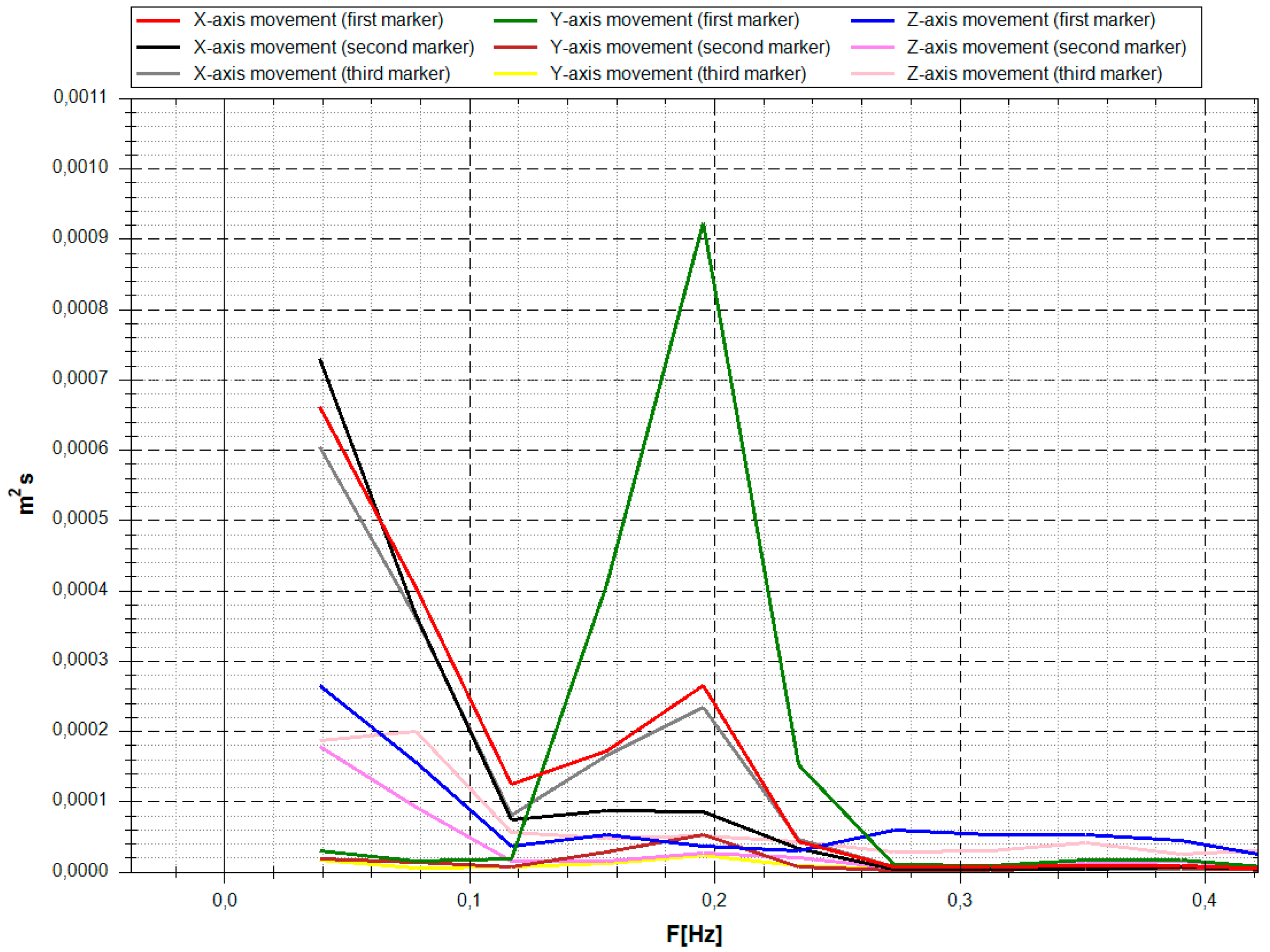
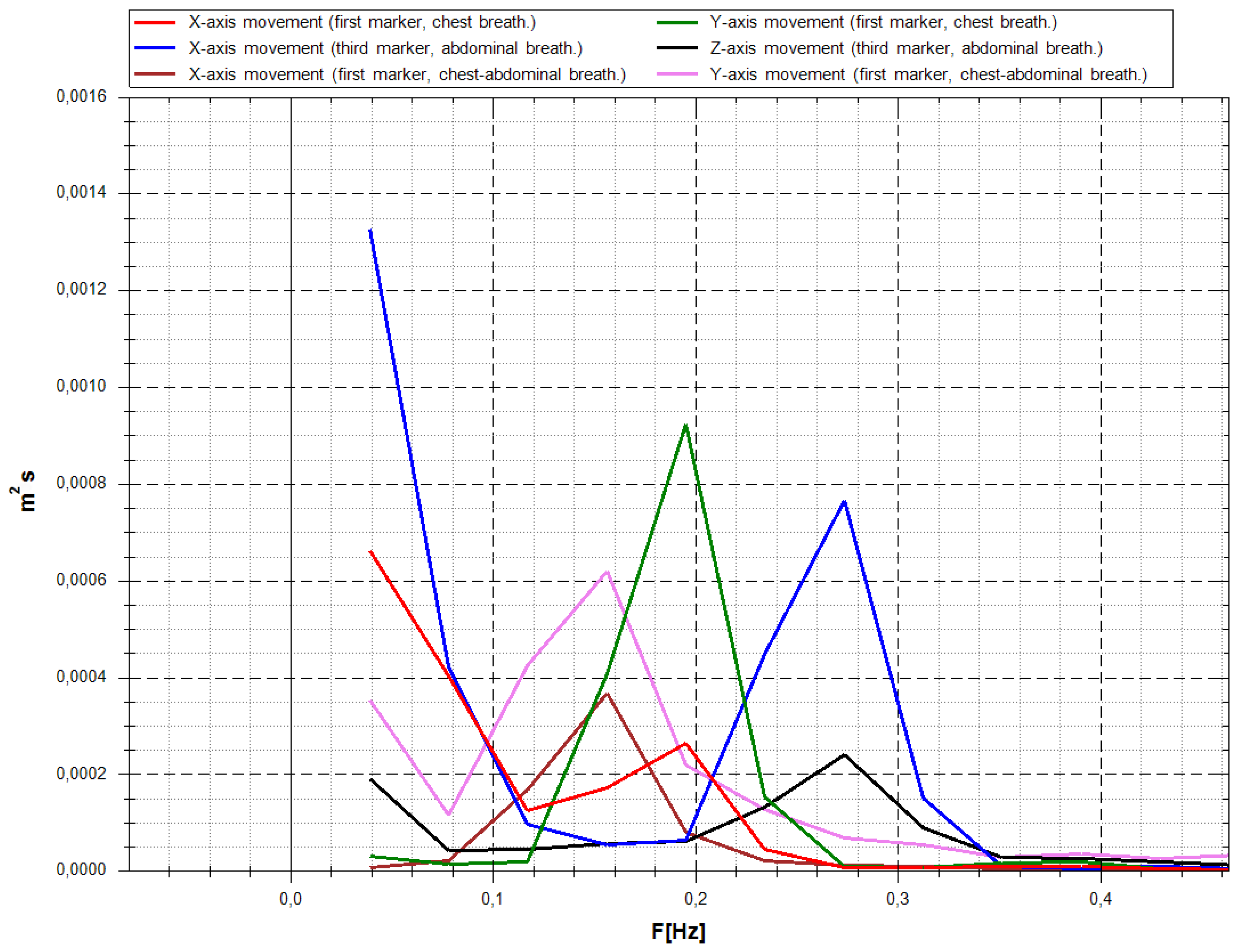
• RQ2. What is the difference in frequency responses of the person’s torso’s marker movement for different types of breathing?

The rest of the article is organized as follows. In Section 2, we discuss the equipment and methods we used to capture the breathing data, preprocess it, and describe the results of preliminary spectrum analysis of the data on different types of breathing. In Section 3, we show the results of training different machine learning models on this data and discuss their accuracy. In Section 4, we propose a two-stage algorithm for the detection of the kind of human breath, compare it to the previous models, and discuss our findings. Section 5 provides brief conclusions of our work.

2. Equipment and Methods of Capturing and Preparing Data

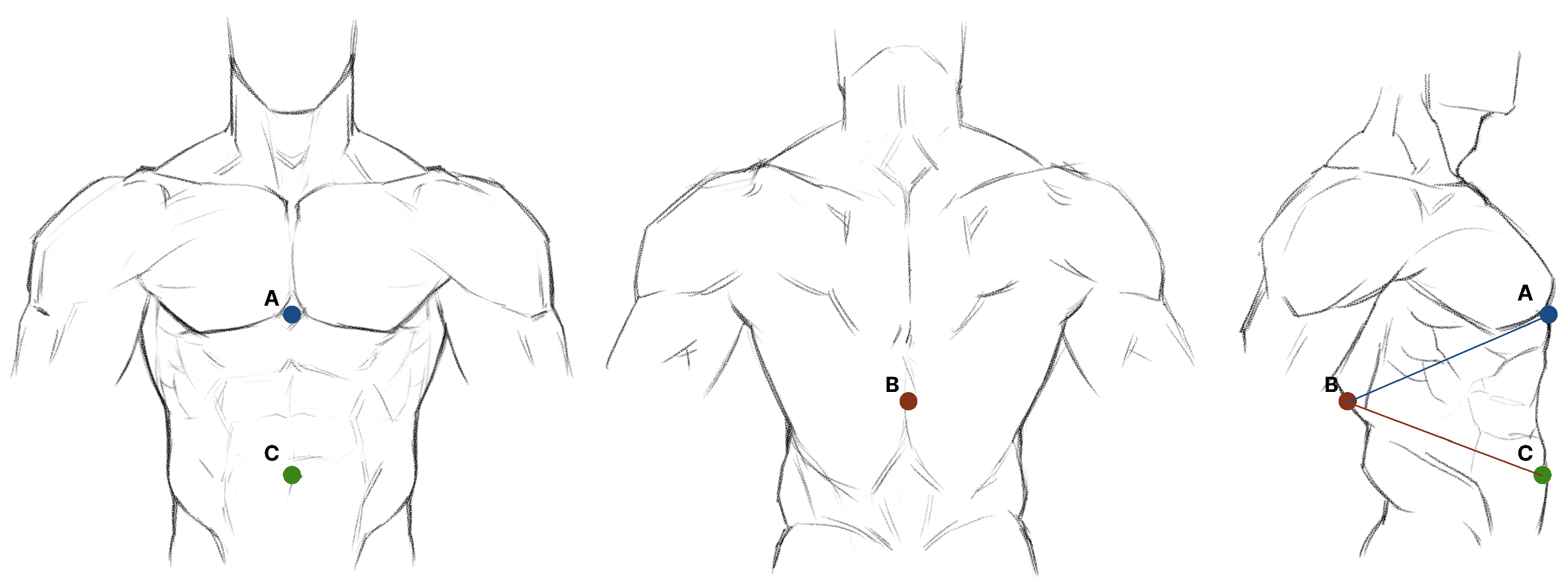
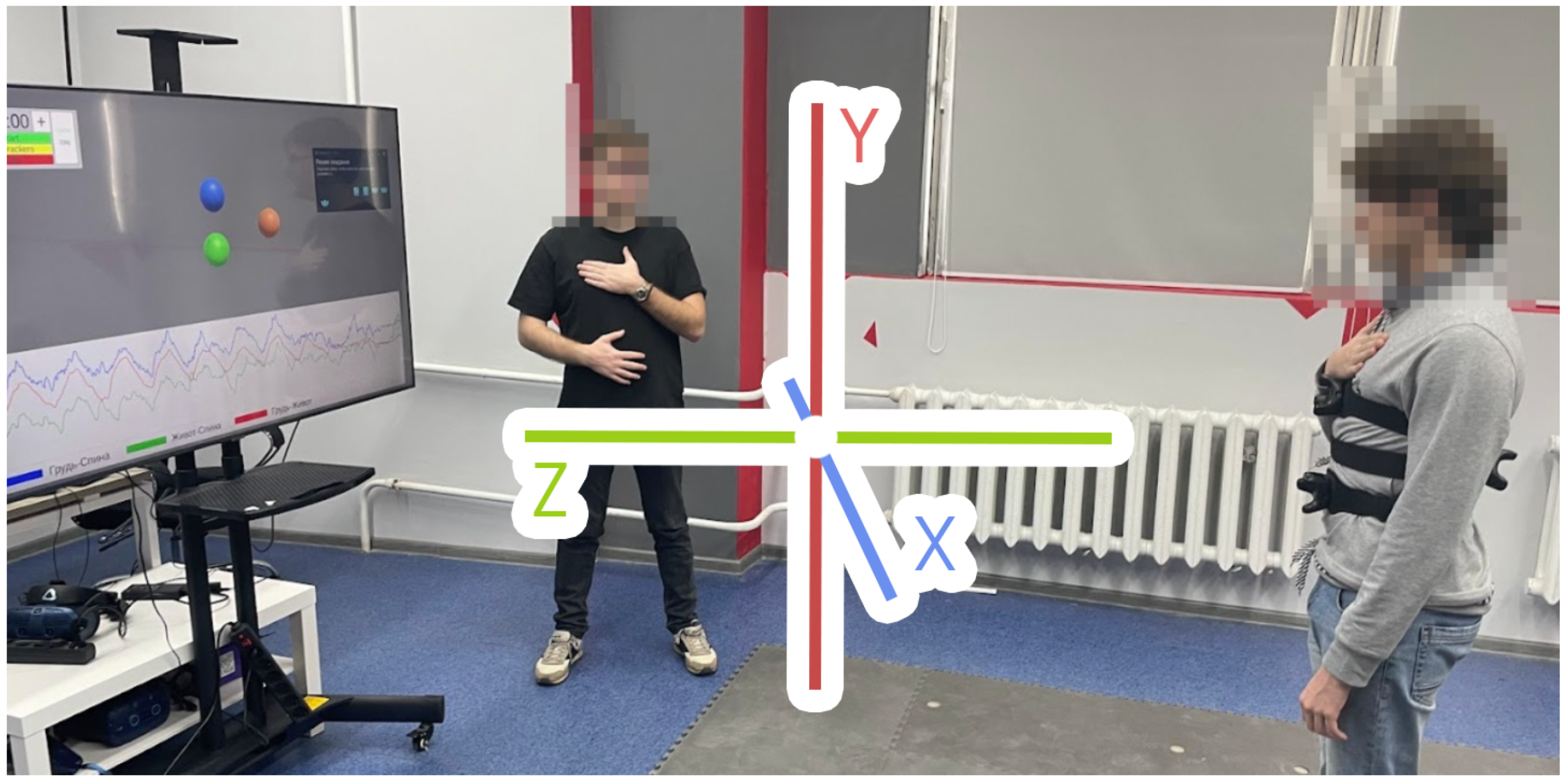
2.1. Motion Capture System

We chose the method of studying the dynamics of changes in the breathing pattern based on the motion capture system with subsequent signal processing as a part of the classification task [19,20,21].

The choice of motion capture system is important because one of our chief goals was wide accessibility of the products based on our results. There are various types and classes of motion capture systems, which differ in price, environment configuration, and complexity of use [22]. Based on a comparative analysis, the VIVE Tracker 3.0 hybrid inertial-optical motion capture system was chosen due to its price, accuracy, and low space requirements, which makes it possible to use it in small apartments. The configuration consists of the following elements:

• Three VIVE Tracker markers (3.0) (the minimum number required to track the movements of the chest and abdomen);
• Three waist elastic belts with fasteners for markers;
• Two SteamVR Base Stations 2.0.

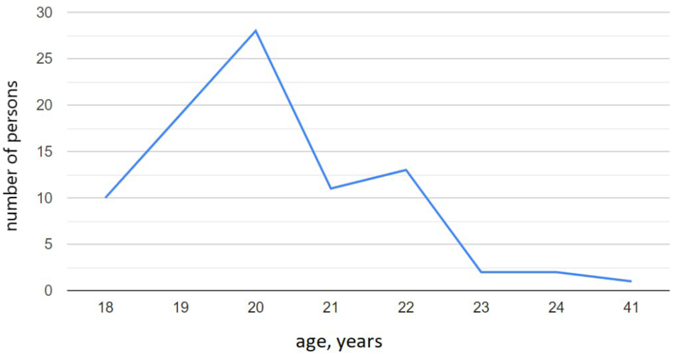
The system gives each marker six output values. Three of the six indicators reflect their positioning in three-dimensional space $(x,y,z)$ relative to the internal local space; the remaining three are the rotation angles relative to the same axes. Access to these markers is implemented through the API for Unity and Unreal Engine.

2.2. Study Design

The study involved 86 volunteers; the data were collected anonymously. The dataset contains information about the breathing of 67 men and 19 women. Of all the volunteers, 38 had COVID-19 (4 of them had lung damage), while 48 did not. The volunteers were of different ages, as shown in Figure 1.

Each participant provided the following questions:

• date of birth;
• biological sex;
• the last time interval of having COVID-19 (if any);
• percentage of lung damage;
• the presence of respiratory diseases at the time of data collection.

Three belts with fasteners for markers were attached to the participant. The fasteners were located on the xiphoid process of the sternum, between the 9th and 11th thoracic vertebrae, and above the navel. The belts were tightened moderately to allow comfortable breathing of the participant, but not too loosely so that the markers remained in place.

The scheme of attaching markers to the participant’s body is shown in Figure 2 [19].

The special software was developed to record the results from the motion capture system, marked timestamps, and the data about the volunteer.

Each of the markers tracks its own position in space and transmits the received information to the program for data collection. Thus, the data from one marker represent the change of its three spatial coordinates with time. The output of the data collection program is two files in the tsv format. The first file contains information about the participant, and the second file contains records of changes in the position of the marker and changes in the electrical activity of the muscles relative to time.

The participants were asked to breathe for a minute without any special requirements after attaching the sensor and markers. This test is needed to record the type of breathing common to the participant. After that, the participant was asked to breathe at his usual rate three times (a minute each) with different types of breathing—thoracic, abdominal, and mixed [23,24]. Before each session, a specially trained laboratory assistant explained to the participant how to breathe correctly for each type of breathing and visually verified that the volunteer had exactly the right type of breathing. For convenience and control, the volunteer could control the movement of the body with his palm so that the markers were not blocked.

Figure 3 shows how data collection happened. In relation to the participant, the axes were arranged as follows: the Y axis was directed upward, the Z axis was directed towards the person, and the X axis was directed to their left. These results were recorded for further processing.

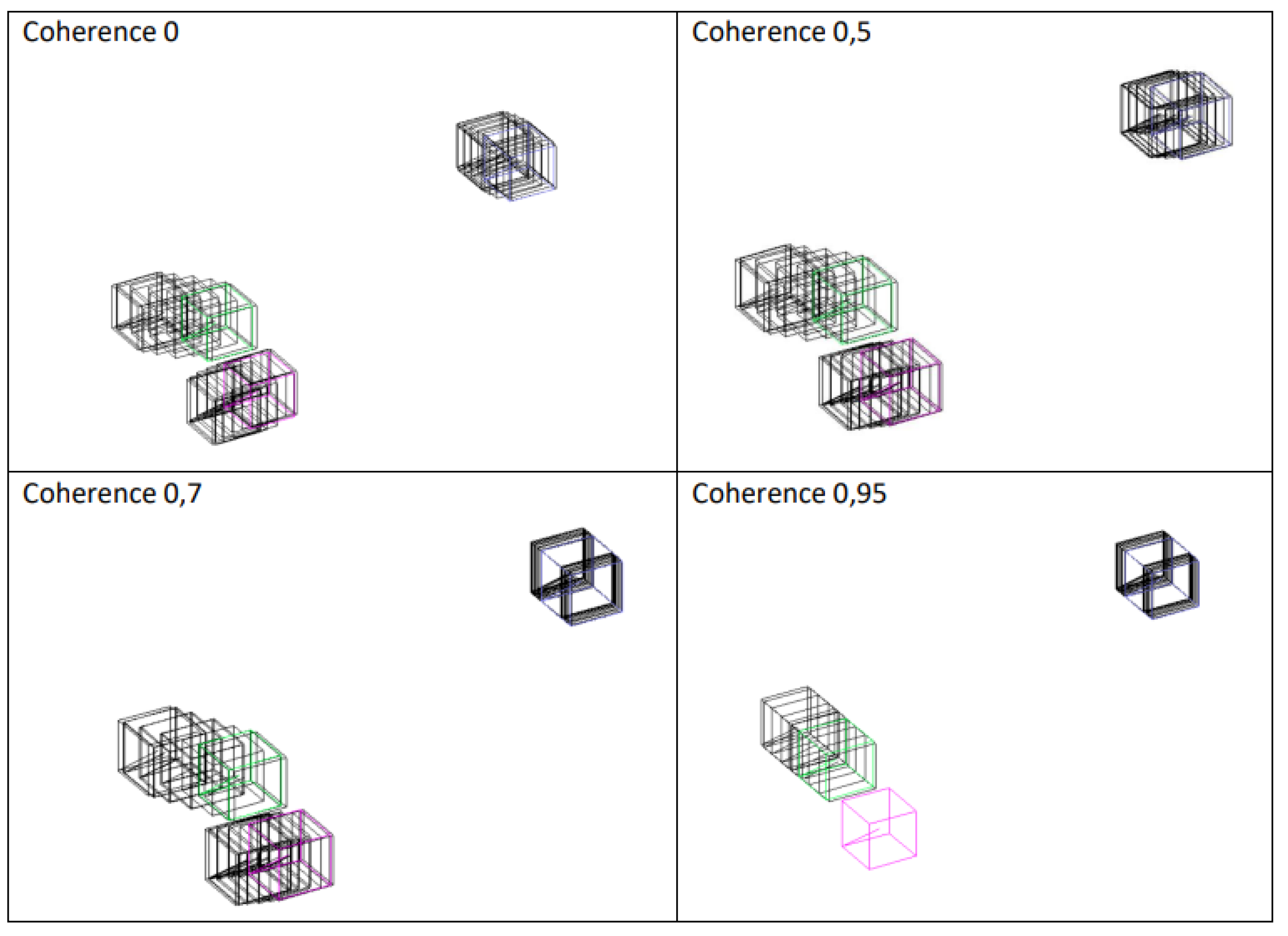
2.3. Data Preprocessing

The original data were preprocessed before being passed to the model. First, it was necessary to ensure that each participant had four files with measurements of various types of breathing (standard, thoracic, abdominal, and mixed). For six participants, we found that the same type of breathing was recorded more than once. Duplicate files were deleted. After that, it was essential to confirm that the measurement lasted no less than a minute in each file. Eight measurements lasting significantly less than a minute were found; they were removed as statistical outliers. It was also noticed that in some files, the fractional part of the numbers was separated by a comma instead of a dot. Such data were converted to a single format: the separation of the integer and fractional parts of the number by the dot symbol.

The remaining statistical outliers were searched using the interquartile range method. The interquartile range is the difference between the third (Q3) and the first (Q1) quartiles of the sample. This value helps estimate the spread of 50% of the sample elements without taking into account outliers [25,26,27]. Statistical outliers were records for which the frequency or amplitude values were 1.5 times greater or 1.5 times lower than the interquartile range (IQR), i.e., all the records that had a frequency or amplitude value less than the corresponding lower limit or upper limit according to (1).

$$\begin{array}{c}\hfill IQR=Q3-Q1\\ \hfill Lowerlimit=Q1-1.5·IQR\\ \hfill Upperlimit=Q3+1.5·IQR\end{array}$$

(1)

In addition, all numerical characteristics were scaled using the StandardScaler from the scikit learn (sklearn) Python library before being passed to the model for training; all categorical characteristics were represented appropriately using the get_dummies method from the Python Pandas library. The dataset was divided into training (60% of records) and test (40% of records) samples, using the train_test_split method from the Python scikit learn (sklearn) library.

We chose the ratio of training and test samples based on [28], which supposed using 60% of the original data for the training sample, 20% for the validation sample, and 20% for the test sample; those recommendations are suitable for the data volume we had. The validation sample is used when the model independently selects optimal hyperparameters, which was not done in our study. Therefore, 60% of the data was allocated for the training sample. The training and test samples data do not intersect: the separation was performed before the training. The data were balanced in the test and training samples because the “stratify” parameter was used in the train_test_split method. That method performs a random split: it shuffles the sequence of all the data to eliminate the factor of models’ selection of false (“biased”) features associated with the training data sequence.

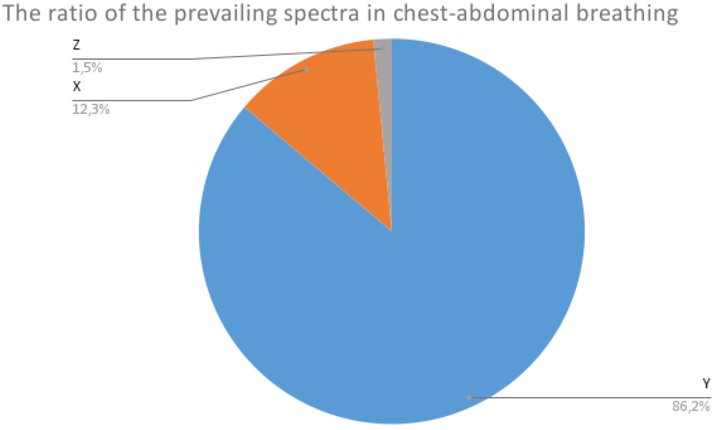
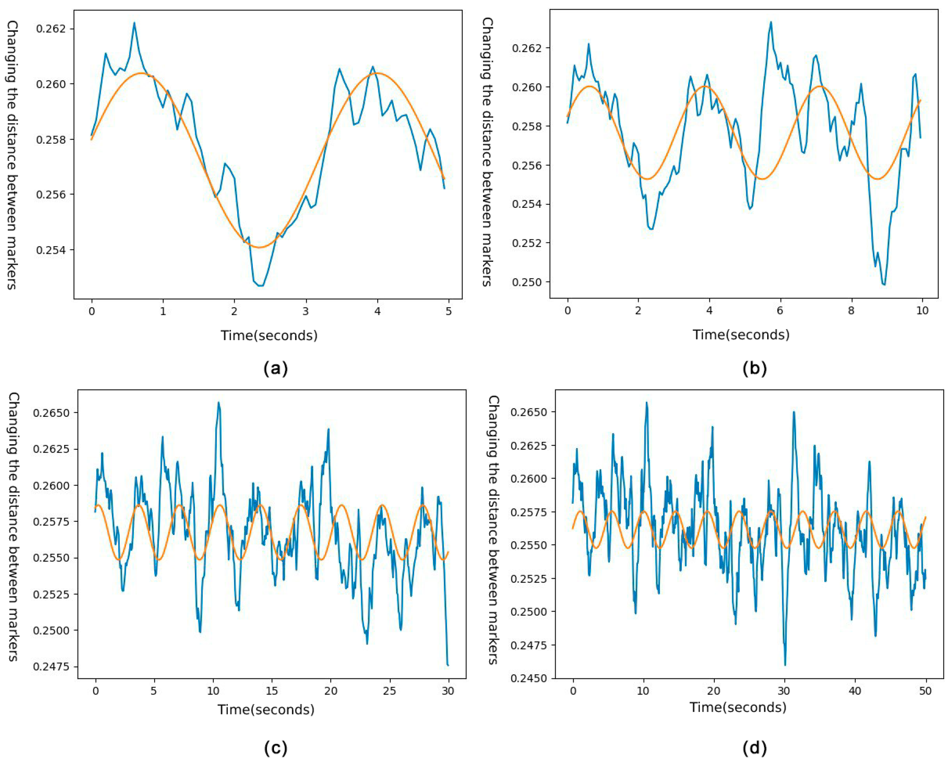
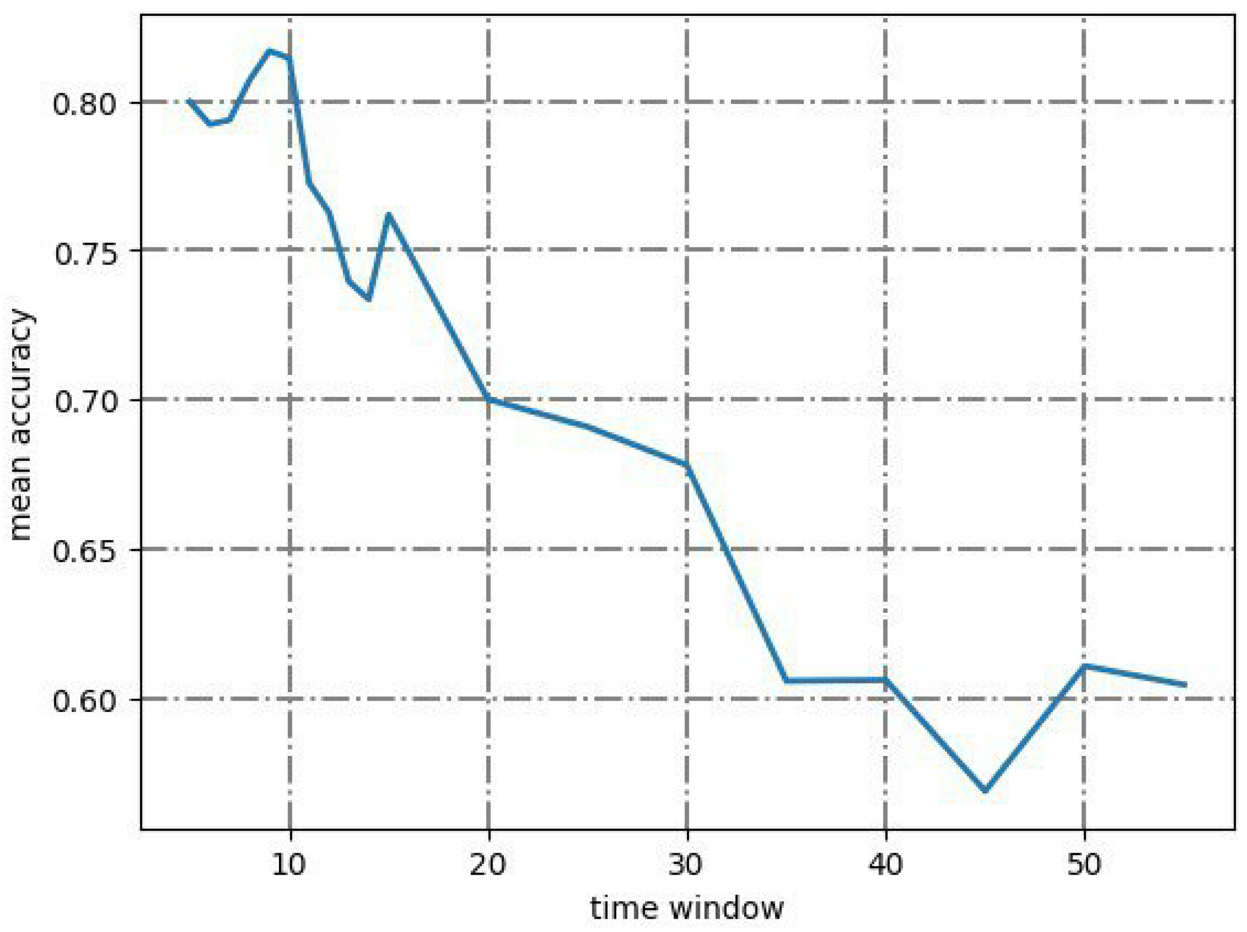
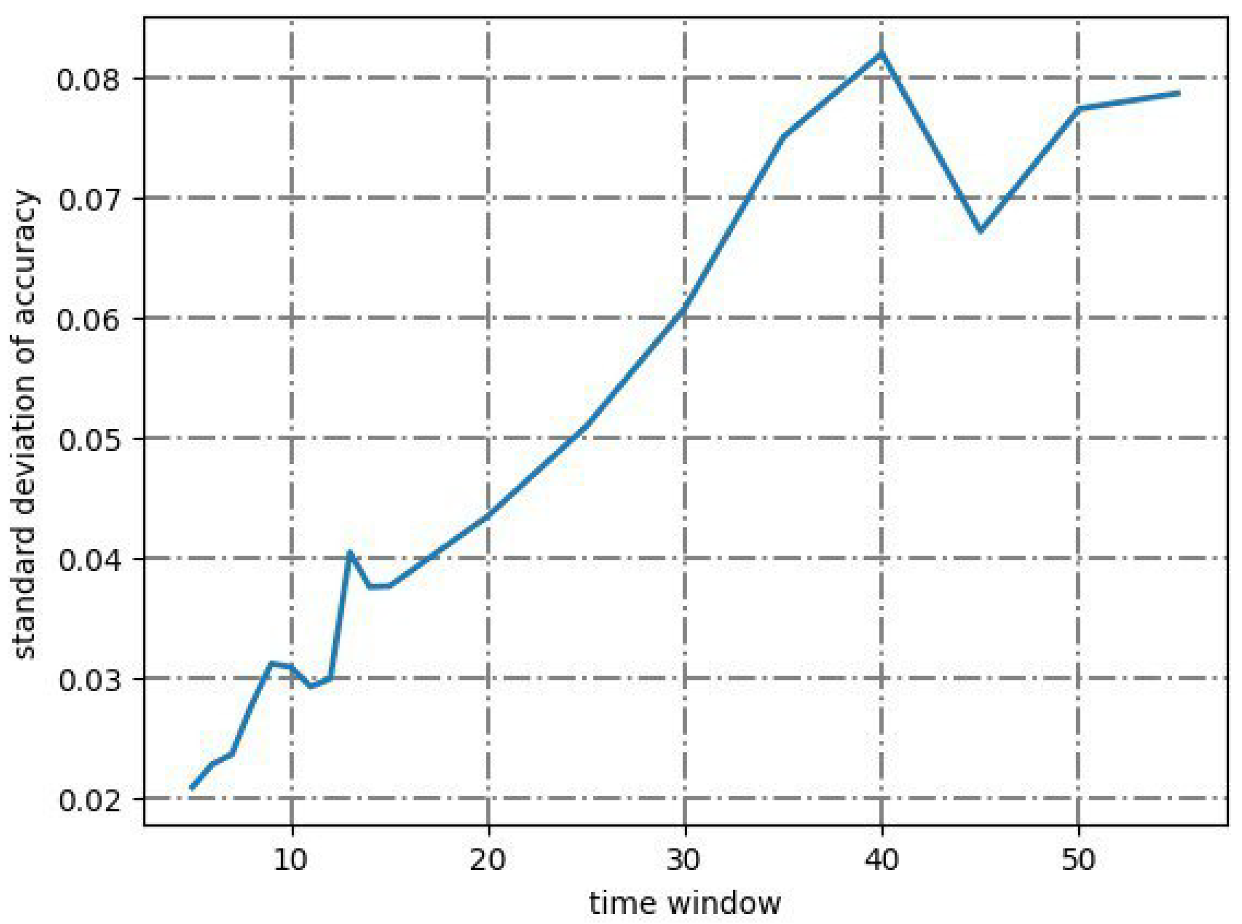
2.4. Signal Spectrum Analysis

The accuracy of the classical ML models, when trained on kinematic data, was not good. This can be explained by the lack of training data. Since experimentation is a lengthy process, the researchers tried to approach this problem from the side of classical signal processing problems and began to analyze the spectral characteristics obtained from existing data [29,30].

We conducted the study using the software preprocessor for forming and solving the nonlinear dynamics equations from the FRUND package [31], which was developed at Volgograd State Technical University. The example of transforming the coordinates of the autospectrum power for one complete breathing cycle is presented in Figure 4.

The analysis of the autospectrum power signal revealed the patterns shown in Figure 5.

As the diagrams show, most of the participants demonstrated a significant predominance of changes in the Y coordinate of the first (thoracic) marker during thoracic breathing; also, changes in the Z coordinates of different markers were also predominant.

For thoracic breathing, the frequency ranges of the predominant spectra were divided according to Figure 6. Most of the spectral peaks were in either the 0.15–0.17 Hz or 0.19–0.21 Hz ranges.

The spectral analysis of abdominal breathing revealed the following patterns: patterns for the predominant spectra are presented in Figure 7; changes in the X coordinates of the third (abdominal) and the first markers were predominant for most of the participants.

For abdominal breathing, the frequency ranges of the predominant spectra were divided as shown in Figure 8. All values fall within the range of values presented in the figure with an accuracy of 0.05 Hz. According to this diagram, there is an intersection of groups of frequencies of abdominal breathing with groups of thoracic breathing. Therefore, it is impossible to reliably discern the type of breathing by the frequency group.

For mixed (diaphragmatic-costal) breathing, only changes in the coordinates of the first (thoracic) marker were predominant, mostly the Y coordinate. The correlation of the predominant spectra is presented in Figure 9.

When analyzing frequencies, there is also an intersection with other types of breathing in frequency groups. This indicates the impossibility of using frequency groups as the only criterion for determining the type of breathing. The correlation of the predominant frequencies in chest-abdominal breathing is presented in Figure 10.

Figure 11 shows an example of the intersection of the predominant spectra for different types of breathing. This example is relatively good for determining the breathing type because all three types of breathing can be distinguished on this graph. Even though the common predominant spectra can be determined by the type of marker coordinate change, one can distinguish types of breathing by frequency groups. However, as mentioned earlier, the frequency groups intersect as do the groups of changes in the predominant coordinates of the markers. Therefore, it is impossible to take the combination of the predominant frequency and the predominant spectrum as an unambiguous criterion for determining the type of breathing.

The following patterns were revealed during the primary visual analysis of the respiration spectra, which are presented in Figure 12. In the decision tree diagram for choosing the type of breathing depending on the predominant spectrum, not all choices lead to unambiguous answers. It can be concluded that the construction of an algorithm based on the spectra does not allow the type of breathing to be reliably determined.

We conducted a mutual spectral analysis of the breathing types to solve these problems. The cinegrams of mutual spectral analysis for several volunteers for all three types of breathing are shown in Figure 13 and Figure 14. In these figures, the model of the first (thoracic) marker is shown in green, the second (dorsal) marker in blue, and the third (abdominal) marker in magenta.

Figure 13 presents mutual spectral analysis cinemagraphs for thoracic breathing.

Figure 14 presents similar cinegrams for abdominal breathing, and Figure 15 shows them for the mixed type of breathing.

Therefore, the mutual spectral analysis helped identify the key characteristics of different types of breathing. The value of these characteristics determines the result of prediction, making it possible to create more accurate models.

3. Coordinate-Based Machine Learning Models

Several mathematical models, including neural networks, were trained on the database of marker kinematics, which were obtained after postprocessing.

We started by calculating more characteristics to increase the classification accuracy.

The first characteristics we used were the vector breathing rates in projections on the coordinate axes. We selected the velocity of the thoracic marker relative to the dorsal marker and the velocity of the abdominal marker relative to the dorsal marker because they conveyed meaningful information. The velocity of the thoracic marker relative to the abdominal marker or vice versa can be ignored because they move in the same direction during breathing. According to the obtained vector velocities, the corresponding scalar velocities were calculated for each unit of measurement time between the above markers.

We also calculated pairwise distances between all three markers. The distances between the markers were calculated as the length of the vector according to the markers’ coordinates. Graphs of changes in the distances between markers during the measurement process for various types of breathing are presented in Figure 16.

Another important characteristic is the average respiratory rate. It was calculated as the number of inhalation/exhalation cycles’ per time interval divided by that time interval. The distance between two adjacent maxima was considered for the inhalation/exhalation cycle. The seasonality function of the time series was used to calculate it. We also calculated the mean breathing amplitude as the arithmetic average of the distances between the maxima and the minima closest to them [32].

The next step was selecting the machine learning models and parameters for them. The parameters were selected by applying the cross-validation method [33] and manually adjusting them. It required splitting the original sample into N subsamples. The model was trained N times on $N-1$ subsamples and tested on the remaining subsample, which was different each time. Machine learning was performed for each combination of parameters, and the results were compared to find the best-performing parameters. We performed cross-validation using the GridSearchCV class from the scikit learn (sklearn) Python library.

3.1. Decision Tree Model

A decision tree consists of nodes called “leaves” and “branches”. “Leaves” contain the values of the target variable, while “branches” contain the characteristics (attributes) on which the target variable depends [34,35,36]. The following characteristics were used as the input of this model: the sex of the participant; whether they were infected with COVID-19; the presence of lung damage; the percentage of lung damage; the average respiratory rate; the average amplitude of respiration. The model gave a string containing the name of the type of breathing at output. The parameters presented in

Table 2. Hyperparameters for decision tree classifier.

Hyperparameter	Short Description	Value
criterion	A function that evaluates the quality of division at each node of the decision tree.	“gini”
splitter	The strategy used to select a specific division from the set at each node, taking into account the estimates obtained from the function specified in the criterion parameter.	“best”
max_depth	Maximum depth of the decision tree.	5
min_samples_split	The minimum number of samples required to split a node of the decision tree.	2
min_samples_leaf	The minimum number of samples required to form a “leaf”.	1
max_features	The number of functions to consider when searching for the best partition.	3
random_state	Setting the fixed state of the random component.	12

were set as hyperparameters. This model gave an accuracy score of 0.510.

3.2. Random Forest Model

This model consists of a set of decision trees, where each tree is built either on the basis of the entire input sample or on its random part. The best partition is selected either from all the data or from its subset when selecting nodes in a tree [37]. The following characteristics were used as the input of this model: the sex of the participant; whether they were infected with COVID-19; the presence of lung damage; the percentage of lung damage; the average respiratory rate; the average amplitude of respiration. The output was the type of breathing. The parameters presented in

Table 3. Hyperparameters for random forest classifier.

Hyperparameter	Short Description	Value
criterion	A function that evaluates the quality of division execution at each node of the decision tree.	“gini”
n_estimators	The number of decision trees in a random forest.	10
max_depth	Maximum depth of decision trees.	5
min_samples_split	The minimum number of samples required to split a node of the decision tree.	2
max_features	The number of functions to consider when searching for the best partition; when “sqrt”: $max\_features=\sqrt{n\_features}$.	“sqrt”
bootstrap	Indicates whether it is necessary to split the initial sample into several random subsamples when training trees.	True
random_state	Setting the fixed state of the random component.	12

were set as hyperparameters. Using this model resulted in an accuracy score of 0.531.

3.3. K-Neighbors Model

This model determines the class for the data by comparing the classes of other nearest neighbors. The essence of choosing the final class is to choose the one that prevails among k neighbors [38]. The following characteristics were used as the input of this model: the sex of the participant; whether they were infected with COVID-19; the presence of lung damage; the percentage of lung damage; the average respiratory rate; the average amplitude of respiration. The model gave a string containing the name of the type of breathing at output. The parameters presented in

Table 4. Hyperparameters for K-neighbors classifier.

Hyperparameter	Short Description	Value
n_neighbors	Number of neighbors.	4
weights	The weight function used in prediction.	‘distance’
metric	A metric used to calculate the distance to neighbors.	‘minkowski’

were set as hyperparameters. This model gave an accuracy score of 0.408.

3.4. Catch 22 Classifier Model

This model captures a diverse and interpretable time series signature in terms of their properties, including linear and nonlinear autocorrelation, sequential differences, value distributions and outliers, oscillation scaling properties, etc. It builds the estimate using transformed data [39]. The following characteristics were used as the input of this model: the time series containing marker coordinates, the calculated vector and scalar velocities, and the distances between markers. The model gave a string containing the name of the type of breathing at output. The parameters presented in

Table 5. Hyperparameters for Catch 22 classifier.

Hyperparameter	Short Description	Value
outlier_norm	Normalization of each sequence during two additional Catch 22 functions.	True
n_jobs	Parallelization of calculations into multiple threads.	−1
random_state	Setting the fixed state of the random component.	12

were set as hyperparameters. This model gave an accuracy score of 0.630.

3.5. Rocket Classifier Model

The rocket classifier is a time series classification model directly based on the random transformation of the convolutional kernel [40,41]. This model uses the methodology of transforming data from time series using convolutional kernels. The rocket model computes two aggregate objects from each kernel and convolutions of the objects. The following characteristics were used as the input of this model: the time series containing marker coordinates, the calculated vector and scalar velocities, and the distances between markers. The parameters presented in

Table 6. Hyperparameters for rocket classifier.

Hyperparameter	Short Description	Value
num_kernels	Number of kernels.	500
n_jobs	Parallelization of calculations across multiple threads.	−1

were set as hyperparameters. That model gave an accuracy score of 0.459.

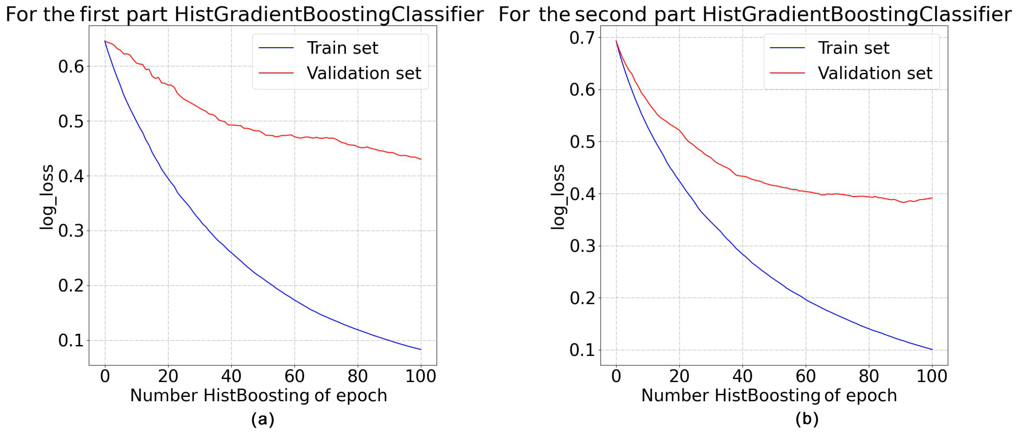
3.6. Hist Gradient Boosting Classifier

This is a model that uses gradient boosting and decision trees. The main idea of the algorithm is the sequential application of the predictor in such a way that each subsequent model minimizes the error of the previous one [42]. The following characteristics were used as the input of this model: the time series containing marker coordinates, the calculated vector and scalar velocities, and the distances between markers.

Table 7. Model hyperparameters.

Hyperparameter	Short Description	Value
random_state	Setting the fixed state of the random component.	15
learning_rate	Learning rate.	1
max_depth	Maximum depth of the decision trees.	15
loss	The loss function that the model minimizes during the boosting process.	‘log_loss’

presents the hyperparameters of the trained models. That model gave an accuracy score of 0.418.

To achieve the goal of this study, it is essential to consider individuals’ physiological characteristics. For some people, these characteristics can be mistaken for outliers when training the model. We chose logistic loss (see (2) below) as the loss function for training our models. It is often used in machine learning practice because of its resistance to outliers [28].

3.7. Other Models

We also attempted to train the CNN classifier, FCN classifier, and MLP classifier [43,44] using the following characteristics as the input: the time series containing marker coordinates, the calculated vector and scalar velocities, and the distances between markers. Their accuracy scores were in the range of 0.33–0.35, which is comparable to random guessing.

4. Two-Stage Method for Determining the Type of Human Breathing

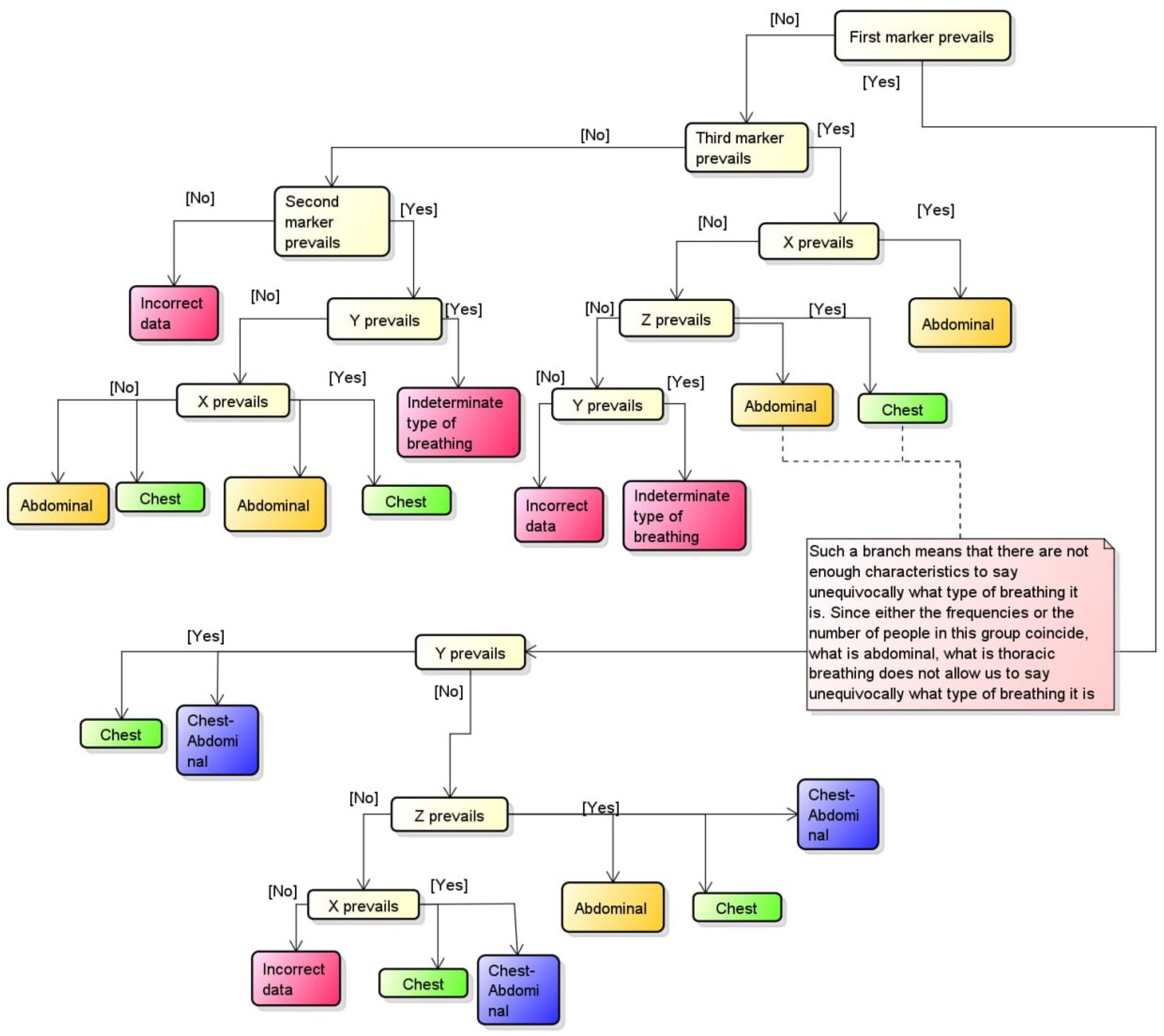
4.1. Algorithm

When charting distances between two markers, it was noticed that they resembled sine waves.The main idea of the proposed approach was to select sine waves that model the shape of the original graphs.

Figure 17 shows graphs of the change in distance between the thoracic and abdominal markers and the assumed sine wave. It can be seen from this figure that the graph of the modeling sine wave adheres to the shape of the graph of the change in distance between the markers quite well.

Because the results described above demonstrated that discerning between the three types of breathing is difficult, we decided to divide the process into two stages of binary classification: the first was discerning mixed breathing from two other kinds of breathing; the second step was discerning thoracic and abdominal breathing patterns if necessary. This improved the process of determining the mixed type of breathing by using a model especially dedicated to this problem.

The input data for our algorithm consist of multiple lines representing different time steps. Each line contains the spatial coordinates of three sensors at a certain point in time, namely, the chest sensor denoted as ($X_1,Y_1,Z_1$), the back sensor denoted as ($X_2,Y_2,Z_2$), and the abdominal sensor denoted as ($X_3,Y_3,Z_3$).

We used the function $savgolFilter(data,windowSize,polynomialOrder)$ (implemented using the savgol_filter function from the scipy library) to perform Savitzky–Golay filtering on the data; windowSize is the size of the window used for filtering, and polynomialOrder is the order of the polynomial used in the filtering process. The function returns the filtered data as an array of the same length as the input data. The function $fftfreq\left(f\right(t\left)\right)$ (implemented using the fft and fftfreq functions from the numpy library) is used to perform the Fourier Transform on a given function $f\left(t\right)$ and returns an array of frequencies. The function $curveFit\left(f\right(t),data)$ (implemented using the curve_fit() function from the scipy library) is used to fit a function f to a given dataset using nonlinear least squares. The function f can be provided with initial guesses for each of its parameters. The output of the $curveFit$ function is a tuple of the best-fit parameters for the function f.

Algorithm 1 uses the following notation: $d_{ij}$—distance between markers i and j; ${d^{\prime }}_{ij}$—distance between markers i and j with Savitzky–Golay filtering applied; $sin{w}_{ij}$—the sine wave in the form (2), which was fitted to ${d^{\prime }}_{ij}\left(t\right)$; $A_{ij}$ and ${A^{\prime }}_{ij}$—the amplitude of $sin{w}_{ij}$ (initial guess and the best-fit value, respectively); $w_{ij}$ and ${w^{\prime }}_{ij}$—the angular frequency of $sin{w}_{ij}$ (initial guess and the best-fit value, respectively); ${\phi }_{ij}$ and ${{\phi }^{\prime }}_{ij}$—the phase of $sin{w}_{ij}$ (initial guess and the best-fit value, respectively); $c_{ij}$ and ${c^{\prime }}_{ij}$—the offset of $sin{w}_{ij}$ (initial guess and the best-fit value, respectively); $X\leftarrow Y$ is the operator appending a new value (set of values) Y to a list X.

$$y=Asin(\omega t+\phi )+c,$$

(2)

Algorithm 1 Algorithm of determining the type of human breath

1: function TypeOfBreath($MarkersFile$) 2:    for all $i,j\in \{1,2,3\},i<j$ do: 3:       for all t in $MarkersFile$ do 4:        $d_{ij}^t=\sqrt{{(X_j^t-X_i^t)}^2+{(Y_j^t-Y_i^t)}^2+{(Z_j^t-Z_i^t)}^2}$ 5:        $d_{ij}\leftarrow d_{ij}^t$ 6:       end for 7:       ${d^{\prime }}_{ij}=savgolFilter(d_{ij},15,5)$ 8:       $A_{ij}=\sqrt{2}std\left({d^{\prime }}_{ij}\right)$ 9:       $c_{ij}=\overline{{d^{\prime }}_{ij}}$ 10:     $f_{ij}=fftfreq\left({d^{\prime }}_{ij}\right)\left[1\right]$ 11:     ${\omega }_{ij}=2\pi f$ 12:     ${\phi }_{ij}=0$ 13:     $sin{w}_{ij}\left(t\right)=A_{ij}sin({\omega }_{ij}t+{\phi }_{ij})+c_{ij}$ 14:     $<{A^{\prime }}_{ij},{c^{\prime }}_{ij},{f^{\prime }}_{ij},{{\omega }^{\prime }}_{ij},{{\phi }^{\prime }}_{ij}>=curveFit(sin{w}_{ij}\left(t\right),{d^{\prime }}_{ij})$ 15:    end for 16:    for all $i,j\in \{1,2,3\},i<j$ do: 17:     $params\leftarrow <{A^{\prime }}_{ij},{c^{\prime }}_{ij},\frac{1}{{f^{\prime }}_{ij}},{{\omega }^{\prime }}_{ij},{{\phi }^{\prime }}_{ij}>$ 18:    end for 19:    $params\leftarrow \frac{{A^{\prime }}_{12}}{{A^{\prime }}_{23}},\frac{{A^{\prime }}_{12}}{{A^{\prime }}_{13}},\frac{{A^{\prime }}_{23}}{{A^{\prime }}_{13}},\frac{{c^{\prime }}_{12}}{{c^{\prime }}_{23}},\frac{{c^{\prime }}_{12}}{{c^{\prime }}_{13}},\frac{{c^{\prime }}_{23}}{{c^{\prime }}_{13}},\frac{{f^{\prime }}_{12}}{{f^{\prime }}_{23}},\frac{{f^{\prime }}_{12}}{{f^{\prime }}_{13}},\frac{{f^{\prime }}_{23}}{{f^{\prime }}_{13}}$ 20:    $params‘=stdScale\left(params\right)$ 21:    $predictedType=mode{l}_1.predict(params‘)$ 22:    if $predictedType==$ mixed_type then 23:     return $mode{l}_2.predict(params‘)$ 24:    else 25:     return $predictedType$ 26:    end if 27: end function

One of the important hyperparameters for training a machine learning algorithm for determining the type of human breathing is the time window (the amount of data supplied to the algorithm for one run). We analyzed the overlay of the sine wave $sin{w}_{ij}$ on the graph of the distance function between the two sensors ${d^{\prime }}_{ij}$ (i.e., the breathing type graph). The graphs shown in Figure 18 present the results of the transformation of the function ${d^{\prime }}_{ij}$ using the least squares method [45] for time windows of 5, 10, 30, and 50 s. You can see that the smaller the window, the better the $sin{w}_{ij}$ function describes the dataset. Based on the graphs, the most appropriate window sizes are 5 and 10 s (when the $sin{w}_{ij}$ graph almost entirely coincides with the ${d^{\prime }}_{ij}$ graph).

To find the optimal time window size, we conducted an experiment to determine how the time window affects the accuracy of the trained model. We fixed the other hyperparameters and varied the time window from 5 to 60 s: for the values in the interval 5–15 s, the measures were taken each second; for the interval 16–60 s, the measures were taken each 5 s. As the accuracy of the trained model is a random value, we performed 100 measurements for each time window size and calculated the mean value. Figure 19 and Figure 20 present the dependencies of the mean accuracy and standard deviation on the window size.

The graph in Figure 19 shows the highest accuracy achieved in 5–12 s. We hypothesize that the small time window sizes produced better accuracy because they contained fewer cycles of breathing and so lower the chance of a person performing different types of breathing in one data sample.

Figure 20 shows the standard deviation of the model accuracy. While it grows from 5 to 12 s, that increase is far lower than the increase of the mean accuracy, so we decided that 10 s was the best time window to train machine learning models for determining the type of human breathing.

We trained the selected classifiers using a two-step algorithm. We used the following metrics to assess the quality of the trained models: accuracy, precision, recall, and F1-measure [46,47,48], training and running time, and the value of log_loss loss function.

The measurements were made on the Acer Aspire 5 A515-45G-R92Q computer with the following hardware:

• AMD Ryzen 7 5700U 8x 1.80 GHz;
• AMD Radeon™ RX 640;
• 16 Gb RAM 3200 MHz.

The results are presented in

Table 8. Model quality evaluation results.

Model Kind	Number of Models	Accuracy	Precision	Recall	F1-Measure	Training time, s	Working Time, s	log_Loss (Logistic Loss)
Random Forest Classifier	1	0.53	0.5	0.54	0.47	0.018	0.002	8.67
Decision Tree Classifier	1	0.51	0.46	0.51	0.46	0.004	0.001	13.24
Catch 22 Classifier	1	0.63	0.65	0.63	0.64	8.926	8.665	0.94
Rocket Classifier	1	0.46	0.45	0.46	0.46	11.507	5.437	18.68
K-Neighbors Classifier	1	0.41	0.38	0.41	0.36	0.006	0.001	10.8
Hist Gradient Boosting Classifier	1	0.42	0.51	0.42	0.37	0.324	0.009	4.22
Random Forest Classifier	2	0.46	0.46	0.46	0.46	0.047	0.485	6.78
Decision Tree Classifier	2	0.52	0.52	0.52	0.52	0.004	0.11	13.21
Catch 22 Classifier	2	0.57	0.57	0.57	0.57	19.02	34.609	0.96
Rocket Classifier	2	0.48	0.48	0.48	0.48	35.318	64.687	17.83
K-Neighbors Classifier	2	0.4	0.4	0.4	0.4	0.005	0.407	7.89
Hist Gradient Boosting Classifier	2	0.81	0.83	0.82	0.82	0.875	0.75	1.98

. The best accuracy was achieved by hist gradient boosting classifier.

The $log\_loss$ metric was used to estimate the probabilistic results of model prediction ($predict\_proba$, a probabilistic estimate of each classifier class); i.e., we minimized the logarithmic difference between the predicted probabilities and the actual labels. The model strives to minimize that metric, so the smaller it is, the better the accuracy of the model prediction. The metric was calculated using the formula (3):

$$log\_loss=-\frac{1}{N}\sum _{i=0}^{N-1}\sum _{k=0}^{K-1}{y}_{i,k}log{p}_{i,k},$$

(3)

where N is the test sample size, K is the number of classes, Y is the test sample, $y_{i,k}$ is the actual value of the considered class, P is the matrix of probability estimates of each class, and $p_{i,k}$ is the probability estimate of the considered class [49].

Figure 21 shows the loss function depending on the training epoch for two hist gradient boosting classification models. There is no model overfitting as the graphs show because both functions tend to zero, albeit slowly.

The main quality evaluation metrics were accuracy and recall. We chose them as the primary metrics because accuracy allows us to assess how correctly our model predicts all the types of breathing, and recall allows us to monitor the wrong results for mixed breathing, which is of particular interest to us. Table 8 clearly shows that the proposed two-model algorithm with hist gradient boosting classifier produced the best results, significantly outperforming other machine learning methods; these results are good enough to be used in practical applications.

4.2. Discussion

Research concerning determining the type of human breath has a relatively wide range of aims: from diagnosing diseases via human breathing to the measurement of respiratory rate and counting the number of inhalations per minute.

The model developed by Yanbin Gong et al. [16] can detect the thoracic type of breathing with a 95% accuracy using breathing belts. This exceeds the accuracy of our model, but this model only recognizes one type of breathing: thoracic (diaphragmatic). This severely limits its use, while the model we proposed in this study attempts to classify three types of breathing at once: thoracic, abdominal, and mixed.

It must also be noted that, according to [50], the model we developed uses sensors that cost significantly less than the competitive models. Another advantage of the proposed method is the required minimum free space: the proposed system requires only 3 square meters, while other motion capture systems require at least 10-20 square meters. While this limits the amount of data we analyze and so the accuracy of the model, it can be used in home environments, which is important for rehabilitation.

RQ1. Can kinematic data taken from key points of the torso be used to determine the person’s characteristic type of breathing with satisfactory accuracy for respiratory rehabilitation?

One of the goals of this study was to determine the viability of developing a software system to determine the human breathing type based on the placement of three sensors fixed on the key points of the torso: the xiphoid process, the point on the back between the 9th and 11th thoracic vertebrae, and the point located above the navel. According to interviewed rehabilitation experts, at least three breathing cycles out of four must be correctly determined for effective rehabilitation. The best model trained in this study—a composite model of two hist gradient boosting classifiers—had an accuracy score of 0.81 for determining the breathing type, which meets the requirements (Table 8). We plan to research further possibilities of improving the quality of predictions using various machine learning models and expanding the dataset using additional EDA sensors, heart rate sensors, SpO${}_2$, a gyroscope, and an accelerometer. It is also planned to increase the dataset by gathering data from more people of various ages and genders.

RQ2. What is the difference of frequency responses of the person’s torso’s marker movement for different types of breathing?

According to the above diagrams in Figure 5, Figure 6, Figure 7, Figure 8, Figure 9 and Figure 10, most volunteers breathed in the frequency range of 0.15–0.30 breaths per second during thoracic breathing. The most characteristic frequency was 0.2. The frequency range for abdominal breathing was 0.156–0.312 breaths per second. The frequency of breaths increased, but not significantly. The most characteristic frequency was 0.273. When using the mixed breathing type, most frequency values were 0.11–0.24 breaths per second. The predominant frequency became 0.156 breaths per second. We encountered many frequency groups common to all the breathing types, which made it difficult to determine the correct breathing type using spectral analysis. Therefore, we do not deem it viable to rely only on frequency characteristics in determining the type of human breathing. We plan to use frequency characteristics as additional model parameters in further work. We hypothesize that it can improve the accuracy of the model and make it easier to detect outliers.

5. Conclusions

We describe a study aimed at creating a method of determining the type of human breathing, which can be used in small rooms. It can serve as the basis of software products aimed at training lung functions. We described the method of measurement and analysis of the experimental data. We proposed an algorithm for determining of type of breathing with a decent accuracy (0.81).

We performed 344 measurements with 86 volunteer participants, simulating different types of breathing under the supervision of a trained professional. We captured the change in the positions of three markers fixed on the participant’s chest, back, and belly. Spectral analysis and mutual spectral analysis were performed and described to understand and reveal patterns of the movement of markers during different types of breathing. During spectral analysis, characteristic frequencies for the movement of each marker along a particular axis were identified. During mutual spectral analysis, basic markers were identified, and motion cinegrams were constructed for different correlation coefficients. That allowed us to gather a dataset for training machine learning models.

A number of machine learning models were trained for the classification using coordinate data, which did not show a high accuracy. To improve the accuracy, we proposed an algorithm with data preparation using two models for detecting the type of human breathing: the first model discerns mixed breathing from other types, and the second model discerns between chest and abdominal breathing.

The study found that it is possible to determine a person’s breathing type with an accuracy of up to 0.81 using the kinematic data taken from key points of the torso (the xiphoid process of the sternum, between the 9th and 11th thoracic vertebrae, and above the navel). That satisfies the needs of respiratory rehabilitation when the model must correctly determine three out of four cycles of breathing.

The frequency analysis revealed overlapping frequency ranges (0.15–0.30; 0.156–0.312; 0.11–0.24) and close characteristic frequencies (0.2; 0.273; 0.156) for thoracic, abdominal, and mixed types of breathing, respectively. It was also clear that all breathing types have common frequency groups, potentially making it difficult to determine the type of breathing using spectral analysis. Therefore, frequency characteristics of marker movements are poor primary features for determining the type of breathing.

In the future, we plan to expand the dataset for the study using EDA, heart rate, SpO${}_2$ sensors, and gyroscope and accelerometer data. Our plans also include increasing the dataset (increasing the range of ages) and combining models into ensembles to improve detection accuracy, and implementing the developed software in the system “Devirta anticovid” developed by the “Academy of Virtual Reality Therapy Devirta Anticovid”.

References

1. Tuah, N.M.; Ahmedy, F.; Gani, A.; Yong, L.N. A Survey on Gamification for Health Rehabilitation Care: Applications, Opportunities, and Open Challenges. Information 2021, 12, 91. [Google Scholar] [CrossRef]
2. Proffitt, R. Gamification in rehabilitation: Finding the “just-right-challenge”. In Handbook of Research on Holistic Perspectives in Gamification for Clinical Practice; IGI Global: Hershey, PA, USA, 2015; pp. 132–157. [Google Scholar] [CrossRef]
3. Courtney, R. The functions of breathing and its dysfunctions and their relationship to breathing therapy. Int. J. Osteopath. Med. 2009, 12, 78–85. [Google Scholar] [CrossRef]
4. Bradley, D. Chapter 3—Patterns of breathing dysfunction in hyperventilation and breathing pattern disorders. In Recognizing and Treating Breathing Disorders, 2nd ed.; Chaitow, L., Bradley, D., Gilbert, C., Eds.; Churchill Livingstone: London, UK, 2014; pp. 51–59. [Google Scholar] [CrossRef]
5. Lee, C.C. Security and Privacy in Wireless Sensor Networks: Advances and Challenges. Sensors 2020, 20, 744. [Google Scholar] [CrossRef] [PubMed]
6. BenSaleh, M.S.; Saida, R.; Kacem, Y.H.; Abid, M. Wireless Sensor Network Design Methodologies: A Survey. J. Sens. 2020, 2020, 9592836:1–9592836:13. [Google Scholar] [CrossRef]
7. Fascista, A. Toward Integrated Large-Scale Environmental Monitoring Using WSN/UAV/Crowdsensing: A Review of Applications, Signal Processing, and Future Perspectives. Sensors 2022, 22, 1824. [Google Scholar] [CrossRef] [PubMed]
8. Pragadeswaran, S.; Madhumitha, S.; Gopinath, S. Certain Investigations on Military Applications of Wireless Sensor Networks. Int. J. Adv. Res. Sci. Commun. Technol. 2021, 3, 14–19. [Google Scholar] [CrossRef]
9. Darwish, A.; Hassanien, A.E. Wearable and Implantable Wireless Sensor Network Solutions for Healthcare Monitoring. Sensors 2011, 11, 5561–5595. [Google Scholar] [CrossRef]
10. Brown, C.; Chauhan, J.; Grammenos, A.; Han, J.; Hasthanasombat, A.; Spathis, D.; Xia, T.; Cicuta, P.; Mascolo, C. Exploring Automatic Diagnosis of COVID-19 from Crowdsourced Respiratory Sound Data. In Proceedings of the 26th ACM SIGKDD International Conference on Knowledge Discovery & Data Mining, New York, NY, USA, 6–10 July 2020; pp. 3474–3484. [Google Scholar] [CrossRef]
11. Manzella, F.; Pagliarini, G.; Sciavicco, G.; Stan, I. The voice of COVID-19: Breath and cough recording classification with temporal decision trees and random forests. Artif. Intell. Med. 2023, 137, 102486. [Google Scholar] [CrossRef]
12. Prpa, M.; Stepanova, E.R.; Schiphorst, T.; Riecke, B.E.; Pasquier, P. Inhaling and Exhaling: How Technologies Can Perceptually Extend Our Breath Awareness. In CHI ’20: Proceedings of the 2020 CHI Conference on Human Factors in Computing Systems; Association for Computing Machinery: New York, NY, USA, 2020; pp. 1–15. [Google Scholar] [CrossRef]
13. Wang, H. “SOS Signal” in Breathing Sound—Rapid COVID-19 Diagnosis Based on Machine Learning. In CSSE ’22: Proceedings of the 5th International Conference on Computer Science and Software Engineering; Association for Computing Machinery: New York, NY, USA, 2022; pp. 522–526. [Google Scholar] [CrossRef]
14. Alikhani, I.; Noponen, K.; Hautala, A.; Gilgen-Ammann, R.; Seppänen, T. Spectral fusion-based breathing frequency estimation; experiment on activities of daily living. BioMed. Eng. OnLine 2018, 17, 99. [Google Scholar] [CrossRef]
15. Avuthu, B.; Yenuganti, N.; Kasikala, S.; Viswanath, A.; Sarath. A Deep Learning Approach for Detection and Analysis of Respiratory Infections in Covid-19 Patients Using RGB and Infrared Images. In IC3-2022: Proceedings of the 2022 Fourteenth International Conference on Contemporary Computing; Association for Computing Machinery: New York, NY, USA, 2022; pp. 367–371. [Google Scholar] [CrossRef]
16. Gong, Y.; Zhang, Q.; NG, B.H.; Li, W. BreathMentor: Acoustic-Based Diaphragmatic Breathing Monitor System. Proc. ACM Interact. Mob. Wearable Ubiquitous Technol. 2022, 6, 1–28. [Google Scholar] [CrossRef]
17. Tran, H.A.; Ngo, Q.T.; Pham, H.H. An Application for Diagnosing Lung Diseases on Android Phone. In SoICT ’15: Proceedings of the 6th International Symposium on Information and Communication Technology; Association for Computing Machinery: New York, NY, USA, 2015; pp. 328–334. [Google Scholar] [CrossRef]
18. Schoun, B.; Transue, S.; Choi, M.H. Real-Time Thermal Medium-Based Breathing Analysis with Python. In PyHPC’17: Proceedings of the 7th Workshop on Python for High-Performance and Scientific Computing; Association for Computing Machinery: New York, NY, USA, 2017. [Google Scholar] [CrossRef]
19. Zubkov, A.; Donsckaia, A.; Busheneva, S.; Orlova, Y.; Rybchits, G. Razrabotka metoda opredeleniya dominiruyushchego tipa dykhaniya cheloveka na baze tekhnologiy komp’yuternogo zreniya, sistemy zakhvata dvizheniya i mashinnogo obucheniya. Model. Optim. Inf. Tekhnol. 2022, 10, 15. (In Russian) [Google Scholar] [CrossRef]
20. Di Tocco, J.; Lo Presti, D.; Zaltieri, M.; Bravi, M.; Morrone, M.; Sterzi, S.; Schena, E.; Massaroni, C. Investigating Stroke Effects on Respiratory Parameters Using a Wearable Device: A Pilot Study on Hemiplegic Patients. Sensors 2022, 22, 6708. [Google Scholar] [CrossRef] [PubMed]
21. Massaroni, C.; Cassetta, E.; Silvestri, S. A Novel Method to Compute Breathing Volumes via Motion Capture Systems: Design and Experimental Trials. J. Appl. Biomech. 2017, 33, 361–365. [Google Scholar] [CrossRef]
22. Menolotto, M.; Komaris, D.S.; Tedesco, S.; O’Flynn, B.; Walsh, M. Motion Capture Technology in Industrial Applications: A Systematic Review. Sensors 2020, 20, 5687. [Google Scholar] [CrossRef] [PubMed]
23. Gilbert, C. Chapter 5—Interaction of psychological and emotional variables with breathing dysfunction. In Recognizing and Treating Breathing Disorders, 2nd ed.; Chaitow, L., Bradley, D., Gilbert, C., Eds.; Churchill Livingstone: London, UK, 2014; pp. 79–91. [Google Scholar] [CrossRef]
24. Cuña-Carrera, I.; Alonso Calvete, A.; González, Y.; Soto-González, M. Changes in abdominal muscles architecture induced by different types of breathing. Isokinet. Exerc. Sci. 2021, 30, 15–21. [Google Scholar] [CrossRef]
25. Kristalinskiy, V.R. Teoriya Veroyatnostey v Sisteme Mathematica: Uchebnoye Posobiye; Lan: Saint Petersburg, Russia, 2021; p. 136. (In Russian) [Google Scholar]
26. Fulcher, B.D.; Jones, N.S. Highly Comparative Feature-Based Time-Series Classification. IEEE Trans. Knowl. Data Eng. 2014, 26, 3026–3037. [Google Scholar] [CrossRef]
27. Kotu, V.; Deshpande, B. Chapter 4—Classification. In Predictive Analytics and Data Mining; Kotu, V., Deshpande, B., Eds.; Morgan Kaufmann: Boston, MA, USA, 2015; pp. 63–163. [Google Scholar] [CrossRef]
28. Lindholm, A.; Wahlström, N.; Lindsten, F.; Schön, T.B. Machine Learning: A First Course for Engineers and Scientists; Cambridge University Press: Cambridge, UK, 2022. [Google Scholar] [CrossRef]
29. Jenkins, G.M.; Watts, D.G. Spectral Analysis and Its Applications; Holden-Day Series in Time Series Analysis and Digital Signal Processing; Holden-Day: San Francisco, CA, USA, 1969; p. 525. [Google Scholar] [CrossRef]
30. Michaelson, E.D.; Grassman, E.D.; Peters, W.R. Pulmonary mechanics by spectral analysis of forced random noise. J. Clin. Investig. 1975, 56, 1210–1230. [Google Scholar] [CrossRef]
31. FRUND—A System for Solving Non-Linear Dynamic Equations. Available online: http://frund.vstu.ru/ (accessed on 24 January 2023).
32. Fujita, O. Metrics Based on Average Distance Between Sets. Jpn. J. Ind. Appl. Math. 2011, 30, 1–19. [Google Scholar] [CrossRef]
33. Wainer, J.; Cawley, G. Nested cross-validation when selecting classifiers is overzealous for most practical applications. Expert Syst. Appl. 2021, 182, 115222. [Google Scholar] [CrossRef]
34. Szczerbicki, E. Management of Complexity and Information Flow. In Agile Manufacturing: The 21st Century Competitive Strategy; Gunasekaran, A., Ed.; Elsevier Science Ltd.: Oxford, UK, 2001; pp. 247–263. [Google Scholar] [CrossRef]
35. Jiawei, H.; Micheline, K.; Jian, P. 8—Classification: Basic Concepts. In Data Mining, 3rd ed.; Han, J., Kamber, M., Pei, J., Eds.; The Morgan Kaufmann Series in Data Management Systems; Morgan Kaufmann: Boston, MA, USA, 2012; pp. 327–391. [Google Scholar] [CrossRef]
36. Song, Y.Y.; Lu, Y. Decision tree methods: Applications for classification and prediction. Shanghai Arch. Psychiatry 2015, 27, 130–135. [Google Scholar] [CrossRef]
37. Suthaharan, S. Chapter 6—A Cognitive Random Forest: An Intra- and Intercognitive Computing for Big Data Classification Under Cune Condition. In Cognitive Computing: Theory and Applications; Gudivada, V.N., Raghavan, V.V., Govindaraju, V., Rao, C., Eds.; Handbook of Statistics; Elsevier: Amsterdam, The Netherlands, 2016; Volume 35, pp. 207–227. [Google Scholar] [CrossRef]
38. Cunningham, P.; Delany, S.J. k-Nearest neighbour classifiers. ACM Comput. Surv. 2007, 54, 1–25. [Google Scholar] [CrossRef]
39. Lubba, C.H.; Sethi, S.S.; Knaute, P.; Schultz, S.R.; Fulcher, B.D.; Jones, N.S. catch22: CAnonical Time-series CHaracteristics. Data Min. Knowl. Discov. 2019, 33, 1821–1852. [Google Scholar] [CrossRef]
40. Dempster, A.; Petitjean, F.; Webb, G.I. ROCKET: Exceptionally fast and accurate time series classification using random convolutional kernels. Data Min. Knowl. Discov. 2020, 34, 1454–1495. [Google Scholar] [CrossRef]
41. Fawaz, H.I.; Forestier, G.; Weber, J.; Idoumghar, L.; Muller, P.A. Deep learning for time series classification: A review. Data Min. Knowl. Discov. 2019, 33, 917–963. [Google Scholar] [CrossRef]
42. Piryonesi, S.M.; El-Diraby, T.E. Data Analytics in Asset Management: Cost-Effective Prediction of the Pavement Condition Index. J. Infrastruct. Syst. 2020, 26, 04019036. [Google Scholar] [CrossRef]
43. Windeatt, T. Accuracy/Diversity and Ensemble MLP Classifier Design. IEEE Trans. Neural Netw. 2006, 17, 1194–1211. [Google Scholar] [CrossRef]
44. Mboga, N.; Georganos, S.; Grippa, T.; Lennert, M.; Vanhuysse, S.; Wolff, E. Fully Convolutional Networks and Geographic Object-Based Image Analysis for the Classification of VHR Imagery. Remote Sens. 2019, 11, 597. [Google Scholar] [CrossRef]
45. Charnes, A.; Frome, E.L.; Yu, P.L. The Equivalence of Generalized Least Squares and Maximum Likelihood Estimates in the Exponential Family. J. Am. Stat. Assoc. 1976, 71, 169–171. [Google Scholar] [CrossRef]
46. Rakesh Kumar, S.; Gayathri, N.; Muthuramalingam, S.; Balamurugan, B.; Ramesh, C.; Nallakaruppan, M. Chapter 13—Medical Big Data Mining and Processing in e-Healthcare. In Internet of Things in Biomedical Engineering; Balas, V.E., Son, L.H., Jha, S., Khari, M., Kumar, R., Eds.; Academic Press: Cambridge, MA, USA, 2019; pp. 323–339. [Google Scholar] [CrossRef]
47. Lipton, Z.; Elkan, C.; Naryanaswamy, B. Optimal Thresholding of Classifiers to Maximize F1 Measure. In Machine Learning and Knowledge Discovery in Databases: European Conference, ECML PKDD 2014; Springer: Berlin/Heidelberg, Germany, 2014; Volume 8725, pp. 225–239. [Google Scholar] [CrossRef]
48. Yuan, C.; Cui, Q.; Sun, X.; Wu, Q.J.; Wu, S. Chapter Five—Fingerprint liveness detection using an improved CNN with the spatial pyramid pooling structure. In AI and Cloud Computing; Hurson, A.R., Wu, S., Eds.; Advances in Computers; Elsevier: Amsterdam, The Netherlands, 2021; Volume 120, pp. 157–193. [Google Scholar] [CrossRef]
49. Bishop, C.M.; Nasrabadi, N.M. Pattern Recognition and Machine Learning. J. Electron. Imaging 2007, 16, 049901. [Google Scholar] [CrossRef]
50. Massaroni, C.; Senesi, G.; Schena, E.; Silvestri, S. Analysis of breathing via optoelectronic systems: Comparison of four methods for computing breathing volumes and thoraco-abdominal motion pattern. Comput. Methods Biomech. Biomed. Eng. 2017, 20, 1678–1689. [Google Scholar] [CrossRef]
Figure 1. The age distribution of experiment participants.
Algorithms 16 00249 g001
Figure 2. Marker mounting scheme.
Algorithms 16 00249 g002
Figure 3. During data collection.
Algorithms 16 00249 g003
Figure 4. An example of transforming the coordinates of one marker in one respiratory cycle.
Algorithms 16 00249 g004
Figure 5. Distribution of characteristic spectra during thoracic breathing by coordinates and markers.
Algorithms 16 00249 g005
Figure 6. Frequency distribution of spectral peaks during thoracic breathing.
Algorithms 16 00249 g006
Figure 7. Distribution of characteristic spectra during abdominal breathing by coordinates and markers.
Algorithms 16 00249 g007
Figure 8. Frequency distribution of spectral peaks during abdominal breathing.
Algorithms 16 00249 g008
Figure 9. Distribution of characteristic spectra during chest-abdominal breathing by coordinates and markers.
Algorithms 16 00249 g009
Figure 10. Frequency distribution of spectral peaks during chest-abdominal breathing.
Algorithms 16 00249 g010
Figure 11. Overlay of spectral peaks for different types of breathing.
Algorithms 16 00249 g011
Figure 12. Patterns revealed during the primary visual analysis of the spectra.
Algorithms 16 00249 g012
Figure 13. Participant 1’s cinegrams of the markers’ movements recorded during thoracic breathing at a predominant frequency of 0.19 Hz with different coherence values. The reference point for constructing mutual spectra is the Y coordinate of the first marker.
Algorithms 16 00249 g013
Figure 14. Participant 15’s cinegrams of the markers’ movements were recorded during abdominal breathing at a predominant frequency of 0.273 Hz with different coherence values. The reference point for constructing mutual spectra is the X coordinate of the third marker.
Algorithms 16 00249 g014
Figure 15. Participant 1’s cinegrams of the markers’ movements recorded during chest-abdominal breathing at a frequency of 0.156 Hz with different coherence values. The reference point for constructing mutual spectra is the Y coordinate of the first marker.
Algorithms 16 00249 g015
Figure 16. Graphs of changes in the distances between markers during the measurement.
Algorithms 16 00249 g016
Figure 17. Graphs of the change in the distance between the markers and the modeling sine wave.
Algorithms 16 00249 g017
Figure 18. The function of the distance between two sensors  d i j  and the corresponding sine wave  s i n w i j  obtained by the nonlinear least squares method with time windows of 5 (a), 10 (b), 30 (c), and 50 (d) seconds.
Algorithms 16 00249 g018
Figure 19. The mean model accuracy depending on the window size (sample size of 100 measurements per point).
Algorithms 16 00249 g019
Figure 20. The standard deviation of model accuracy depending on the window size (sample size of 100 measurements per point).
Algorithms 16 00249 g020
Figure 21. Graphs of the loss function depending on the number of epochs for the composite model: (a) the model, determining abdominal breathing; (b) the model discerning thoracic and mixed breathing.
Algorithms 16 00249 g021