UAV Dynamic Object Tracking with Lightweight Deep Vision Reinforcement Learning

Abstract

Several approaches have applied Deep Reinforcement Learning (DRL) to Unmanned Aerial Vehicles (UAVs) to do autonomous object tracking. These methods, however, are resource intensive and require prior knowledge of the environment, making them difficult to use in real-world applications. In this paper, we propose a Lightweight Deep Vision Reinforcement Learning (LDVRL) framework for dynamic object tracking that uses the camera as the only input source. Our framework employs several techniques such as stacks of frames, segmentation maps from the simulation, and depth images to reduce the overall computational cost. We conducted the experiment with a non-sparse Deep Q-Network (DQN) (value-based) and a Deep Deterministic Policy Gradient (DDPG) (actor-critic) to test the adaptability of our framework with different methods and identify which DRL method is the most suitable for this task. In the end, a DQN is chosen for several reasons. Firstly, a DQN has fewer networks than a DDPG, hence reducing the computational resources on physical UAVs. Secondly, it is surprising that although a DQN is smaller in model size than a DDPG, it still performs better in this specific task. Finally, a DQN is very practical for this task due to the ability to operate in continuous state space. Using a high-fidelity simulation environment, our proposed approach is verified to be effective.

1. Introduction

Unmanned Aerial Vehicles (UAVs) have been widely used in many applications such as package delivery [1,2], disaster rescue [3,4,5], industrial facilities inspection [6], automated maintenance [7], and entertainment. Using UAVs for these applications could be beneficial and more useful if they demonstrate autonomous behavior; thus, reducing the need for humans to be involved in potentially hazardous situations. The application introduced in this paper is dynamic object tracking. This task requires an ability of an UAV to keep a target object in sight consistently. The UAV is also able to avoid obstacles autonomously while following the target. There are two types of target objects: static and dynamic. Static object tracking was already employed in applications such as powerline inspection [8]. However, dynamic object tracking has not yielded significant results due to the stochastic nature of a moving object (it can change direction and speed unpredictably), which makes the learning process unstable and hard to converge. With the ability to track dynamic objects, we can unlock a wide range of new applications such as following car-stealing criminals, supporting blind people to walk, monitoring dangerous animals, and other applications. Therefore, tracking a dynamic target object is an interesting topic to explore.

As described above, this problem comprises two distinct elements: the first is to retain the target object within the UAV’s vision range, and the second is to autonomously avoid obstacles. The first element requires the use of an object detection method. Because our priority is to keep everything lightweight, the object detection module can be either a segmentation map or a YOLOv4-tiny model [9]. We compare the processing time of these two methods in Section 5. Our framework exploits the segmentation map method to detect target objects because it is easier, faster, more accurate, and has less resource consumption. Nonetheless, not every UAV is armed with segmentation cameras. We choose YOLOv4-tiny as a reserved option for UAVs that are not equipped with segmentation cameras because YOLOv4-tiny is the state-of-the-art object detection algorithm in real time for resource-limited devices such as UAVs. The second element requires the automated decision-making mechanism from the UAVs. This is where Deep Reinforcement Learning (DRL) excels. DRL is a combination of Deep Learning (DL) and Reinforcement Learning (RL). Because the real world is complicated and we cannot anticipate all possible scenarios, we need a solution that can perform a certain degree of generalization, and that is what neural networks from DL can offer. Reinforcement Learning (RL) imitates animal learning behaviors by exploring the environment and adapting itself according to the rewards/punishments. It evolves in each exploration step and learns to accomplish the goal in the most beneficial way. The traditional RL tries to map the individual environment state to the most advantageous action. This approach is only doable in small and discrete state spaces. In a bigger and more complicated environment such as our real world, the amount of data to be processed is formidable; thus, neural networks are needed to handle and generalize the large data. By integrating neural networks into RL, we have Deep Reinforcement Learning (DRL), which can train UAVs to deal with unforeseen situations in a large and continuous state space. We describe our state space using depth images instead of RGB images because they require much fewer computations and also give better information about the surrounding obstacles. 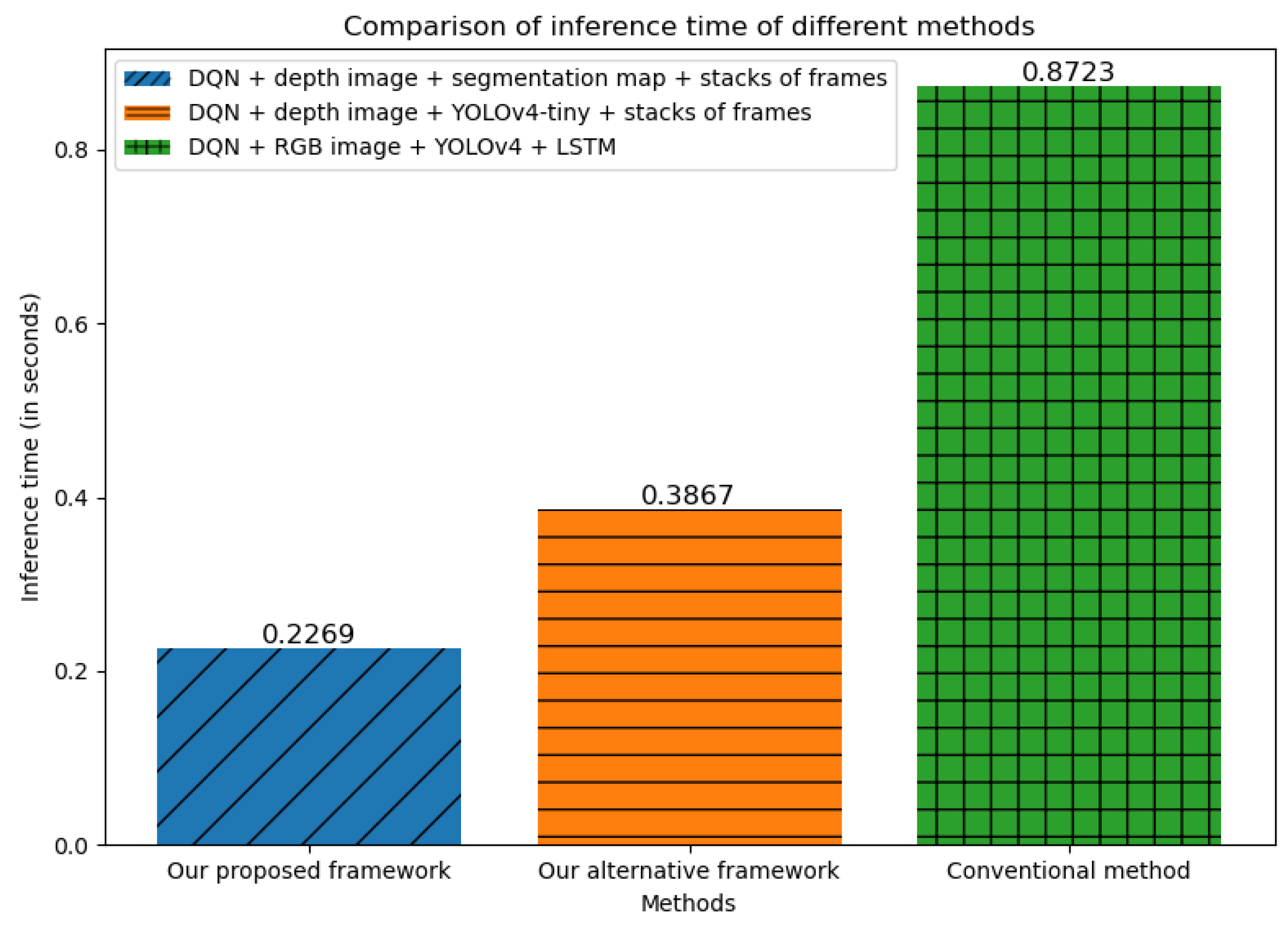The comparison between the processing time of depth images and RGB images using our framework is presented in Section 5. In addition, for the UAVs to be able to track objects effectively, they need to retrieve the objects’ historical movements. The possible candidates to capture sequential data are RNN, LSTM, and GRU. However, those networks would add much more computational costs. We decide to eliminate the need of sequence models and use a stack of consecutive frames to achieve the same goal but with much fewer computations (approx. a 50% reduction in the inference time, as shown in Figure 1).

In this paper, we propose a LDVRL framework to minimize the computational resources for UAVs to perform dynamic object tracking, which consists of:

• A segmentation map method to extract the object boundaries. This method can run in $O\left(1\right)$ time complexity in the simulation tool. For UAVs to operate in the real world in future work, we implement the YOLOv4-tiny model to detect objects.
• We eliminate the computational cost of sequence models such as RNN, LSTM, and GRU by using stacks of consecutive frames.
• We construct our state space to use depth images instead of RGB images, not only to reduce computational resources but also to improve the obstacle avoidance ability.

The two DRL algorithms implemented in our experiment are DQN and DDPG. They are implemented under the same LDVRL system that we propose in Section 4. This paper introduces not only the LDVRL approach but also significant insights and comparisons between DQN and DDPG performance in the dynamic object-tracking task. Our finding shows that the LDVRL is capable of adapting to different DRL algorithms and a more complex algorithm is not necessary to be more efficient in every task. The comparison between our methods and the ordinary methods is given in Section 5.

2. Related Work

Various attempts have been made to solve the object tracking problem using traditional decision-making systems, such as the Visual Simultaneous Localization and Mapping (VSLAM) method [10]. However, the VSLAM method is limited in generalization because it is based on a pre-set model. In real life, modeling complex environments with dynamic and stochastic scenes is a challenging procedure. Furthermore, the method lacks robustness due to the accumulation of sensor noises that propagate from mapping, and localization to path planning. Another prominent issue is that VSLAM requires case-specific and scenario-driven engineering, which limits the practical application of VSLAM.

An alternative approach is to employ Reinforcement Learning (RL) techniques. RL allows agents to learn and act in complex and dynamic environments. By taking action and receiving the corresponding rewards, agents can learn and behave effectively to earn the highest rewards from the environment. Q-learning [11] is the most popular algorithm in this category. However, owing to the constraint of using a Q-table, this algorithm needs to know all states in the environment beforehand to initialize the Q-value table. As a result, tabular-based RL algorithms are not suitable for high-dimensional and continuous state space problems. Since the real world is a constantly changing environment with an infinite number of states, the original RL approaches cannot be applied well in that scenario.

The Deep Q-network (DQN) [12] improved upon RL via an ingenious fusion of Deep Learning (DL) and RL. It combines the generalization capabilities of DL with the decision-making capabilities of RL. Although a DQN has been investigated in simulation environments for autonomous navigation or target tracking [13,14], the majority of it depends on numerous additional tools which makes it very large in size and cannot be transferred efficiently to the UAVs with limited computing resources.

Policy gradient [15] and Actor-critic [16] methods emerged as another group of RL algorithms which have the ability to work in continuous action space. In [17], Zhaowei et al. use the actor-critic approach combined with a RBF neural network to implement the UAV’s obstacle avoidance. The result was not very remarkable since the parameter selection needs further improvements. Zhu et al. [18] propose a target-driven visual navigation system for indoor robots using an actor-critic model. Their approach shows the generalization ability across unseen indoor scenes and targets, and also improves the data collection efficiency. A Deep Deterministic Policy Gradient (DDPG) [19] is a DRL algorithm that incorporates a DQN with an actor-critic mechanism, which enables the operations in both continuous state and action spaces.

In order to track a dynamic object successfully, using only the DRL algorithm is not sufficient, and we need a good mechanism to detect objects as well. In [20], the authors develop a method that adopts YOLOv5 to detect unauthorized UAV incursions. In [21], the YOLOv5 backbone is replaced with Efficientlite to reduce the number of parameters in the model. The performance is also improved by injecting spatial feature fusion. The authors achieved better detection performance than YOLOv5 solely. While these papers focus on detecting UAVs only, the authors of  [22] apply an improved version of YOLOv4 on UAVs to detect different types of objects. They use hollow convolution, ULSAM mechanism, and soft non-maximum suppression to achieve a 5% improvement on the original YOLOv4 algorithm. Wentong et al. [23] achieved an advancement in small object detection using a local FCN with YOLOv5. However, no experiment has been conducted to directly study the usage of YOLO models in dynamic object tracking for UAVs to the best of our knowledge. Additionally, we are not only aiming to solve the detection problem in object tracking tasks individually but also trying to find the most lightweight approach in order to make it applicable to physical UAVs.

In our experiment, to reduce the size of DRL systems and make them feasible for applying on physical UAVs (to be under 1GB, as specified in Section 3.2), we use depth images as the only input source for decision making because they not only give a better sense of the surrounding obstacles but also have a smaller size than RGB images. RGB images have three channels (Red, Green, Blue) while depth images (greyscale) have only one channel; thus, reducing the size of depth images to one-third of the RGB images size. The simulation library we use AirSim [24] (described in Section 4.1) provides several APIs for accessing the depth images generated by the simulation (https://github.com/microsoft/AirSim/blob/main/docs/image_apis.md, accessed on 15 November 2022). In addition, to give the UAV better predictions of the target’s movements, we pile a number of consecutive depth frames to create a short video that captures the historical movements of the target. Initially, we intended to use Long Short-Term Memory (LSTM) [25] to process the sequential movements. However, we realize that adding a LSTM will generate an unnecessary overhead cost to the computational resources of the UAV. Therefore, we elegantly switch to use a short video of depth images to accomplish the same goal, but with much lower computations. In the simulation environment, we use a segmentation map to localize the target object in the current frame because it is extremely lightweight and convenient, and some UAVs nowadays already offer the integration of a segmentation camera such as the DJI Phantom 4 RTK, DJI Matrice 300 RTK, Intel Falcon 8+, Parrot Anafi USA, etc. For UAVs that do not have segmentation cameras, we adopt the current lightest object detection model (YOLOv4-tiny) to detect the objects. Furthermore, we design an effective non-sparse reward function to help the UAV to learn and track the target effectively. In this paper, we test our LDVRL system with both DQN and DDPG algorithms to see the adaptability of our framework and, finally, compare their performance under the same settings. Since a DDPG is an extension of a DQN, it is expected to give a better performance. However, a DQN shows better metrics for this task surprisingly. The details are discussed in Section 5.

3. Preliminaries

3.1. Problem Statement

The goal of this experiment is to fly an UAV to autonomously follow a designated target object over a specified duration, while simultaneously avoiding collisions with any surrounding obstacles. The target object exhibits dynamic behavior, possessing the ability to move in arbitrary directions during the mission. The UAV’s operations are performed under the constraints of continuous state space (which represents the range of possible positions and orientations) and discrete action space (a finite set of possible control commands). A notable aspect of this experiment is the exclusive reliance on depth images as the primary source of input data for the UAV’s navigation and tracking functions. These images are captured by a front-mounted camera, providing crucial information on the relative position and distance of the target object and any potential obstacles in the UAV’s flight path. The UAV’s state observations rely entirely on the camera inputs, effectively eliminating the need for additional tools or equipment such as sensors or GPS.

3.2. Scope and Constraints

The scope of this research project is primarily focused on developing a lightweight DRL-based method for tracking target objects using multirotor UAVs, which possess the ability to hover in place [26]. Other UAV types that do not support vertical take-off and landing (VTOL) or hovering are not considered in this paper.

During the development and testing phases, the method was implemented and evaluated within a simulation environment. The simulation environment gives us immediate access to critical data, including segmentation maps and depth images. The use of a simulated environment also helps to minimize potential risks during the development process.

However, this project is constrained by the fact that real-world testing has not been conducted within its current scope. The primary focus has been on the development and evaluation of the proposed method in a simulated environment, and the transition to real-world testing presents a range of additional challenges that may impact the system’s performance. These challenges may include factors such as variations in lighting, environmental conditions, and potential discrepancies between the simulated and real-world data. We try to extend the project’s scope in the future to encompass real-world testing of the developed method. This expansion would provide valuable insights into the algorithm’s robustness and adaptability in practical settings, further validating the effectiveness of the DRL approach for UAV tracking tasks.

The minimum resource requirements that can be suitable for running the proposed method on UAVs are (these requirements are equivalent to the resources on the simulated UAVs used in our experiments):

• Onboard processor: a low-power, energy-efficient processor with a minimum of two cores, such as the ARM Cortex-A series (e.g., Cortex-A53 or Cortex-A72), to handle real-time data processing and decision making during the operation.
• Onboard memory (RAM): a minimum of 2 GB of RAM to store the DRL model (approx. 1 GB), manage input data processing, and facilitate real-time decision-making.
• Storage: sufficient onboard storage capacity (e.g., 8 GB or larger) to accommodate the DRL model, input data buffers, and other essential software components.
• Camera system: a depth-sensing camera system compatible with the UAV’s processor and capable of providing the required depth images for the DRL method. The segmentation camera is only needed when we want to utilize the best-proposed method. Otherwise, we employ a YOLOv4-tiny in our alternative proposed method for UAVs that are not equipped with a segmentation camera.
• Software environment: compatibility with the required software libraries and frameworks for running the DRL model on the onboard processor (e.g., TensorFlow Lite, PyTorch Mobile).

3.3. Reinforcement Learning

Almost every RL problem is modeled as a Markov Decision Process (MDP). A MDP [27] is a powerful framework for modeling decision-making problems in which the outcomes are unpredictable. The MDP is driven by a tuple of $(S,A,P,R,\gamma )$, where $S=\{s_1,s_2,\dots ,s_n\}$ is the set of states (state space) and each state is a representation of an environment observation, $A=\{a_1,a_2,\dots ,a_n\}$ is the set of actions (action space), $P(s^{\prime }\mid s,a)=P[S_{t+1}=s^{\prime }\mid S_t=s,A_t=a]$ is the state transition function which indicates the probability of getting state $s^{\prime }$ and reward r when taking action a in state s, $R(a,s)=\mathbb{E}[R_t\mid S_t=s,A_t=a]$ is the reward function, and $\gamma \in [0,1]$ 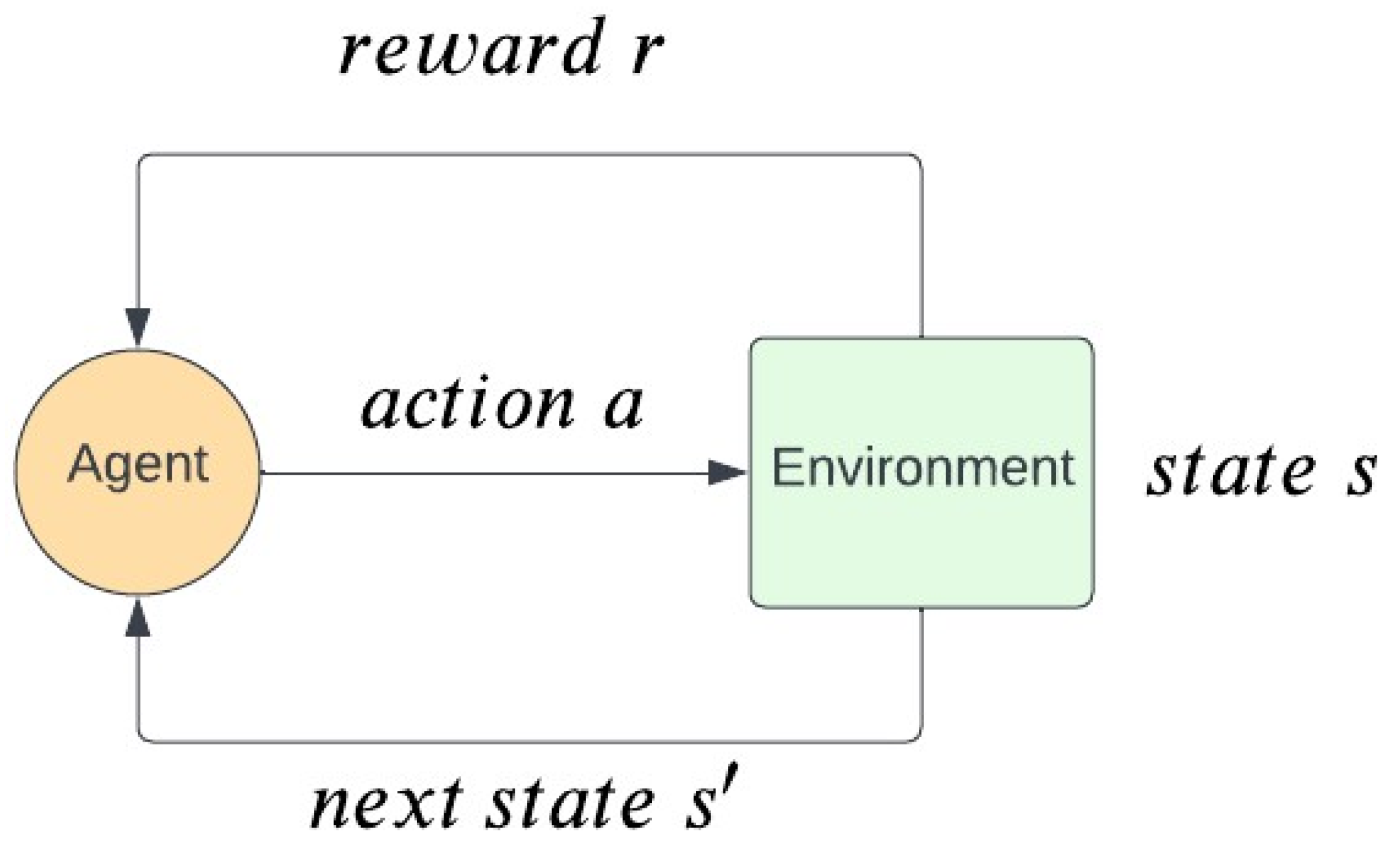is the discount factor, which helps to converge the infinite sum of rewards in continuing tasks. The agent takes actions in accordance with its policy $\pi (a\mid s)=P[A_t=a\mid S_t=s]$. A policy is a mathematical function that receives a state and returns the probabilities of taking each action in the action space. A policy can be either deterministic or stochastic. The aim of a policy is to maximize the expected discount return $G_t=\mathbb{E}\left[{\sum }_{t=0}^{\infty }{\gamma }^{t}R(S_t,A_t)\right]$, where $A_t$ is sampled from the policy $\pi (A_t\mid S_t)$. The MDP framework can be visualised in Figure 2.

The object-tracking task can be modeled as an MDP where the objective is to find the optimal policy that can produce optimal actions according to the current state. The interaction between the UAV and the environment is defined by the reward function and state transition function.

3.4. Q-Learning

Q-learning is a model-free, off-policy, and value-based RL method that uses the Bellman Equation (1) to update its value function.

$$V\left(s\right)=ma{x}_a\left[R(s,a)+\gamma V\left(s^{\prime }\right)\right]$$

(1)

where $V\left(s\right)$ is the value of state s, $R(s,a)$ is the reward of taking action a in state s, $\gamma$ is the discount factor, and $V\left(s^{\prime }\right)$ is the value of the next state.

The main idea behind Q-learning is to store a table of Q-values for all state-action pairs that reflect how beneficial to take an action at a particular state. A Q-value is expressed as $Q(s,a)={\mathbb{E}}_{\pi }\left[R_t\mid s_t=s,a_t=a\right]$. Using the TD learning approach, Q-values are updated using the following equation:

$$Q(s,a)=Q(s,a)+\alpha \left[R(s,a)+\gamma \underset{a^{\prime }}{\mathit{max}}Q(s^{\prime },a^{\prime })-Q(s,a)\right]$$

(2)

where $Q(s,a)$ is the Q-value of taking action a at state s, $\alpha$ is the learning rate, $R(s,a)$ is the reward of taking that action, $\gamma$ is the discount factor, and $Q(s^{\prime },a^{\prime })$ is the Q-value of taking action $a^{\prime }$ at state $s^{\prime }$.

In the beginning, the Q-table is initialized with all zeros by default. We can achieve better optimization if we initialize the Q-table with values higher than the upper bound of all state-action values because it encourages the agent to explore state-action pairs that are not yet visited. During the learning process, the agent explores different state-action pairs and updates the Q-value table using Equation (2). In the end, an optimal policy is obtained by choosing the most beneficial action in every state.

3.5. Actor-Critic Methods

From Section 3.3, we have seen that the goal of any RL algorithm is to find the optimal policy that produces the highest return. This goal can be achieved by either a policy-based algorithm or a value-based algorithm. In value-based RL (e.g., Q-learning), the optimal policy is derived implicitly by calculating the optimal value function. The most profitable action at each state (according to the value function) is selected to generate the policy afterward. On the other hand, policy-based RL algorithms directly compute the optimal policy. While policy-based RL is effective in high dimensional and stochastic continuous action spaces, value-based RL has advantages in sample efficiency and stability. Actor-Critic methods are Temporal Difference (TD) methods that utilize both policy-based and value-based RL. It has an actor network, which is a policy-based component and is responsible for choosing actions at a given state. It also has a critic network, which is a value-based component that evaluates the actions selected by the actor. The critic uses a TD error to assess whether the actor has selected a good action via the following equation:

$$\delta =r+\gamma V\left(s^{\prime }\right)-V\left(s\right)$$

(3)

where $\delta$ is the TD error, V is the value function calculated by the critic, s is the current state, $s^{\prime }$ is the next state, r is the reward, and $\gamma$ is the discount factor. If this TD error is positive, it means the action a should be selected more often. Otherwise, it means action a should be selected less often. Using actor-critic methods, we have the following benefits:

• It can work in infinite and continuous action space.
• Stochastic policy is learned explicitly. This ability is very useful in non-Markov cases (for example, in [28]).

4. Research Methodology

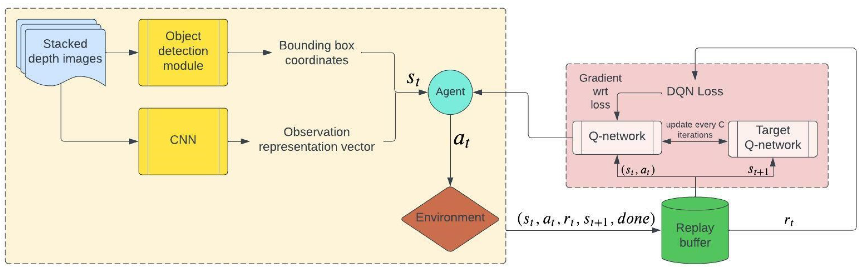
In this section, we explain in detail about our methodology. We use Figure 3 to illustrate the components of our proposed method and provide an overview of our system. The detail of each component is discussed in the subsections below. The algorithm’s detail can be viewed in Algorithms 1 and 2.

Algorithm 1 Deep Q-Network

Algorithm 2 Deep Deterministic Policy Gradient

4.1. Simulation Environment

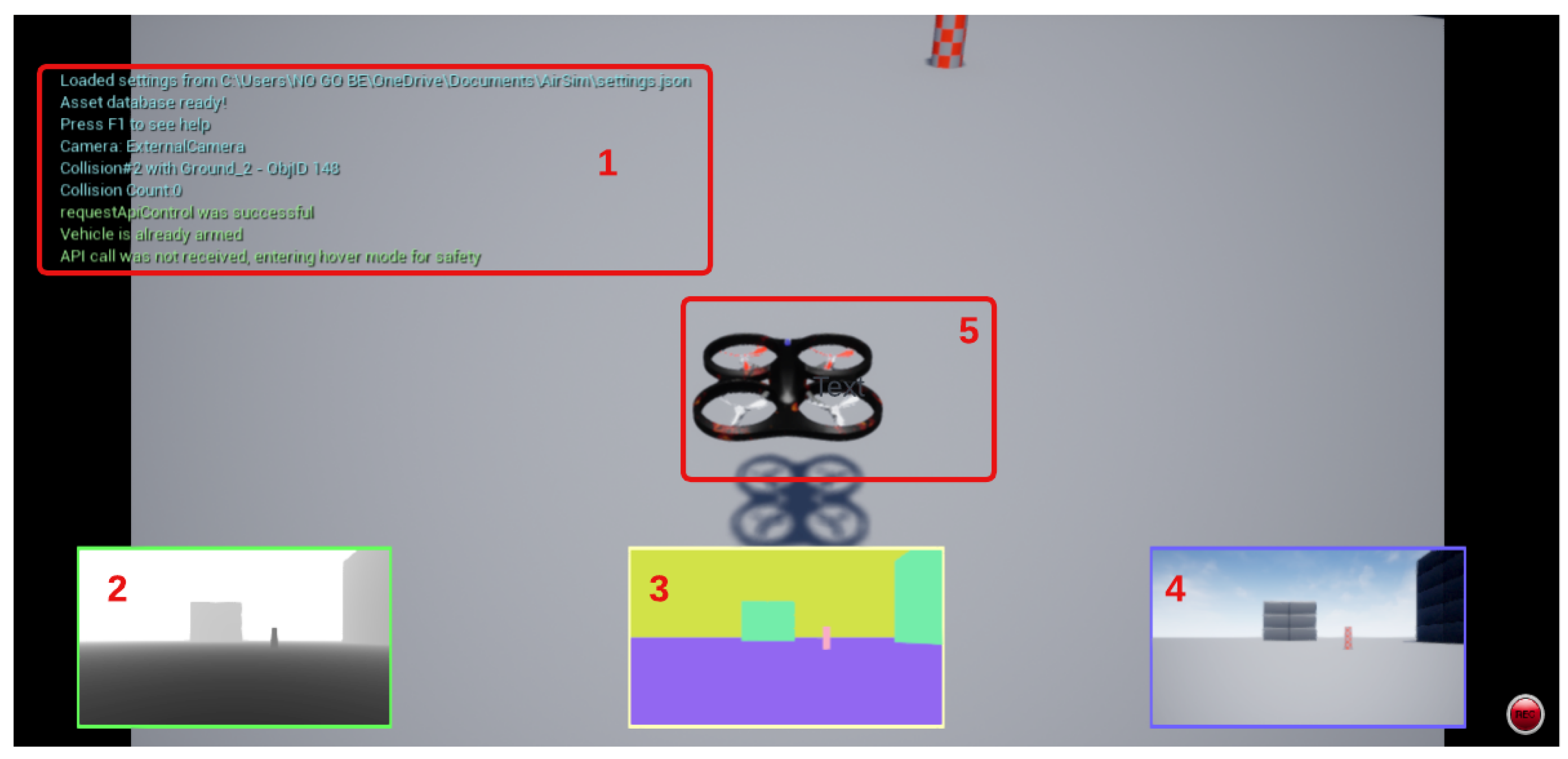
Training a physical UAV in the real world is expensive since it involves a repeated process of trial and error, which can result in severe damage to the UAV or objects around it. Thus, a simulation environment is acquired. We choose Airsim [24] because it is a powerful plugin that works inside the Unreal Engine, which allows us to use numerous high-fidelity pre-built 3D environments to train our agent. Airsim can generate a quadcopter that is equipped with three different cameras: RGB, depth, and segmentation (Figure 4). In our method, we need to work with both depth and segmentation images. The other advantage of using Airsim is that it establishes easy connectivity with PixHaw API, which makes our implementation very quick to be transferred onto a physical UAV.

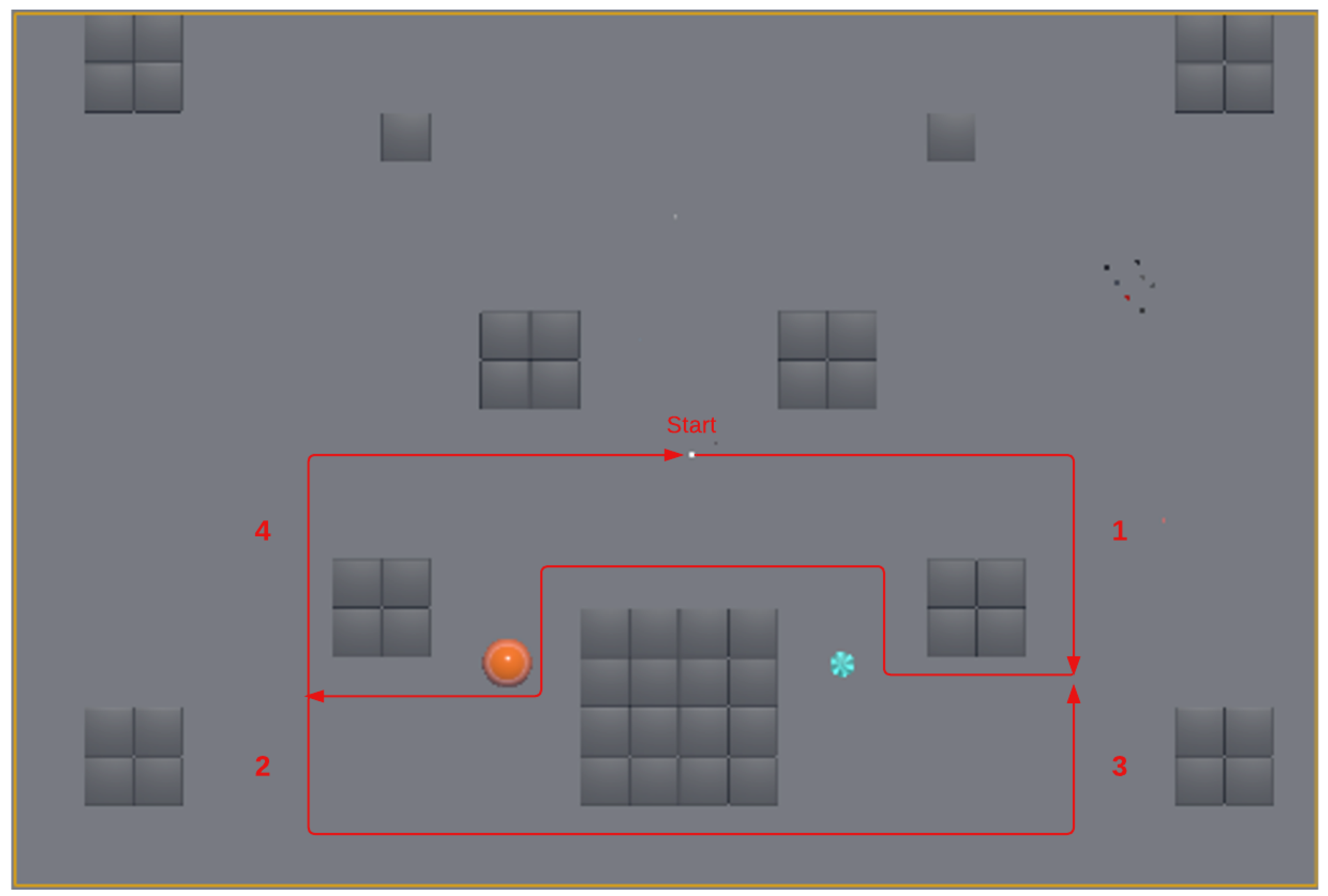
We design an 11,500 m${}^2$ rectangle area with random obstacles scattered around. Our target object can move freely in the environment. The path of the target object is predefined and shown in Figure 5. To avoid bias toward certain behaviors, we keep the number of right turns and left turns balanced (eight right turns, eight left turns). There is only at most one target object moving in the environment at a time. We place obstacles with different sizes and shapes to allow the agent to learn different situations.

4.2. Deep Q-Network (DQN)

The issue with Q-Learning is that we have to determine Q-values for all state-action pairs in the environment. This is only possible when the state space is discrete because the continuous state space has an infinite number of states, and it is impossible to determine the Q-value for all of them. However, the state representation used in our experiment is continuous (e.g., a sequence of images) which makes the mapping of every state to a Q-value impractical. Therefore, instead of storing a Q-values table, we approximate the Q-values using neural networks. The input of a network is the state observation, and the output of the network is the approximated Q-value for all possible actions at that state. We trade the accuracy of the Q-table for the generalization ability of the neural networks. A DQN has two important techniques that help to reduce training instability: Experience Replay and Target Network.

Originally proposed in [29], Experience Replay is used to prevent the over-fitting issue of deep neural networks. It stores the state, action, reward, and next state of some latest steps. Experience Replay is used for sampling batches when training the DQN. With this mechanism, Experience Replay can reduce the correlation between experiences and improve the training speed by using mini-batches.

For the “Target Network” technique, we can see from Equation (2) that the predicted value $Q(S_t,A_t)$ and the target value $\left[R_{t+1}+\gamma {\max }_{a}Q(S_{t+1},a)\right]$ are not independent because they both use the same network. Therefore, instead of using one neural network for learning, we can use a Q-network and Target Q-network separately. Using two networks results in improved stability and efficiency of the learning process.

The implementation detail of this algorithm in our approach can be viewed in Algorithm 1. Firstly, we initialize the essential objects, which are the Airsim UAV, the target’s segmentation ID, the Environment, the Q-network, the Target Q-network, the Experience Replay, and the DQN agent. The second step is to collect sample experiences for the Experience Replay. We initialize a random policy that selects a $ϵ$-greedy action to fill the Experience Replay partially. Then, the DQN is ready to be trained. For a certain number of epochs (we use 400 epochs in our experiment), repeat the following actions:

• Perform actions according to the current policy and store the transition into the Experience Replay.
• Sample a random training batch from the Experience Replay. For each element in the batch, we pass the current state through the Q-network to get the Predicted Q-value. The next state is used as an input to the Target Network and we only keep the maximum of the returned Q-values. This highest Q-value is then added with the immediate reward to compute the Target Q-value.
• Compute the Mean Squared Error Loss between the Predicted Q-value and the Target Q-value.
• Backpropagate the loss and update the Q-network.
• After every M steps, copy the weights from the Q-network to the Target Q-network.

4.3. Convolutional Neural Network (CNN)

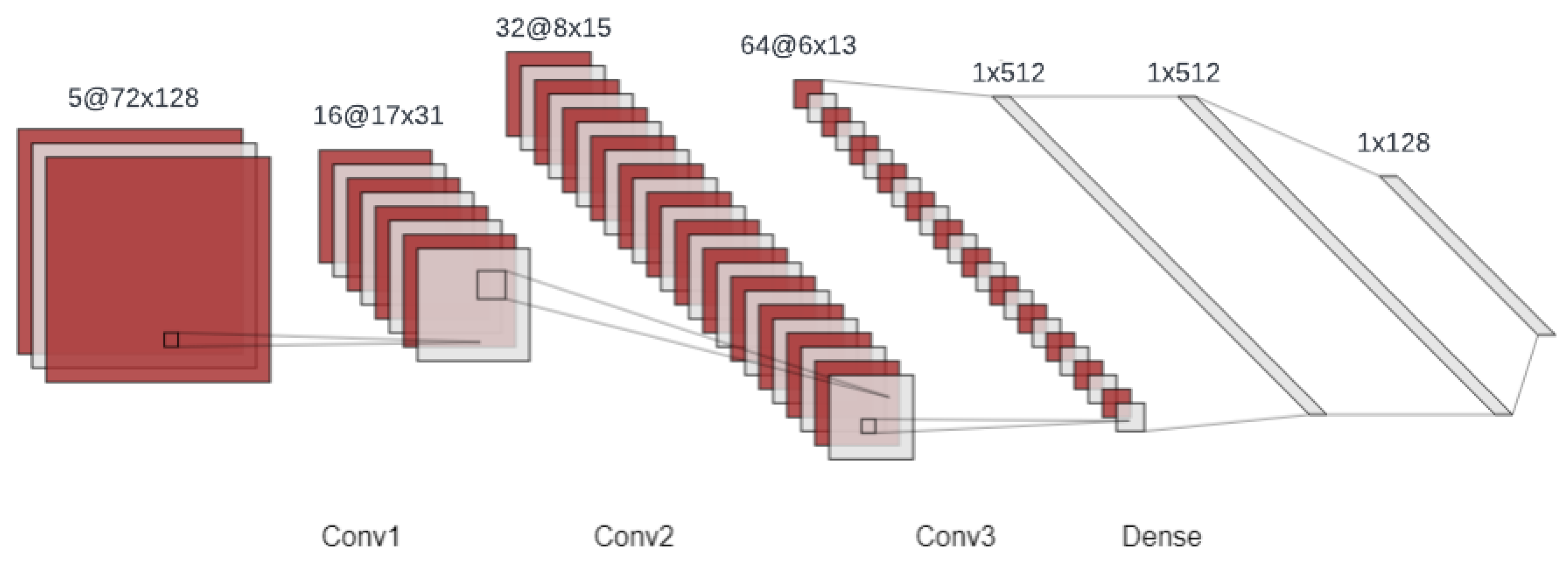
Since the input source of our LDVRL system is images, we adopt a CNN [30] to process and extract the important features of the images before passing them into our DRL agent. In our system, the observations at each state (five consecutive depth frames, as described in Section 4.6) are passed into the CNN to extract the features. We use three layers of convolution. The first layer contains 16 kernels of 5 × 5, and the stride is 4. The second layer has 32 kernels of 3 × 3, and the stride is 2. The last layer uses 64 kernels of 3 × 3, and the stride is 1. Then, a fully connected network of 3 layers is used to extract the final representations of the input before passing them to the DQN to approximate the value for each possible action at that state. After the value function is trained, inferring the optimal policy is straightforward. The agent only needs to exploit the most profitable action at each state. The illustration of our CNN architecture can be seen in Figure 6.

Figure 6 illustrates the architecture of the CNN used in our DRL algorithms. The input to the CNN is five consecutive depth frames, which serve as our state representation. Each frame has a resolution of 72 × 128 pixels, as this is the image resolution returned by AirSim APIs, as explained in detail in Section 4.6. The input is then fed into three convolutional layers that detect relevant patterns in the frames. The output of these convolutional layers is then flattened and passed through three dense layers that further process the information. Finally, the output is condensed into a 1 × 128 vector that represents the state of the system at that particular time step. This vector is then used as an input to the DRL algorithms, together with the bounding box coordinates, as shown in Figure 7, to make decisions about the UAV’s actions.

4.4. Deep Deterministic Policy Gradient (DDPG)

A DDPG is a typical example of the Actor-Critic method. It has two distinct networks: the Actor (denoted by $\mu$), and the Critic (denoted by Q). In order to improve the stability of the learning, two more target networks are used: one is for the Actor, and the other is for the Critic. Therefore, the DDPG algorithm has four networks: one Actor, one Critic, one Target Actor, and one Target Critic. The target networks are updated via soft update. The role of the Actor is to decide which action is the best to pick based on the current state. On the other hand, the Critic evaluates state and action pairs, giving the Actor feedback on whether the taken actions are good in that state. The DDPG uses a deterministic policy, which produces the action values, but not the probabilities. The deterministic policy has a problem with the explore-exploit dilemma. This issue can be reduced by adding some extra noise into the output of the Actor Network (e.g., the Gaussian noise). The update rule of the Actor Network is:

$$\begin{array}{c}\hfill {\nabla }_{{\theta }^{\mu }}J\approx {\mathbb{E}}_{S_t\sim {\rho }^{\beta }}[{\nabla }_{{\theta }^{\mu }}Q\left(s,a\mid {\theta }^Q\right)\mid \\ \hfill s=S_t,a=\mu \left(S_t\mid {\theta }^{\mu }\right)]\end{array}$$

(4)

where ${\theta }^{\mu }$ is the parameter of the Actor Network $\mu$, ${\theta }^Q$ is the parameter of the Critic Network Q, $\mu (S_t\mid {\theta }^{\mu })$ is the action chosen by the Actor Network $\mu$ at state $S_t$, and $Q(s,a\mid {\theta }^Q)$ is the state-action value when taking action a in state s. The objective of the Critic Network is to shift the estimated state-action value $Q(s,a)$ as close as possible to the target value. The target value is defined as:

$$y_i=r_i+\gamma Q^{\prime }(S_{i+1},{\mu }^{\prime }(S_{i+1}\mid {\theta }^{{\mu }^{\prime }})\mid {\theta }^{Q^{\prime }})$$

(5)

where $r_i$ is the current reward, $S_{i+1}$ is the next state, $Q^{\prime }(·)$ is the state-action value estimated by the target Critic Network, and ${\mu }^{\prime }(·)$ is the action chosen by the target Actor Network. The objective of the Critic Network can be achieved by minimizing the following loss function:

$$L=\frac{1}{N}\sum _i{\left(y_i-Q\left(S_i,A_i\mid {\theta }^Q\right)\right)}^2$$

(6)

where $y_i$ is the target value defined in Equation (5).

At the beginning, the weights ${\theta }^{\mu }$ and ${\theta }^Q$ of the Actor Network $\mu (s\mid {\theta }^{\mu })$ and the Critic Network $Q(s,a\mid {\theta }^Q)$ are randomly initialized. After that, those parameters are copied exactly into the corresponding target network, and this is the only time the exact hard copy is executed. Since then, the “soft update” rule has been adopted and it only makes partial updates from the original networks. The soft update rule is described below:

$$\begin{array}{c}{\theta }^{{\mu }^{\prime }}\leftarrow \tau {\theta }^{\mu }+(1-\tau ){\theta }^{{\mu }^{\prime }}\\ {\theta }^{Q^{\prime }}\leftarrow \tau {\theta }^Q+(1-\tau ){\theta }^{Q^{\prime }}\end{array}$$

(7)

where ${\theta }^{{\mu }^{\prime }}$ is the weights of the target Actor Network, ${\theta }^{Q^{\prime }}$ is the weights of the target Critic Network, and $\tau$ is a small number that is close to 1 (e.g., 0.99).

The implementation detail of this algorithm in our approach can be viewed in Algorithm 2. Similar to the DQN, we need to initialize the essential objects in the first step, which includes the Airsim UAV, the target object’s segmentation ID, the Environment, the Experience Replay, the Actor Network, the Critic Network, the Target Actor Network, the Target Critic Network, and the DDPG agent. Then, we initialize a random policy that selects the $ϵ$-greedy action to fill the Experience Replay partially. After that, the DDPG agent can use the data in the Experience Replay to train. For a certain number of epochs, we repeat the following actions:

• Choose the action according to the current Actor Network.
• Add clipped noise to the chosen action to balance the explore-exploit dilemma. Perform the action, observe the transition, and store it in the Experience Replay.
• Sample a random training batch from the Experience Replay. For each element in the batch, we pass the next state to the Actor Network to get the next action. That (state, action) pair is fed into the Critic Network to get the next Q-value, which is get multiplied by the discount factor and added with the immediate reward to compute the Target Q-value. The Predicted Q-value is calculated by passing the current state and the current action into the Critic Network.
• After that, we determine the Mean Squared Error Loss between the Target Q-value and the Predicted Q-value.
• We backpropagate the loss to update the Critic Network.
• The Actor Network is updated using the Policy Gradient formula.
• The Target Actor Network and Target Critic Network are updated using a soft update.

4.5. Action Space

A DQN is designed around discrete action spaces—the set of actions we use for moving the UAVs comprises eight actions: MoveRight, MoveLeft, TurnRight, TurnLeft, MoveUp, MoveDown, MoveForward, and Hover. If an action is chosen, a fixed velocity and duration is applied to move the UAV in that chosen direction. Each action is represented as an integer between 0 and 7, as illustrated in

Table 1. Mapping from the DRL algorithm’s output to actions.

Interger	Action
0	MoveRight
1	MoveLeft
2	TurnRight
3	TurnLeft
4	MoveUp
5	MoveDown
6	MoveForward
7	Hover

. This set of actions is chosen because it enables the flexibility of the UAV to fly in any direction. The moving backward action is omitted because the UAV cannot see what is behind; thus, making a backward action is dangerous. When running the experiment with a DDPG, although the algorithm can deal with continuous actions, we still use this set of discrete actions to keep it as a fair competition with a DQN. We can only compare the performance between them if all the settings are the same.

4.6. State Space

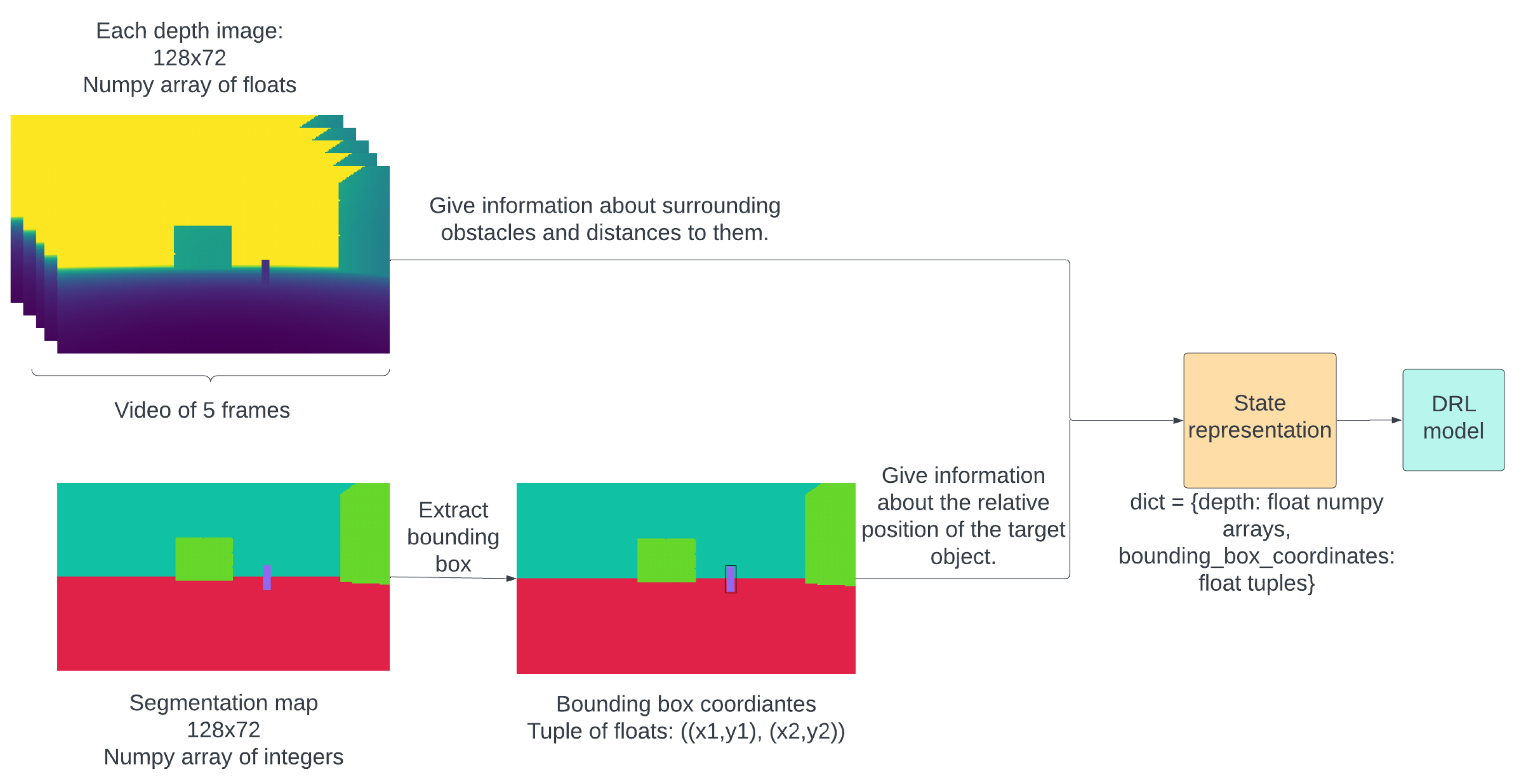
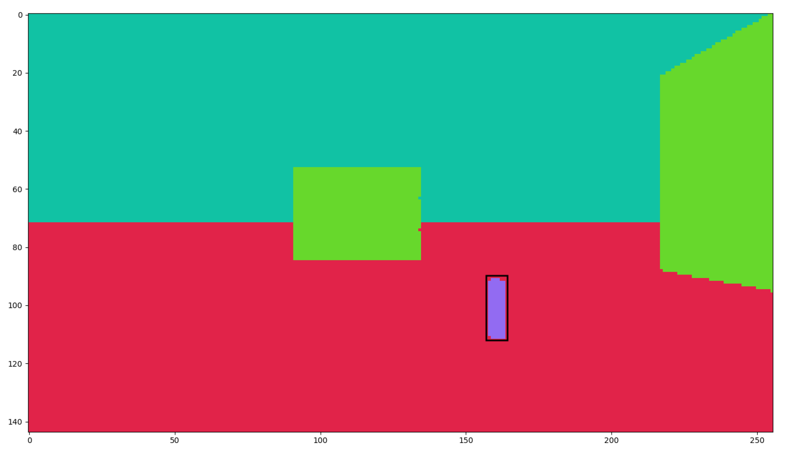
State representation allows the agent to identify different situations and make decisions based on the environment. To create a complete observation, the UAV’s front-mounted camera processes the segmentation map, outputting the target object’s bounding box coordinates. These coordinates are then combined with a short video consisting of five consecutive depth map images from the same camera view, each delayed by 0.1 s.

Depth map images are acquired directly from AirSim using its APIs (https://microsoft.github.io/AirSim/api_docs/html/, accessed on 15 November 2022). Depth map images provide information about obstacles in the environment. They are more efficient than RGB images, as they contain distance information and they use a single channel, reducing the size to one-third compared to RGBs. The agent utilizes bounding box coordinates to identify the target object and depth map images to navigate around obstacles.

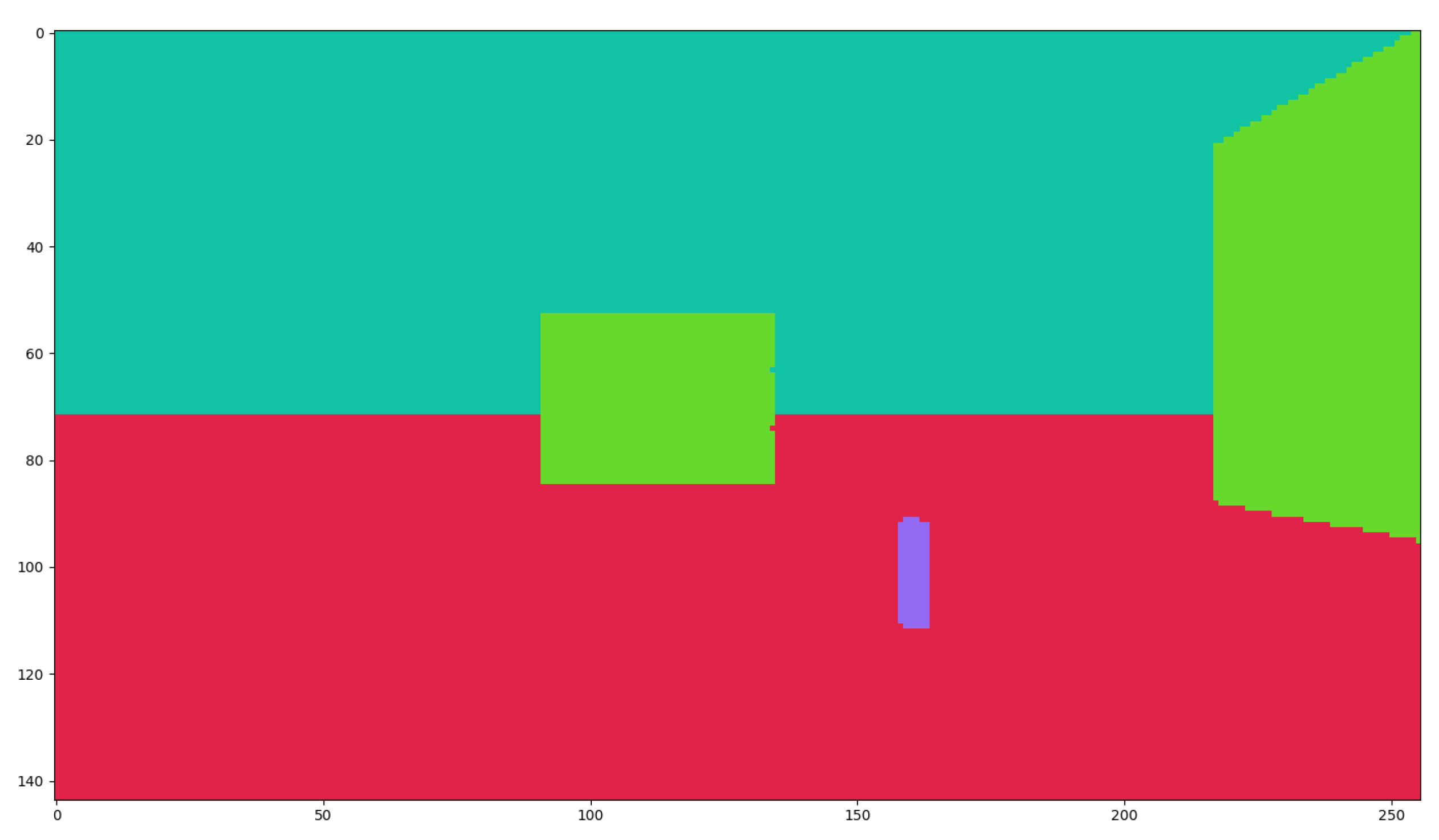
A segmentation map is also acquired from AirSim APIs (https://microsoft.github.io/AirSim/api_docs/html/, accessed on 15 November 2022). During the initial setup, a specific RGB value is assigned to the target object in the segmentation map, which has the same camera view as the depth images. This assignment enables easy identification of the target object and accurate extraction of the bounding box. All images returned by AirSim’s APIs (https://microsoft.github.io/AirSim/api_docs/html/, accessed on 15 November 2022) have a resolution of 128 × 72. Examples of a segmentation map and a complete state representation can be seen in Figure A1 and Figure 7, respectively.

4.7. Reward Function

The reward function is crucial for the learning process; a good reward function is able to balance exploration and exploitation. In our approach, we neither make the reward function too specific nor too simple. This reward function allows effective learning while maintaining exploration. Firstly, we extract the bounding box coordinates from our object detection module because it holds two useful pieces of information: the distance from the UAV to the target, and the relative position of the target. There are two types of rewards in our reward function design: positive and negative. Positive rewards are given when the bounding box lies entirely within the middle 50% of the image width. We chose 50% because after trying with different thresholds, 50% showed the most satisfying results, as shown in

Table 2. Experiment with different thresholds for positive reward.

Image Width	Average Episode Length (Steps)
25%	21.25
30%	24.73
35%	25.32
40%	28.91
45%	27.28
50%	34.50
55%	32.13
60%	28.91

. Because all images are 128 × 72 pixels, we can tell the bounding box is inside the middle 50% if the top-left x-coordinate of the bounding box is greater than $128·\frac{1}{4}=32$ and its bottom-right x-coordinate is less than $128·\frac{3}{4}=96$. The amount of this positive reward is defined as the distance between the bounding box center and the frame center. The closer the distance is, the higher reward the UAV can achieve. That is because we want to encourage the UAV to keep the target as close to the center as possible.

The agent gets negative rewards (penalties) when the bounding box is within the left 25% or the right 25% of the image width, as the middle 50% is allocated for positive rewards. This penalty discourages the agent from keeping the target object in the left or right 25% of the image width because there is a high probability that the target will move out of the current view from those regions. The agent also gets penalties when it makes a collision with an object. Furthermore, to prevent the agent from approaching too close to the target, we also apply a penalty if the bounding box height occupies more than 50% of the image height. On the other hand, to prevent the agent from positioning too far away from the target, the penalty is also applied if the bounding box height takes less than 10% of the image height. Because all images are 128 × 72 pixels, 50% of its height equivalents to $\frac{72}{2}=36$ pixels and 10% of its height is equivalent to $\frac{72}{10}=7.2$ pixels. We choose these thresholds as a baseline to run our experiment. Other thresholds and their performances will be investigated further in future works. Our complete reward function is defined as:

$$reward=\left\{\begin{array}{cc}-1\hfill & \mathrm{if}\mathrm{collides}\hfill \\ \frac{1}{distance}\hfill & \mathrm{if}{x}_1>32\mathrm{and}{x}_2<96\hfill \\ -distance\hfill & \mathrm{if}{x}_1\le 32\mathrm{or}{x}_2\ge 96\hfill \\ -\frac{boundingBoxHeight}{imageHeight}\hfill & \mathrm{if}boundingBoxHeight>36\mathrm{pixels}\hfill \\ -\frac{0.1·imageHeight}{boundingBoxHeight}\hfill & \mathrm{if}boundingBoxHeight<7.2\mathrm{pixels}\hfill \\ 0\hfill & \mathrm{otherwise}\hfill \end{array}\right.$$

(8)

where $distance$ is the Euclidean Distance between the bounding box center and the frame center, $x_1$ is the bounding box’s top-left x-coordinate, and $x_2$ is the bounding box’s bottom-right x-coordinate.

4.8. Training Configurations

Since both the DQN and DDPG sample batches from the Experience Replay, it is necessary to fill a portion of the Experience Replay before the training starts. We achieve this by performing random actions for 1000 steps. The current state, action, reward, and next state of each step are stored in the Experience Replay. The maximum size of our Experience Replay is set to be ten times bigger than the number of initial steps, which is 10,000 samples. This big number of samples can guarantee the DQN algorithm has sufficient experience to train our agent. Without this preparation, the training will collapse because there is no experience to be sampled during the training loop.

If the agent is able to hold the target in sight for 50 consecutive steps, the task is considered to be achieved. Therefore, we set the maximum number of steps in one episode to 100 to avoid wasting resources on useless experiences. If the agent has not learned properly, it always ends an episode within a couple of ten steps. If the agent is trained successfully, it only takes a maximum of 50 steps to finish the episode. We use the batch size of 64 and train the agent for 400 epochs. The training optimizer is Adam with a learning rate of 0.005.

The training phases of a DQN and DDPG are carried out separately from the operation of the UAV. During the training phase, the models are exposed to a variety of simulated scenarios in which they learn to generate optimal control commands for the UAV based on the depth images and segmentation map data. The primary reason for this separate training process is to ensure that the DRL methods are adequately trained and optimized before deployment in the tracking tasks. Once the DQN and DDPG have been trained and their performance has been validated in the simulated environment, the learned models can be deployed on the UAV’s onboard hardware during the operation phase. In this paper, our primary focus is on the training and validation aspects of the proposed algorithm, which provide the foundation for subsequent real-world deployment. The hardware we used to train the models is as follows:

• GPU: NVIDIA GeForce RTX 2060 (VRAM 6 GB GDDR6);
• CPU: Intel(R) Core(TM) i5-8400 CPU @2.80 GHz 2.81 GHz;
• RAM: 16 GB DDR4;
• Operating system: Windows 10, 64-bit;
• Storage: 1 TB HDD.

4.9. Dataset

DRL agents must be trained through extensive trial and error before they can acquire robust policies to complete tasks. In practical applications such as dynamic object tracking, creating training experiences can be particularly challenging, time consuming, and costly due to the unique properties of each environment. When training a DRL agent using an existing dataset, the environment and the features of the environment, such as the state transition function, should be the same in order to maximize the performance. As an alternative, we can allow the agent to learn from the experiences generated while interacting with our custom environment. We use Experience Replay (explained in Section 4.2), which is a crucial component of off-policy learning, to store those experiences. An experience stored in the Experience Replay consists of four elements $(s,a,r,s^{\prime })$, in which:

• State (s): this is the representation of the current state, before any action is taken by the agent.
• Action (a): the action the agent decides to take based on its policy $\pi$ and the current state s. This directly affects the next state $s^{\prime }$ and reward r.
• Reward (r): the reward returned from the environment for taking action a in state s.
• Next state ($s^{\prime }$): the results state that the agent gets in after taking action a in state s.

4.9.1. Data Collection

In our experiment, the capacity of the Experience Replay is set to be 10,000 entries. Those experiences allow the agent to learn from previous mistakes. Whenever the agent makes an interaction with the environment, it stores the transition in the Experience Replay for later use. Once the capacity limit is reached, old transitions are deleted to save new transitions. During the training phase, we sample a random batch from the Experience Replay to break the temporal correlation between the data and allow the agent to learn from a diverse set of experiences.

4.9.2. Data Description

Our Experience Replay contains 10,000 samples at most and they all have the same structure as a tuple of $(s,a,r,s^{\prime })$. The state and next state components are stored in Python Dictionaries with two keys: depth_frames and bounding_box, in which:

• Depth_frames: a numpy array of dimension 5 × 128 × 72 represents the values of five consecutive depth frames. Each frame has a resolution of 128 × 72 pixels and is retrieved directly from the simulation tool via AirSim APIs (https://github.com/microsoft/AirSim/blob/main/docs/image_apis.md, accessed on 15 November 2022).
• Bounding_box: a float tuple of $((x_1,y_1),(x_2,y_2))$ describes the top-left and bottom-right coordinates of the bounding box.

The reward component is a float (as described in Section 4.7), and the action component is an integer (as described in Section 4.5). The data description can be viewed in

Table 3. Data description of the parameters used in the DRL algorithms.

Component	Structure	Size
Experience Replay $\mathcal{D}$	Tuple of $(s,a,r,s^{\prime })$	10,000
State s & Next State $s^{\prime }$	Dictionary of {depth_frames: float numpy array, bounding_box: float tuple}	depth_frames: 5 × 128 × 73 bounding_box: $((x_1,y_1),(x_2,y_2))$
Reward r	Float	1
Action a	Integer	1

.

4.9.3. Data Annotation and Data Splits

Unlike Supervised Learning, RL does not need the training data to be annotated [31]. The agent should interact and learn directly from the responses of the environment. Additionally, the need for validation/test sets is also absent in RL. To evaluate the agent, we assess how the trained agent performs on the actual task and monitor the metrics introduced in Section 5. The Experience Replay we described in the above sections technically serves as a dataset in RL. However, compared to other paradigms (supervised and unsupervised), Experience Replay is not a traditional dataset, because of the following:

• The Experience Replay is not fixed; old experiences get deleted when the capacity is reached to store new experiences.
• It is not necessary to use every data point in the Experience Replay when training because the data are sampled in random batches from the Experience Replay.

5. Results

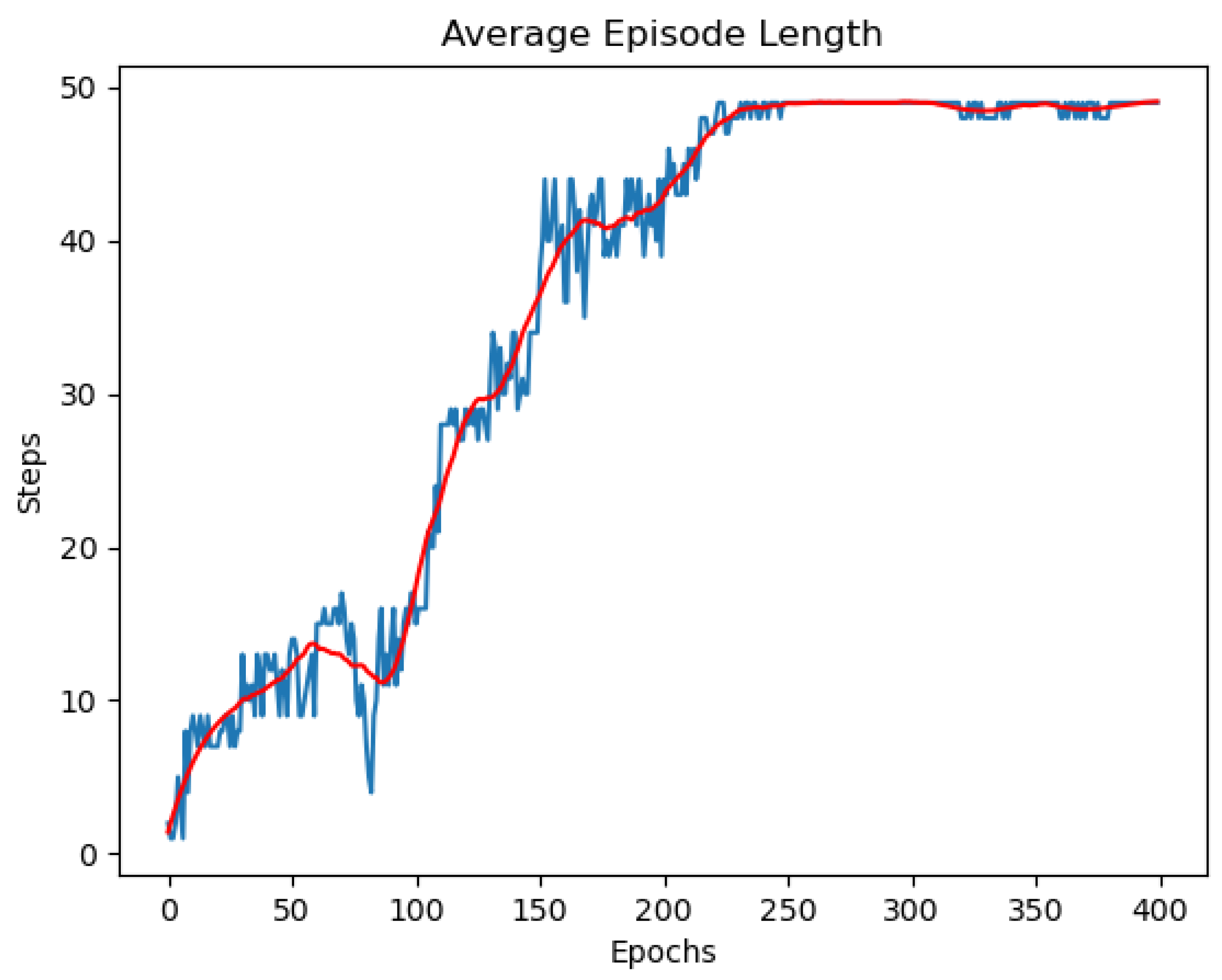
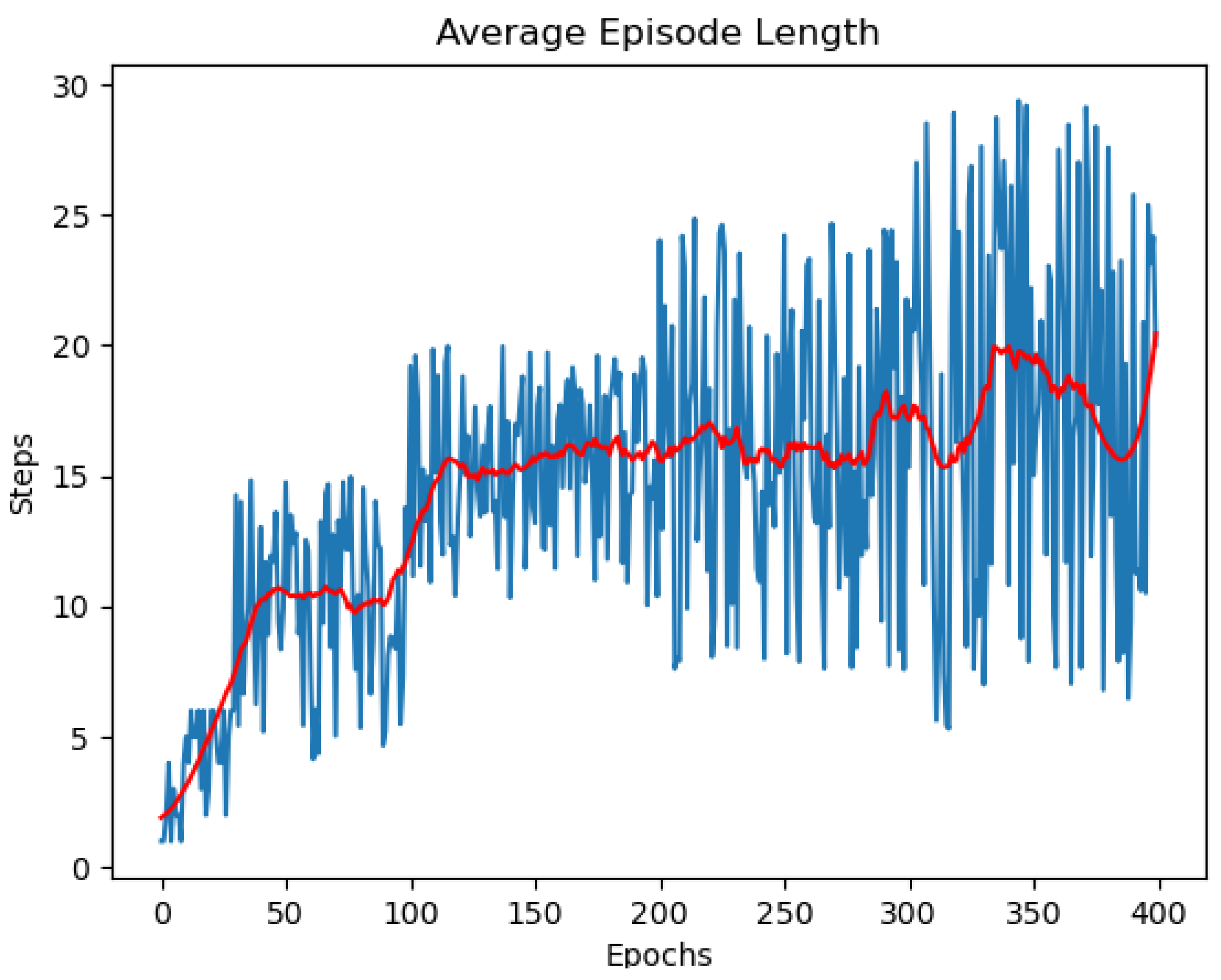
We record the average return and the average episode length to evaluate the agent. For the average episode length, the maximum number of steps per episode is set to 100, as described in Section 4.8. However, if the agent is able to follow the target for 50 consecutive steps, the episode also ends. Figure 8 shows the average episode length when training the DQN agent. We can see that, in the beginning, the agent operates poorly because it was instantiated with random parameters. It usually collides or loses the target and ends the episodes early before reaching 100 steps. After a few more epochs, it learns how to perform the task moderately. Nonetheless, it never reaches 50 steps until the 225th epoch. After that, the agent knows how to keep track of the target consistently and finish the episodes in around 50 steps. This is also the maximum number of consecutive steps that we prescribed above.

On the other hand, it surprises us that the result from the DDPG is much worse. The average episode length of DDPG is illustrated in Figure 9. We can see that the average episode length fluctuates and does not converge. An explanation for this could be that the DDPG is more complicated than the DQN. It has double the number of networks than the DQN; hence, it needs much more epochs to converge. Although we might observe an improvement if the DDPG is trained with more epochs, our goal is not trying to make the DDPG converge but we want to test and choose the better DRL algorithm for the dynamic object tracking task. Being smaller in size, able to converge, and needing a shorter training time, we have enough evidence to show that the DQN outperforms the DDPG in this specific metric.

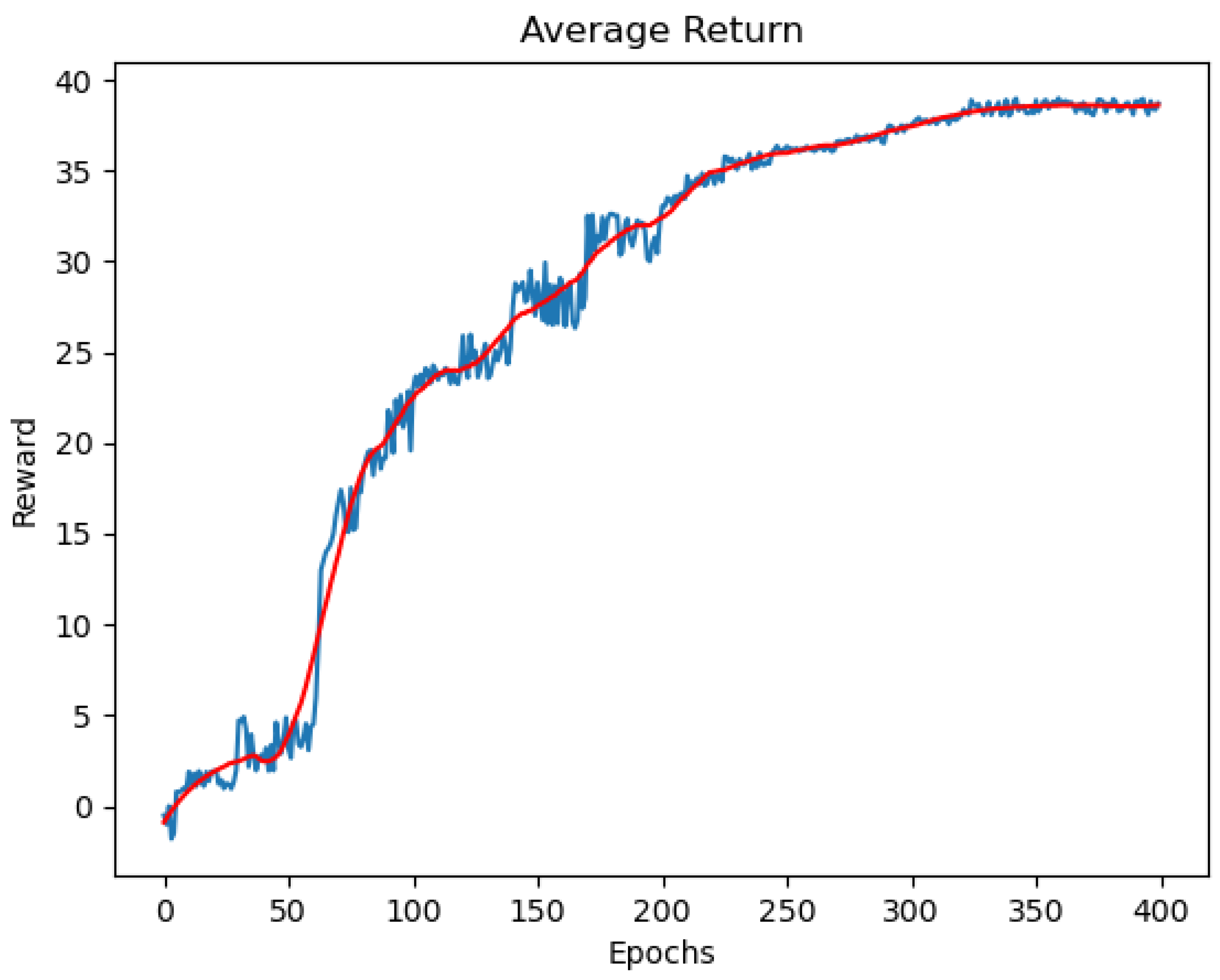
The other metric that we keep track of is the average return. Shown in Figure 10 is the average return of the DQN agent. In the first few epochs, the agent is unable to keep track of the target and usually made collisions; thus, making the average reward low. The reward increases gradually and plateaus at 37 after 300 epochs because at that time, the agent has managed to reach the maximum steps per epoch, as we described above in Figure 8.

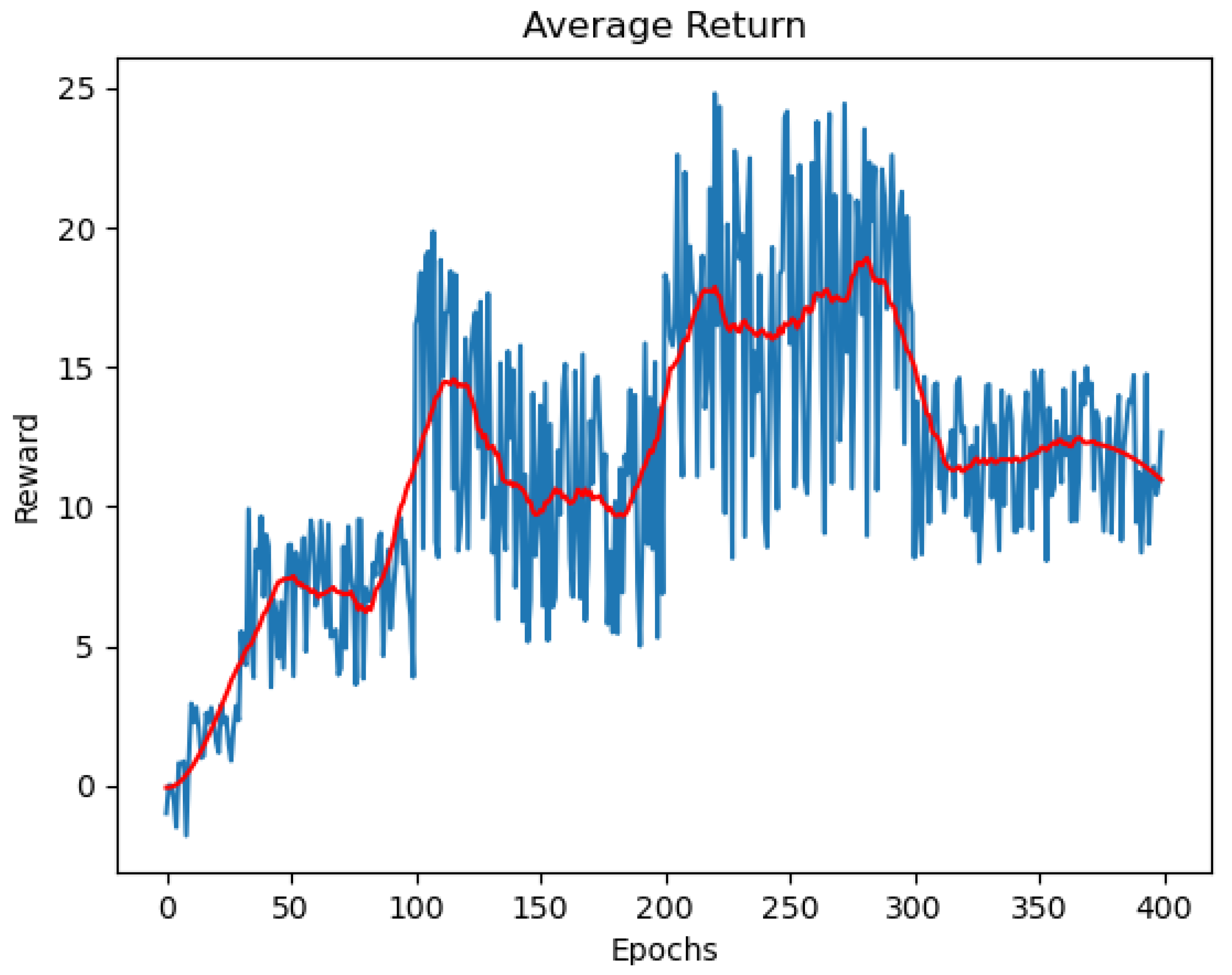
The average return of the DDPG is shown in Figure 11. Identical to the average episode length, the DDPG does not have a good result in this metric as well. Although there is a slight increment in the average reward after a few hundred epochs of training, the result is still very unstable and seems not to be converged. We have tried to alter the hyperparameters (e.g., layer configurations, activation function, CNN kernels, etc.) but none of them show a better result for a DDPG. With all the above results, we can compare and draw some conclusions about the performance of the DQN and DDPG in this dynamic object-tracking task.

After verifying the adaptability of our LDVRL framework to different DRL algorithms, we conduct experiments to examine the simplicity and efficiency of the framework.

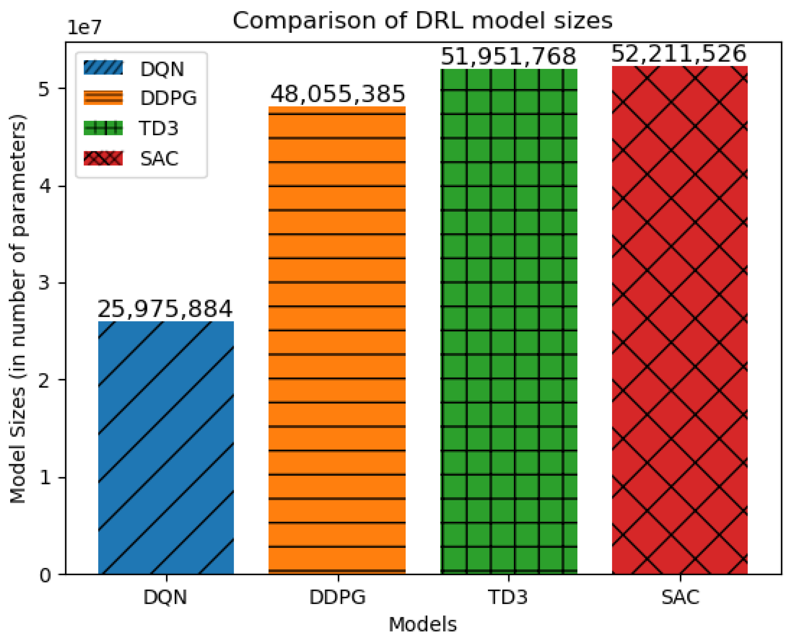
The first experiment is to reason why we chose the DQN. We test different algorithms in our framework (DQN, DDPG, TD3 [32], SAC [33]) and compare the model sizes (in terms of the number of parameters). We use the same network architectures in all algorithms to obtain a fair comparison. It shows that the DQN requires the least computations, and from Figure 10, we can see the DQN still converges and performs well for this task. The DDPG and TD3 have two networks, and the SAC has three networks that result in more parameters compared to the DQN, which has only one network. This experiment consolidates the reason why we chose the DQN as we prioritize the lightweight but effective approach. The exact comparison results can be seen in Figure 12.

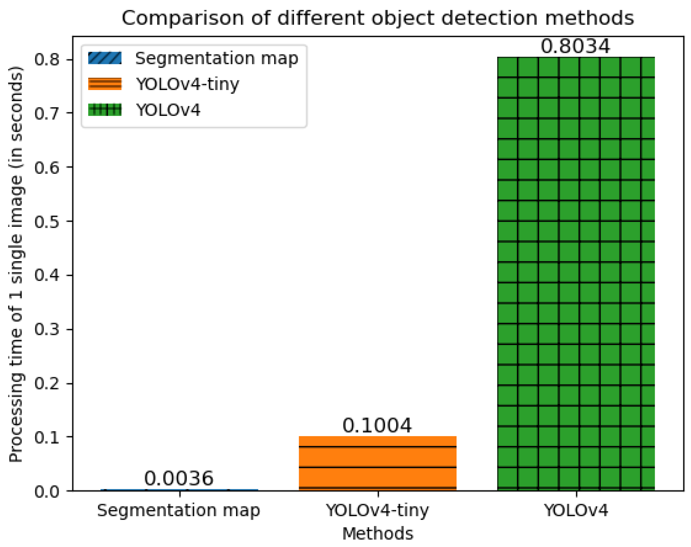
The second experiment is to compare our proposed object detection module with other usual methods. We monitor the processing time required to detect an object and return the bounding box from a single image using three methods: a segmentation map, YOLOv4-tiny, and YOLOv4. The faster the processing time is, the fewer computational resources it requires to complete the task. The recorded processing time is shown in Figure 13. The plot shows that our segmentation map method has the fastest processing time.

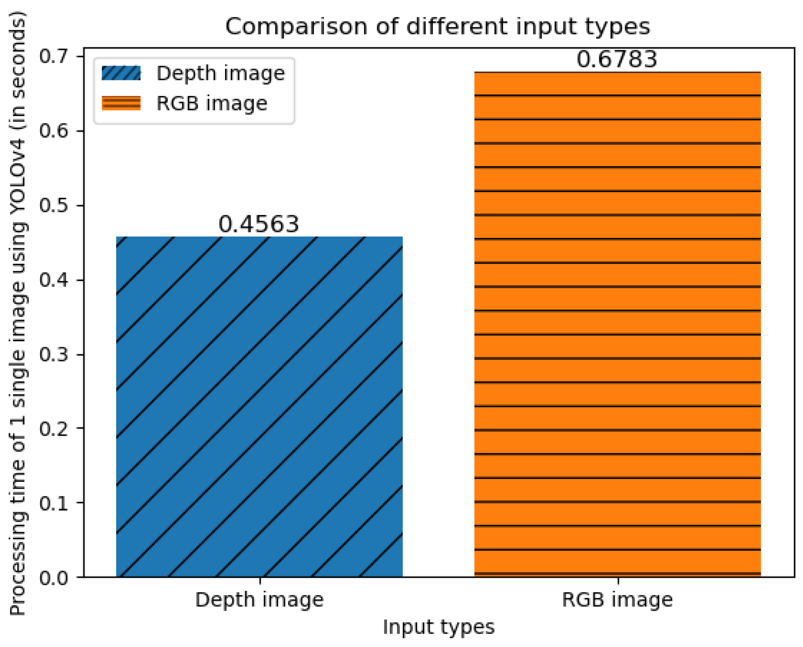
The third experiment shows how much computational cost is reduced when we decide to use depth images instead of RGB images. In this experiment, we compare the processing time of YOLOv4 on a depth image and RGB image. It is clear that depth images have only one channel while RGB images have three. Hence, the number of pixels passed into the CNN of RGB images is triple. The same thing happens when we feed it into the DQN agent. From the experiment, we can see that our framework that uses depth images is not only better for the agent’s prediction ability but also better for reducing the computations needed. The experiment result is shown in Figure 14.

In the fourth experiment, we calculate and compare the time taken to perform a single forward pass (inference time) between our proposed framework and the related conventional methods. Our framework utilizes a DQN as the core DRL algorithm, depth images as our input, segmentation map as the object detection module, and stacks of consecutive frames as our state representation. The alternative framework replaces the segmentation map with the YOLOv4-tiny model for the object detector. This approach is designed for UAVs that are not equipped with segmentation cameras. The conventional method uses a DQN for the DRL algorithm, RGB images as input, YOLOv4 as the object detector, and LSTM to capture the historical movements of the objects. The inference time of the above methods is compared in Figure 1. As we can see from the plot, our proposed framework shows the smallest inference time, which proves its lightweight nature.

6. Conclusions

In this paper, we have demonstrated an autonomous object-tracking system for UAVs using the Lightweight Deep Vision Reinforcement Learning (LDVRL) method. From the experiment and results discussed above, we can see that using the LDVRL method with DQN achieves good performance while maintaining a small model size and can be applied to real-world UAVs whose onboard processing unit is very power limited. We have compared our lightweight techniques with other related conventional techniques to see how much the processing resources are reduced. By using only the visual input captured by the front-mounted camera, the UAVs are not required to equip any additional lasers or sensors to accomplish the task.

We also tested our framework with a DDPG Actor-Critic algorithm and compared it with the DQN. The result shows that the DDPG performs worse than the DQN in this task (with the states in continuous space and actions in discrete space). Our assumption to explain this surprising result is because a DDPG is more complicated with double the number of networks than a DQN. It requires much more work on tuning the parameters as well as more epochs to train. Since our target is to find the most lightweight but effective solution to perform object tracking with an UAV, we did not carry the experiment with the DDPG further. The DQN has shown that it can be trained with fewer epochs and is also smaller in size. Thus, the DQN reduces the required computational resources and is easier to be applied on physical UAVs.

Moving forward, we plan to pursue testing our LDVRL method in real-world scenarios to further validate its efficacy and robustness. This will enable us to refine the system to better handle varying environmental conditions and unexpected challenges. Ultimately, our goal is to create a comprehensive and efficient autonomous object-tracking system for UAVs that is capable of functioning optimally in diverse real-world environments.