Article

Training of Convolutional Neural Networks for Image Classification with Fully Decoupled Extended Kalman Filter

by
Armando Gaytan
1,*,
Ofelia Begovich-Mendoza
1,* and
Nancy Arana-Daniel
2
1
Unidad Guadalajara, Centro de Investigación y de Estudios Avanzados del Instituto Politécnico Nacional, Zapopan 45019, Jalisco, Mexico
2
Centro Universitario de Ciencias Exactas e Ingenierías, Universidad de Guadalajara, Guadalajara 44430, Jalisco, Mexico
*
Authors to whom correspondence should be addressed.
Algorithms 2024, 17(6), 243; https://doi.org/10.3390/a17060243
Submission received: 13 March 2024 / Revised: 11 April 2024 / Accepted: 15 April 2024 / Published: 6 June 2024
(This article belongs to the Special Issue Machine Learning in Pattern Recognition)

Abstract

:
First-order algorithms have long dominated the training of deep neural networks, excelling in tasks like image classification and natural language processing. Now there is a compelling opportunity to explore alternatives that could outperform current state-of-the-art results. From the estimation theory, the Extended Kalman Filter (EKF) arose as a viable alternative and has shown advantages over backpropagation methods. Current computational advances offer the opportunity to review algorithms derived from the EKF, almost excluded from the training of convolutional neural networks. This article revisits an approach of the EKF with decoupling and it brings the Fully Decoupled Extended Kalman Filter (FDEKF) for training convolutional neural networks in image classification tasks. The FDEKF is a second-order algorithm with some advantages over the first-order algorithms, so it can lead to faster convergence and higher accuracy, due to a higher probability of finding the global optimum. In this research, experiments are conducted on well-known datasets that include Fashion, Sports, and Handwritten Digits images. The FDEKF shows faster convergence compared to other algorithms such as the popular Adam optimizer, the sKAdam algorithm, and the reduced extended Kalman filter. Finally, motivated by the finding of the highest accuracy of FDEKF with images of natural scenes, we show its effectiveness in another experiment focused on outdoor terrain recognition.

1. Introduction

Over the past five years, there has been an unprecedented surge in interest in Artificial Intelligence (AI) across various sectors, including industry, research, and modern society [1]. AI applications have become pervasive, encompassing fields such as healthcare, commerce, transportation, logistics, automated manufacturing, finance, entertainment, security, space navigation, and internet services, among many others [2,3,4]. In these applications, Machine Learning stands out as the dominant research area, where Deep Learning models have emerged as the most successful [2,5,6]. The resurgence of neural networks with many hidden layers began in 2006 when a breakthrough combining supervised and unsupervised learning [7] challenged the belief about the great difficulty of training deep networks [8]. This advance sparked renewed research efforts, which led to the development of mechanisms that enabled fully supervised learning. These mechanisms took advantage of backpropagation and gradient descent for the training process [7,8,9].
Since then, novel algorithms have surfaced, primarily emphasizing the refinement of gradient gain for synaptic weight updates. While these optimizers boast advantages over traditional methods, yielding remarkable results in specific scenarios, they need extensive training datasets and many iterations to attain the desired learning thresholds. Moreover, their efficacy often diminishes when confronted with intricately complex problems. Thus, research in this field remains open and ongoing [10].
In addition to these algorithms based on gradient descent, there are learning methods that incorporate second-order information that has shown superior accuracy compared to first-order algorithms, often achieving satisfactory results in fewer training epochs. However, its considerable computational demands pose a challenge, especially when dealing with deep networks, due to the large number of adjustable parameters. Consequently, they are applied in small neural networks [9,11,12].
The Extended Kalman Filter (EKF) incorporates second-order information through the estimation error covariance. This method was introduced to neural network training in 1988 by Singhal and Wu [13]. Their pioneering work demonstrated that the EKF converges in fewer iterations and with higher accuracy than backpropagation. Subsequently, two publications [11,14] provided evidence of these advantages but pointed out the greater computational complexity.
Then new versions of the EKF appeared, the most immediate in [14], with the idea of multiple EKF units (MEKA), where each MEKA unit is applied to a specific group of weights of the neural network, operating independently. Meanwhile, in [11], Puskorius and Feldkamp developed a scheme with a single EKF for the entire neural network, which is compatible with scenarios where uncorrelated weights exist in the neural model. This approach, unlike MEKA, aligns with the original EKF and offers substantial computational relief without compromising accuracy. The general model is known as the decoupled extended Kalman filter (DEKF).
The authors of the DEKF propose different decoupling levels: the global extended Kalman filter (GEKF) considers that all weights are correlated; layer-decoupled extended Kalman filter (LDEKF) assumes that the weights within each layer are correlated but not with weights in other layers; node-decoupled extended Kalman filter (NDEKF) correlates the weights of the afferent connections of each neuron; and fully decoupled extended Kalman filter (FDEKF) omits any correlation between weights [11].
In the early development of the EKF as a training algorithm, it was applied to multilayer perceptron neural networks for pattern classification problems. However, the networks that were used in these cases consisted of just a few layers and neurons [13,15]. Nowadays, taking advantage of modern computational hardware, the algorithms based on the EKF seem interesting for training neural networks with many weights. For example, in [16], the authors of this paper have performed a comparison of the NDEKF against the Adam optimizer on the function approximation with multilayer neural networks. The NDEKF has shown faster convergence, in the number of epochs, and has led to higher accuracy.
In this research, we are interested in investigating the convergence speed, in terms of the number of epochs, of the FDEKF with deep convolutional neural networks (DCNNs), as well as its performance in scenarios where first-order optimizers struggle to achieve high accuracy. This evaluation aims to provide compelling evidence of the superiority of the FDEKF in accuracy and speed.
Furthermore, the high degree of decoupling inherent to the FDEKF enhances its suitability for neural networks with a multitude of synaptic weights. Consequently, the application of FDEKF in the training of DCNNs becomes a promising prospect.
The primary objective of this research is to investigate the effectiveness of the FDEKF as a training algorithm for DCNNs in the context of solving image classification problems. To assess our initial hypothesis, we will conduct a comprehensive comparison of the FDEKF algorithm against the three others, which are explained in Section 4: Adam Optimizer [17], sKAdam [18], and Reduced-EKF (REKF) [19].
In past research, the EKF and its variations have been used in multilayer perceptron neural networks that have one or two hidden layers with a limited number of neurons [11,13,14,20]. In this work, for the first time, the FDEKF is applied to DCNNs.
In this research, we faithfully apply the FDEKF algorithm following [11], ensuring that it complies with the recursive nature of the EKF. Updating the weights occurs on a sample-by-sample basis, thus maintaining the conditions for the stability analysis outlined in [21].
The data sets selected for our experiments have been used in other image classification works. We develop three experiments to test the performance of the FDEKF against other algorithms and another experiment to apply the FDEKF to terrain recognition to generate a cost map of its traversability.
The main contributions of this article are to show the feasibility of the FDEKF for training DCNNs, the superiority of training with FDEKF in the speed of convergence concerning the number of epochs, and the higher precision in the early training phase. These findings are anticipated to spark greater interest in exploring the EKF as a viable training algorithm for DCNNs.
With this article, we want to show the scientific community that the FDEKF is a good strategy for DCNNs training. The FDEKF is a second-order algorithm with some advantages over the first-order algorithms, so it can result in faster convergence and lead to higher accuracy due to a higher probability of finding the global optimum. The FDEKF largely preserves the behavior of the EKF, even neglecting the statistical correlation between some pairs of elements of the synaptic weight vector, benefiting from a reduction in computational complexity.
The structure of this work is organized as follows: In Section 2, we provide a concise overview of DCNNs in the context of image classification and describe critical aspects of the training process. Section 3 presents an exhaustive description of the FDEKF model, starting from the EKF and including the key considerations for its application in the training of neural networks. Section 4 provides a brief overview of the algorithms within our framework, namely Adam, sKAdam, and REKF, which have been explored in previous related works. In Section 5, we present the results and details of the experiments performed in this study. Finally, we draw our conclusions and provide information on possible avenues for future research.

2. Deep Convolutional Neural Networks in Image Classification

The first neural network model with convolutional layers, named Neocognitron by Fukushima, its author, dates from 1979 and was inspired by the hierarchical biological model of the visual nervous system proposed by Hubel and Wiesel in the 1960s. In this model, neurons from deeper layers tend to respond selectively to more complicated features of the stimulus pattern, have a larger receptive field, and are more insensitive to variations in position compared to neurons from earlier layers [22,23].
In 1989, LeCun presented the first convolutional network with learning through the backpropagation method by applying the gradient descent rule [24]. However, in the following years, there was a consensus among researchers about the difficulty of applying backpropagation for deep networks, mostly due to the problem of gradient vanishing and exploding [8,23].
In 2006, Hinton et al. [7] found a combination of unsupervised and supervised learning, which again encouraged research into learning in multilayer neural networks. This work meant the renaissance of deep learning [8,10,23]. Subsequently, various contributions enabled fully supervised learning in DCNNs. We refer to regularization and normalization mechanisms, features of network architecture, nonlinear activation functions, supervision components, optimization techniques, and strategies to reduce the computational cost [8,10,23,25].
In 2012, for the first time, a DCNN model outperformed other machine learning techniques in image classification tasks [26,27]. Since then, this type of problem has been solved better with DCNNs than with any other category of machine learning, surpassing even the precision of human perception [8,9,10].
The power of a DCNN lies fundamentally in its convolutional layers. This kind of layer works as a set of local receptive fields extracting information at a certain level of abstraction according to the location of the layer in the depth of the network [9,23]. In convolutional layers, the adjustable weights are organized into two-dimensional sub-sets, a filter bank, which are convolved with the input to the layer, which also occurs in two dimensions per channel. Due to the nature of the convolution operation, the synaptic weights turn out to be shared, with the benefit of a lower count of them compared with an equivalent layer of a multilayer perceptron network [8,10,23]. A detailed explanation of the operation of convolutional layers can be found in [10,23].
A convolutional layer is typically followed by rectified linear units (ReLU) instead of traditional sigmoidal functions like logistic or hyperbolic tangent [27]. Unlike these, which tend to saturate in certain regions, ReLU maintains a non-saturating behavior in the positive region. This characteristic plays a crucial role in mitigating the vanishing gradient problem, a common obstacle in the training of DCNNs. Remarkably simple ReLU has a profound impact on the training process [27]. Its simplicity translates into computational efficiency and ease of differentiation, contributing to faster training compared to more intricate activation functions. Some researchers have explored certain varieties, and sometimes outcomes have slight improvements, but they have not deviated significantly from the widespread adoption of ReLU [10,23]. A comprehensive overview of these alternatives can be found in [10]. The three activation functions mentioned above are shown in Figure 1.
Towards the end of a DCNN, fully connected layers are usually found; these operate as a conventional layer of multilayer perceptron networks, omitting the activation function, that is, performing the powered sum. The fully connected layers that follow these layers interpret these feature representations and perform the function of high-level reasoning [10]. In the final layer, for the classification task, the softmax operation is usually performed, which contributes to forcing better precision in class separation and consists of a normalization mode through the exponential function [10,23].
Given the large dimension of the output of a convolutional layer, due to both the input size and the number of filters used, additional subsampling is often necessary. Maxpooling has become the preferred technique for this purpose as it achieves not only subsampling but also invariance to translation, rotation, and scaling of features extracted from the previous convolutional layer [10,23,28,29]. This operation extracts information from each subimage of an image coming from the convolutional layer and represents it with a single value at a specific position in the resulting image. The dimension of each subimage is determined by the size of the corresponding pooling filter, and dimension reduction is achieved through a scanning process that skips rows and columns. In maxpooling, the representative value is the maximum among the values within the subimage. Although alternative operations such as averaging, a hybrid approach, p-norm, and others have been explored, maxpooling and average-pooling stand out as the most widely used methods [23]. For detailed information on these variants, see [10,28].
Towards the end of a DCNN, fully connected layers are usually found; these operate as a conventional layer of multilayer perceptron networks, omitting the activation function, that is, performing the powered sum. The fully connected layers that follow these layers interpret these feature representations and perform the function of high-level reasoning [10]. In the final layer, for the classification task, the softmax operation is usually performed, which contributes to forcing better precision in class separation and consists of a normalization mode through the exponential function [10,23]. The following equation shows the softmax function.
f ( x i ) = e x i j = 1 n e x j for i = 1 , 2 , , n , and x = [ x 1 , , x n ] T R n .
In the image classification task, DCNN is the most used architecture, such as ResNet-50, VGG-16, VGG-19, and Inception-v3 [30], except for problems with small data sets in which it is preferable a support vector machine [31]. Generally, its training is through backpropagation, a method by which the gradient of an objective function, such as a loss function, determines the adjustment of the trainable parameters of the neural network to minimize the class identification error [10,29].
The DCNN models used in our experiments are built with layers of the different classes described in this section and are applied in image classification tasks that, as read in the previous paragraph, are usually trained by backpropagation using a first-order optimizer. This research includes the most popular first-order optimizer among the algorithms with which it compares the performance of FDEKF.

3. Fully Decoupled Extended Kalman Filter

This section begins by explaining the EKF as a training algorithm for neural networks, which serves as the fundamental concept behind the FDEKF. Subsequently, the distinctive aspects that define and characterize the FDEKF are delved into.

3.1. Extended Kalman Filter

Following the introduction of the Kalman filter (KF) in 1960, applicable to linear systems exposed to random noise, for smoothing, filtering, or prediction [32], the EKF emerged in 1961 [33]. The EKF was developed for nonlinear systems, and despite not ensuring an optimal estimate, the EKF consistently delivers remarkable results [13]. In our context, the EKF is implemented in a neural model for the estimation of the system state, which contains the synaptic weights and the biases. Consequently, it deals with a discrete-time nonlinear dynamic system where the output is given by a nonlinear function of the state vector y at the entrances. In general, the nonlinear model in discrete time is represented by the following equations:
x k + 1 = f ( k , x k ) + w k ,
y k = h ( k , x k ) + v k ,
where x k + 1 is the state at instant k + 1, x k is the current state, y k is the measurable output, f ( · ) is the state transition function, and h ( · ) is the measurement nonlinear function, with w k and v k representing additive white noise in the process and in the measurement, respectively.
The process begins with the initialization of the filter:
x ^ 0 = E [ x 0 ] ,
P 0 = E [ ( x ^ 0 E [ x 0 ] ) ( x ^ 0 E [ x 0 ] ) T ] ,
where E [ · ] denotes expected value, and for the initial instant: x 0 is the state, x ^ 0 is the estimated state, and P 0 is the error covariance matrix.
Then the same iterative operations of the KF are performed, incorporating the pair of linearization operations additionally required by the EKF:
F k + 1 , k = f ( k , x k ) x | x = x ^
H k + 1 , k = h ( k , x k ) x | x = x ^
The iterative computation continues with the propagation of the state estimator to obtain x ^ k , a priori state estimate:
x ^ k = f ( k , x ^ k 1 ) ,
the propagation of the covariance of the estimation error to obtain P k , a priori estimation error covariance matrix:
P k = F k , k 1 P k 1 F k , k 1 T + Q k 1 ,
where Q k 1 is the covariance matrix of the noise in the process at k − 1, then the computation of the Kalman gain matrix K k :
K k = P k H k T [ H k P k H k T + R k ] 1 ,
where R k is the covariance matrix of the noise in the measurement at k, then the state estimate correction:
x ^ k = x ^ k + K k ( y k h ( k , x ^ k 1 ) ) ,
and finally, with I being the identity matrix of the same size as P k , the error covariance correction:
P k = ( I K k H k ) P k .
In this way, the EKF recursive procedure serves as the basis for a second-order neural network training approach. The estimation error covariance matrix, which evolves throughout the process, is essential to the performance of the EKF, as it encodes second-order information about the training problem [15].
The EKF as a training algorithm was initially proposed for multilayer perceptron-type neural models, proving to be more effective in terms of the number of training epochs than standard backpropagation for a series of pattern classification problems.

3.2. Fully Decoupled Extended Kalman Filter

In the EKF for training neural networks, the computational requirements are mainly determined by the storage and updating needs of the estimation error covariance matrix. If the network has M weights and N o outputs, the computational complexity is O( N o M 2 ) and the storage requirements are O( M 2 ) [15].
Although the EKF stands out for its accuracy and faster convergence in terms of epochs, it is impractical in large neural networks [21]. To reduce the computational burden, Puskorius and Feldkamp [11] introduced a modified EKF approach in 1991. This variant simplifies computations by disregarding statistical correlations between network parameters across different groups, operating under the assumption that each parameter solely correlates with others within the same group. Therefore, the complexity is O( N o 2 M + N o i = 1 g M i 2 ), where M i is the number of weights in the group i, and the storage need is O( i = 1 g M i 2 ). The computational complexity and computational requirements are significantly lower than with the EKF. On the other hand, although the EKF calculations are performed for each group, the scaling matrix, whose inverse is required for calculating the Kalman gain, is unique and must be previously calculated in each iteration.
Different forms of grouping can be assumed: a group for each layer of the network or layer-decoupled (LDEKF), a group for each node, or node-decoupled (NDEKF), and groups with only one element, or fully-decoupled (FDEKF); at the other extreme, there is a single group approach, which preserves the assumption of the EKF, referred to by the authors as the global group (GEKF).
These authors mention the advantage of significantly reducing the computational load with little sacrifice of the performance of the trained network. The NDEKF approach appears to be the most natural, is consistent with the original EKF, and offers a good balance between computational complexity and accuracy. NDEKF has exhibited exceptional convergence characteristics and generalization capabilities, even outperforming GEFK, according to an experiment described in [34]. With decoupling, the estimation error covariance matrix becomes block diagonal for NDEKF and LDEKF, while for FDEKF it is absolute diagonal. Figure 2 shows a representation, similar to one shown in [11], of four different levels of decoupling. If we think about the error covariance matrix, we see that the white positions contain zeros and the gray positions contain non-zero values.
On the other hand, taking advantage of the computational processing speed of currently available hardware, the FDEKF algorithm is now feasible for the complete training of multilayer neural networks with a large number of weights. Despite the disregard of statistical correlation between network parameters, FDEKF offers very good performance with much lower computational complexity.
To apply any of the variants of the EKF to neural networks, it is assumed that there is a stationary neural model with ideal weights. These make up the state of the system that is attempted to be estimated through the application of the EKF. The response of the model is the output of the neural network. The ideal weights, which are kept constant, are those that minimize the error between the network output and the target output for the entire data set.
In practice, it is argued that the introduction of noise into the process favors the performance of the filter [35]. The behavior of a neural network can be represented by the following discrete-time nonlinear dynamic system:
θ k + 1 = θ k + w k ,
y k = h k ( θ k , u k ) + v k ,
where θ k is the system state vector, which contains the synaptic weights of the neural network, u k is the neural network input, y k is the neural network output, h k ( · ) is a nonlinear function of synaptic weights and input, w k and v k are additive Gaussian white noise in the process and the measurement, respectively. The process equation depicts that the state of the ideal neural network is characterized as a steady state corrupted by noise. The observation or measurement equation represents the desired response vector of the network as a nonlinear function of the input vector and the state vector, plus the measurement noise. This noise and that of the process are characterized by a zero mean with covariance specification, thus:
E w k w l T = Q k , k = l 0 , k l ,
E v k v l T = R k , k = l 0 , k l .
In [15], the introduction of process noise is justified as a simple and easily controlled mechanism that helps ensure that the error covariance approximation matrix can retain the necessary property of being non-negatively definite and, in this way, avoid divergence problems. These authors also found that, if chosen carefully, it helps speed up the training process and, more importantly, produces a better performance of the trained network, besides referring to the other three research studies that also found benefits from introducing process noise. The authors of reference [35] state that it is often advantageous to add noise to the model to force the filter to continually adjust the weights and prevent the Kalman gain from going to zero. In some training algorithms, gradient-based learning also exploits the benefits of process noise. In [21], to efficiently implement the filter, noise is artificially introduced into the process, with a diagonal matrix as covariance. Many prefer to use the identity matrix multiplied by a very small value [19], as an example, in [36] the noise covariance is I · 10 6 , where I is the identity matrix. Instead, few researchers [13,37] do so without the introduction of noise in the process. However, one can also think of the neural model of optimal weights without noise in both the process and the measurement [38].
Regarding the noise in the output, although it is common to use constant diagonal covariance, it seems convenient to update during the training. Chapter 7 of [12] states that measurement noise in the EKF affects convergence speed and performance. The authors recommend using a diagonal covariance matrix and gradually decreasing the values as the training process progresses, being able to update based on the error covariance. A different way to update them is based on a weighted sum of the previous value and another value dependent on the magnitude of the weight update. In [13] it uses an initial value I (identity), and the magnitude of the noise covariance of the measurement is exponentially reduced through the function I · e k / 50 , with k denoting the epoch number in the course of training. In [21] is similar, but with an exponential decay factor determined based on the total number of epochs, to conclude with a very low power noise; for [21] this cancels out the noisy behavior of the filter as it approaches the minimum. In Chapter 5 of [12], the general recommendation is to use a scaled identity matrix, either the scaling factor is kept constant during training or it is updated keeping directly proportional to the cost function, thereby that its value decreases as training improves.
In Algorithm 1, it is shown the pseudocode for FDEKF [11]:
Algorithm 1 FDEKF
Require:  P 0 : Initialize diagonal matrix of estimation error covariance
Require:  Q 0 : Initialize diagonal matrix of process noise covariance
Require:  R 0 : Initialize measurement noise covariance
Require:  θ 0 : Initial parameter vector
t ← 0. Initialize timestep
while  θ t not converged do
   tt + 1
    H t θ y t ( θ t 1 ) . Get gradients of network output w.r.t. the parameters at timestep t
    P t | t 1 P t 1 | t 1 + Q 0 . Compute a priori state estimation error covariance
    S t H t P t | t 1 H t T + R t 1 . Compute output estimation error covariance
    K t P t | t 1 H t T S t 1 1 . Compute Kalman gain
    θ t θ t 1 + K t ( y t * y t ) . Update parameters
    P t | t ( I K t H t ) P t | t 1 . Compute a posteriori state estimation error covariance
    R t . Applying a measurement noise covariance update rule
end while
return θ t . Resulting parameters

4. Previous Related Work

4.1. Adam Optimizer

In 2015, Kingma and Ba introduced Adam [17], a first-order gradient-based optimization algorithm for stochastic objective functions. Adam has gained significant popularity in the training of DCNNs. This algorithm, derived from adaptive moment estimation, amalgamates the strengths of its predecessors, AdaGrad and RMSProp [17].
Regarded as one of the most extensively used optimizers in neural network training, Adam has shown superior performance than other first-order algorithms [19]. Although various adaptations of the Adam optimizer have emerged attempting to enhance its performance, such as the strategy proposed by Dubey et al. [39], that modulates learning speed when gradients exhibit minimal differences compared to preceding iterations, Adam remains the prevailing choice in DCNNs.
The method calculates adaptive learning rates tailored to each parameter by estimating the first and second moments of the gradients, relying solely on the computation of first-order gradients. As described by the authors, Adam offers several advantages: it maintains parameter update magnitudes regardless of gradient rescaling, confines step sizes approximately within the step size hyper-parameter range, operates without necessitating a stationary objective, accommodates sparse gradients, and inherently executes a form of annealing of step size [17].
The algorithm updates the exponential moving averages of the gradient and the squared gradient, where the hyper-parameters β 1 , β 2 [ 0 , 1 ) control the exponential decay rates of these moving averages. The moving averages themselves are estimates of the first moment (the mean) and the second raw moment (the uncentered variance) of the gradient.
The authors recommend this hyper-parameter setting for machine learning problems: α = 0.001 , β 1 = 0.9 , β 2 = 0.999 , and ϵ = 10 8 ) .
In Algorithm 2, it is shown the pseudocode for the Adam Optimizer [17], where all operations on vectors are element-wise.
Algorithm 2 Adam Optimizer [17]
Require:  α : Stepsize
Require:  β 1 , β 2 [ 0 , 1 ) : Exponential decay rates for the moment estimates
Require:  f ( θ ) : Stochastic objective function with the parameters θ
Require:  θ 0 : Initial parameter vector
m 0 0 (Initialize 1st moment vector)
v 0 0 (Initialize 2nd moment vector)
t 0 (Initialize timestep)
while  θ t not converged do
    t t + 1
    g t θ f t ( θ t 1 ) (Get gradients w.r.t. stochastic objective at time-step t)
    m t β 1 · m t 1 + ( 1 β 1 ) · g t . Update biased 1st moment estimate t
    v t β 2 · v t 1 + ( 1 β 2 ) · g t 2 . Update biased 2nd raw moment estimate t
    m ^ t m t / ( 1 β 1 t ) . Compute bias-corrected 1st moment estimate
    v ^ t v t / ( 1 β 2 t ) . Compute bias-corrected 2nd raw moment estimate
    θ t θ t 1 α · m ^ t / ( v ^ t + ϵ ) . Update parameters
end while
return θ t . Resulting parameters

4.2. sKAdam Optimizer

The sKAdam algorithm, introduced in [18], derives its name from the fusion of the scalar Kalman filter and the Adam optimizer. Notably different from the FDEKF, this implementation of the EKF manifests two significant distinctions. Firstly, it does not serve directly as a learning algorithm; rather, it functions to filter the gradient obtained through backpropagation while the learning process is facilitated by the Adam Optimizer. Secondly, the scalar Kalman filter allocates a separate filter to each component of the gradient, also distinguishing itself in this sense from the FDEK.
The sKAdam algorithm has its origins in the KAdam algorithm, introduced earlier by the same authors. KAdam operates with filter sets, assigning a group for each layer within the neural network. However, unlike KAdam, the approach in sKAdam involves employing 1-D Kalman filters for each parameter within the loss function. Furthermore, the measurement noise covariance is forced to drop exponentially as the training process progresses with the sKAdam algorithm. As a consequence of these modifications, sKAdam develops scalar operations instead of calculations with matrices and vectors, and on the other hand, the decreasing noise allows for achieving lower values in the loss function [18].
The authors claim that the filter can add significant and relevant variations to the gradient, causing a similar effect to the strategy of adding white noise to the gradient that other researchers have implemented to improve learning in very deep neural networks to find better solutions in the function of loss [18].
For hyper-parameter configuration in sKAdam, the same recommendations are made as for Adam, where applicable. For the filter model, the authors make conventional recommendations, plus the particularity of the exponential decay factor of the measurement noise covariance.
In Algorithm 3, it is shown the pseudocode for sKAdam [18].
Algorithm 3 sKAdam Optimizer [18]
Require:  α : Stepsize
Require:  β 1 , β 2 [ 0 , 1 ) : Exponential decay rates for the moment estimates
γ : Exponentially decay constant for the measurement noise
Require:  f ( θ ) : Stochastic objective function with parameters θ
Require:  θ 0 : Initial parameter vector
m 0 0 (Initialize 1st moment vector)
v 0 0 (Initialize 2nd moment vector)
x ^ 0 | 0 0 (Initialize state estimates vector)
k 0 0 (Initialize Kalman gains vector)
p 0 | 0 0 (Initialize covariances vector)
t 0 (Initialize timestep)
while  θ t not converged do
    t t + 1
    g t θ f t ( θ t 1 ) . Get gradients of stochastic objective w.r.t. parameters at timestep t
    x ^ t | t 1 x ^ t 1 | t 1 . Compute a priori state estimate
    p t | t 1 p t 1 | t 1 + 1 . Compute a priori covariance
    r t e t / γ . Compute measurement noise
    k t p t | t 1 / ( p t | t 1 + r t ) . Compute Kalman gain
    x ^ t | t x ^ t | t 1 + k t · ( g t x ^ t | t 1 ) . Compute a posteriori state estimate
    g ^ t x ^ t | t . Set estimated gradient
    p t | t p t | t 1 k t · p t | t 1 . Compute a posteriori covariance
    m t β 1 · m t 1 + ( 1 β 1 ) · g ^ t . Update biased 1st moment estimate t
    v t β 2 · v t 1 + ( 1 β 2 ) · g ^ t 2 . Update biased 2nd raw moment estimate t
    m ^ t m t / ( 1 β 1 t ) . Compute bias-corrected 1st moment estimate
    v ^ t v t / ( 1 β 2 t ) . Compute bias-corrected 2nd raw moment estimate
    θ t θ t 1 α · m ^ t / ( v ^ t + ϵ ) . Update parameters
end while
return θ t . Resulting parameters

4.3. REKF

The reduced extended Kalman filter (REKF) is a pioneering training algorithm in applying to DCNNs any variety of the EKF [19]. This method combines the EKF version adapted for batch training and the use of a scalar error measure, both initially proposed in [15]. The derivation of the scalar error involves incorporating the calculation of the cost function as the output of the neural model exclusively for training purposes.
In Algorithm 4, it is shown the pseudocode for REKF [19].
Algorithm 4 REKF [19]
Require:  P 0 : Initialize a vector with the estimation error covariances
Require: q: process noise covariance, same for all parameters
Require: r: measurement noise covariance, scalar value
Require:  θ 0 : Initial parameter vector
t ← 0. Initialize timestep
while  θ t not converged do
   tt + 1
    H t θ L t ( θ t 1 ) . Get gradients of loss function w.r.t. the parameters at timestep t
    P t | t 1 P t 1 | t 1 + q. Compute a priori state estimation error covariance
    s t s u m ( P t | t 1 H ( i ) t H ( i ) t ) + r t 1 . Compute the total scalar value of innovation
    P t | t P t | t 1 K t H t P t | t 1 . Compute a posteriori estimation error covariance
    K t P t | t 1 H t T s t 1 1 . Compute Kalman gain
    θ t θ t 1 K t L t ( θ t 1 ) . Update parameters
end while
return θ t . Resulting parameters
In [19], the REKF algorithm is described as similar to the FDEKF, even though training is performed in batches without specifying the precise method for accumulating gradients and errors obtained from individual samples within each batch. Different from FDEKF, which is applicable for sample-by-sample training. Regarding the above, it is important to note that to properly apply EFK variants in batch training, synaptic weight adjustments do not depend on the average of the modifications calculated from individual training pairs within the batch. The correct calculation methodology is exhaustively explained in [15], aligning with the recursive nature of the EKF.

5. Experiments

Our primary objective is to evaluate the efficacy of the FDEKF algorithm within DCNNs. To achieve this, we conducted three experiments utilizing widely recognized datasets for classification tasks: fashion images, sports images, and the MNIST Hand-written Digits dataset. These datasets are available in the public access repositories of TensorFlow and GitHub. A visual representation of these datasets is depicted in Figure 3.
The images at the center of Figure 3 encompass a wide array of sports scenes captured within a natural environment and have low spatial resolution, thereby presenting a notably more challenging classification task compared to the other experiments. The samples of the other two experiments, positioned to the left and right of the figure, feature schematic images and plane traces.
The experiment with the set of images that involves scenes and scenarios of sports practice is a test that we relate to the possibility of addressing terrain recognition problems. The performance of the FDEKF in the recognition of such outdoor images represents a precedent for the task of training a neural network for terrain recognition, intending to develop a cost map of traversability for autonomous navigation purposes, our last experiment.
In the first three experiments, which are of image classification, the neural network architecture includes three convolutional layers of 20 kernels size 5 × 5 in the first convolutional layer and 20 kernels size 3 × 3 in the other convolutional layers. The characteristics of the neural network architecture were determined heuristically, resulting in a network of similar magnitude to the architectures used in [19], which are the first experiments with an algorithm EKF-based applied to DCNNs. In the experiments with each set of images, the training process was carried out ten times, so the results shown in the graphs represent the average performance over those ten runs.
In those experiments, for comparison purposes, FDEKF uses the average loss value of every 256 samples, which is the batch size for the other algorithms.

5.1. FASHION Classification Experiment with DCNN

Data set with images of clothing: 60,000 pairs in the training data set and 10,000 for testing. They are available through the TensorFlow module: tf.keras.datasets.fashion_mnist. The entries to the neural network are of dimension 28 × 28, corresponding to grayscale images, to classify them into ten different classes. The DCNN has the characteristics that were described at the beginning of this section.
Ten training processes of three epochs are executed with each of the algorithms: Adam, SKAdam, REKF, and FDEKF. Batch size is 256, except for FDEKF. The loss function is the mean squared error (MSE). For REKF: P 0 = I , Q 0 = I · 10 5 , R = 1 . For FDEKF: P 0 = I · 5 × 10 2 , Q 0 = I · 10 8 , R 0 = 2 × 10 2 , R is adjusted every 256 samples based on the average of values in P of the output node. Hyper-parameters settings for Adam and sKAdam: α = 0.001 , β 1 = 0.9 , β 2 = 0.999 , and ϵ = 10 8 .
The evolution of the loss function with each of the algorithms is shown in Figure 4. The graph depicts the loss value calculated at each iteration of the training process. The value of the loss function decays much faster with FDEKF. From the first iteration, after 256 training samples, the loss function decays rapidly with FDEKF. The performances of Adam and sKAdam are very similar to each other, both in the evolution of the loss function and in precision. Consistently, with these results, Table 1 shows the greatest accuracy of FDEKF.

5.2. SPORTS Classification Experiment with DCNN

Data set with images of different sports; from here, 30,000 pairs have been taken for training and 5000 for testing. The neural network is DCNN, the same as the previous experiment, except for the dimension of the input layer: 21 × 28. The entries are grayscale images to classify into ten different classes. This is the experiment in that the low spatial resolution of the images, as well as the fact that they capture a moment of sports practice, makes the task of recognition more difficult.
Ten training processes of three epochs are executed with each of the algorithms. Batchsize 256, except for FDEKF. The loss function is MSE. For REKF: P 0 = I , Q 0 = I · 10 5 , R = 1 . For FDEKF: P 0 = I · 5 × 10 3 , Q 0 = I · 10 8 , R 0 = 10 3 , R is adjusted every 256 samples based on the average of values in P of the output node. Hyper-parameter settings for Adam and sKAdam: α = 0.001 , β 1 = 0.9 , β 2 = 0.999 , and ϵ = 10 8 .
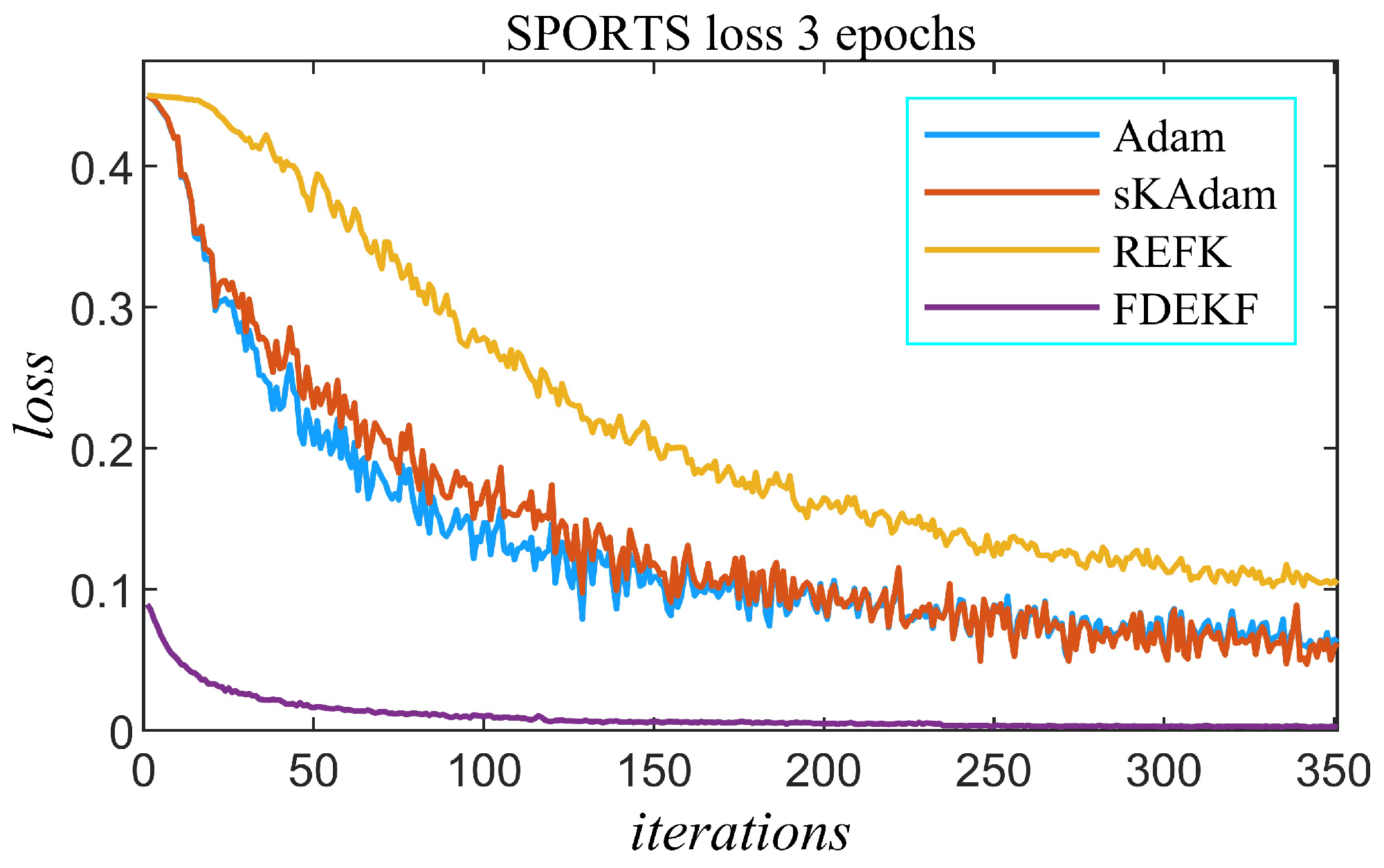
In this experiment, as in the previous one, with FDEKF, the value of the loss function decays much faster in the training process, and the highest precision is obtained for the test data set, as observed in Figure 5 and Table 2, respectively. Here, the advantage of FDEKF over other algorithms in precision is greatest. This result supports one of our hypotheses, that with FDEKF, high precision can be achieved in image recognition tasks in which first-order algorithms do not.

5.3. MNIST Classification Experiment with DCNN

This experiment is with the MNIST database, which contains handwriting digits, one of the most widely used references to test image classification methods, generated by LeCun et al. [40], available at http://yann.lecun.com/exdb/mnist/, accessed on 3 December 2022, in its original dimension. The neural network is a DCNN identical to the one in the first experiment. The training data set has 60,000 original image samples of 28 × 28 pixels, while the test data has 10,000 images with the same characteristics.
Ten training processes of three epochs are executed with each of the algorithms. Batchsize 256, except for FDEKF, which is sample to sample. The loss function is MSE. For REKF: P 0 = I · 10 , Q 0 = I · 2 × 10 5 , R = 1 . For FDEKF: P 0 = I · 5 × 10 3 , Q 0 = I · 2 × 10 8 , R 0 = 1 × 10 3 , R is adjusted every 256 samples based on the average of values in P of the output node. Hyper-parameter setting for Adam and sKAdam: α = 0.001 , β 1 = 0.9 , β 2 = 0.999 , and ϵ = 10 8 .
The evolution of the loss function with each of the algorithms is shown in Figure 6, where the value of the loss function decays faster with the FDEKF. High accuracy is achieved for the test data set using sKAdam or FDEKF, as shown in Table 3.

5.4. Cost Map of Terrain Traversability from Aerial Image with DCNN Experiment

In this experiment, a CNN is used to determine from aerial images of a terrain a traversability cost map, which can be the basis for trajectory planning in an autonomous navigation task. In a previous experiment, in Section 5.2 of this article, it was realized that with FDEKF, the highest accuracy is achieved in a problem including scenic images outdoors or in unstructured environments. In the present experiment, this capacity is used for an outdoor terrain recognition problem.
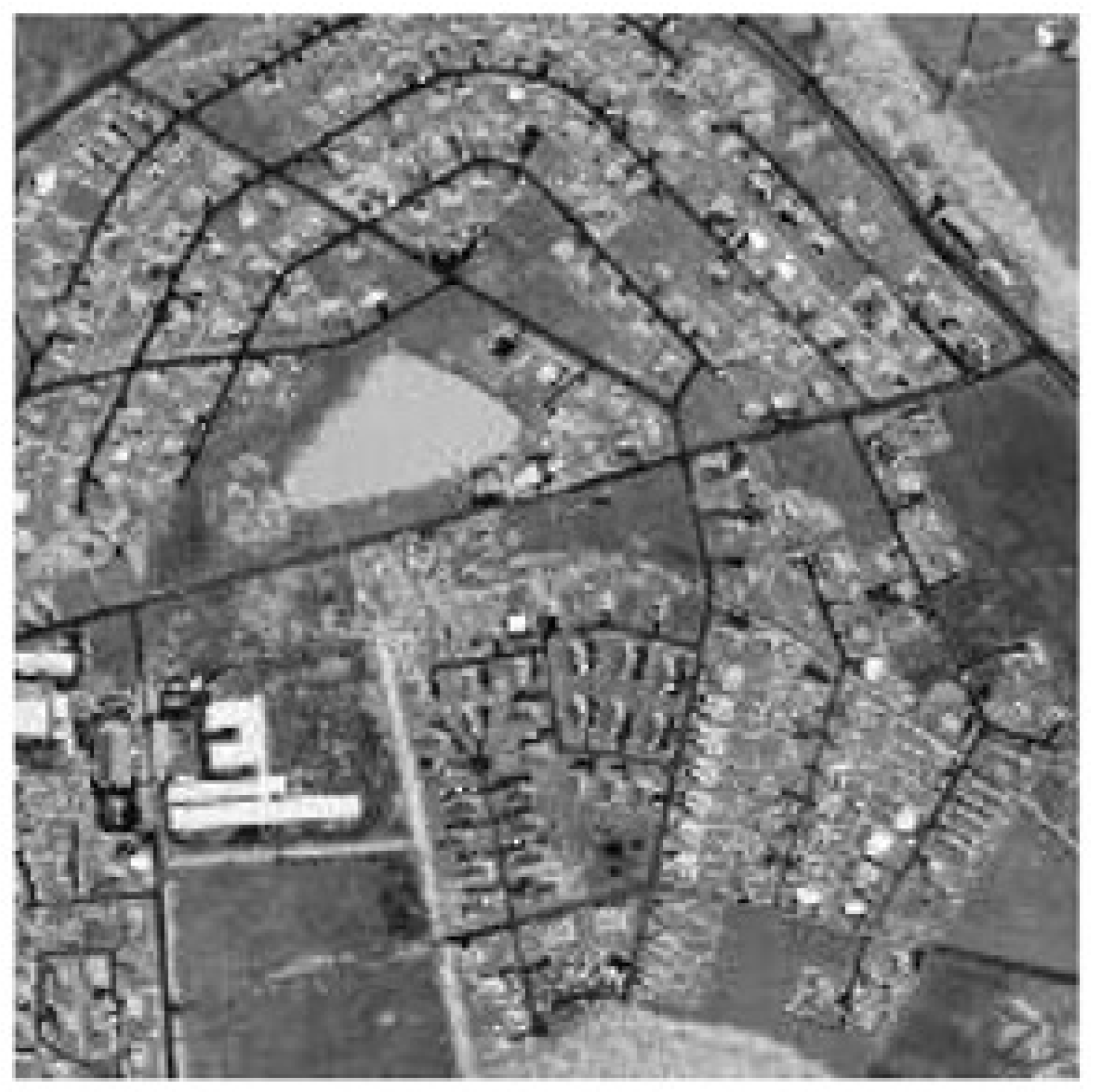
A CNN of three convolutional layers is trained with RGB images of 40 × 40 pixels, corresponding to a captured square area of five meters per side. The images for training and testing are included in the global image of Figure 7, a 1 km2 aerial capture of a region of Estonia, the same used in [41], with a resolution of 1/64 m2/pixel and available at https://geoportaal.maaamet.ee/eng/, accessed on 26 July 2023. We have divided the image into 25 regions of 200 m × 200 m each, then we have subdivided them into squares of 5 m × 5 m, that is to say, 40 × 40 pixels. For the training set, we have selected three of the 25 regions, so we have 4800 images, each labeled with a cost value between 0 and 1. Once the CNN is trained, the 40,000 images (40 × 40 pixels) in the 25 sectors of the global image are presented to the CNN to generate the terrain cost map.
Other authors have used the EKF to address this problem but in a different way. In [42], they use EKF in combination with particle filtering to trace roads in satellite images, starting from a specific point and direction. This method tends to recognize real roads due to the use of the gray level of the images to identify road profiles. In our article, we train a CNN with the FDEKF to generate a terrain traversability cost map, enabling the recognition of real paths and the planning of trajectories in other accessible areas based on the labels of the training data set.
First, the task has been faced as a regression problem; therefore, the output of the network is scalar. After has been approached as a classification problem, for which the output dimension of the network corresponds to the number of classes and the training set is relabeled by distributing the classes in equal intervals between 0 and 1.
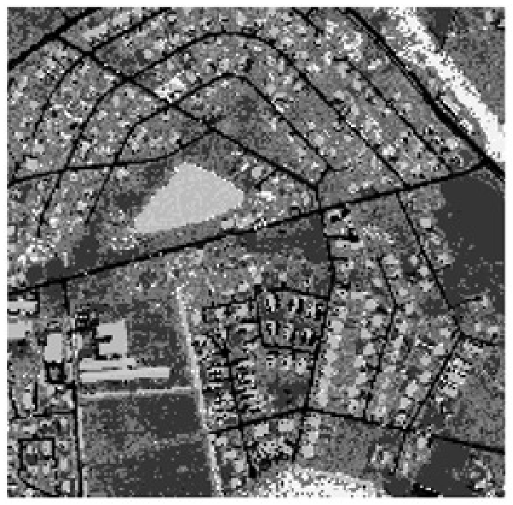
The result of the regression problem is interpreted through Figure 8, a grayscale image as a cost map. The traversability cost in the range [0, 1] of each 5 m × 5 m cell is directly represented by the pixel brightness. Therefore, the areas that are difficult to navigate are light, and the easier ones are dark. It is important to note that the simple grayscale image of the original image does not itself provide a cost map, making the objects reflect almost like easily traversable surfaces. The neural network learns features that determine the cost using different receptive fields, beyond the intensity of the individual pixel.
The cost map resulting from the CNN in the classification problem is shown in Figure 9. Compared to the image in the previous figure, this one has a higher contrast because the cost value is in a discrete range due to the choice of 20 classes in this experiment.
Both the continuous and discrete cost maps clearly show the surfaces that are easiest to navigate, and obviously, the roads of the urbanization are the darkest, then the small parking areas. Of the rest of the terrain, flat surfaces, without obstacles, with low grass appear less shiny. The results show significant generalization power: using only twelve percent of the total labeled terrain, the network learns to determine the traversability cost of any area of the terrain.

6. Conclusions

In this article, the FDEKF algorithm for training neural networks is applied in DCNNs for image classification, contrasting FDEKF with three other algorithms that have shown relevance in this type of task and of which two are very related to the FDEKF: Adam, which is a very popular first-order optimizer; sKAdam, which is based on Adam and EKF; and REKF, which has some similarities with FDEKF but is for minibatch training. The results are derived from experiments carried out with three data sets known in the field of image classification research, using DCNNs: fashion, sports and MNIST images.
The incorporation of second-order information from the FDEKF in the training results in faster learning concerning the number of samples presented and higher accuracy in the early stages, compared to the best first-order algorithms in the training of DCNNs for image classification. Although REKF also incorporates second-order information, its precision is not as high as that of FDEKF due to its way of applying the EKF to mini-batch training without respecting the recursion inherent to the EKF.
The FDEKF algorithm demonstrates superiority over other algorithms, more notable if the classification task is challenging. This was proved in an experiment with scenic, outdoor, and natural environment images of very low spatial resolution, which is even a challenge for human recognition.
In the application of the algorithm in the terrain recognition task to generate a cost map useful in the trajectory planning problem for autonomous navigation, the neural network learns characteristics beyond local information and simple color filtering.
On the other hand, sKAdam is notably more accurate than Adam in recognizing handwritten digit tasks. Being the sKAdam a procedure that adds to the original Adam the use of the EKF, in a completely scalar modality for the filtering of gradients.
As a future work, it will be interesting to test the FDEKF for different problems in which neural networks currently do not reach high precision. Also, applying the FDEKF to other models of DCNNs, such as ResNet-50, VGG-16, VGG-19, AlexNet, Inception-v3, and ResNet-50, is the next challenge. In addition to implementing the FDEKF for batch training and the EKF with another level of decoupling, such as the NDEKF.

Author Contributions

Conceptualization, A.G., O.B.-M. and N.A.-D.; Methodology, A.G., O.B.-M. and N.A.-D.; Software, A.G.; Validation, A.G., O.B.-M. and N.A.-D.; Formal analysis, A.G., O.B.-M. and N.A.-D.; Investigation, A.G., O.B.-M. and N.A.-D.; Resources, A.G., O.B.-M. and N.A.-D.; Data curation, A.G.; Writing – original draft, A.G., O.B.-M. and N.A.-D.; Writing – review and editing, A.G. and O.B.-M.; Visualization, A.G., O.B.-M. and N.A.-D.; Supervision, O.B.-M. and N.A.-D.; Project administration, O.B.-M.; Funding acquisition, O.B.-M. All authors have read and agreed to the published version of the manuscript.

Funding

This research received no external funding.

Data Availability Statement

Acknowledgments

The authors would like to thank Cinvestav for its support for this publication.

Conflicts of Interest

The authors declare no conflicts of interest.

References

  1. Bosch, J.; Olsson, H.H.; Brine, B.; Crnkovic, I. AI Engineering: Realizing the potential of AI. IEEE Soft. 2022, 39, 23–27. [Google Scholar] [CrossRef]
  2. Mukhamediev, R.I.; Symagulov, A.; Kuchin, Y.; Yakunin, K.; Yelis, M. From classical machine learning to deep neural networks: A simplified scientometric review. Appl. Sci. 2021, 11, 5541. [Google Scholar] [CrossRef]
  3. Sharma, N.; Sharma, R.; Jindal, N. Machine learning and deep learning applications—A vision. Glob. Transitions Proc. 2021, 2, 24–28. [Google Scholar] [CrossRef]
  4. Cao, L. Deep learning applications. IEEE Intell. Syst. 2022, 37, 3–5. [Google Scholar] [CrossRef]
  5. Sultana, J.; Usha Rani, M.; Farquad, M.A.H. An extensive survey on some deep-learning applications. In Emerging Research in Data Engineering Systems and Computer Communication; Venkata Krishna, P., Obaidat, M., Eds.; Springer: Singapore, 2020; pp. 311–519. [Google Scholar] [CrossRef]
  6. Zhang, Q.; Yang, L.T.; Chen, Z.; Li, P. A survey on deep learning for big data. Inf. Fusion 2017, 42, 146–157. [Google Scholar] [CrossRef]
  7. Hinton, G.E.; Osindero, S.; Teh, Y. A fast learning algorithm for deep belief nets. Neural Comput. 2006, 18, 1527–1554. [Google Scholar] [CrossRef]
  8. Schmidhuber, J. Deep learning in neural networks: An overview. arXiv 2015, arXiv:1404.7828. [Google Scholar] [CrossRef]
  9. Deng, L.; Yu, D. Deep Learning: Methods and Applications. Found. Trends Signal Process. 2014, 7, 197–387. [Google Scholar] [CrossRef]
  10. Rawat, W.; Wang, Z. Deep convolutional neural networks for image classification: A comprehensive review. Neural Comput. 2017, 29, 2352–2449. [Google Scholar] [CrossRef]
  11. Puskorius, G.V.; Feldkamp, L.A. Decoupled extended Kalman filter training of feedforward layered networks. In Proceedings of the IJCNN-91-Seattle International Joint Conference on Neural Networks, Seattle, WA, USA, 8–12 July 1991. [Google Scholar] [CrossRef]
  12. Wan, E.A.; Nelson, A.T. Dual extended Kalman filter methods. In Kalman Filtering and Neural Networks; Haykin, S., Ed.; John Wiley & Sons, Inc.: New York, NY, USA, 2001; pp. 123–174. [Google Scholar] [CrossRef]
  13. Singhal, S.; Wu, L. Training multilayer perceptrons with the extended Kalman algorithm. In Advances in Neural Information Processing Systems 1; Touretzky, D., Ed.; Morgan Kaufmann Publishers Inc.: San Francisco, CA, USA, 1988; pp. 133–140. [Google Scholar]
  14. Shah, S.; Palmieri, F. MEKA-a fast, local algorithm for training feedforward neural networks. In Proceedings of the 1990 IJCNN International Joint Conference on Neural Networks, San Diego, CA, USA, 17–21 June 1990. [Google Scholar] [CrossRef]
  15. Puskorius, G.V.; Feldkamp, L.A. Parameter-based Kalman filter training: The theory and implementation. In Kalman Filtering and Neural Networks; Haykin, S., Ed.; John Wiley & Sons, Inc.: New York, NY, USA, 2001; pp. 23–68. [Google Scholar] [CrossRef]
  16. Gaytan, A.; Begovich, O.; Arana-Daniel, N. Node-Decoupled Extended Kalman Filter versus Adam Optimizer in Approximation of Functions with Multilayer Neural Networks. In Proceedings of the 2023 20th International Conference on Electrical Engineering, Computing Science and Automatic Control (CCE), Mexico City, Mexico, 25–27 October 2023. [Google Scholar] [CrossRef]
  17. Kingma, D.P.; Ba, J.L. Adam: A method for stochastic optimization. In Proceedings of the 3rd International Conference for Learning Representations, ICLR 2015, San Diego, CA, USA, 7–9 May 2015. [Google Scholar]
  18. Camacho, J.; Villaseñor, C.; Alanis, A.Y.; Lopez-Franco, C.; Arana-Daniel, N. sKAdam: An improved scalar extension of KAdam for function optimization. IEEE Intell. Data Anal. 2020, 24, 87–104. [Google Scholar] [CrossRef]
  19. Ismail, M.; Attari, M.; Habibi, S.; Ziada, S. Estimation theory and neural networks revisited: REFK and RSVSF as optimization for deep-learning. Neural Netw. 2018, 108, 509–526. [Google Scholar] [CrossRef]
  20. Heimes, F. Extended Kalman filter neural network training: Experimental results and algorithm improvements. In Proceedings of the SMC’98 Conference Proceedings. 1998 IEEE International Conference on Systems, Man, and Cybernetics, San Diego, CA, USA, 14 October 1998. [Google Scholar] [CrossRef]
  21. Vural, N.M.; Ergüt, S.; Kozart, S.S. An efficient and effective second-order training algorithm for LSTM-based adaptive learning. IEEE Trans. Signal Process. 2021, 69, 2541–2554. [Google Scholar] [CrossRef]
  22. Fukushima, K. Neocognitron: A self-organizing neural network model for a mechanism of pattern recognition unaffected by shift in position. Biol. Cybern. 1980, 36, 193–202. [Google Scholar] [CrossRef]
  23. Chen, L.; Li, S.; Bai, Q.; Ya, J.; Jiang, S.; Miao, Y. Review of Image Classification Algorithms Based on Convolutional Neural Networks. Remote Sens. 2021, 13, 4712. [Google Scholar] [CrossRef]
  24. LeCun, Y.; Boser, B.E.; Denke, J.S.; Howard, R.E.; Hubbard, W.E.; Jackel, L.D. Handwritten digit recognition with a back-propagation network. In Advances in Neural Information Processing Systems 2; Touretzky, D., Ed.; Morgan Kaufmann Publishers Inc.: San Francisco, CA, USA, 1990; pp. 396–404. [Google Scholar]
  25. LeCun, Y.; Bengio, Y.; Hinton, G. Deep learning. Nature 2015, 521, 436–444. [Google Scholar] [CrossRef]
  26. Krizhevsky, A.; Sutskever, I.; Hinton, G.E. ImageNet classification with deep convolutional neural networks. Commun. ACM 2017, 60, 84–90. [Google Scholar] [CrossRef]
  27. Bengio, Y.; LeCun, Y.; Hinton, G. Deep learning for AI. Commun. ACM 2021, 64, 58–65. [Google Scholar] [CrossRef]
  28. Galanis, N.-I.; Vafiadis, P.; Mirzaev, K.-G.; Papakostas, G.A. Convolutional Neural Networks: A Roundup and Benchmark of Their Pooling Layer Variants. Algorithms 2022, 15, 391. [Google Scholar] [CrossRef]
  29. Hinton, G. The forward-forward algorithm: Some preliminary investigations. arXiv 2022, arXiv:2212.13345. [Google Scholar]
  30. Lu, A.; Honarvar Shakibaei Asli, B. Seismic Image Identification and Detection Based on Tchebichef Moment Invariant. Electronics 2023, 12, 3692. [Google Scholar] [CrossRef]
  31. Chen, B.; Zhang, L.; Chen, H.; Liang, K.; Chen, X. A novel extended Kalman filter with support vector machine based method for the automatic diagnosis and segmentation of brain tumors. Comput. Methods Programs Biomed. 2021, 200, 105797. [Google Scholar] [CrossRef]
  32. Kalman, R.E. A new approach to linear filtering and prediction problems. Trans. ASME J. Basic Eng. 1960, 82, 35–45. [Google Scholar] [CrossRef]
  33. Smith, G.L.; Schmidt, S.F.; McGee, L.A. Application of Statistical Filter Theory to the Optimal Estimation of Position and Velocity on Board a Circumlunar Vehicle; Technical Report R-135; NASA: Moffet Field, CA, USA, 1962.
  34. Alsadi, N.; Gadsden, S.A.; Yawney, J. Intelligent estimation: A review of theory, applications, and recent advances. Digit. Signal Process. 2023, 135, 103966. [Google Scholar] [CrossRef]
  35. Ruck, D.W.; Rogers, S.K.; Kabrisky, M.; Maybeck, P.S.; Oxley, M.E. Comparative analysis of backpropagation and the extended Kalman filter for training multilayer perceptrons. IEEE Trans. Pattern Anal. Mach. Intell. 1992, 14, 686–691. [Google Scholar] [CrossRef]
  36. Chernodub, A.N. Training neural networks for classification using the extended Kalman filter: A Comparative Study. Opt. Mem. Neural Netw. 2014, 23, 96–103. [Google Scholar] [CrossRef]
  37. Pereira de Lima, D.; Viana Sanchez, R.F.; Pedrino, E.C. Neural network training using unscented and extended Kalman filter. Robot Autom. Eng. J. 2017, 1, 100–105. [Google Scholar] [CrossRef]
  38. Gomez-Avila, J.; Villaseñor, C.; Hernandez-Barragan, J.; Arana-Daniel, N.; Alanis, A.Y.; Lopez-Franco, C. Neural PD Controller for an Unmanned Aerial Vehicle Trained with Extended Kalman Filter. Algorithms 2020, 13, 40. [Google Scholar] [CrossRef]
  39. Dubey, S.R.; Chakraborty, S.; Roy, S.K.; Mukherjee, S.; Singh, S.K.; Chaudhuri, B.B. diffGrad: An optimization method for convolutional neural networks. IEEE Trans. Neural Netw. Learn. Syst. 2020, 31, 4500–4511. [Google Scholar] [CrossRef]
  40. LeCun, Y.; Bottou, L.; Bengio, Y.; Haffner, P. Gradient-based learning applied to document recognition. Proc. IEEE 1998, 86, 2278–2324. [Google Scholar] [CrossRef]
  41. Hudjakov, R.; Tamre, M. Orthophoto Classification for UGV Path Planning using Heterogeneous Computing. Int. J. Adv. Robot. Syst. 2013, 10, 268. [Google Scholar] [CrossRef]
  42. Movaghati, S.; Moghaddamjoo, A.; Tavakoli, A. Road Extraction From Satellite Images Using Particle Filtering and Extended Kalman Filtering. IEEE Trans. Geosci. Remote Sens. 2010, 48, 2807–2817. [Google Scholar] [CrossRef]
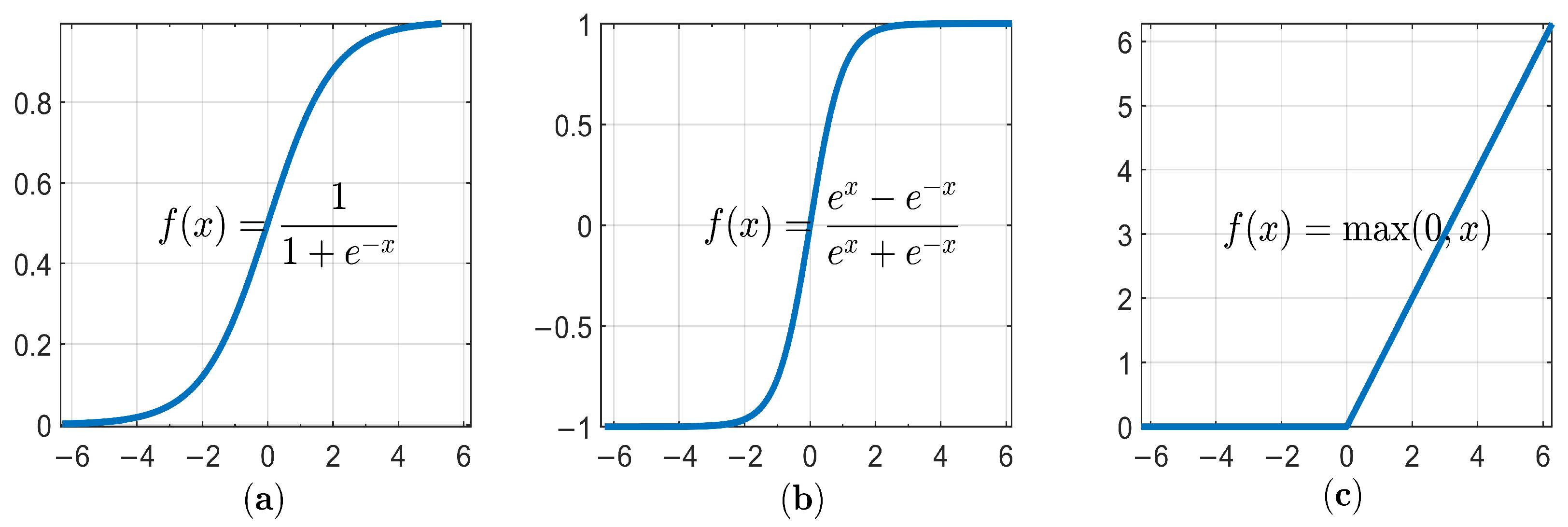
Figure 1. Activation functions: (a) logistic, (b) hyperbolic tangent, (c) ReLU.
Algorithms 17 00243 g001
Figure 2. Schematic illustration of the different levels of decoupling.
Algorithms 17 00243 g002
Figure 3. Fashion, Sports, and Handwritten Digits images.
Algorithms 17 00243 g003
Figure 4. FASHION with DCNN experiment—loss.
Algorithms 17 00243 g004
Figure 5. SPORTS with DCNN experiment—loss.
Algorithms 17 00243 g005
Figure 6. MNIST with DCNN experiment—loss.
Algorithms 17 00243 g006
Figure 7. Terrain image.
Algorithms 17 00243 g007
Figure 8. Cost map with DCNN in regression problem.
Algorithms 17 00243 g008
Figure 9. Cost map with DCNN in classification problem.
Algorithms 17 00243 g009
Table 1. Comparison of Accuracy and Standard Deviation for Fashion Test Set in Ten Training Process.
AlgorithmMean AccuracyStandard Deviation
Adam0.89010.0020
sKAdam0.89230.0021
REKF0.84330.0257
FDEKF0.90150.0025
Table 2. Comparison of Accuracy and SD for Sport Test Set after Ten Training Process.
AlgorithmMean AccuracyStandard Deviation
Adam0.91850.0073
sKAdam0.92090.0082
REKF0.86640.0092
FDEKF0.97890.0024
Table 3. Comparison of Accuracy and SD for MNIST Test Set after Ten Training Process.
AlgorithmMean AccuracyStandard Deviation
Adam0.8900 1.51 × 10 3
sKAdam0.9873 8.91 × 10 4
REKF0.9187 6.82 × 10 3
FDEKF0.9864 1.43 × 10 3
Disclaimer/Publisher’s Note: The statements, opinions and data contained in all publications are solely those of the individual author(s) and contributor(s) and not of MDPI and/or the editor(s). MDPI and/or the editor(s) disclaim responsibility for any injury to people or property resulting from any ideas, methods, instructions or products referred to in the content.