
Improved DQN for Dynamic Obstacle Avoidance and Ship Path Planning

Abstract
1. Introduction
2. Related Work
2.1. Ship Navigation Environment Modeling
2.2. Algorithm of Path Planning
3. The Proposed Deep Q Network(DQN)
3.1. The Original DQN
3.2. The Improved DQN
| Algorithm 1 DQN based on prioritized experience replay and multi-step updating |
Initialize Q and , let Q = , b, , ; for e = 1 to episodes repeat; Initialization status , perform action based on Q( -greedy strategy); obtain and the new state ; Store N samples (, , , ) to experience playback pool; Prioritized experience replay and multi-step update Q; Non-uniform sampling from experience playback pool with Equation (9); Calculate the target value with Equation (7); Update the parameters of so that Q is as close to y as possible; Reset Q = every m update; end for |
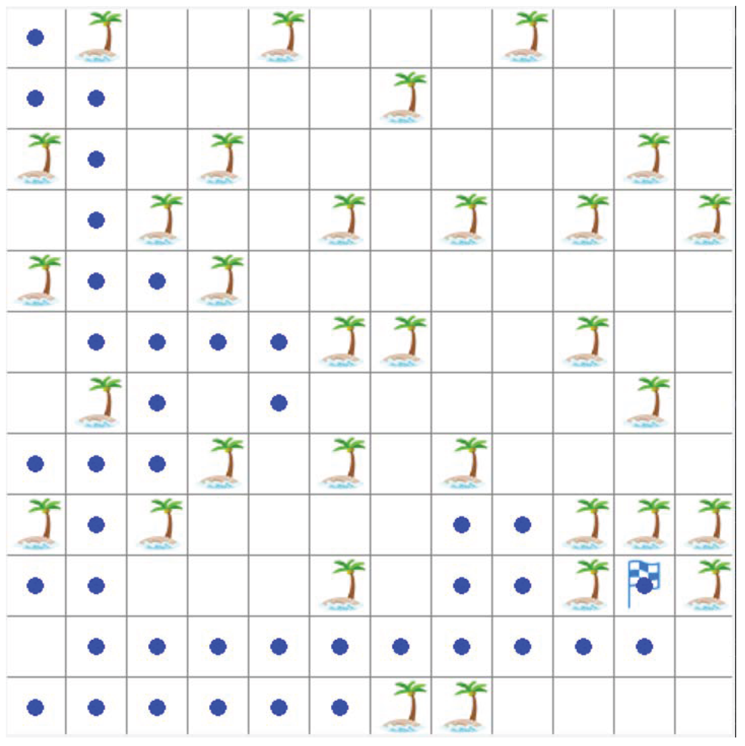
4. Experiment
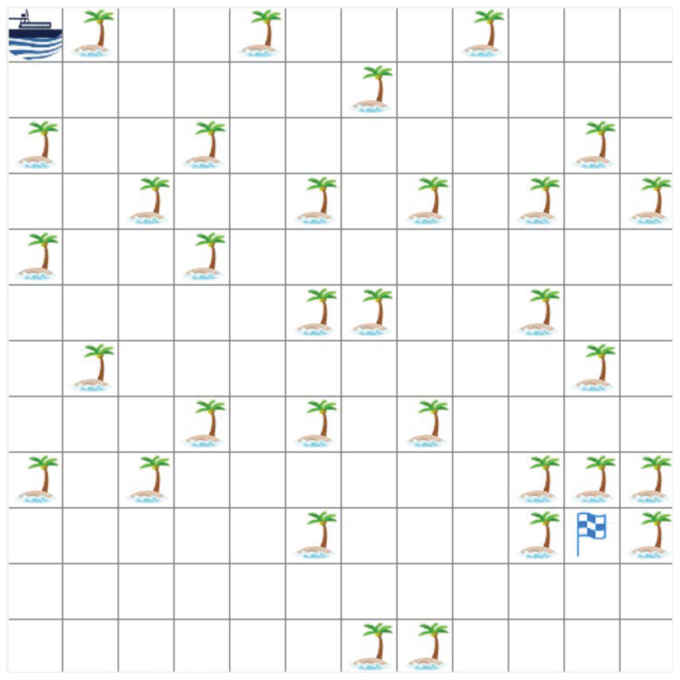
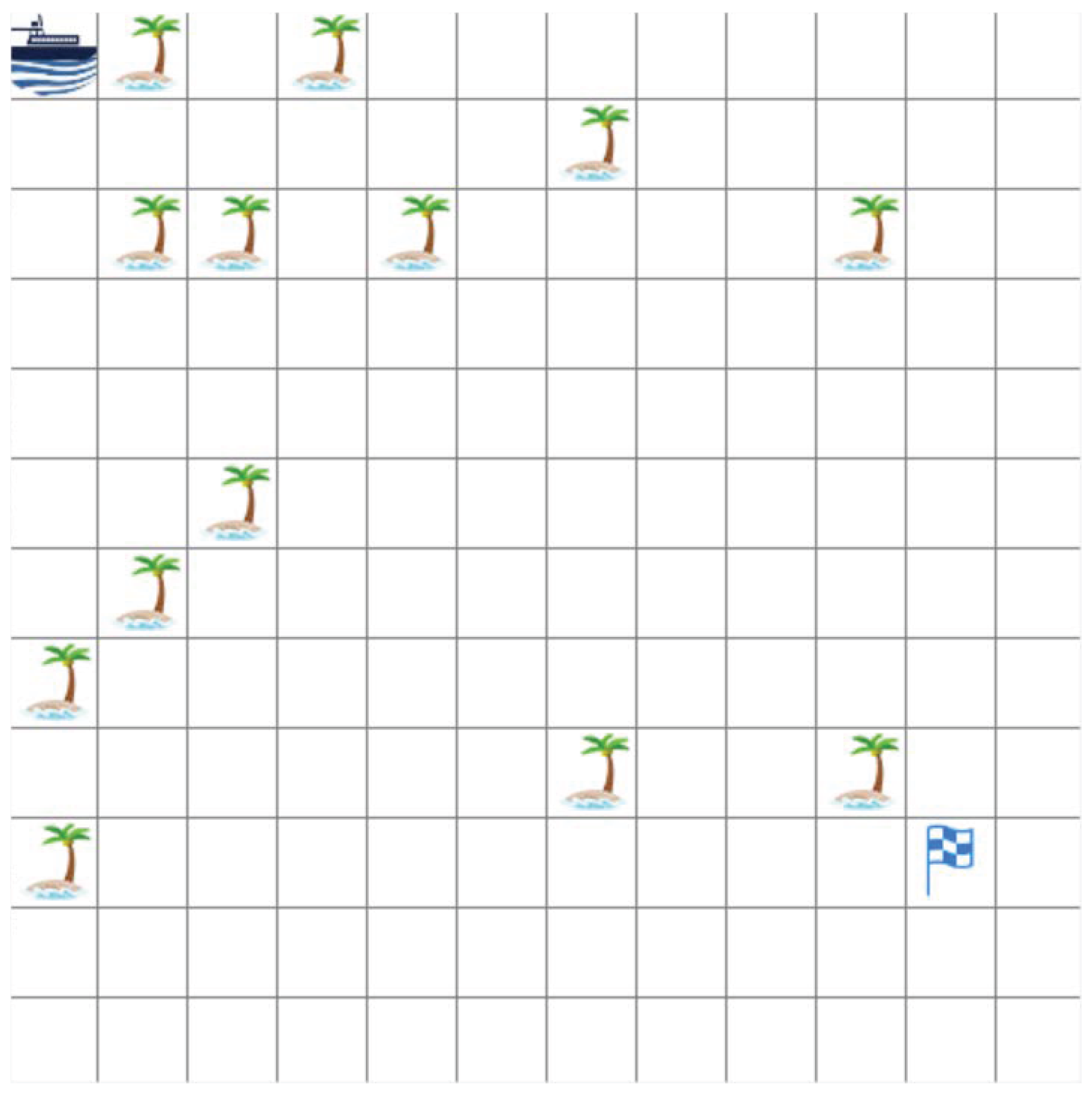
4.1. Environment and Parameter Settings
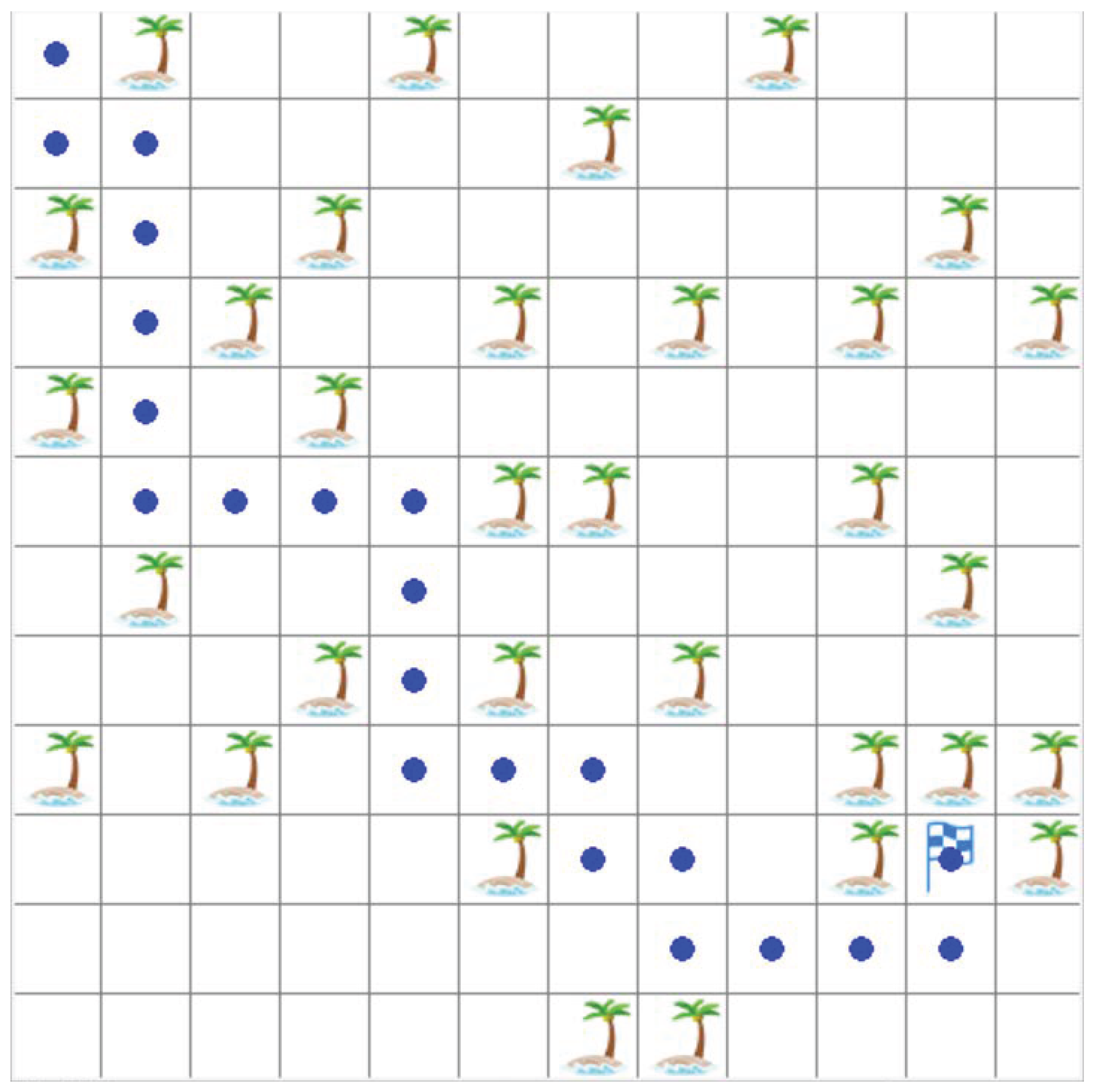
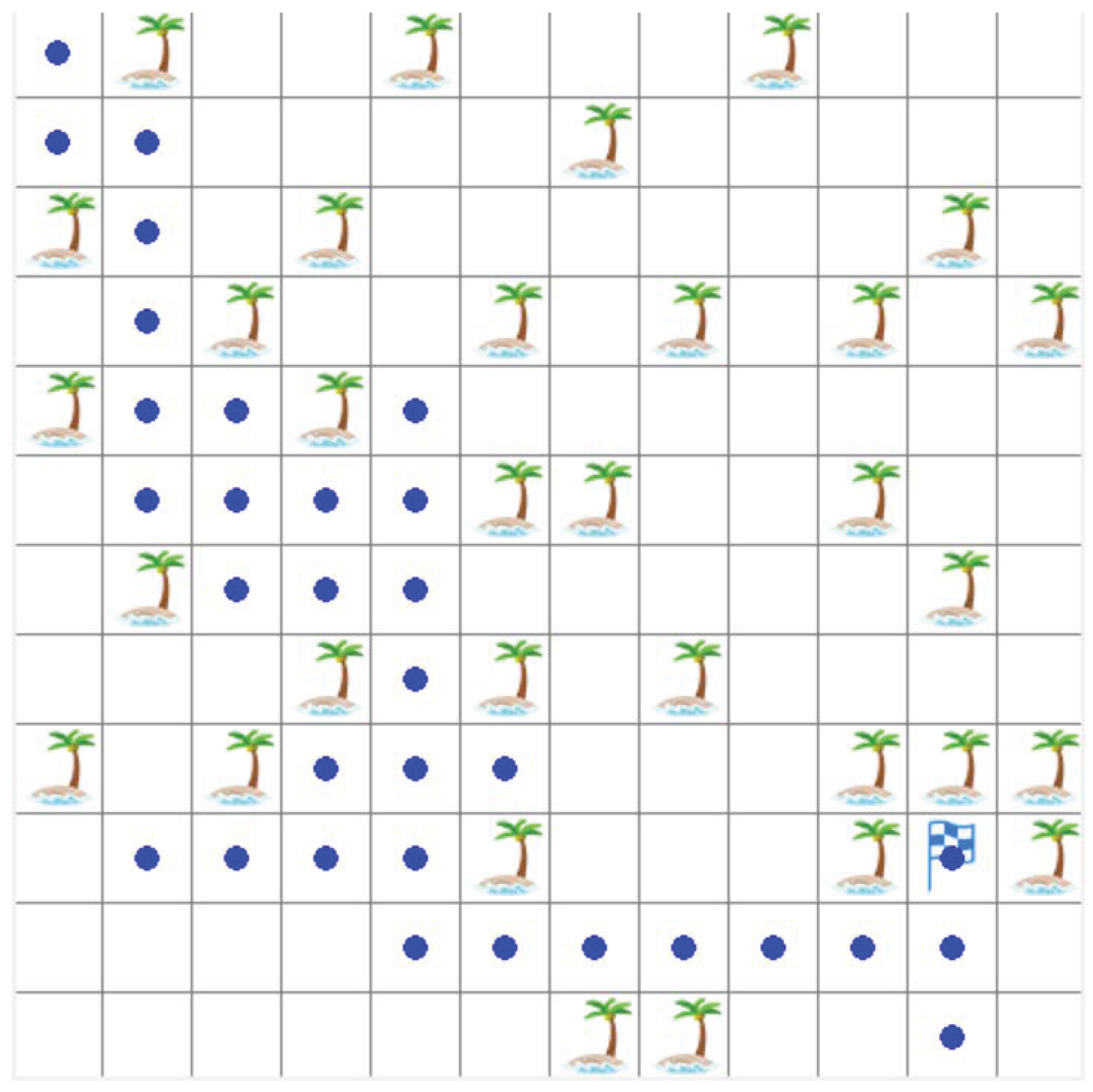
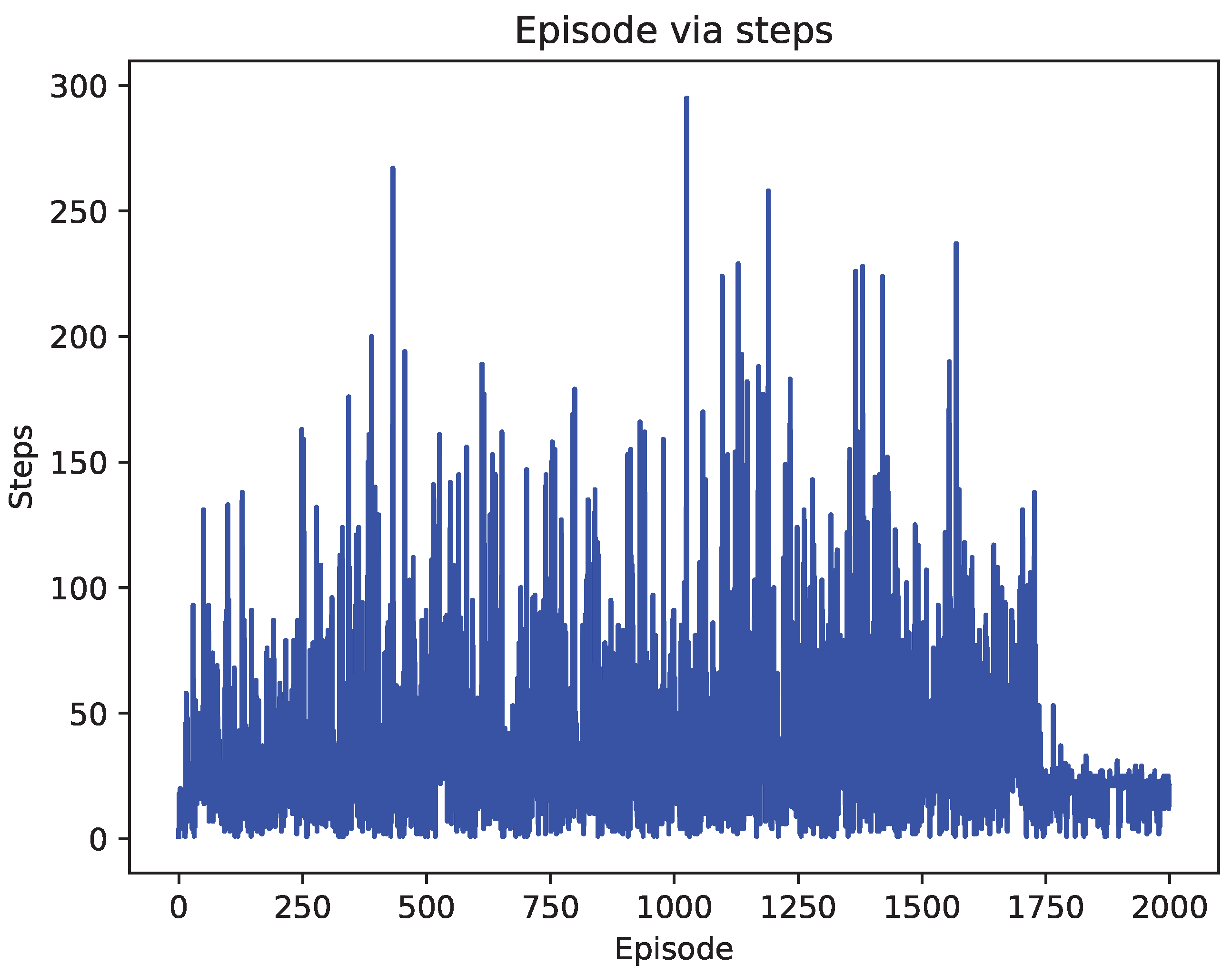
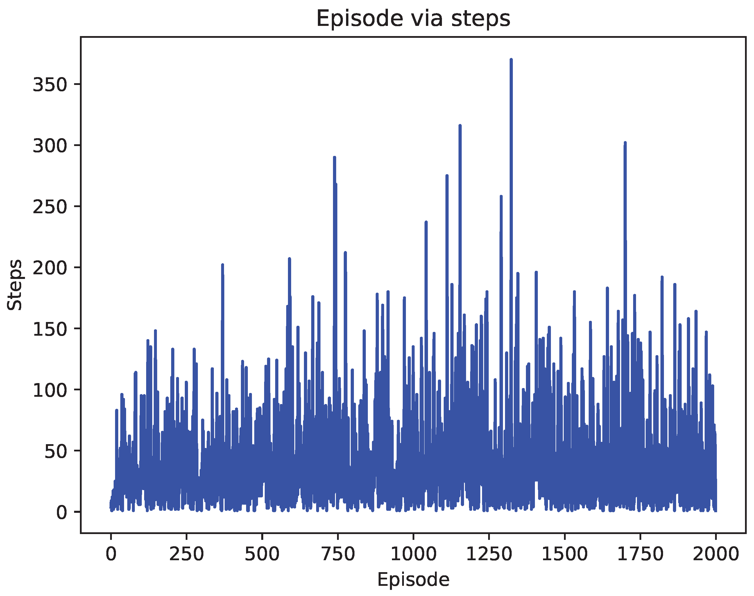
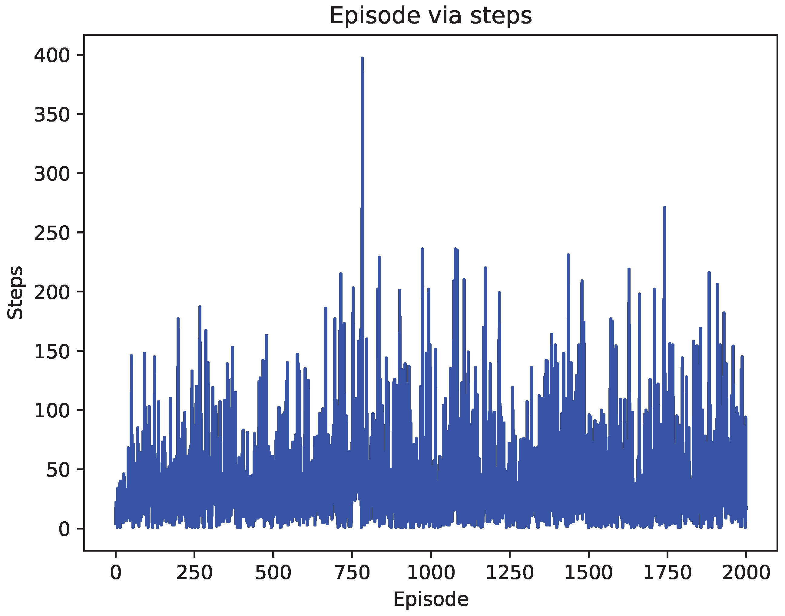
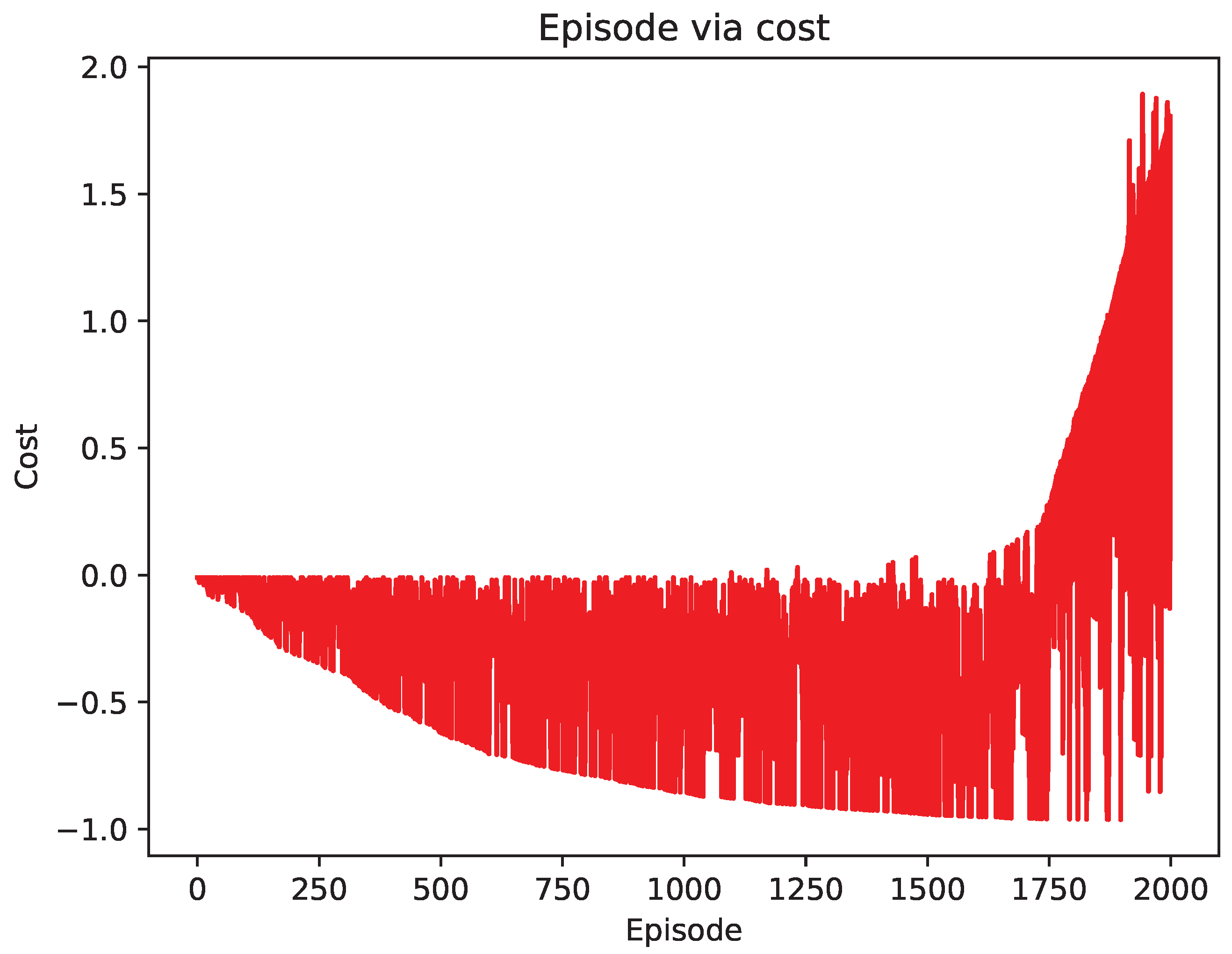
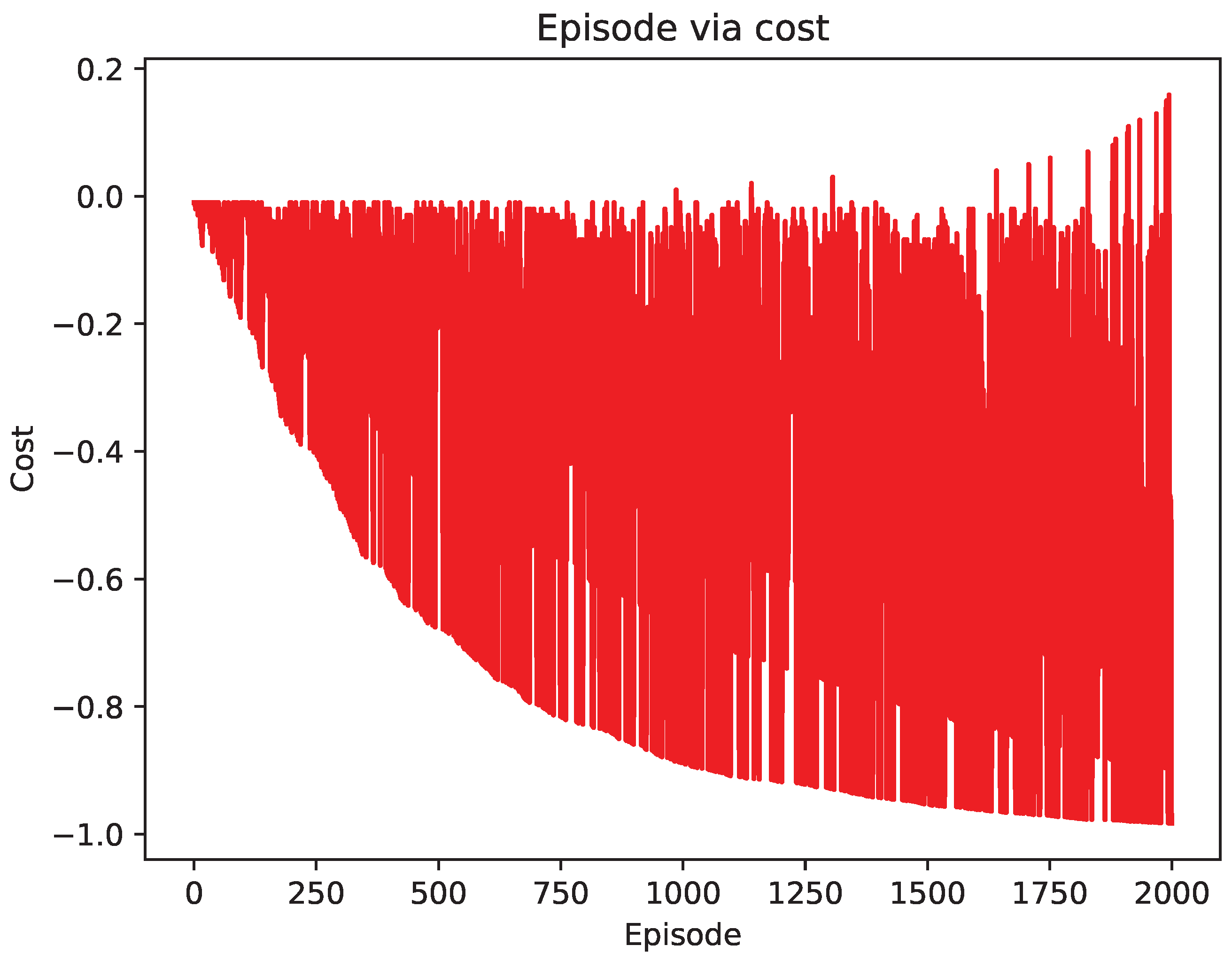
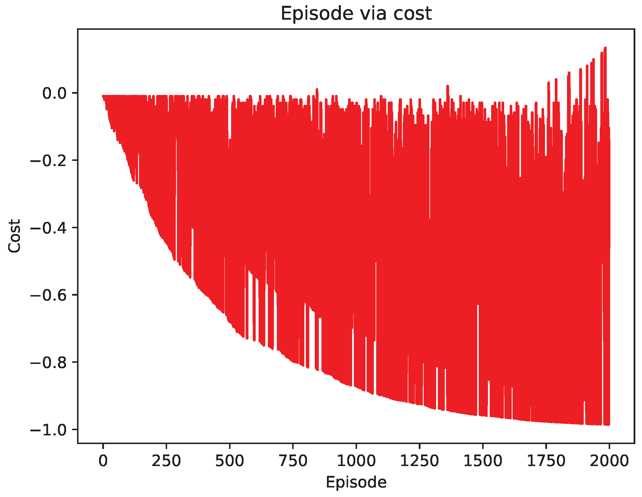
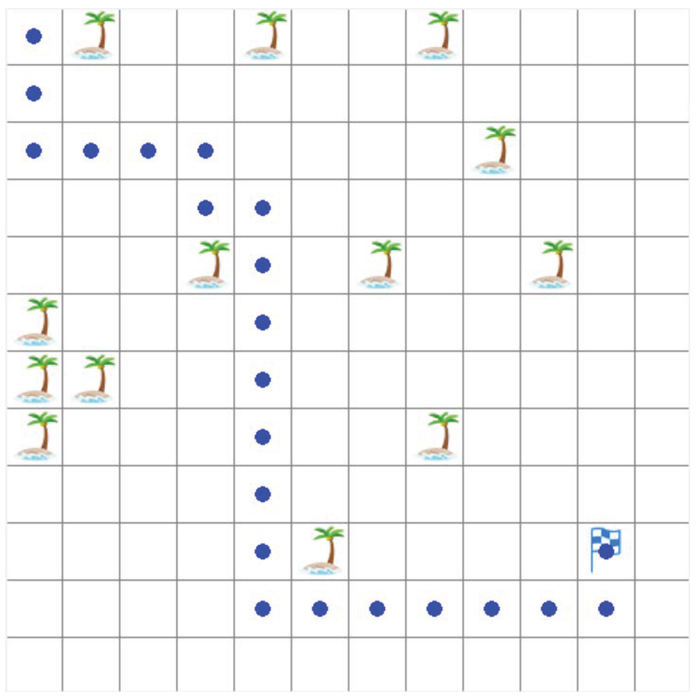
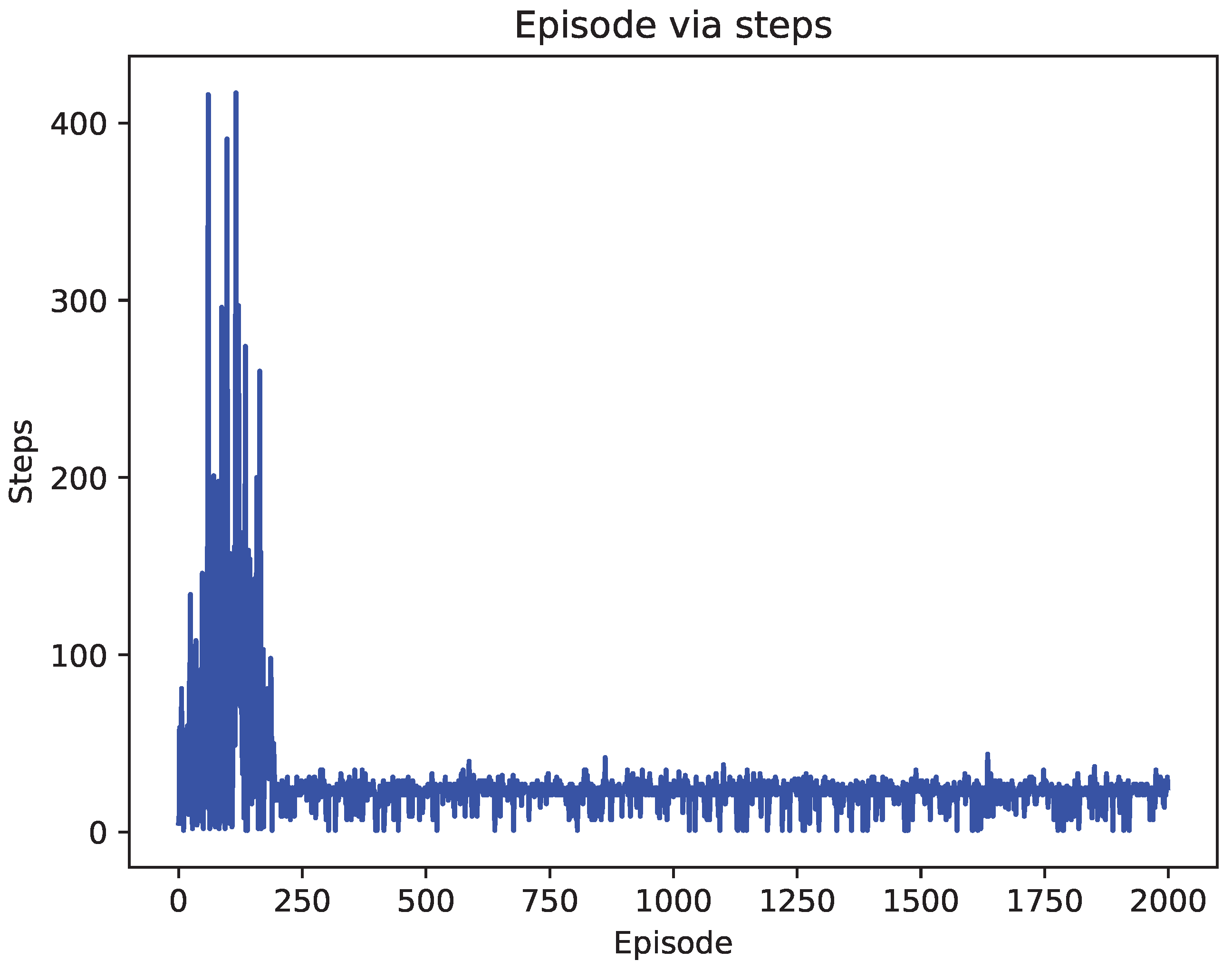
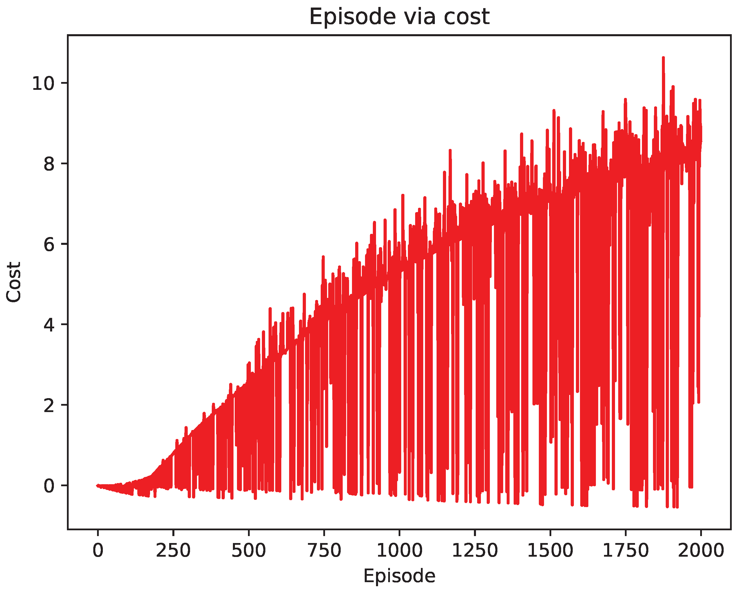
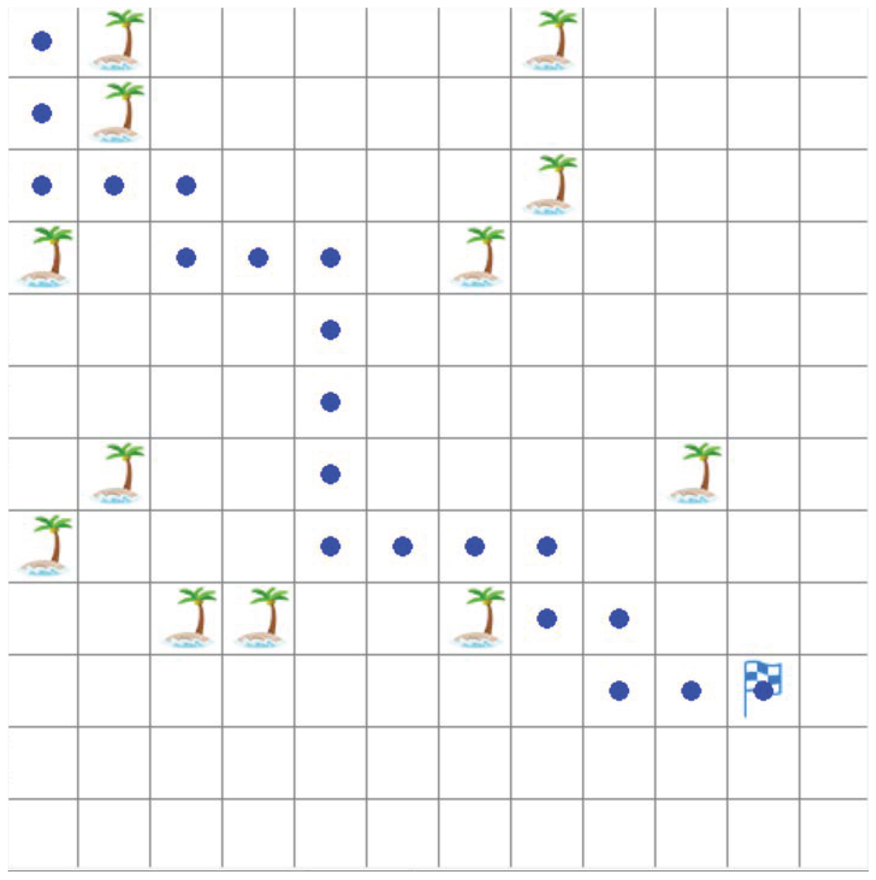
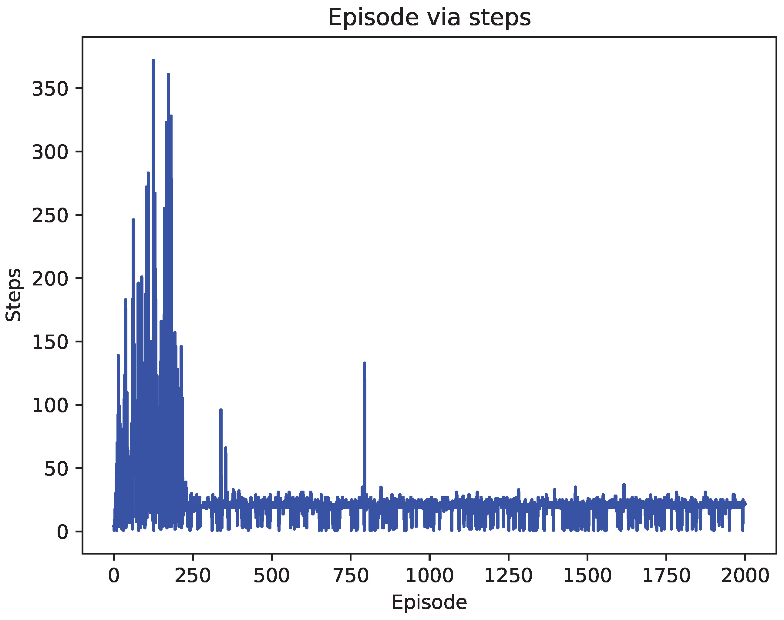
4.2. Comparison of Test Results
5. Discussion
Author Contributions
Funding
Institutional Review Board Statement
Informed Consent Statement
Data Availability Statement
Acknowledgments
Conflicts of Interest
References
- Zhang, X.; Wang, C.; Jiang, L.; An, L.; Yang, R. Collision-avoidance navigation systems for Maritime Autonomous Surface Ships: A state of the art survey. Ocean Eng. 2021, 235, 109380. [Google Scholar] [CrossRef]
- Jiang, L.; An, L.; Zhang, X.; Wang, C.; Wang, X. A human-like collision avoidance method for autonomous ship with attention-based deep reinforcement learning. Ocean Eng. 2022, 264, 112378. [Google Scholar] [CrossRef]
- Liu, Y.; Bucknall, R. Efficient multi-task allocation and path planning for unmanned surface vehicle in support of ocean operations. Neurocomputing 2018, 275, 1550–1566. [Google Scholar] [CrossRef]
- Wang, Z.; Xiang, X.; Yang, J.; Yang, S. Composite Astar and B-spline algorithm for path planning of autonomous underwater vehicle. In Proceedings of the 2017 IEEE 7th International Conference on Underwater System Technology: Theory and Applications (USYS), Kuala Lumpur, Malaysia, 18–20 December 2017; pp. 1–6. [Google Scholar]
- Zereik, E.; Sorbara, A.; Bibuli, M.; Bruzzone, G.; Caccia, M. Priority task approach for usvs’ path following missions with obstacle avoidance and speed regulation. IFAC-PapersOnLine 2015, 48, 25–30. [Google Scholar] [CrossRef]
- Chen, Z.; Yu, J.; Zhao, Z.; Wang, X.; Chen, Y. A Path-Planning Method Considering Environmental Disturbance Based on VPF-RRT. Drones 2023, 7, 145. [Google Scholar] [CrossRef]
- Szymak, P.; Praczyk, T. Using neural-evolutionary-fuzzy algorithm for anti-collision system of Unmanned Surface Vehicle. In Proceedings of the 2012 17th International Conference on Methods & Models in Automation & Robotics (MMAR), Miedzyzdroje, Poland, 27–30 August 2012; pp. 286–290. [Google Scholar]
- Chen, P.; Pei, J.; Lu, W.; Li, M. A deep reinforcement learning based method for real-time path planning and dynamic obstacle avoidance. Neurocomputing 2022, 497, 64–75. [Google Scholar] [CrossRef]
- Li, J.; Chen, Y.; Zhao, X.; Huang, J. An improved DQN path planning algorithm. J. Supercomput. 2022, 78, 616–639. [Google Scholar] [CrossRef]
- Xu, X.; Cai, P.; Ahmed, Z.; Yellapu, V.S.; Zhang, W. Path planning and dynamic collision avoidance algorithm under COLREGs via deep reinforcement learning. Neurocomputing 2022, 468, 181–197. [Google Scholar] [CrossRef]
- Xiaofei, Y.; Yilun, S.; Wei, L.; Hui, Y.; Weibo, Z.; Zhengrong, X. Global path planning algorithm based on double DQN for multi-tasks amphibious unmanned surface vehicle. Ocean Eng. 2022, 266, 112809. [Google Scholar] [CrossRef]
- Ru, J.; Yu, H.; Liu, H.; Liu, J.; Zhang, X.; Xu, H. A Bounded Near-Bottom Cruise Trajectory Planning Algorithm for Underwater Vehicles. J. Mar. Sci. Eng. 2022, 11, 7. [Google Scholar] [CrossRef]
- Saito, N.; Oda, T.; Hirata, A.; Nagai, Y.; Hirota, M.; Katayama, K.; Barolli, L. A Tabu list strategy based DQN for AAV mobility in indoor single-path environment: Implementation and performance evaluation. Internet Things 2021, 14, 100394. [Google Scholar] [CrossRef]
- Yang, Y.; Juntao, L.; Lingling, P. Multi-robot path planning based on a deep reinforcement learning DQN algorithm. CAAI Trans. Intell. Technol. 2020, 5, 177–183. [Google Scholar] [CrossRef]
- Yi, C.; Qi, M. Research on virtual path planning based on improved DQN. In Proceedings of the 2020 IEEE International Conference on Real-time Computing and Robotics (RCAR), Asahikawa, Japan, 28–29 September 2020; pp. 387–392. [Google Scholar]
- Bakdi, A.; Vanem, E. Fullest COLREGs evaluation using fuzzy logic for collaborative decision-making analysis of autonomous ships in complex situations. IEEE Trans. Intell. Transp. Syst. 2022, 23, 18433–18445. [Google Scholar] [CrossRef]
- Sang, H.; You, Y.; Sun, X.; Zhou, Y.; Liu, F. The hybrid path planning algorithm based on improved A* and artificial potential field for unmanned surface vehicle formations. Ocean Eng. 2021, 223, 108709. [Google Scholar] [CrossRef]
- Lyu, H.; Yin, Y. COLREGS-constrained real-time path planning for autonomous ships using modified artificial potential fields. J. Navig. 2019, 72, 588–608. [Google Scholar] [CrossRef]
- He, Z.; Liu, C.; Chu, X.; Negenborn, R.R.; Wu, Q. Dynamic anti-collision A-star algorithm for multi-ship encounter situations. Appl. Ocean Res. 2022, 118, 102995. [Google Scholar] [CrossRef]
- Zhou, S.; Wu, Z.; Ren, L. Ship Path Planning Based on Buoy Offset Historical Trajectory Data. J. Mar. Sci. Eng. 2022, 10, 674. [Google Scholar] [CrossRef]
- Bi, J.; Gao, M.; Zhang, W.; Zhang, X.; Bao, K.; Xin, Q. Research on Navigation Safety Evaluation of Coastal Waters Based on Dynamic Irregular Grid. J. Mar. Sci. Eng. 2022, 10, 733. [Google Scholar] [CrossRef]
- Yang, B.; Yan, J.; Cai, Z.; Ding, Z.; Li, D.; Cao, Y.; Guo, L. A novel heuristic emergency path planning method based on vector grid map. ISPRS Int. J. Geo-Inf. 2021, 10, 370. [Google Scholar] [CrossRef]
- Chen, J.; Bian, W.; Wan, Z.; Yang, Z.; Zheng, H.; Wang, P. Identifying factors influencing total-loss marine accidents in the world: Analysis and evaluation based on ship types and sea regions. Ocean Eng. 2019, 191, 106495. [Google Scholar] [CrossRef]
- Prpić-Oršić, J.; Vettor, R.; Faltinsen, O.M.; Guedes Soares, C. The influence of route choice and operating conditions on fuel consumption and CO2 emission of ships. J. Mar. Sci. Technol. 2016, 21, 434–457. [Google Scholar] [CrossRef]
- Harikumar, R.; Balakrishnan Nair, T.; Bhat, G.; Nayak, S.; Reddem, V.S.; Shenoi, S. Ship-mounted real-time surface observational system on board Indian vessels for validation and refinement of model forcing fields. J. Atmos. Ocean. Technol. 2013, 30, 626–637. [Google Scholar] [CrossRef]
- Zhen, Q.; Wan, L.; Li, Y.; Jiang, D. Formation control of a multi-AUVs system based on virtual structure and artificial potential field on SE (3). Ocean Eng. 2022, 253, 111148. [Google Scholar] [CrossRef]
- Shi, P.; Liu, Z.; Liu, G. Local Path Planning of Unmanned Vehicles Based on Improved RRT Algorithm. In Proceedings of the 2022 4th Asia Pacific Information Technology Conference, Bangkok, Thailand, 14–16 January 2022; pp. 231–239. [Google Scholar]
- Rudin, N.; Hoeller, D.; Reist, P.; Hutter, M. Learning to walk in minutes using massively parallel deep reinforcement learning. In Proceedings of the Conference on Robot Learning, PMLR, Auckland, NZ, USA, 14–18 December 2022; pp. 91–100. [Google Scholar]
- Chen, M.; Liu, W.; Wang, T.; Zhang, S.; Liu, A. A game-based deep reinforcement learning approach for energy-efficient computation in MEC systems. Knowl.-Based Syst. 2022, 235, 107660. [Google Scholar] [CrossRef]
- Boute, R.N.; Gijsbrechts, J.; Van Jaarsveld, W.; Vanvuchelen, N. Deep reinforcement learning for inventory control: A roadmap. Eur. J. Oper. Res. 2022, 298, 401–412. [Google Scholar] [CrossRef]
- Yuan, D.; Liu, Y.; Xu, Z.; Zhan, Y.; Chen, J.; Lukasiewicz, T. Painless and accurate medical image analysis using deep reinforcement learning with task-oriented homogenized automatic pre-processing. Comput. Biol. Med. 2023, 153, 106487. [Google Scholar] [CrossRef]
- Wang, C.; Zhang, X.; Yang, Z.; Bashir, M.; Lee, K. Collision avoidance for autonomous ship using deep reinforcement learning and prior-knowledge-based approximate representation. Front. Mar. Sci. 2023, 9, 1084763. [Google Scholar] [CrossRef]
- Zhai, P.; Zhang, Y.; Shaobo, W. Intelligent Ship Collision Avoidance Algorithm Based on DDQN with Prioritized Experience Replay under COLREGs. J. Mar. Sci. Eng. 2022, 10, 585. [Google Scholar] [CrossRef]
- Goswami, I.; Das, P.K.; Konar, A.; Janarthanan, R. Extended Q-learning algorithm for path-planning of a mobile robot. In Proceedings of the Simulated Evolution and Learning: 8th International Conference, SEAL 2010, Kanpur, India, 1–4 December 2010; Springer: Berlin/Heidelberg, Germany, 2010; pp. 379–383. [Google Scholar]
- Konar, A.; Chakraborty, I.G.; Singh, S.J.; Jain, L.C.; Nagar, A.K. A deterministic improved Q-learning for path planning of a mobile robot. IEEE Trans. Syst. Man Cybern. Syst. 2013, 43, 1141–1153. [Google Scholar] [CrossRef]
- Li, C.; Zheng, P.; Yin, Y.; Wang, B.; Wang, L. Deep reinforcement learning in smart manufacturing: A review and prospects. CIRP J. Manuf. Sci. Technol. 2023, 40, 75–101. [Google Scholar] [CrossRef]
- Song, D.; Gan, W.; Yao, P. Search and tracking strategy of autonomous surface underwater vehicle in oceanic eddies based on deep reinforcement learning. Appl. Soft Comput. 2023, 132, 109902. [Google Scholar] [CrossRef]
- Hu, H.; Yang, X.; Xiao, S.; Wang, F. Anti-conflict AGV path planning in automated container terminals based on multi-agent reinforcement learning. Int. J. Prod. Res. 2023, 61, 210. [Google Scholar] [CrossRef]
- Guo, S.; Zhang, X.; Du, Y.; Zheng, Y.; Cao, Z. Path planning of coastal ships based on optimized DQN reward function. J. Mar. Sci. Eng. 2021, 9, 210. [Google Scholar] [CrossRef]


| Configuration | Parameters |
|---|---|
| Operating system | CentOS Linux release 7.6.1810 (Core) |
| Memory | 754 G |
| CPU | Intel(R) Xeon(R) Platinum 8260 CPU |
| Basic frequency | 2.40 GHZ |
| Programing language | Python 3.8.3 |
| Graphics card | NVIDIA Corporation TU102GL (rev a1) |
| Algorithm | The Length of Path |
|---|---|
| The improved DQN | 21 |
| The original DQN | 32 |
| The Q-learning | 124 |
Disclaimer/Publisher’s Note: The statements, opinions and data contained in all publications are solely those of the individual author(s) and contributor(s) and not of MDPI and/or the editor(s). MDPI and/or the editor(s) disclaim responsibility for any injury to people or property resulting from any ideas, methods, instructions or products referred to in the content. |
© 2023 by the authors. Licensee MDPI, Basel, Switzerland. This article is an open access article distributed under the terms and conditions of the Creative Commons Attribution (CC BY) license (https://creativecommons.org/licenses/by/4.0/).
Share and Cite
Yang, X.; Han, Q. Improved DQN for Dynamic Obstacle Avoidance and Ship Path Planning. Algorithms 2023, 16, 220. https://doi.org/10.3390/a16050220
Yang X, Han Q. Improved DQN for Dynamic Obstacle Avoidance and Ship Path Planning. Algorithms. 2023; 16(5):220. https://doi.org/10.3390/a16050220
Chicago/Turabian StyleYang, Xiao, and Qilong Han. 2023. "Improved DQN for Dynamic Obstacle Avoidance and Ship Path Planning" Algorithms 16, no. 5: 220. https://doi.org/10.3390/a16050220
APA StyleYang, X., & Han, Q. (2023). Improved DQN for Dynamic Obstacle Avoidance and Ship Path Planning. Algorithms, 16(5), 220. https://doi.org/10.3390/a16050220