Abstract
This paper aimed to increase accuracy of an Alzheimer’s disease diagnosing function that was obtained in a previous study devoted to application of decision roots to the diagnosis of Alzheimer’s disease. The obtained decision root is a discrete switching function of several variables applicated to aggregation of a few indicators to one integrated assessment presents as a superposition of few functions of two variables. Magnetic susceptibility values of the basal veins and veins of the thalamus were used as indicators. Two categories of patients were used as function values. To increase accuracy, the idea of using artificial neural networks was suggested, but a feature of medical data is its limitation. Therefore, neural networks based on limited training datasets may be inefficient. The solution to this problem is proposed to preprocess initial datasets to determine the parameters of the neural networks based on decisions’ roots, because it is known that any can be represented in the incompletely connected neural network form with a cascade structure. There are no publicly available specialized software products allowing the user to set the complex structure of a neural network, which is why the number of synaptic coefficients of an incompletely connected neural network has been determined. This made it possible to predefine fully connected neural networks, comparable in terms of the number of unknown parameters. Acceptable accuracy was obtained in cases of one-layer and two-layer fully connected neural networks trained on limited training sets on an example of diagnosing Alzheimer’s disease. Thus, the scientific hypothesis on preprocessing initial datasets and neural network architecture selection using special methods and algorithms was confirmed.
1. Introduction
Data mining and machine learning methods are used in various areas including engineering, business and management, economics and finance, medicine, etc.
Artificial neural networks are actively used in the medical studies [1,2], etc., for example in diagnosing cardiovascular diseases [3,4,5], intestinal dysbacteriosis [6], oncology [7,8,9,10,11,12], in modeling of the prognosis of the outcome of the disease, and the likelihood of tumor recurrence [13,14,15]. In [16], it is proposed to use convolutional neural networks for automatic segmentation of edema in patients with an intracerebral hemorrhage. In [17], deep learning models are used to analyze the complication of cerebral edema induced by radiation therapy in patients with an intracranial tumor.
A feature of medical data is their limitation. This fact is partly due to ethical requirements, i.e., patients or their legal representatives must consent to the use of their medical data for scientific purposes and publication in open press. For example, researchers [18] took 5 years to collect data about 81 subjects, including 59 subjects with clinically diagnosed Alzheimer’s disease, and 22 elderly subjects did not have problems in cognitive abilities. This limited dataset was chosen for performance verification of neural network training after preprocessing initial datasets and neural network architecture selection using special methods and algorithms on an example of diagnosing Alzheimer’s disease. The key problem of Alzheimer’s disease is an accurate diagnosis in the early stages, where cognitive impairments do not yet appear at all or are not noticeable to the patient and others.
1.1. Related Papers
The key conclusions of some works of the last two decades [19,20,21,22] devoted to the study of the brain are the growth of diseases associated with Alzheimer’s disease, which does not immediately have distinctive signs for its identification. As shown in [23,24,25], there is a connection between oxygen saturation of brain tissues and the level of its blood circulation, qualitatively expressed through cerebral metabolism, with the symptoms of Alzheimer’s disease.
In [26], decrease of the dopaminergic activity of the ventral tegmental area (located in the midbrain area) may be of decisive importance for the earliest pathological symptoms of Alzheimer’s disease. This was verified by data analysis of resting structural and functional magnetic resonance imaging and neuropsychological assessments in 51 healthy adults. Mild cognitive impairments were diagnosed for 30 patients, and Alzheimer’s disease was diagnosed for 29 patients. A significant functional relationship was also noted between the ventral tegmental area and the hippocampus in pathological symptoms of Alzheimer’s disease. Changes in the dopaminergic system are often noted among patients with Alzheimer’s disease and are usually associated with cognitive and noncognitive symptoms [27].
In [28], it is shown that most dopamine-producing neurons are localized in the midbrain. Their loss is associated with some of the most famous human neurological disorders—Parkinson’s disease and cognitive impairments. In [29,30], the importance of dopamine is noted in participation in the mediated reaction of the body to the environment on different time scales (from fast impulse responses associated with rewards to slower changes with uncertainty, punishment, etc.). In [29], it is shown that the human brain contains about 200,000 dopamine neurons on each side of the brain. In [31,32,33], it is noted that cerebrovascular diseases largely stimulate the more rapid development of amnestic moderate cognitive impairments and Alzheimer’s disease and are also characterized by more severe damage to neuronal connections. In [34], the fact of increased cerebral blood flow without changing the oxygen consumption of the brain is described with the use of acetazolamide. This changes the signal observed on MRI images with a gradient echo from areas with increased cerebral blood flow. There is also a relationship between the oxygen content in the blood and the release of dopamine and neurotransmitters in [35,36]. In [37], the dependence of the level of dopamine and the oxygen content into the blood are noted. Since the neuron activity depends on the degree of oxygen uptake, the assessment of the degree of venous blood saturation can become an indicator of the functional state of neurons. Accordingly, we chose the following veins of all involved in the brain blood supply: the basal veins involved in the blood circulation of the striatum and veins of the thalamus (these veins drain the blood from the thalamus, which is closely connected with the midbrain [38]).
In [39], there is a fairly pronounced relationship between quantitative magnetic resonance imaging (MRI) and spectroscopy (MRS) measurements of energy metabolism (the rate of oxygen metabolism in the brain, CMR (O2)), the blood circulation (i.e., cerebral blood flow (CBF) and volume (CBV)) and functional MRI signal over a wide range of neuronal activity. Pharmacological treatments are used to interpret the neurophysiological basis of levels of the blood oxygenation dependent on image contrast at 7 T in glutamatergic neurons in the rat cerebral cortex.
1.2. Research Statement
The motivation for the present paper was continuation of the previous study [40] on the application of decisions’ roots to diagnosis of Alzheimer’s disease. “Decision root” is a new name for the integrated rating mechanisms traditionally applicated to aggregation of a few indicators into one integrated assessment [41]. The new term was proposed by Dr. Habil. Korgin, Nikolay A. and his Ph.D. student Sergeev, Vladimir A. [42] in November 2021. Previously, the term “integrated rating mechanisms” was used.
Historically, “the integrated rating mechanisms were introduced as multidimensional assessment and ranking systems for management and control in organizational and manufacturing systems in the Soviet Union in earlier 80th of the previous century” [43] (p. 610). Nowadays, these systems are used in different areas, including medicine [40]. Decision support system for diagnosis of Alzheimer’s disease is developed at the LLC “Diagnosing systems”.
Mathematically, the integrated rating mechanism is a discrete switching function of several variables presenting as a superposition of a few functions of two variables. Therefore, it can be represented in a hierarchical form, which determines the sequence of operations on variables. Each discrete function of two variables can be represented in matrix form. The tuple of criteria, binary trees and convolution matrices, located in its nodes, gives a graphical representation of such a function. In [44] (p. 1) it was said “integrated rating mechanism belongs to the class of so-called verbal decision analysis approaches”. Verbal decision analysis has been actively used for unstructured decision-making problems [45].
In 2020, two approaches to identification of integrated rating mechanisms based on a training set were suggested. The first one was proposed by Professor, Dr. Habil Burkov, Vladimir N., Dr. Habil Korgin, Nikolay A. and Sergeev, Vladimir A. [44]. This one-hot encoding approach considered the integrated rating mechanism as a sequence of matrix operations with one-hot encoded indicator values.
The second approach was proposed by one of the authors of this paper—Alekseev, Aleksandr O. and was based on truth table transformation [46], therefore, it was called the tabular algorithm for the identification of an integrated rating mechanism [47] (p. 599).
In 2021, Sergeev, Vladimir A. and Korgin, Nikolay A. [48] proposed to investigate the integrated rating mechanism identification problem on an incomplete dataset using equivalence groups. Approaches [46,47] and [48] are similar, but not the same.
In paper [46] (p. 402) it was shown that any integrated rating mechanism can be represented in the form of an artificial neural network. An identified neural network reproduces the training data with discrete values.
The obtained function, by using a tabular algorithm for identification [40], establishes the relationship between Alzheimer’s disease and the magnetic susceptibility value of the basal veins and veins of the thalamus. However, the accuracy of the function obtained in a previous study [40] was near 84%, which is not enough for its application in medical practice.
To increase accuracy, the idea was suggested to apply an artificial neural network to approximate the relationship between the magnetic susceptibility value of cerebral veins and Alzheimer’s disease. However, as previously mentioned, a feature of medical data is their limitation. In such cases, neural networks based on limited training datasets may be inefficient.
To solve this problem, it is proposed to preprocess initial datasets to determine the parameters of the neural networks based on the integrated rating mechanism (decision’s root). The scientific hypothesis of this paper is that it will be possible to obtain the acceptable accuracy of the neural network by training a neural network on the initial data in a continuous form.
Thus, the purpose of this work is performance verification of neural network training in cases of limited training sets on the example of diagnosing Alzheimer’s disease.
The paper is organized as follows: Section 2 provides initial data, methods and algorithms used in this study according to suggested methodology; Section 3 provides results of preliminary data analysis based on interval coding and identifies significant indicators of the study area. The architecture of the neural network based on the found decision’s root is proposed, which is the key result in this study, and the significance of the results is beyond doubt for development and discussion in future works; Section 4 is devoted to a discussion of the obtained results and the insights of this work. Lastly, the main results of this paper and future research directions are briefly discussed in Section 5.
2. Materials and Methods
2.1. Initial Data
In reference [49], it was shown that synthetic data can be used for neural network training, but in this paper, real medical data were taken for performance verification of neural network training based on preprocessing initial datasets and neural network architecture selection using special methods and algorithms.
The initial data were tomographic images of 81 patients examined using the mini-mental state examination (MMSE), Montreal cognitive assessment (MoCA), clock drawing task (CDT), and activity of daily living scale (ADL). Alzheimer’s disease was clinically diagnosed in 59 subjects (21 males and 38 females). These patients are hereinafter defined as in [18] as the AD group. Twenty-two patients (12 males, 10 females) did not have problems in cognitive abilities and were placed in the control group (defined as CON group).
The magnetic susceptibility values (MSV) of the following cerebral veins were quantified based on tomographic images: left and right basal veins (L_BV and R_BV, respectively), left and right internal cerebral veins (L_ICV, R_ICV), left and right veins of the thalamus (L_TV, R_TV), left and right septal veins (L_SV, R_SV), left and right veins of the dentate nucleus (L_DNV, R_DNV).
In this study, we exclusively used numerical data given in the appendix to the reference [18]. A fragment of the initial data is presented in Table 1.

Table 1.
The fragment of the initial data with magnetic susceptibility values of the cerebral veins [18].
2.2. Methodology and Methods
Data preprocessing consists in interval coding of initial data and search of integrated rating mechanisms (decisions’ roots). In paper [46] (p. 402), it is shown that any integrated rating mechanism can be represented in the form of an artificial neural network. Thus, it is possible to determine some of the parameters of the required neural network based on the integrated rating mechanism (decision’s root). This mechanism reproduces the encoded data using discrete values. This idea corresponds to the approach presented in reference [50]. The scientific hypothesis lies in the assumption that it will be possible to obtain the acceptable accuracy of the neural network by training a predefined neural network on the initial data in a continuous form.
According to [46] (p. 398) the integrated rating mechanism is determined as a tuple (1).
where G is a graph describing a sequence of convolution of particular criteria, M is a set of convolution matrices corresponding to the nodes of a criteria tree, X is a set of the scales for the scoring of the particular criteria, and P is the procedure of aggregation. In this study, discrete procedure is used, but continuous, interval, fuzzy and F–fuzzy procedures are also noted [51].
One of the problems of identifying integrated rating mechanisms (decisions’ roots) is the choice of the structure of the graph G, which is a full binary tree with labeled leaves [52], because their total number is determined according to the equation [43,48]:
where l is the total number of considered variables (leaves in terms of tree graph).
The number of G structures for 4 variables is 15, for 5–105, for 6–945 as can be seen from Equation (2), and there are already more than 34 million, for example, for 10 variables. This is a key limitation of the proposed algorithms, as can be seen from the above example.
To reduce the number of variables, it is suggested to use methods of the system-cognitive analysis (hereinafter–SCA) [53,54] using the computer program RU 2022615135 “Personal intelligent online development environment “EIDOS-X Professional” (System “EIDOS-Xpro”)” [55], developed by professor Lutsenko, Evgenue V. In this computer program, to solve the classification problem, two integrated similarity criteria are used, known as “Sum of knowledge” (3) and “Semantic resonance of knowledge” (4).
where —is the amount of information about class j; —the amount of features (signs, attributes); —a variable describing the presence () or absence () of the feature i; —assessment of informational importance of feature i for class j (amount of information about feature i for class j).
where —number of gradations of descriptive scales (features); —standard deviation particular criteria for class vector knowledge; —standard deviation along the vector of the recognized object; —average informativeness for class vector; —average for object vector.
In the case of diagnosing Alzheimer’s disease, index j is the ordinary number of patient group {group AD, group CON}, correspond to group AD, correspond to group CON. Index i is the ordinary number of the intervals of MSV of cerebral veins. We have 10 veins, each of which is divided into 3 equal intervals, so the total amount of MSV intervals is 30 (I = 30).
As a result of the implementation of the SC-analysis methods, the following model of determination informational importance (5) were selected as the most reliable.
where —the number of observations of the i-th feature (sign) for objects of the j-th class in the training sample; —the total number of observations of the i-th feature over the entire training sample; —the total number of features for objects of the j-th class in the training set; N—the volume of the training sample (number of observations).
These methods have been used to identify the most significant brain veins and subsequent reduction of the number of indicators.
The algorithm for identification of integrated rating mechanisms [47] has been used for data structuring and representation as a decision root. These algorithms were suggested previously by one of the authors of the present study–Alekseev, Aleksandr O.
A specialized computer program called “Neurosimulator 5.0” was used for neural network modeling [56]. It was developed by professor Yasnitsky, Leonid N. and his Ph.D student, Cherepanov, Fedor M.
For training the neural network, the computer program “Software package that implements the operation of incompletely connected neural networks” [57] was tested, but this program does not implement the conjugate gradient method. The application of this program is shown in the work [58].
Through inputs, the mathematical neuron receives input signals, which it sums up by multiplying each input signal by the appropriate weighting factor :
where Nn—the number inputs of i-th neuron; —signals on the input of the i-th neuron; —weights obtained in each iteration when performing neural network training.
Next, the activation function acts, which is usually an arbitrary monotonically increasing function that takes real values in the range from 0 to 1. The activation threshold is a number from the same interval.
where —output signal; —neural bias b is interpreted as the weight of an additional input with a synaptic link strength , whose signal x0 = 1; —activation function.
The general task of training a neural network is as follows:
Let X be a set of objects; R the solution of the algorithm, and then there is an unknown objective function . It is necessary to find such a primary function that restores the assessment . According to the generally accepted neural network design technology, the entire general population is divided into training, testing and confirming sets in the ratio of 70%: 20%: 10% [59].
Based on a set of logical pairs , where is n-th precedent, we will distinguish three relevant subsets of precedents —Train Set, —Test Set, —Validation Set, provided that data loss is excluded [60] (p. 426).
According to the methodology presented in Figure 1, the training of a non-fully connected neural network will be carried out by the method of conjugate gradients [61], which makes it possible to find the extrema of the function by iterative calculation. The conjugate gradient vector is determined by the following formula:
where the choice of the parameter responsible for the conjugate direction can be determined according to the Fletcher and Reeves algorithm [62] (10) or algorithm by Polak and Ribiere (11).
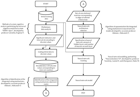
Figure 1.
Suggested algorithm of data preprocessing and neural network architecture selection for neural network training in limited initial dataset cases.
Two directions and are defined as conjugate if the following condition is met:
In other words, conjugate directions are orthogonal directions in the space of an identity Hessian matrix.
We chose the algorithm of elastic backpropagation (RPROP—Resilent back PROPagation) to train classic single-layer two-layer hidden artificial neural networks with a different number of neurons on each hidden layer. According to this algorithm, when correcting the weight coefficients, only the sign of the gradient matching [63]:
The methodology of this study is presented below (Figure 1).
3. Results
3.1. Results of the Preliminary Data Analysis
The initial data were processed using SCA methods. The intervals of magnetic susceptibility values of the above-described veins L_BV, R_BV, L_ICV, R_ICV, L_TV, R_TV, L_SV, R_SV, L_DNV, R_DNV were used as features. The state of the patient was used as a class: AD group or CON group, and the domains of observed values were divided into Three equal intervals for each vein (Table 2). Such a division of the initial dataset into three intervals was due to expert opinion, since when choosing two intervals, we get the classical problem of finding a Boolean function. The choice of four intervals is inappropriate, since when using 10 variables in the initial data, 80 features will be formed, and the initial dataset, which must be divided into training and testing, contains only 81 examples. Of interest is the division of the observation area into different intervals with an almost uniform number of examples in each of these intervals. In view of the multivariate results of possible partitions, this approach will be considered in a future study.

Table 2.
The intervals for discrete coding.
With the help of the intelligent analytical system “EIDOS-Xpro”, all patients were distributed based on the level of progression of Alzheimer’s disease by applying two integral similarity criteria: “Semantic resonance of knowledge” (4) and “Sum of knowledge” (3) (Figure 2).
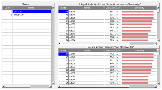
Figure 2.
Recognition results for the AD group of patients in the “Class-objects” mode in the system “EIDOS-Xpro”.
The intervals of MSV were determined as a result of the application of SCA. These values had the greatest informational significance for classification of a patient in the AD group (Figure 3, see “contributing”), as well as signs that did not characterize this class to the greatest extent (Figure 3, see “impending”). Since patients belong to only two classes (AD and CON) in the research dataset, the insignificance for the AD group meant significance for the CON group, respectively.
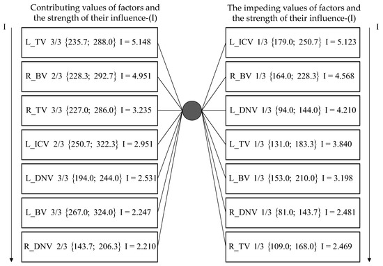
Figure 3.
The most significant factors influencing a possible brain pathology in the form of Alzheimer’s disease (after the name of the variable corresponding to a certain vein, the serial number of the interval of values out of 3 is indicated, and the interval of MSV values are directly indicated in curly brackets) [40] (p. 426).
It can be seen from the left part of Figure 3, that the 3rd interval of MSV in the veins of the thalamus (L_TV, R_TV) are among the first 3 most contributing factors, and the 1st interval of MSV in the same veins are impending factors (see right part of Figure 3). Second and third intervals of MSV for both the basal veins (R_BV, L_BV) were included in seven contributing factors for classification of a patient in the AD group (see Figure 3), and the first interval of MSV in both left and right basal veins are considered impending factors (see Figure 3) [40]. Thus, four indicators (L_BV, R_BV, L_TV, R_TV) were selected as the most significant from among all available indicators.
3.2. Results of Interval Coding Initial Data to Discrete Values
Veins of the thalamus L_TV, R_TV and in the basal veins L_BV, R_BV have intervals performed for coding to discrete values (see, Table 2).
The initial data were quantized by replacing the MSV values for a specific patient in a specific vein (L_BV, R_BV, L_TV, R_TV) with the value of the interval obtained using SCA methods after reducing the number of analyzed parameters. In other words, the original initial data set [18] was encoded (Table 3) to discrete values from one to three with correspondence to the number of MSV intervals (see, Table 2).

Table 3.
The fragment of the encoded data.
Subjects with the same vectors of encoded veins were united into 42 subgroups. For example, subjects 003 has a vector of values of the MSV {259.0; 172.0; 333.0; 159.0}, which was encoded to vector {2; 1; 3; 1}, and subjects 057 has a vector of values of the MSV {216.0; 147.0; 301.0; 140.0}, which was encoded to the same vector {2; 1; 3; 1}. Moreover, there were 8 contradictory examples in the encoded dataset. For example, from Table 3 we can see that subjects 001 and 079 have the same vector of discrete values {3; 1; 2; 1}, but they belong to different groups: AD and CON. To reduce conflict examples, we excluded those subgroups or subjects that had high level of similarity to one group but in fact belonged to another group. The similarity was measured in the System “EIDOS-Xpro” by values of the integrated similarity criteria using information model INF3.
The “EIDOS-Xpro” system, according to both integral similarity criteria “Semantic stability of knowledge” and “Sum of knowledge” with a value of 99.69% similarity, refers the patient sub007 to the CON groups, i.e., is not ill, while this patient is clinically diagnosed with Alzheimer’s disease (Figure 4).
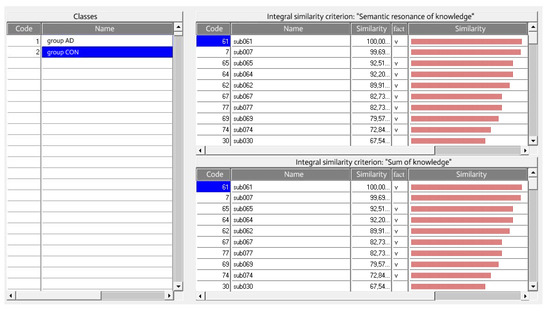
Figure 4.
Recognition results for CON group of patients in the “Class-objects” mode in the system “EIDOS-Xpro”.
Other subjects (Table 4) were excluded in the same way.

Table 4.
Subjects excluded from conflicting examples.
Subjects 057, 003, 076 and 075 were excluded from the encoded dataset because the vectors {2; 1; 3; 1}, {2; 2; 1; 3} corresponding to them have uncertainty.
The training set, after excluding the conflict examples, includes 34 unique, encoded vectors. They corresponded to 63 subjects (patients), which accounted for 78% of the original number of subjects. This training set for identification of the integrated rating mechanism (decision’s root) is presented in Table S1.
3.2.1. The Integrated Rating Mechanism (Decisions’ Roots) Identified Based on the Encoded Training Set
In the previous study [40], we used the identification algorithm proposed in [47], which is applicable to any structure of criteria trees without restrictions on the alphabet used inside the convolution matrix. Removing the restriction on the alphabet used to encode the elements of the convolution matrices, it is possible to approximate the initial data with several functions due to the fact that when gluing equivalence groups, the variability of these gluings arises [48].
As was said above, 15 full binary trees with named leaves are possible for 4 factors. From all possible tree structures in [40], it was proposed to convolve to produce indicators characterizing the left veins with each other, as well as the right ones with each other. This is because veins are paired and participate in the process of blood circulation of the two hemispheres separately and because arteries and veins in each of the hemispheres, and in the brain as a whole, have many collaterals that redistribute blood flow both among themselves at the beginning, within one hemisphere, and then, with a lack of compensatory capabilities within the entire brain (Figure 5).
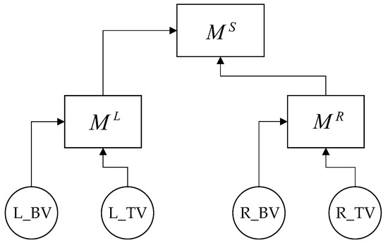
Figure 5.
Criteria tree structure of convolution for the basal and thalamic.
For each criteria tree structure, a few decisions’ roots can be identified; one example was presented in [40] (p. 426). The following decision’s root (Figure 5) was identified based in the training set presented in Table S2.
The founded decision root (see Figure 6) can be used to predefine architecture of the desired neural network.
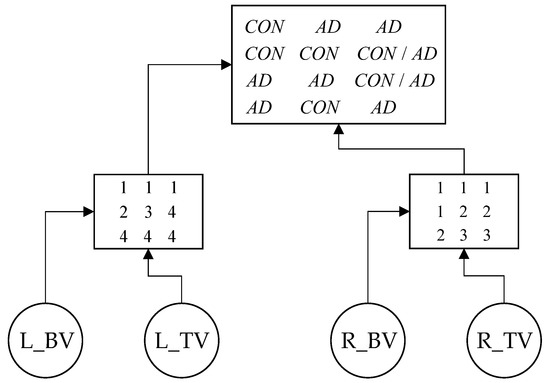
Figure 6.
Decision’s root for diagnosing Alzheimer’s disease. The values in the left matrix at the lower level are the average numbers of the rows of the root matrix, the values in the right matrix are the numbers of the columns of the root matrix, respectively.
3.2.2. Neural Network Architecture Selection
Using algorithm [47] (p. 402), we can predefine the neurons number of the desired neural network based on the decisions’ root (see, Figure 6). The first hidden layer has 12 neurons, because four input variables are indicated on Set 3 by encoded discrete values {1; 2; 3}. For both convolution matrices from the bottom level of the decisions’ roots, there are nine neurons on the second hidden layer, because matrices have nine elements. Matrix ML has four values, MR has three values, so the third hidden layer has seven neurons. The fourth hidden layer has 12 neurons because root matrix ML has 12 elements. The fifth hidden layer has two neurons because root matrix MS has values from set {CON; AD}. Thus, we have obtained a neural network with five hidden layers and 56 neurons on all layers (including one input and one output layer). The neural network architecture is shown in Figure 7, and the parameters of this network are presented in Table 5.
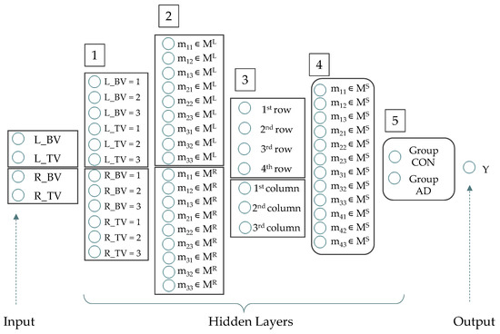
Figure 7.
Neurons of artificial neural network (where: vector of neurons on the Input Layer ∊ R4, vector of neurons on the Hidden Layer (1) ∊ R12, vector of neurons on the Hidden Layer (2) ∊ R18, vector of neurons on the Hidden Layer (3) ∊ R7, vector of neurons on the Hidden Layer (4) ∊ R12, vector of neurons on the Hidden Layer (5) ∊ R2, vector of neurons on the Output Layer ∊ R1).

Table 5.
Numbers of neurons in hidden layers of the desired artificial neural network.
The synaptic connections (Figure 8) are determined in full accordance with the elements of convolutional matrices in the decisions’ roots (see, Figure 6).
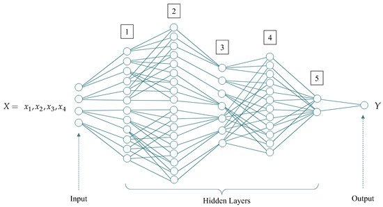
Figure 8.
Incompletely connected artificial neural network identified based on the decision root. Numbers from 1 to 5 designations of serial numbers of hidden layers of the neural network.
The total number of unknown parameters (synaptic coefficients) of the incompletely connected neural network predefined, based on the decision’s root is 158.
The structure of the predefined neural network model had 12 connections between the input signals and the first hidden layer (each connection generates two parameters of the mathematical model, which means that we have 24 parameters in total).
The next layer, in which the neurons correspond to the elements of the matrix, has three parameters each (two inputs from the previous layer and one unknown constant). Since we have two matrices of nine elements each at the bottom level of the criteria tree, this generates 18 neurons on the second layer, which means a total of 54 unknown parameters.
The next layer consists of the neurons corresponding to the matrix estimates, and there are exactly as many connections as there were neurons on the previous layer, i.e., in our case, 18, but we need to add seven parameters to them (determined by the number of neurons on the 3rd layer), which also means we have eighteen and seven parameters (25 parameters on the third layer).
Then, there is a matrix containing 12 elements, where each element corresponds to three parameters (two inputs and one unknown constant). It means 36 parameters on the 4th layer.
There are two neurons on the last hidden layer, where 14 input signals (10 neurons on the previous layer have one signal and two neurons have two signals; the last ones correspond to elements in the root matrix with value CON/AD, see Figure 6) plus two unknown constants (the number of neurons on the current layer) are taken.
There is only one signal at the output. This signal is associated with the last two neurons. It means there are three parameters (two inputs plus one unknown constant).
Thus, the total number of unknown parameters is determined by the sum (24 + 54 + 25 + 36 + 16 + 3 = 158).
Nowadays, it is worth noting that there are no publicly available specialized software products allowing the user to set the neural network structure, for example, to load the adjacency matrix or the incidence matrix of the graph corresponding to the neural network architecture. We tried to use the computer program “Software package that implements the operation of incompletely connected neural networks” [57]. It implemented incompletely connected neural networks only for one hidden layer, but as you can see from Figure 8, the required neural network has incompletely connected neurons on each hidden layer. Thus, this program is not applicable for this case.
Though there are no publicly available specialized software products allowing the user to set the structure of the neural network, we can find fully connected neural networks comparable in terms of the number of unknown parameters and compare the effectiveness of diagnosing Alzheimer’s disease knowing the number of unknown parameters that will be determined in the process of training the neural network.
Therefore, a fully connected single-layer neural network (Figure 9) with four input signals and one output signal has the following rule—each neuron on the hidden layer corresponds to four input-unknown variables corresponding to the input signals and one unknown constant (i.e., unknown parameters); the output signal receives signals from x neurons at the input and has one unknown constant.
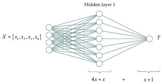
Figure 9.
Schematic representation of a single-layer neural network structure with x neurons and numbers of unknown parameters.
Thus, the number of unknown parameters in a fully connected network with one hidden layer can be expressed using the Equation (14)
According to (3), the minimum number of neurons on the hidden layer for a single-layer network is 27, where this number is comparable to the number of unknown parameters with the found incompletely connected neural network (see Figure 8).
The following equation will be obtained for a two-layer neural network structure (Figure 10):
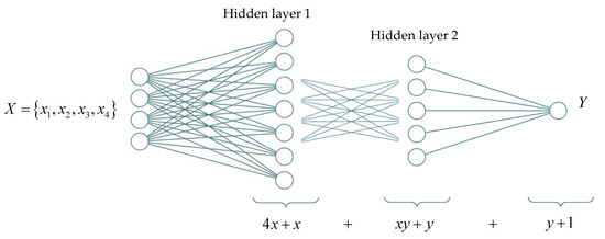
Figure 10.
Schematic representation of the structure of a fully connected two-layer neural network and the number of unknown parameters.
These minimal integer values x were found by changing the number of neurons on the second hidden layer y, starting from one, subject to the fulfillment of inequality (4). These values determine the number of neurons on the first hidden layer (Figure 11). Thus, various two-layer neural networks were found, where they are comparable in terms of the number of unknown neural network parameters (this network is built by the decision’s root) (see Figure 6).
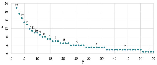
Figure 11.
The dependence of the number of neurons between the two layers (x—first hidden layer, y—second hidden layer).
3.2.3. Results of Neural Network Training
According to the generally accepted neural network design technology, the entire general population is divided into training, testing and confirming sets in the ratio of 70:20:10% [52]. In our problem, we neglect a strict formal approach to determining the percentage ratio between training, testing and confirming sets due to a fairly small number of examples, which is acceptable [63], thereby dividing the entire initial set only into training and testing in the ratio of 90:10%.
We performed multiple training and testing of neural networks for diagnosing Alzheimer’s disease on limited raw data using one-layer and two-layer neural networks. Several results of one-layer neural networks training and testing are shown below (Figure 12, Table 6).
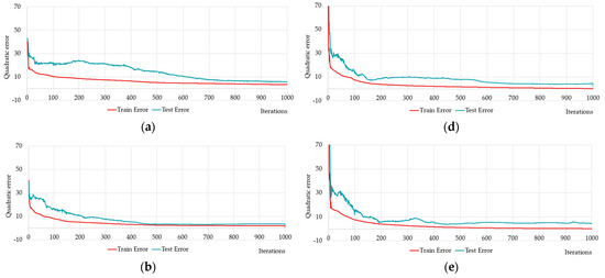

Figure 12.
Changing of the square errors at training and testing depending on iterations of calculation synaptic coefficients at fully connected one-layer neural networks with different numbers of neurons on the hidden layer (hereinafter the following designation will be used HL1 stands for neural network with 1 hidden layer): HL1-5 has 5 neurons (a); HL1-10 has 10 neurons (b); HL1-15 has 15 neurons (c); HL1-20 has 20 neurons (d), HL1-25 has 25 neurons (e), and fully connected one-layer neural network with predefined number of neurons HL1-27 has 27 neurons (f).

Table 6.
Results of a trained different fully connected one-layer neural networks.
Figure 12a–e shows five neural networks, distinguished by five neurons. Figure 12f shows the training and testing errors for the neural network HL1-27 with the 27 neurons satisfying inequality (14). Figure 12 shows that the quadratic error becomes less than 10% in all cases. Therefore, we should compare the results of the training with the other criteria: Q1–average quadratic relative (%); Q2–average relative error; Q3–average quadratic relative (Test, %); Q4–average relative error (Test); Q5–quadratic train error; Q6–quadratic test error; Q7–R2 train set; Q8–R2 test set (Table 6).
Comparing the performance by all the criteria in Table 6, it can be seen that the proposed neural network HL1-27 is better on almost all the criteria. At the same time, the best neural network training results from the multiple experiments we showed on both Figure 12a–e and the first seven rows of Table 6.
In our experiments, we noticed that the quality and speed of neural network learning could be improved by increasing the number of neurons. The neural network with predefined number of neurons HL1-27 (see Figure 12f) was trained rather quickly, and the results were more robust compared to variants HL1-5, HL1-10, HL1-15, HL1-20, which often over-trained the neural network.
We propose to consider nine variations of two-layer neural networks with different numbers of neurons on first and second hidden layers. The network structures are chosen so that the number of neurons on the first and the second hidden layer form a cross of gridlines with steps of five neurons—selected combinations of neuron number on the first and second layers are highlighted by black points (Figure 13, points 1–9).
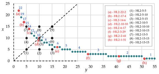
Figure 13.
Selected two-layers neural networks with different numbers of neurons on first and second hidden layers (hereinafter the following designation will be used–HL2 stands for two hidden layers, the next number after the hyphen stands for the number of neurons on the first hidden layer, and the last number stands for the number of neurons on the second hidden layer, respectively).
We also propose to consider several variations of neural networks whose structures are comparable to dependence (see, Figure 11). Selected eight combinations of neuron number on first and second are highlighted by red points (Figure 13, points a–h). This is necessary to assess the quality and ability to recognize and predict our neural network, the structure of which is determined according to the decision’s root and convolution matrices.
The dotted line in Figure 13 divides all neural networks into two types: in the upper left corner, there are neural networks with fewer neurons on the first layer than on the second layer. In the lower right area, on the contrary, there are neural networks with more neurons on the first layer than on the second layer.
The network HL2-10-10 refers to both a set of nine neural networks (see Figure 13, point 5) chosen by varying the number of variables on the first and second layer of five neurons (see Figure 13, black points 1–9), and a set of eight predefined neural networks (Figure 13, point d) that contain a number of synaptic coefficients comparable to a decision-root-based neural network (see Figure 8).
Therefore, out of nine neural networks, Figure 14 and Table 7 show the training and testing results of eight networks: HL2-5-5-5 (Figure 14a); HL2-5-10 (Figure 14b); HL2-5-15 (Figure 14c); HL2-10-5 (Figure 14d); HL2-10-15 (Figure 14e); HL2-15-5 (Figure 14f); HL2-15-10 (Figure 14g); and HL2-15-15 (Figure 14h).
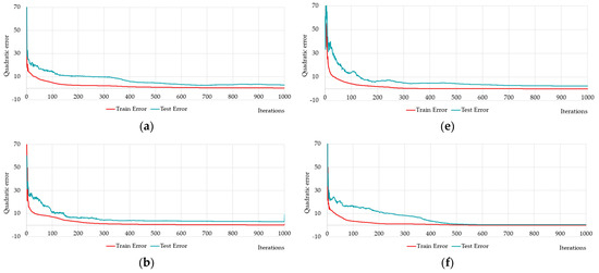
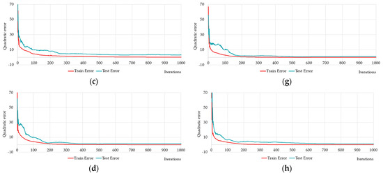
Figure 14.
Changing of the square errors at training and testing depending on iterations of calculation synaptic coefficients at two-layers neural networks with different numbers of neurons on the hidden layers: HL2-5-5 (a); HL2-5-10 (b); HL2-5-15 (c); HL2-10-5 (d); HL2-10-15 (e); HL2-15-5 (f); HL2-15-10 (g); HL2-15-15 (h).

Table 7.
Results of a trained different fully connected two-layer neural networks.
Figure 14 shows the networks HL2-10-5 (Figure 14d); HL2-15-5 (Figure 14f) and HL2-15-10 (Figure 14g) required fewer iterations to training.
Table 7 shows that the HL2-15-5 network is better than the others by all criteria except Q2–average relative error. The HL2-15-5 network is insignificantly inferior to the HL2-10-15 network in this criterion. At the same time, the HL2-10-15 network is inferior to other networks in many criteria.
It is of interest to compare the training results of randomly selected neural networks and predefined neural networks. Table 8 and Figure 15 show the results of training and testing of eight selected neural networks with predefined number of synaptic coefficients: HL2-22-2 (Figure 15a); HL2-17-4 (Figure 15b); HL2-14-6 (Figure 15c); HL2-10-10 (Figure 15d); HL2-6-17 (Figure 15e); HL2-3-29 (Figure 15f); HL2-2-41 (Figure 15g); HL2-1-51 (Figure 15h).

Table 8.
Results of a trained predefined fully connected two-layer neural networks.
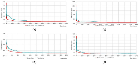
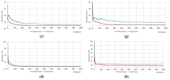
Figure 15.
Changing of the square errors at training and testing depending on iterations of calculation synaptic coefficients at two-layers neural networks with different numbers of neurons on the hidden layers: HL2-22-2 (a); HL2-17-14 (b); HL2-14-6 (c); HL2-10-10 (d); HL2-6-17 (e); HL2-3-29 (f); HL2-2-41 (g); HL2-1-51 (h).
The network HL2-15-5 is close to the predefined networks HL2-17-4 and HL2-14-6 by number of neurons, precisely these two networks with the HL2-10-10 network that have Q1 values less than one (see Table 8). The HL2-14-6 network has the lowest Q2, Q4 and Q5 values (see Table 8). HL2-10-10 has the lowest Q3, Q6 values (see Table 8). In terms of the coefficient of determination, the network HL2-14-6 has one, which means 100% of the variance of the resultant quantity in the training set is explained by the influence of selected variables.
Figure 15 shows that neural networks with a predefined number of neurons required significantly fewer iterations to train as compared to the brute-force selected networks. It is worth recalling again that Figure 14 and Figure 15 show the best results from the number of multiple computational experiments. A smaller number of iterations was required to train the predefined neural networks.
Having learnt the results of training two-layer networks, we noticed the following—the quality of neural network models is better if the number of neurons on the first layer is greater than on the second (Figure 14d–g and Figure 15a–d).
The results of training and testing two-layer neural networks are not entirely consistent with the observation in the case of single-layer neural networks. In the case of single layer neural networks, we observed the following—as the number of neurons on the hidden layer increases, the quality of neural network models becomes better. With two-layer networks, this is not true, e.g., HL2-22-2 with 24 neurons or HL2-17-4 with 21 neurons are in many ways (see Table 8) worse than the 20-neuron HL2-14-6 and HL2-10-10.
4. Discussion
Having compared all obtained results of training and testing of neural networks for diagnosing Alzheimer’s disease on limited data, it is possible to make a general conclusion—the constructed neural networks whose structure is chosen according to a predefined number of synaptic coefficients according to inequalities (14) and (15) have acceptable accuracy in comparison with neural networks whose structure is chosen by brute force.
In our experiments, we noticed that neural networks with a predefined number of neurons needed less training to obtain acceptable accuracy, and the results were more robust compared to neural networks with a random number of neurons. In the latter case, if the number of neurons was very different from the predefined number of neurons, we quite often observed retraining of neural networks.
The key value of the approach proposed in this paper for analyzing data and determining the structure of a neural network is to reduce the time spent on finding the optimal neural network, since based on the results of data preprocessing, we obtain an encoded data set, which is already a graph-matrix representation of the possible structure of the neural network. Moreover, the prospects for such an approach to data processing and analysis are reduced to improve the quality and accuracy of models on a limited data set, which we encountered in the study of brain disease in the form of Alzheimer’s disease.
Thus, it is possible to determine some of the parameters of the incomplete neural network with cascade structure based on the integrated rating mechanism (decision root). In future studies, we will use the term decisions-root-based neural network (DRB NN).
We would also like to point out that the best distribution for two-layer neural networks appears to be in the upper left corner of the space, separated by a dotted line (see Figure 13), which means that there should be fewer neurons on the first layer than on the second in the case of limited sets of training examples. Based on this, we can assume that in the case of multilayer neural networks, a similar ratio of neurons on upstream and downstream layers will also affect the quality of neural networks. This is fundamentally important for the proposed approach of building incomplete neural networks. Figure 8 clearly shows that the decisions-root-based neural network on layers three and five has a greater number of neurons than layers two and four, respectively. This could potentially limit the learning effectiveness of decision-root-based neural networks. However, the pattern described above regarding the correlation of neurons on previous and subsequent layers is true for fully connected neural networks. We will study incompletely connected neural networks in the future. This is of interest, and we plan to explore such a pattern in more detail in the following studies.
There are no publicly available specialized software products allowing the user to get the incompletely connected neural network structure. For example, the computer program “Software package that implements the operation of incompletely connected neural networks” [57] can create incompletely connected neural networks, but with only one hidden layer with incompletely connected neurons. It is not enough. Therefore, the authors intend to create a special computer program on software as a service available online for all researchers. This work is performed at the LLC “Perm Decision Making Support Center”.
5. Conclusions
It should be noted that the purpose of this study was achieved, and the hypothesis was confirmed. The neural network, preidentified, based on preprocessing initial datasets using suggested methods and algorithms, has acceptable accuracy in a case with a very limited training set. The suggested methodology consisting of interval coding of initial data and search of integrated rating mechanisms, following representation in the form of an artificial neural network and training using initial data, is effective.
Based on the results of this study, it should be noted that with the help of special methods based on the mechanism of complex assessment, it was possible to obtain the optimal structure of the neural network model capable of describing the study area with sufficient accuracy, using the example of Alzheimer’s disease. This, once again, confirms that neural network technologies are quite successful in medicine, which is especially valuable with a limited set of initial data. Similar conclusions about the successful application of neural network modeling in medicine and, in particular, the study of the brain, can be found in references [16,17] etc., where it was proposed to use convolutional neural networks and deep learning models in medicine.
Supplementary Materials
The following supporting information can be downloaded at: https://www.mdpi.com/article/10.3390/a16050219/s1, Table S1: The training set for identification of integrated rating mechanism (decisions’ root).
Author Contributions
Conceptualization, A.A. and L.K.; methodology, A.A.; software, L.K.; validation, A.A., L.K., V.N. and J.B.; formal analysis, A.A., L.K., V.N. and J.B.; investigation, A.A. and L.K.; resources, L.K.; data curation, A.A. and L.K.; writing—original draft preparation, A.A., L.K. and V.N.; writing—review and editing, A.A., L.K., V.N. and J.B.; visualization, L.K. and J.B.; supervision, A.A.; project administration, L.K.; funding acquisition, A.A. and L.K. All authors have read and agreed to the published version of the manuscript.
Funding
This research was carried out with the financial support of the Ministry of Science and Higher Education of the Russian Federation in the framework of the program of activities of the Perm Scientific and Educational Center “Rational Subsoil Use”.
Institutional Review Board Statement
Not applicable.
Informed Consent Statement
Not applicable.
Data Availability Statement
In this study, we used exclusively numerical data given in the appendix to the reference [18]. The computer programs we used by license CC BY-SA 4.0. The computer program RU 2022615135 “Personal intelligent online development environment “EIDOS-X Professional” (System “EIDOS-Xpro”)” [55] available at: http://lc.kubagro.ru/aidos/_Aidos-X.htm (accessed on 30 December 2022). The computer program RU 2014618208 “Neurosimulator 5.0” [56] available at: https://www.lbai.ru/#;show;install (accessed on 30 December 2022).
Acknowledgments
The authors are grateful to Valerii Yu. Stolbov from the Perm National Research Polytechnic University (Perm, Russia) for scientific supervising of the project ”New materials and technologies for medicine” at the Perm Scientific and Educational Center “Rational Subsoil Use”; Evgenue V. Lutsenko from the Kuban State Agrarian University (Krasnodar, Russia) for free access to the computer program “EIDOS-Xprofessional” [55]; Leonid N. Yasnitsky from the Perm State University (Perm, Russia) and Fedor M. Cherepanov from the Perm State Humanitarian Pedagogical University (Perm, Russia) for free access to the computer program “Neurosimulator 5.0” [56], and also to Nikolay A. Korgin from V.A. Trapeznikov Control Sciences Institute (Moscow, Russia), proposed term “decisions’ roots” [42], for statement of integrated rating mechanisms identification problem. We also sincerely thank all reviewers for their thoughtful comments and recommendations, especially, the first reviewer for suggesting the term “Decisions-Root-based Neural Network”, We will use such term in our future studies and papers.
Conflicts of Interest
The authors declare no conflict of interest.
References
- Yasnitsky, L.N.; Dumler, A.A.; Cherepanov, F.M.; Yasnitsky, V.L.; Uteva, N.A. Capabilities of neural network technologies for extracting new medical knowledge and enhancing precise decision making for patients. Expert Rev. Precis. Med. Drug Dev. 2022, 7, 70–78. [Google Scholar] [CrossRef]
- Yasnitsky, L.N. Artificial intelligence and medicine: History, current state, and forecasts for the future. Curr. Hypertens. Rev. 2020, 16, 210–215. [Google Scholar] [CrossRef] [PubMed]
- Pyatakovich, F.A.; Khlivnenko, L.V.; Mevsha, O.V.; Yakunchenko, T.I.; Makkonen, K.F. Development of a biotechnical system based on the functioning of neural networks for solving the problem of the scattergrams analysis. Netw. Electron. Sci. Educ. J. Mod. Issues Biomed. 2018, 3, 171–183. [Google Scholar]
- Bogdanov, L.A.; Komossky, E.A.; Voronkova, V.V.; Tolstosheev, D.E.; Martsenyuk, G.V.; Agienko, A.S.; Indukaeva, E.V.; Kutikhin, A.G.; Tsygankova, D.P. Prototyping neural networks to evaluate the risk of adverse cardiovascular outcomes in the population. Fundam. Clin. Med. 2021, 6, 67–81. [Google Scholar] [CrossRef]
- Kilic, A. Artificial Intelligence and Machine Learning in Cardiovascular Health Care. Ann. Thorac. Surg. 2020, 109, 1323–1329. [Google Scholar] [CrossRef]
- Solodukha, T.V. Development of a Specialized Computer System Based on Neural Networks for Predicting the Consequences of Allergic Reactions. Master’s Thesis, Donetsk National Technical University, Donetsk, Ukraine, 2002. [Google Scholar]
- Carrara, M.; Bono, A.; Bartoli, C.; Colombo, A.; Lualdi, M.; Moglia, D.; Santoro, N.; Tolomio, E.; Tomatis, S.; Tragni, G.; et al. Multispectral imaging and artificial neural network: Mimicking the management decision of the clinician facing pigmented skin lesions. Phys. Med. Biol. 2007, 52, 2599–2613. [Google Scholar] [CrossRef] [PubMed]
- Gruvberger-Saal, S.K.; Edén, P.; Ringnér, M.; Baldetorp, B.; Chebil, G.; Borg, A.; Fernö, M.; Peterson, C.; Meltzer, P.S. Predicting continuous values of prognostic markers in breast cancer from microarray gene expression profiles. Mol. Cancer Ther. 2004, 3, 161–168. [Google Scholar] [CrossRef]
- Ercal, F.; Chawla, A.; Stoeker, W.V.; Lee, H.C.; Moss, R.H. Neural network diagnosis of malignant melanoma from color images. IEEE Trans. Biomed. Eng. 1994, 41, 837–845. [Google Scholar] [CrossRef]
- Lundin, J.; Lundin, M.; Holli, K.; Kataja, V.; Elomaa, L.; Pylkkänen, L.; Turpeenniemi-Hujanen, T.; Joensuu, H. Omission of histologic grading from clinical decision making may result in overuse of adjuvant therapies in breast cancer: Results from a nationwide study. J. Clin. Oncol. 2001, 19, 28–36. [Google Scholar] [CrossRef]
- Zheng, B.; Leader, J.K.; Abrams, G.S.; Lu, A.H.; Wallace, L.P.; Maitz, G.S.; Gur, D. Multiview based computer-aided detection scheme for breast masses. Med. Phys. 2006, 33, 3135–3143. [Google Scholar] [CrossRef]
- Gavrilov, D.A.; Zakirov, E.I.; Gameeva, E.V.; Semenov, V.Y.; Aleksandrova, O.Y. Automated skin melanoma diagnostics based on mathematical model of artificial convolutional neural network. Res. Pract. Med. J. 2018, 5, 110–116. [Google Scholar] [CrossRef]
- Jerez-Aragonés, J.M.; Gómez-Ruiz, J.A.; Ramos-Jiménez, G.; Muñoz-Pérez, J.; AlbaConejo, E.A. Combined neural network and decision trees model for prognosis of breast cancer relapse. Artif. Intell. Med. 2003, 27, 45–63. [Google Scholar] [CrossRef]
- Lundin, J.; Burke, H.B.; Toikkanen, S.; Pylkkänen, L.; Joensuu, H. Artificial neural networks applied to survival prediction in breast cancer. Oncology 1999, 57, 281–286. [Google Scholar] [CrossRef]
- Reed, T.R.; Reed, N.E.; Fritzson, P. Heart sound analysis for symptom detection and computer-aided diagnosis. Simul. Model. Pract. Theory 2004, 12, 129–146. [Google Scholar] [CrossRef]
- Chang, P.D.; Kuoy, E.; Grinband, J.; Weinberg, B.D.; Thompson, M.; Homo, R.; Chen, J.; Abcede, H.; Shafie, M.; Sugrue, L.; et al. Hybrid 3D/2D convolutional neural network for hemorrhage evaluation on head CT. Am. J. Neuroradiol. 2018, 39, 1609–1616. [Google Scholar] [CrossRef] [PubMed]
- Chao, P.-J.; Chang, L.; Kang, C.L.; Lin, C.-H.; Shieh, C.-S.; Wu, J.M.; Tseng, C.-D.; Tsai, I.-H.; Hsu, H.-C.; Huang, Y.-J.; et al. Using deep learning models to analyze the cerebral edema complication caused by radiotherapy in patients with intracranial tumor. Sci. Rep. 2022, 12, 1555. [Google Scholar] [CrossRef] [PubMed]
- Liu, Y.; Dong, J.; Song, Q.; Zhang, N.; Wang, W.; Gao, B.; Tian, S.; Dong, C.; Liang, Z.; Xie, L.; et al. Correlation between cerebral venous oxygen level and cognitive status in patients with Alzheimer’s disease using quantitative susceptibility mapping. Front. Neurosci. 2021, 14, 570848. [Google Scholar] [CrossRef]
- Gribanov, A.V.; Dzhos, Y.S.; Deryabina, I.N.; Deputat, I.S.; Yemelianova, T.V. An aging of the human brain: Morpho functional aspects. Zhurnal Nevrol. Psikhiatr. Im. S.S. Korsakova 2017, 117, 3–7. [Google Scholar] [CrossRef]
- Guseva, E.I.; Hecht, A.B. Diseases of the Brain: Problems and Solutions; Sam Polygraphist LLC: Moscow, Russia, 2021; 416p. [Google Scholar]
- Perepelkina, O.V.; Tarasova, A.Y.; Poletaeva, I.I. Modeling of diseases of the human brain in experiments on rodents (brief review). Mod. Foreign Psychol. 2016, 5, 13–23. [Google Scholar] [CrossRef]
- Bilkei-Gorzo, A. Genetic mouse models of brain aging and Alzheimer’s disease. Pharmacol. Ther. 2014, 142, 244–257. [Google Scholar] [CrossRef]
- Andjelkovic, A.V.; Stamatovic, S.M.; Phillips, C.M. Modeling blood–brain barrier pathology in cerebrovascular disease in vitro: Current and future paradigms. Fluids Barriers CNS 2020, 17, 44. [Google Scholar] [CrossRef] [PubMed]
- Ago, T. The neurovascular unit in health and ischemic stroke. Nihon Rinsho 2016, 74, 583–588. [Google Scholar] [PubMed]
- Cai, W.; Liu, H.; Zhao, J.; Chen, L.Y.; Chen, J.; Lu, Z.; Hu, X. Pericytes in brain injury and repair after ischemic stroke. Transl. Stroke Res. 2017, 8, 107–121. [Google Scholar] [CrossRef] [PubMed]
- De Marco, M.; Venneri, A. Volume and connectivity of the ventral tegmental area are linked to neurocognitive signatures of Alzheimer’s disease in humans. J. Alzheimer’s Dis. 2018, 63, 167–180. [Google Scholar] [CrossRef]
- Nobili, A.; Latagliata, E.C.; Viscomi, M.T.; Cavallucci, V.; Cutuli, D.; Giacovazzo, G.; Krashia, P.; Rizzo, F.R.; Marino, R.; Federici, M.; et al. Dopamine neuronal loss contributes to memory and reward dysfunction in a model of Alzheimer’s disease. Nat. Commun. 2017, 8, 14727. [Google Scholar] [CrossRef]
- Chinta, S.J.; Andersen, J.K. Dopaminergic neurons. Int. J. Biochem. Cell Biol. 2005, 37, 942–946. [Google Scholar] [CrossRef] [PubMed]
- Schultz, W. Multiple dopamine functions at different time courses. Annu. Rev. Neurosci. 2007, 30, 259–288. [Google Scholar] [CrossRef]
- Schultz, W. Behavioral dopamine signals. Trends Neurosci. 2007, 30, 203–210. [Google Scholar] [CrossRef]
- Vipin, A.; Loke, Y.M.; Liu, S.; Hilal, S.; Shim, H.Y.; Xu, X.; Tan, B.Y.; Venketasubramanian, N.; Chen, C.L.; Zhou, J. Cerebrovascular disease influences functional and structural network connectivity in patients with amnestic mild cognitive impairment and Alzheimer’s disease. Alzheimer’s Res. Ther. 2018, 10, 82. [Google Scholar] [CrossRef]
- Zhu, H.; Zhou, P.; Alcauter, S.; Chen, Y.; Cao, H.; Tian, M.; Ming, D.; Qi, H.; Wang, X.; Zhao, X.; et al. Changes of intranetwork and internetwork functional connectivity in Alzheimer’s disease and mild cognitive impairment. J. Neural Eng. 2016, 13, 046008. [Google Scholar] [CrossRef]
- Buckner, R.L.; Snyder, A.Z.; Shannon, B.J.; LaRossa, G.; Sachs, R.; Fotenos, A.F.; Sheline, Y.I.; Klunk, W.E.; Mathis, C.A.; Morris, J.C.; et al. Molecular, structural, and functional characterization of Alzheimer’s disease: Evidence for a relationship between default activity, amyloid, and memory. J. Neurosci. 2005, 25, 7709–7717. [Google Scholar] [CrossRef] [PubMed]
- Hedera, P.; Lai, S.; Lewin, J.S.; Haacke, E.M.; Wu, D.; Lerner, A.J.; Friedland, R.P. Assessment of cerebral blood flow reserve using functional magnetic resonance imaging. J. Magn. Reason. Imaging 1996, 6, 718–725. [Google Scholar] [CrossRef] [PubMed]
- Choi, J.-K.; Chen, Y.I.; Hamel, E.; Jenkins, B.G. Brain hemodynamic changes mediated by dopamine receptors: Role of the cerebral microvasculature in dopamine-mediated neurovascular coupling. NeuroImage 2006, 30, 700–712. [Google Scholar] [CrossRef] [PubMed]
- Walton, L.R.; Verber, M.; Lee, S.H.; Chao, T.H.; Wightman, R.M.; Shih, Y.I. Simultaneous fMRI and fast-scan cyclic voltammetry bridges evoked oxygen and neurotransmitter dynamics across spatiotemporal scales. NeuroImage 2021, 244, 118634. [Google Scholar] [CrossRef]
- Knutson, B.; Gibbs, S.E.B. Linking nucleus accumbens dopamine and blood oxygenation. Psychopharmacology 2007, 191, 813–822. [Google Scholar] [CrossRef]
- Leung, B.K.; Balleine, B.W. Ventral pallidal projections to mediodorsal thalamus and ventral tegmental area play distinct roles in outcome-specific Pavlovian-instrumental transfer. J. Neurosci. 2015, 35, 4953–4964. [Google Scholar] [CrossRef]
- Bruinsma, T.J.; Sarma, V.V.; Oh, Y.; Jang, D.P.; Chang, S.Y.; Worrell, G.A.; Lowe, V.J.; Jo, H.J.; Min, H.K. The relationship between dopamine neurotransmitter dynamics and the blood-oxygen-level-dependent (BOLD) signal: A review of pharmacological functional magnetic resonance imaging. Front. Neurosci. 2018, 12, 238. [Google Scholar] [CrossRef]
- Kozhemyakin, L.V.; Alekseev, A.O.; Nikitin, V.N. Application of Decisions’ Roots for Data Analysis on Example of Dataset with Magnetic Susceptibility Values of the Brain Veins and the Alzheimer’s Disease. In Proceedings of the 2022 4th International Conference on Control Systems, Mathematical Modeling, Automation and Energy Efficiency (SUMMA), Lipetsk, Russia, 9–11 November 2022. [Google Scholar] [CrossRef]
- Trapeznikov, V.; Gorelikov, N.; Burkov, V.; Zimokha, V.; Tolstykh, A.; Cherkashin, A.; Tsyganov, V. An integrated approach to managing scientific and technological progress in the industry. Her. Acad. Sci. USSR 1983, 3, 33–43. [Google Scholar]
- Korgin, N.; Sergeev, V. The Art of Scientific Computingdesitions’ Root—Yet Another Tool for Ordinal Data Analysis. Available online: https://youtu.be/b4dF7znmVyo (accessed on 27 November 2021).
- Korgin, N.; Sergeev, V. Identification of integrated rating mechanisms on complete data sets. In Advances in Production Management Systems. Artificial Intelligence for Sustainable and Resilient Production Systems. In Proceedings of the APMS 2021. IFIP Advances in Information and Communication Technology, Nantes, France, 5–9 September 2021; Springer: New York, NY, USA, 2021; pp. 610–616. [Google Scholar] [CrossRef]
- Burkov, V.N.; Korgin, N.A.; Sergeev, V.A. Identification of Integrated Rating Mechanisms as Optimization Problem. In Proceedings of the 2020 13th International Conference Management of Large-Scale System Development, MLSD 2020, Moscow, Russia, 28–30 September 2020; p. 9247638. [Google Scholar] [CrossRef]
- Larichev, O.I.; Moshkovich, H.M. Verbal Decision Analysis for Unstructured Problems; Springer: New York, NY, USA, 2013; 272p. [Google Scholar] [CrossRef]
- Alekseev, A. Identification of integrated rating mechanisms based on training set. In Proceedings of the 2020 2nd International Conference on Control Systems, Mathematical Modeling, , Automation and Energy Efficiency (SUMMA), Lipetsk, Russia, 11–13 November 2020. [Google Scholar] [CrossRef]
- Alekseev, A. Identification of integrated rating mechanisms with non-serial structures of criteria tree. In Proceedings of the 2021 3rd International Conference on Control Systems, Mathematical Modeling, Automation and Energy Efficiency (SUMMA), Lipetsk, Russian, 10–12 November 2021. [Google Scholar] [CrossRef]
- Sergeev, V.A.; Korgin, N.A. Identification of integrated rating mechanisms as an approach to discrete data analysis. IFAC-PapersOnLine 2021, 54, 134–139. [Google Scholar] [CrossRef]
- Rabchevsky, A.N.; Yasnitsky, L.N. The Role of Synthetic Data in Improving Neural Network Algorithms. In Proceedings of the 2022 4th International Conference on Control Systems, Mathematical Modeling, Automation and Energy Efficiency (SUMMA), Lipetsk, Russian, 9–11 November 2022. [Google Scholar] [CrossRef]
- Vereskun, V.D.; Guda, A.N.; Butakova, M.A. Data mining: Discretization of attribute values using the theory of rough sets and clustering. Vestn. Rostov. Gos. Univ. Putej Soobshcheniya 2018, 3, 76–84. [Google Scholar]
- Alekseev, A.; Salamatina, A.; Kataeva, T. Rating and Control Mechanisms Design in the Program “Research of Dynamic Systems”. In Proceedings of the 2019 IEEE 21st Conference on Business Informatics (CBI), Moscow, Russia, 15–17 July 2019. [Google Scholar] [CrossRef]
- Barnett, J.; Carreia, H.; Johnson, P.; Laughlin, M.; Willsom, K. Darwin Meets Graph Theory on a Strange Planet: Counting Full n-ary Trees with Labeled Leafs. Ala. J. Math. 2010, 35, 16–23. [Google Scholar]
- Lutsenko, E.V. Conceptual principles of the system (emergent) information theory and its application for the cognitive modelling of the active objects (entities). In Proceedings of the 2002 IEEE International Conference on Artificial Intelligence Systems (ICAIS 2002), Divnomorskoe, Russia, 5–10 September 2002. [Google Scholar] [CrossRef]
- Lutsenko, E.V.; Troshin, L.P.; Zviagin, A.S.; Milovanov, A.V. Application of the automated system-cognitive analysis for solving problems of genetics. J. Mech. Eng. Res. Dev. 2018, 41, 1–8. [Google Scholar] [CrossRef]
- Lutsenko, E.V. Personal Intelligent Online Development Environment “Eidos-X Professional” (System “Eidos-Xpro”). Programmy Dlia Evm. Bazy Dannykh. Topologii Integral’Nykh Mikroskhem [Computer Programs. Database. Topologies of Integrated Circuits]. Computer Program RU 2022615135, 3 March 2022.
- Cherepanov, F.M.; Yasnitsky, L.N. “Neurosimulator 5.0”. Programmy Dlia Evm. Bazy Dannykh. Topologii Integral’Nykh Mikroskhem [Computer Programs. Da-Tabase. Topologies of Integrated Circuits]. Computer Program RU 2014618208, 12 July 2014.
- Gusev, A.L.; Okunev, A.A. “Software Package That Implements the Operation of Incompleatly Connected Neural Networks”. Programmy Dlia Evm. Bazy Dannykh. Topologii Integral’Nykh Mikroskhem [Computer Programs. Database. Topologies of Integrated Circuits]. Computer program RU 202166563, 20 September 2021.
- Okunev, A.A. Functional data preprocessing application to oil-transfer pumps vibration parameters forecasting. Appl. Math. Control Sci. 2020, 3, 51–72. [Google Scholar] [CrossRef] [PubMed]
- Kozhemyakin, L.V. Application of neural networks in simulation of cluster-network relations in oil and gas industry. Appl. Math. Control Sci. 2020, 4, 137–152. [Google Scholar] [CrossRef]
- Makarenko, A.V. Control Theory (additional chapters). In Artificial Neural Networks; Novikov, D.A., Ed.; LENAND: Moscow, Russia, 2019; pp. 426–455. [Google Scholar]
- LeCun, Y.; Bottou, L.; Orr, G.B.; Müller, K.-R. Efficient BackProp. Lect. Notes Comput. Sci. 2012, 7700, 9–48. [Google Scholar] [CrossRef]
- Press, W.H.; Teukolsky, S.A.; Vetterling, W.T.; Flannery, B.P. Numerical Recipes. In The Art of Scientific Computing, 3rd ed.; Cambridge University Press: Cambridge, UK, 2007. [Google Scholar]
- Yasnitsky, L.N. Artificial Intelligence. Elective Course: Textbook; BINOM Knowledge Lab.: Moscow, Russia, 2011; 197p. [Google Scholar]
Disclaimer/Publisher’s Note: The statements, opinions and data contained in all publications are solely those of the individual author(s) and contributor(s) and not of MDPI and/or the editor(s). MDPI and/or the editor(s) disclaim responsibility for any injury to people or property resulting from any ideas, methods, instructions or products referred to in the content. |
© 2023 by the authors. Licensee MDPI, Basel, Switzerland. This article is an open access article distributed under the terms and conditions of the Creative Commons Attribution (CC BY) license (https://creativecommons.org/licenses/by/4.0/).