Unsupervised Cyclic Siamese Networks Automating Cell Imagery Analysis

Abstract

Novel neural network models that can handle complex tasks with fewer examples than before are being developed for a wide range of applications. In some fields, even the creation of a few labels is a laborious task and impractical, especially for data that require more than a few seconds to generate each label. In the biotechnological domain, cell cultivation experiments are usually done by varying the circumstances of the experiments, seldom in such a way that hand-labeled data of one experiment cannot be used in others. In this field, exact cell counts are required for analysis, and even by modern standards, semi-supervised models typically need hundreds of labels to achieve acceptable accuracy on this task, while classical image processing yields unsatisfactory results. We research whether an unsupervised learning scheme is able to accomplish this task without manual labeling of the given data. We present a VAE-based Siamese architecture that is expanded in a cyclic fashion to allow the use of labeled synthetic data. In particular, we focus on generating pseudo-natural images from synthetic images for which the target variable is known to mimic the existence of labeled natural data. We show that this learning scheme provides reliable estimates for multiple microscopy technologies and for unseen data sets without manual labeling. We provide the source code as well as the data we use. The code package is open source and free to use (MIT licensed).

1. Introduction

Single cell cultivation is one of the most important steps in single cell analysis [1] and represents an essential means to better understand cell functionality from cellular and subcellular perspectives for diagnosis and therapy, and microfluidic devices constitute fast-rising systems for efficient single cell cultivation. However, the analysis of microfluidic single cell cultivation (MSCC) microscopic images is usually performed manually or supported by technological aiding systems, but requires the work of human experts because of the high spatial and temporal resolution and a variety of visual characteristics that make automation difficult. Flexible image processing pipelines have proven their relevance for certain setups, but are limited to specific scenarios and partially interactive, as the fully automated analysis of non-adhesive cells in the presence of the varying light conditions and various artifacts of microscopic images is challenging [2].

In recent years, the potential of deep convolutional architectures for automated and flexible image analysis has been demonstrated in this area, but training procedures for current deep architectures rely, at least partially, on manually labeled training data [3,4]. A manual procedure is not practical in many applications, creating a demand for effective, fully automated solutions [5]. Therefore, the particular focus of this work is to eradicate the human expert requirement for annotations completely.

Henceforth, we will focus on a relevant generic learning task for MSCC image analysis: the cell count is used as the target variable, which has to be estimated reliably at any point in time of the experiment and is chosen mainly for two reasons: (1) it allows for the extrapolation of other important attributes of the experiment, such as the growth delta over the last few time segments, as well as the overall growth rate, and (2) as a regression task, it is known to be especially difficult to be estimated accurately for unsupervised training methods, i.e., it can be inferred that tasks that are generally considered more simple, such as classification or segmentation, can also be solved with the methodology presented in Section 3.

In the following, we will aim for a solution that does not rely on any manually generated labels. Instead, we will rely on automatically generated artificial labels, i.e., use “fully automated supervision”. To prevent misunderstandings, unsupervised deep learning would, in its most exclusive definition, not be able to solve the addressed task, since the lack of labels means that the regression loss cannot be calculated. Therefore, we refer to “unsupervised learning” for this task as the absence of manually curated labels for the experimental data. There needs to be a computable loss on the target variable to achieve actual training, which, in our case, can explicitly and efficiently be defined, based on the available symbolic semantics for auxiliary synthetic data.

Even self-training architectures such as Generative Adversarial Networks (GAN) and Variational Autoencoders (VAE) can only generate losses on predictions and reconstructions of the data, not on the target variable. The Siamese-like architecture described later will therefore not only train on natural data, created by the biotechnological experiments, but also on a collection of synthetic auxiliary data with automatically generated labels and therefore known ground truth. By training this architecture with a special learning scheme, it is not only possible to perform regression learning on the target variable, but also to achieve accuracy that approaches or, in some cases, exceeds the state of the art (see Section 4).

While our own previous work [4] will serve as a basis for the later comparison of results, we would like to clarify the differences between that work and this one in terms of approaches and goals. The novelty of [4] is state of the art accuracy in the domain of semi-supervised cell counting, achieved by transferring a pre-trained model to another type of microscopy data. Due to optimizations in the transfer process, the architecture presented there has also slightly outperformed the previous state of the art. In this work, we instead focus on unsupervised training with the modification of generating pseudo-synthetic images from natural images (and vice versa) in order to use the well-trained regressor that is accustomed to synthetic data representations. The earlier work would not be able to achieve meaningful regression for the fully unlabeled natural data used in this work because the loss of the regressor would not be defined for natural data.

Figure 1 shows examples from the MSCC experiments that we address in the following. It can be seen that lab-on-a-chip technology is used and that the data have a number of visual aspects that make them difficult for classical image processing solutions and non-specialized machine learning models to process. Namely, these are as follows:

• Smudges, in some cases larger than cells. Simple background filtering does not work, as these can move during the experiment.
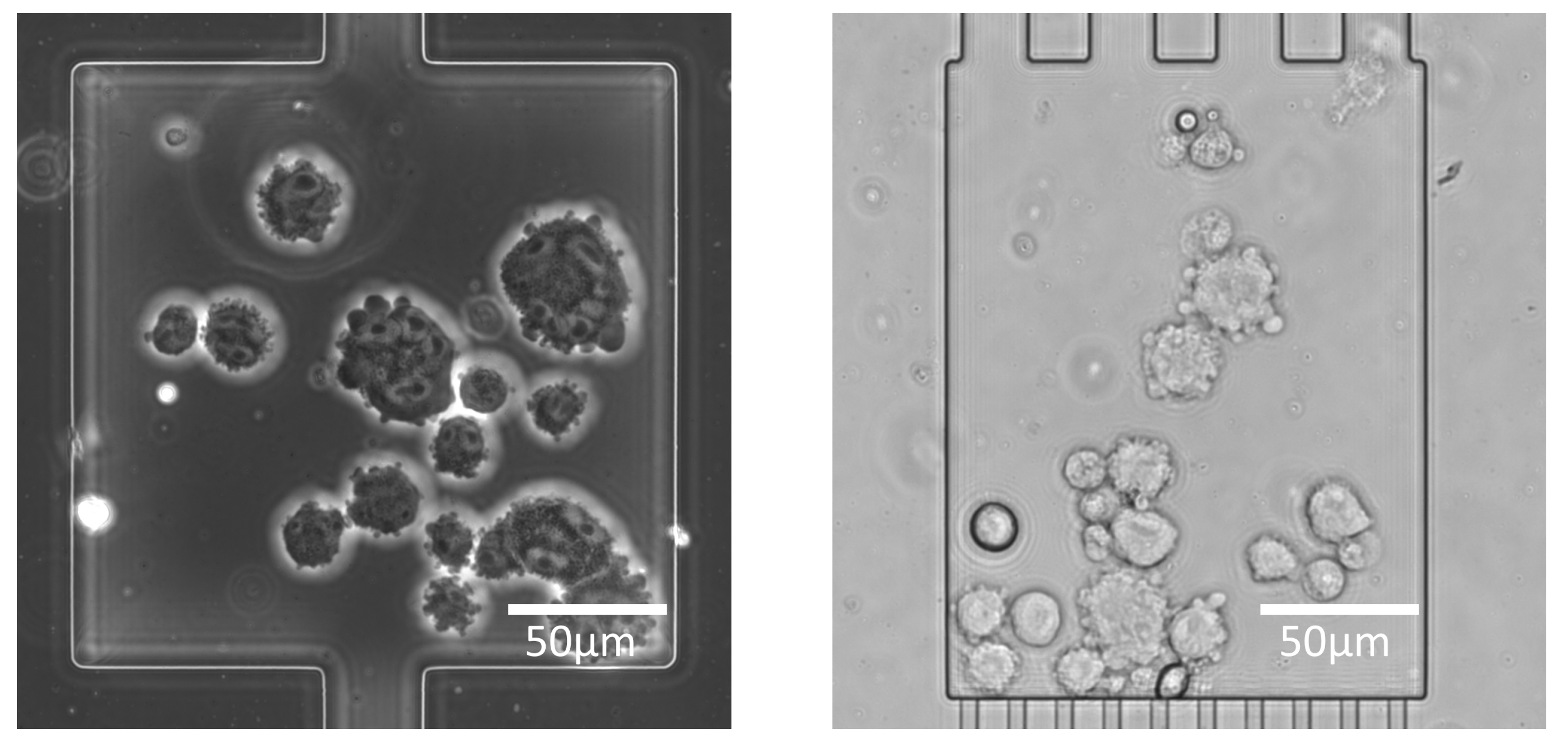
• Ongoing cell divisions (Figure 1 right), making it unclear in some cases what the actual correct target variable would be, but giving a meaning to comma values as they can represent an ongoing division.
• Varying contrast and light conditions.
• Dying, appearance, and vanishing of cells.
• Overpopulation of the cell chamber or the end of an experiment due to escape of the cells.
• Overlapping and close adherence of cells.
• Continuous changes in the cell membrane and inner organelles, changing the orientation of cells, with variations in shape and perceived size.

In this article, we propose a novel training scheme for a Siamese deep learning model that can optimally combine information provided by automatically generated synthetic data and real images such that no manual labeling of natural data is required. The contribution and novelty of this work are as follows:

• We achieve high prediction preciseness on the target variable where the state of the art fails to do so.
• We build an effective translation learning pipeline and show, on multiple microscopy data sets, that this pipeline is stable and reliable throughout this domain.
• We gain additional insight into the inner state of the neural network by performing translations twice (cycling), leading to critical parts of the architecture to optimize the network for the domain without overfitting to the specific data, thus contributing to the understanding of deep neural network representations, especially for Siamese networks [6].

In the following sections, we first give an overview of the current state of the art in this research field and take a brief look at previous works in this field of application. In Section 3, we address the underlying machine learning challenge and present our deep Siamese network architecture in detail. Then, the details of the proposed learning procedure are explained and it is analyzed how the unique architecture used affects the learning procedure. Thereafter, Section 4 contains the evaluation for real data sets and ablation studies, as well as the comparison to state of the art alternatives and baselines. Lastly, in Section 5, a discussion followed by a conclusion (see Section 6) completes the contribution.

2. Related Work

In the last few years, convolutional deep neural networks have become the state of the art for image processing that does not require human labor and for the majority of other computer vision tasks  [7]. Especially for the task of counting in images, solutions have been worked on for over a decade now (see [8]). Applications in the biomedical domain have become common [9] and cell tracking approaches in images have been an ongoing field of study in recent years [10]. However, the optimization of such methods is often time-consuming and remains prone to errors.

Ulman et al. [11] propose a benchmark suite to compare different imaging technologies and extrapolate the strengths and limitations of different approaches to cell tracking, none of which have been determined as a final solution on this task, even the ones including interactions among bioimage analysis experts [12] or the distributed work of manual labeling [13]. Schmitz et al. [14] show the demand for fleshed out solutions by evaluating the currently used state of the art tools as insufficient for heterogeneity studies of the CHO-K1 mammalian cells that are present in the given data.

In addition, Brent et al. [15] used transfer learning to predict microscope images between different imaging technologies, but without sufficiently accounting for the wide variety of cell images and features. The approach by Falk et al. [16] provides one of the few toolboxes for cell tracking, albeit for adherent rather than suspension cells. It allows for transfer learning based on given models and novel data, whereby data set enrichment technologies limit the number of required samples.

In contrast to adherent cell lines, where already reported single cell cultivation studies [17,18] promise success, we address the more complex scenario of suspension cells with all their visual characteristics listed above, rendering analysis tools of adherent cells deficient. Earlier works have overcome some of the challenges, such as sufficient counting accuracy, by interactive design [19], or detecting overlapping instances in such imagery [20], but they are not yet sufficient for the unsupervised task at hand. Different contrast and light conditions have been addressed by Chen et al. [21]. The adherence of cells and overlaps have been addressed by Xie et al. [22], but additional visual features complicate the process and reduce the applicability of previous solutions.

Siamese networks have been used for a variety of tasks as they can help to facilitate few-shot learning or clustering of the data space by generalizing from unlabeled data. This is done in [23] for genome sequencing and in [24] for text data. These presented architectures are, however, specific to their domains and not applicable to image processing.

There are also Siamese networks that do work in the image processing domain, such as [25], but they focus on change detection as a binary segmentation, suitable for tracking single cells, but not for the regression task at hand. Ref. [26] uses Siamese networks and data augmentation, similar to our approach, but the training is supervised and addresses a four-class classification task. In [27], similar data augmentation and Siamese networks were used and the 20-class classification is closest to the regression task that we address, but the networks used are non-generative CNNs and the data are not used cyclically, rendering it not applicable for our work.

Furthermore, there are no deep learning models that easily and efficiently solve the task, as shown in [3] by comparing the recent state of the art EfficientNet [28] and classical image processing such as Watershed methods [29], and transfer models such as BigTransfer [30] are not reliably able to generate good cell counts by transferring a pretrained model to this domain, as can be seen in our earlier work [4].

Deepak Babu et al. [31] achieved acceptable accuracy for the regression task of crowd counting, a similar task; however, the training was semi-supervised. More generalized few-shot and even zero-shot learning has been done by Schönfeld et al. [32] by using aligned VAEs, achieving high precision, but only on the few-shot tasks, not the zero-shot ones. In our approach, we will fully focus on the idea of the integration of synthetic data, which can itself harvest its semantically meaningful generation, to avoid any additional manual labeling of natural data for training, therefore rendering even these related results insufficient.

Synthetic data have already been used in [33,34], but for natural scene and text recognition, or computer vision tasks more generally, mostly natural domains where powerful deep generative models can build on massive amounts of publicly available data. In contrast, we are interested in synthetic data that are prone to a reality gap due to the limited availability of natural data. In semi-supervised learning, models are often enriched by easily available unlabeled data that describe the underlying input distribution [35]. A view into when unlabeled data can improve the learning rate has been taken by Göpfert et al. [36], suggesting the usage of additional unlabeled data, be it synthetic or natural, as beneficial, confirmed for this case in Section 4. The impact of variability in auxiliary training data on convolutional networks specifically was tested in [37], but for 3D head reconstruction, not intrinsically usable in this domain.

The weight sharing used in our particular learning scheme was used previously to decrease network sizes and improve test and verification performance [38]. In Section 3.3, we show details on the specialized usage of this technique for our architecture.

Lastly, Uniform Manifold Approximation and Projection (UMAP) [39] is used to project the inner state of the network into a two-dimensional representation, allowing us to obtain a glance at the internal state of the latent representation and insight into how the data are processed. In Section 6, such a UMAP is discussed for interpretation.

3. Methodology

3.1. Natural Data

Image data applied in this study were obtained by MSCC of mammalian suspension cells, as introduced before in the literature [40]. The CHO-K1 cells were cultivated in polydimethylsiloxane (PDMS) glass chips. Perfusion of the device constantly provided the cultures with nutrients. An automated inverted microscope performed the live cell imaging, taking images of the relevant positions on-chip every 20 min. The data used in this work are split into two major parts according to the two microscopy technologies, namely bright-field microscopy and phase-contrast microscopy, abbreviated as BF and PC, which were used for the analysis of the architecture. Figure 2 shows example data from both microscopy technologies after the application of the preprocessing described below.

Around 10,000 images were taken over the course of the experiments per microscopy technology; then, images of empty and fully filled cell chambers were removed, since, for these, the experiment had not started yet or the outcome of the experiment was already determined, respectively. In total, 2983 BF images and 3944 PC images remained relevant for the machine learning task. Around 20% of the data were labeled by hand exclusively for testing and will from here on be called Nat-L-Te (natural, labeled test data); the other 80 percent remain unlabeled and are used for training and called Nat-U-Tr (natural, unlabeled training data). The test data were split in half to obtain a verification data set and to prevent accidental specialized training on the test data over the course of the hyperparameter optimization. During the test data selection process, we ensured that full experimental runs as well as randomly picked images from the various experiment series were part of the test and verification data.

Table 1. Overview of all data sets used. Nat-U-Tr  contains natural, unlabeled training data; Nat-L-Te  natural, labeled test data; Syn-L-Tr  synthetic, labeled training data, and Syn-L-Te  contains synthetic, labeled test data. For reasons described in Section 3.2, synthetic data have been generated in a 1:1 ratio to natural data. Nat-PC  refers to all natural phase-contrast images (i.e., Nat-L-Te  and Nat-U-Tr) and Nat-BF  refers to all natural bright-field images, respectively. Syn-PC  and Syn-BF  denote the groups of training and test data for phase-contrast and bright-field data accordingly, and, lastly, Nat  and Syn  denote the full set of natural and synthetic data.

Data Set Name	No. of Phase-Contrast Images	No. of Bright-Field Images
Nat	Nat-PC	Nat-BF
Nat-U-Tr	3.152	2.469
Nat-L-Te	792	514
Syn	Syn-PC	Syn-BF
Syn-L-Tr	3.152	2.469
Syn-L-Te	792	514

gives an overview over the different types of data sets used in our work.

We crop and rotate all images to center the cultivation chamber. Further data augmentation beyond this preprocessing is described in Section 3.2. We place our focus on the larger data set called Nat-PC from here on. It contains more experimental samples and the biological processes covered are more diverse. In addition, phase-contrast microscopy is more popular, and we will nonetheless show that our method also works reliably on the smaller Nat-BF data set, although the variations in cell positions, numbers, and sizes are lower in this data set and therefore the quality of these images is lower in terms of machine learning, similar to what might be the case for entirely different types of cells, such as plant cells.

To make the best use of the poor amount of experimental data, the following enrichment techniques are applied to the data. Flips along both image axes are followed by a random crop up to the edges of the cell chamber, not cropping away cells, except for the entrance tunnel, where precise cell detection is not required. The crop does complicate cell detection, as cells may be in positions where only the chamber rim and the outside of the chamber would be without the crop, but it proved necessary to allow cells to appear anywhere on the images to ensure uniform detection success that is barely affected by the position of the cells within an image. Then, a random rotation of 90${}^{\circ }$ is performed and a randomly generated noise map is multiplied by a small weighting factor and applied to the image to simulate more fluctuation in the cells’ visuals, since occasionally there are dead cells in the experimental data that do not change in appearance for multiple images. All augmentations are reapplied to the original data for every epoch of training with seed consistency to ensure reproducibility.

3.2. Synthetic Data

We propose a novel learning scheme in Section 3.3.2 that deals with synthetic data with known ground truth (i.e., the cell count) and a Siamese architecture that can abstract from the fact that the auxiliary data are synthetic. In addition to the common data set enrichment, generating proxy data allows us to create a wide variety of synthetic samples, which are inspired by the natural data, but not limited by their amount or variety.

By enriching the training procedure with synthetic data, we extinguish the need for natural labeled data. Synthetic data are easily obtained in this setting because the architecture does not require that the images are rendered realistically in all respects, such as morphological details. The 128 × 128 working resolution of the architecture makes the synthetic data generation undemanding, while maintaining sufficient intricacy of visual features such as overlapping (see Figure 3 left). For the specialized training procedure described below, we do not need to synthetically create images that are indistinguishable from natural ones, unlike current data augmentation schemes, such as proposed in the work [41]. This would require a considerate amount of engineering [37], i.e., human expert labor, exactly what we aim to mitigate. We rely merely on modeling simple ellipsoidal shapes to embody cells, ignoring details of the texture and the intricate morphology of real suspension cells. We imposed this limitation on ourselves to suggest that the learning procedure presented below should also work with other types of image data and is neither tailor-made for exactly these microscopy technologies nor requires extensive manual work to generate the most realistic synthetic data possible. In Section 3.3, we show that this approach is adequate for training our architecture described.

We ensured that the distribution of cell counts in the auxiliary data was sufficiently close, but not necessarily identical to that of the natural data sets. This allows for an unlimited amount of labeled training data, with only the processing time being the limiting factor for the potential to use enormous amounts of proxy data, not the availability of such. One problem remains, however, which is how to actually improve the regression performance on natural data. Using a large ratio of synthetic data compared to natural data would entail a separation of the two types of data in the inner representation of the network, resulting in high accuracy on the synthetic data, but low accuracy on the natural data (see Section 4). To prevent this separation, two major functionalities are proposed and have been implemented, described in more detail in the following paragraph.

The auxiliary data generator is highly adjustable and produces imagery with a given distribution of cells. As background images, we calculate the mean of the first 20% of data from the experimental series, expecting cell counts to be low and cells to be scattered, so that the background has no visible natural cells in it. The generator takes control of the overlaps, brightness, and blurriness of the cells’ inner organelles as well as their membranes, the contrast with the background, a range of possible cell sizes, counts, and crop values, as well as the ellipsoidal deformation range as parameters. All these can be chosen by hand within the code package, or the default values can be used. Combined, these operations can be used to imitate most of the intricate features of the real data, such as ongoing divisions of cells, by requesting a small overlap along with noisy cell boundaries. Smudges, as in Figure 2, are not included because they are a confounding factor and are assumed to only hinder the training process. The cells have been given a roughly circular shape to approximately match the shape of the natural cells. To generate cells, positions are sampled randomly from the valid space, taking the parameter of possible overlaps into account, and are then randomly stretched, deformed, made noisy, and so on according to the chosen parameters; then, brightness fluctuation and Gaussian filters of varying strengths are added to increase the variety of cells in the data. This geometric form can easily be adjusted if natural cells in other data sets have different shape characteristics or when other camera setups produce different ambiences.

This data are generated fully automatically based on simple algorithmic principles and, as a baseline, a ratio between synthetic and natural data of 1:1 is used, since larger amounts increase the training time almost linearly, while the performance improves only with diminishing returns in our experiments. More details on this are given in Section 4. The imagery is produced algorithmically with seed consistency and can therefore be reproduced similarly to the data enrichment on the natural data and can be generated in an arbitrary amount.

3.3. Architecture and Learning Scheme

3.3.1. Architecture

Our aim is to provide reliable cell counting for the microscopic imaging of suspension cells, and since the experimental data are limited in their amount and without annotations, we assemble a novel learning scheme for the Twin-VAE architecture previously introduced by us to overcome these limitations.

The architecture circumvents the problem of differences in the appearance of auxiliary and real data by separating the data input for training according to their origin, but requires that the model creates a tightly coupled joint inner representation to avoid high training losses. This is realized by modifying a Variational Autoencoder (VAE), duplicating the outer layers of the encoder and decoder, accounting for the two data sets. Therefore, the weights of the inner layers of both encoder and decoder are shared, as well as the semantic bottleneck in between (see Figure 4). We decided to choose this architecture for the reasons mentioned in Section 2.

The specialized encoders consist of four two-dimensional convolutional layers with kernel sizes of 5 and strides of 2. They are initialized with an orthogonal basis [42]. In between layers, leaky rectified linear units (LReLUs) with a leakiness of $0.2$ and a dropout of $0.1$ have been added. The channels used for the convolutions in the encoders in order are 32, 64, 128, and 256. The weight-shared encoder contains a single two-dimensional convolutional layer with the same remaining attributes but 512 channels. It is followed by the bottleneck, consisting of three layers of fully connected neurons. The layer sizes are 512, 256, and 512, each with the same dropout as before. The weight-shared decoder therefore also has 512 channels and uses a two-dimensional transposed convolutional operator layer with identical strides and kernel sizes as above, followed by a batch normalization over a four-dimensional input and another LReLU with the same leakiness. The decoders designed for specific data each consist of a total of five layers with kernel sizes 5, 5, 5, 2, 6, and strides of 2, 2, 2, 1, 2, following the convention of a smaller second to last kernel followed by a large last kernel. Then, we include the same LReLUs and a sigmoidal activation function at the end.

The representation in the latent space is not only fed to to the weight-shared decoder, but also to a three-layer fully connected network of neurons as a regressor. The sizes of the layers are 256 and 128 and lastly 1. Linear layers and a dropout of $0.2$ are used for the regressor. The rectified Adam (RAdam) [43] optimizer worked best for the training procedure.

One of the VAEs works on proxy data, and we will refer to it as VAE-syn, while the other one processes natural data (VAE-nat). The differing visual features of proxy and real data are accounted for in the separated layers, while the weight-shared encoder and decoder rely on and enforce a similar representation of the determinant image characteristics. In addition to auto-encoding, the architecture works on data with known labels in a supervised manner by the addition of a three-layer fully connected neural network regression model for the actual cell counting, based on the shared representation of the VAEs.

3.3.2. Learning Scheme

For images x of either natural or synthetic type $t\in \{\mathfrak{n},\mathfrak{s}\}$, the VAEs are able to generate reconstruction losses $Rec(x,y)$ from reconstructed images y of their decoder. $C_{Rec}^t$ are hand-crafted weighting factors to balance the different reconstruction costs. Choosing these weights to be large results in better reconstruction but worse regression. However, proper reconstruction quality is required to fabricate well-trained encoders, thus demanding the factors to not be too low. The loss for the reconstructions is defined as

$$\begin{array}{c}\hfill RE{C}_{loss}(x,t)=C_{Rec}^n·Rec(x_n,y_n)+C_{Rec}^s·Rec(x_s,y_s)\end{array}$$

(1)

For synthetic data with cell counts l from 1 to 30, we can also generate a regression loss $Reg(x_{\mathfrak{s}},l)$. However, $Reg(x_{\mathfrak{n}},l)$ cannot be calculated usually, since l is not known for these. In Section 4, our ablation studies show that this is insufficient for effective regression on natural data. The internal representations of the two types of images are naturally being separated in the bottleneck, precisely what VAEs are usually known and used for, resulting in high precision for synthetic data, but nearly arbitrary cell counts for natural data.

The specialized architecture allows an additional learning scheme to generate a loss for pseudo-natural data. This is done by encoding synthetic data in their specialized encoder, but decoding them with the decoder designed for natural data. This translation works both ways and will result in images $x_{\mathfrak{s}\to \mathfrak{n}}$ and $x_{\mathfrak{n}\to \mathfrak{s}}$.

This new type of data can now be used in the natural pipeline, creating new reconstruction losses $Rec(x_{\mathfrak{s}\to \mathfrak{n}},y_{\mathfrak{s}\to \mathfrak{n}})$, which can be used to train the according encoder and decoder, especially enriching the data available for the natural pipeline immensely.

These images will be called translated or cycled images from here on and they expand the usable image types to $t\in \{\mathfrak{n},\mathfrak{s},\mathfrak{s}\to \mathfrak{n},\mathfrak{n}\to \mathfrak{s}\}$. Examples of translated images and a pipeline of their generation can be seen in Figure 4. Cycled images also generate reconstruction losses, which are defined as

$$\begin{array}{c}\hfill REC-T_{loss}(x,t)=C_{Rec}^{n\to s}·Rec(x_{n\to s},y_{n\to s})+C_{Rec}^{s\to n}·Rec(x_{s\to n},y_{s\to n})\end{array}$$

(2)

These images do not exactly resemble natural images and are distinguishable from them by the human eye, but they are actually close enough in their relevant characteristics to natural images that when designing the learning scheme in the way described below, they are not distinguished as fake natural images by the architecture, a beneficial circumstance that allows the simulation of labeled natural data and shared representations, which becomes more clear when taking a look at the UMAP of the internal representation later in Section 4.3.

This process also leads us to translated natural images, for which the label is known, and therefore allows for the generation of the regression loss $Reg(x_{\mathfrak{s}\to \mathfrak{n}},l)\ne 0$. This way, we can train the full regression pipeline for natural data, without any labeled natural data at all. Henceforth, we refer to this process as translation learning.

Furthermore, we can translate the same images again, leading to two new types of images yet again $t\in \{x_{\mathfrak{s}\to \mathfrak{n}\to \mathfrak{s}},x_{\mathfrak{n}\to \mathfrak{s}\to \mathfrak{n}}\}$, which should appear near-identical to the original reconstruction y. We first designed this difference to be a loss as well, but we later omitted this training step for hyperparameter optimization, as it did not improving the accuracy on cell counts significantly while adding another step of the more demanding image backpropagation to the pipeline. However, we still create these bilateral translations for specialized top-performing models (see

Table 2. Evaluation of all baselines and SC-VAE on the data sets Nat-PC, Nat-BF, Syn-PC  and Syn-BF. For each method and data set, we report the mean absolute (MAE), the mean relative error (MRE), and the accuracy. Ultimately, only performance on natural data (Nat) is important, but we also report the performance on synthetic data (Syn) to provide further context. We use an upward arrow ↑ to indicate that higher is better; a downward arrow ↓ means lower is better. The best results achieved per category are marked in bold, (ss) denotes a semi-supervised method, (u) an unsupervised method.

Method	MAE (Syn) ↓	MRE (Syn) ↓	Acc. (Syn) ↑	MAE (Nat) ↓	MRE (Nat) ↓	Acc. (Nat) ↑
PC  (phase-contrast microscopy)
EfficientNet (ss)	4.987	79.4%	5.0%	1.67	25.12%	23.4%
BiT (ss)	N/A	N/A	N/A	2.32	29.7%	25.4%
Twin-VAE (ss)	0.09	0.68%	68.2%	0.60	5.92%	57.8%
Transfer Twin-VAE (ss)	0.15	0.43%	85.0%	0.66	6.46%	53.7%
Dual Transfer Twin-VAE (ss)	0.12	0.43%	85.0%	0.58	5.56%	58.7%
Watershed (u)	0.94	18.0%	24.0%	1.66	29.0%	23.1%
C-VAE (u)	0.24	2.65%	54.2%	1.03	19.1%	28.9%
S-VAE (u)	0.09	0.53%	76.3%	2.64	41.2%	11.6%
SC-VAE (u)	0.11	0.83%	66.1%	0.49	5.16%	61.7%
SC-VAE-B (u)	0.10	0.81%	67.9%	0.48	5.12%	61.8%
BF  (bright-field microscopy)
EfficientNet (ss)	6.502	67.1%	4.5%	1.13	17.2%	33.9%
BiT (ss)	N/A	N/A	N/A	1.79	22.45%	38.7%
Twin-VAE (ss)	0.48	4.27%	60.1%	0.68	7.6%	53.2%
Transfer Twin-VAE (ss)	0.40	3.87%	66.6%	0.52	5.47%	60.7%
Dual Transfer Twin-VAE (ss)	0.35	3.73%	66.8%	0.51	5.43%	60.8%
Watershed (u)	1.92	39.0%	2.0%	2.39	32.0%	32.0%
C-VAE (u)	0.67	5.72%	50.8%	1.96	21.8%	26.3%
S-VAE (u)	0.33	3.66 %	67.3%	2.09	34.2%	18.6%
SC-VAE (u)	0.41	3.88%	62.5%	0.60	7.1%	56.6%
SC-VAE-B (u)	0.39	3.77%	62.6%	0.56	6.51%	58.7%

) and for reasons mentioned below. Since the cycling of data through the different types is what allows the architecture to perform a regression task on unlabeled natural data, we call it Siamese-Cycle-VAE or SC-VAE for short, and variants with enabled bilateral learning cycles will be called SC-VAE-B from here on.

As mentioned above, we also generate pseudo-synthetic data $x_{\mathfrak{n}\to \mathfrak{s}}$ from natural data (blue arrow in Figure 4). Since, for these pseudo-data, annotations are unknown, they cannot be used to train the regression process, but they can be used for two different purposes.

The first is balancing out the encoders and decoders, since, with the learning scheme described above, the synthetic pipeline will go through more training steps than the natural one, although this is the one that should be especially well-trained, as the minimization of regression losses on natural data is the actual goal of this learning scheme. In this way, the natural training pipeline can also be trained on many more cell arrangements than the few that natural images provide, since even with a multitude of data augmentation techniques, the generalization of encoding and decoding can be improved by this step (see Section 4).

Secondly, the decodings of translated synthetic images $y_{\mathfrak{n}\to \mathfrak{s}}$ can be used as stability checks of the latent space for the different types of data. Badly decoded pseudo-synthetic images imply a larger than wanted differentiation of natural and synthetic images in the bottleneck. More on this is given in Section 4.1.

Considering the loss functions, let $r\left(x\right)$ be the estimated cell count and l remain the label. The mean-squared error (MSE) $\left|\right|r\left(x\right)-{l\left|\right|}^2$ and the binary cross-entropy (BCE) $-l·log\left(r\right(x\left)\right)+(1-l)·log(1-r(x\left)\right)$ yielded similar results as in our previous works, and both resulted in more precise cell counts than common alternatives; therefore, extensive testing has been done with both, but ultimately the MSE was chosen as the default, since it is easier to find appropriate coefficients for the different types of losses due to the diminishing nature of MSE. The weight factors determine the importance of the counting accuracy and change over the course of the training procedure, since deriving accurate cell counts on natural data from synthetic and translated data requires preceding training of the encoders and decoders. The associated $RE{G}_{loss}(x,y)$ term is defined as

$$\begin{array}{c}\hfill RE{G}_{loss}(x,l,t)=C_{Reg}^{s,l}·Reg(x_s,l)+C_{Reg}^{s\to n,l}·Reg(x_{s\to n},l)\end{array}$$

(3)

When using BCE, the decoder loss factors decays over time with a decaying rate of $3\times {\mathrm{10}}^{-5}$ per epoch. This is necessary because the BCE does not decrease significantly during training, but needs to diminish over time to increase the importance of low regression losses $Reg(x,l)$.

Since it is beneficial for the prevention of overfitting to generate latent vectors that are sufficiently close to a normal distribution, we aim for homogeneous representations of synthetic and natural data in the embedding space of the architecture by applying a regularization cost ${\mathcal{D}}_{\mathrm{KL}}$, which is applied in the form of the Kullback–Leibler divergence (KLD) of the standard VAE [44]. This loss will also ensure that the inner representations of natural, synthetic, and both types of cycled data stay similar, allowing us to use the special training procedure described above. This cost is applied for natural, synthetic, and both types of translated data and is defined as follows:

$$\begin{array}{c}\hfill KL{D}_{loss}(x,t)=C_{{\mathcal{D}}_{\mathrm{KL}}}^{n,n\to s}·{\mathcal{D}}_{\mathrm{KL}}\left(x_{n,n\to s}\right)+C_{{\mathcal{D}}_{\mathrm{KL}}}^{s,s\to n}·{\mathcal{D}}_{\mathrm{KL}}\left(x_{s,s\to n}\right)\end{array}$$

(4)

All coefficient factors have to be chosen mindfully, balancing the main target of punishing incorrect cell counts on natural data and relaxing the importance of details in visual reconstruction, but not undervaluing the KLD at the same time. Doing so can make the training procedure unstable, while applying very large regularization costs hinders the learning process and slows it down. To minimize the number of hyperparameters that have to be optimized by hand, the weighting factors for the ${\mathcal{D}}_{\mathrm{KL}}$ losses have been grouped and a Bayesian optimization [45] in the form of a Gaussian process regressor [46] was used to quickly find baseline values for the most important hyperparameters, such as the learning rate and the loss weight factors.

We combine these losses to form our overall ${\mathrm{SCVAE}}_{\mathrm{loss}}(x,l,t)$, use the coefficients of the different terms to balance the impacts between natural, synthetic, and both types of translated images, and handle input images with missing cell counts by fixing $C_{Reg}^{\mathfrak{n},l}=C_{Reg}^{\mathfrak{n}\to \mathfrak{s},l}=0$:

$$\begin{array}{c}\hfill {\mathrm{SCVAE}}_{\mathrm{loss}}(x,l,t)=RE{C}_{loss}(x,t)+REC-T_{loss}(x,t)+RE{G}_{loss}(x,l,t)+KL{D}_{loss}(x,t)\end{array}$$

(5)

3.3.3. Baselines

For the evaluation in the upcoming section, several baselines have been gathered, to enable a meaningful comparison with the state of the art. The first baseline is a widely practiced classical computer vision pipeline. First, the input images are cropped to only contain the cell chamber, and are then blurred with an averaging kernel-based filter; then, a thresholding filter is applied, followed by a watershed segmentation [29]. The regions of the segmented image are counted and used as a cell estimation. In order to find suitable parameters for this learning scheme, an exhaustive grid search was performed for each data set BF and PC. The code repository contains the best hyperparameters found. We refer to this pipeline as Watershed in the following.

As a second baseline, we fine-tuned a pre-trained state of the art deep convolution neural network, specifically a variant of EfficientNet [28]. We replace the last layer of the pre-trained network with a fully connected layer that outputs a single value, and train it to predict the cell count for a given input image. We apply the same hyperparameter optimization as for our own method, and generate the same data augmentation. Since EfficientNet is a variable architecture that comes in different sizes, referred to as EfficientNet-B0, EfficientNet-B1, and so on, we evaluated EfficientNet-B0 through EfficientNet-B3 and found that the smallest variant EfficientNet-B0 performed best, while larger variants performed progressively worse. We considered to instead use EfficientNetV2 [47], but our preliminary results showed that the same performance degradation applies to its larger variants as well, and since EfficientNet-B0 outperformed the smallest EfficientNetV2-S variant, we retained it and refer to this fine-tuned convolutional neural network as EfficientNet hereafter.

As a third baseline, we compare a state of the art transfer learning model from Kolsenikov et al. called BiT, which produces highly accurate classification results on Cifar-100 and similar data sets in a few-shot learning case of 1 to 10 examples per class. BiT consists of the classical ResNet [48] architecture, but with very long pre-training times on large image sets and a custom hyperrule that determines the training time and learning rate during transfer depending on the size of the new data set. Changes to the hyperrule were tested, but did not cause any significant improvement in accuracy; therefore, the values provided by the authors were used. BiT is given all the natural and synthetic training data per epoch, so it can come up with meaningful cell counts on natural data by abstracting from the labeled synthetic data. We valued the possible cell counts from 1 to 30 as classes, to account for the difference in training methodology.

In addition, we compare our own previous work Twin-VAE  (see [3]) and its alterations Transfer Twin-VAE  and Dual Transfer Twin-VAE (see [4]). These are based on the same architecture, but perform semi-supervised learning techniques for which the same data are used, albeit with partial annotations on the natural training data of 5–10%. Although this circumstance should allow for higher accuracy on the counting task, the optimized pipeline and cyclic data reuse of the new Siamese-Cycle-VAE is able to keep up with and in some cases even outperform its predecessors, despite not being given any manual labels at all. More on this is given below.

Lastly, ablation studies are done to ensure and show that the specific architectural details and principles of the learning scheme are helpful and optimize the training procedure and therefore the accuracy on the regression task. One study will be called C-VAE from here on. In this alteration of the network, there are no specialized Siamese encoders and decoders, but the cyclic structure is kept. C-VAE should still be able to make meaningful cell predictions, albeit that the abstraction between natural and synthetic data has to happen in the inner layers of the VAE. The cyclic structure and the difference between original and reconstructed images can still help the architecture to enrich the data in a more extensive way than classical data augmentation alone can. The second study is called S-VAE. Here, the Siamese architecture is kept, but we omit the cycling and do not use the reconstructed image data as new input, but merely as reconstruction loss, as in the standard VAE. As there are no labels on the natural data and there is no translated pseudo-natural imagery with labels either, the regressor lacks a loss to meaningfully train for this type of data directly, but could possibly abstract from the differentiation between natural and synthetic data in the latent space and still achieve adequate accuracy on cell counting.

4. Results

As for the hyperparameter choices, the best results were achieved with decoder loss factors $C_{Rec}^{\mathfrak{n}}=1\times {10}^2$ and $C_{Rec}^{\mathfrak{s}}=2\times {10}^2$, with the higher loss on synthetic data accounting for the higher image variety of these images, while $C_{Rec}^{\mathfrak{n}\to \mathfrak{s}}=C_{Rec}^{\mathfrak{s}\to \mathfrak{n}}=5\times {10}^1$ resulted in the lowest reconstruction losses. While not mandatory to minimize, a degradation in the deconstruction loss of translated images is almost always coupled with lower regression losses. The regressor loss factors for synthetic data $C_{Reg}^{\mathfrak{s}}$ and pseudo-natural data $C_{Reg}^{\mathfrak{s}\to \mathfrak{n}}$ are both set to 5 and should inversely account for the ratio between the according types of data. The KLD factor $C_{{\mathcal{D}}_{\mathrm{KL}}}=1$ yields the best results for the larger data set Nat-PC, while slightly larger factors work better for Nat-BF, constraining the inner representations of synthetic, natural, and translated images to be coupled tightly. Faster convergence was observed for smaller KLD factors, but the learning scheme tended to separate more between data types, resulting in better reconstructions but poorer regressions. Figure 5 shows the combined losses and indicates convergence.

In addition, a soft weight decay of $2\times {10}^{-5}$ per epoch, a constant learning rate of $0.75\times {10}^{-5}$, and delaying the start of the regressor by 25 epochs are used to achieve the following results. Batch sizes of 128 for both types of microscopy imagery work best and the training runs for up to 20,000 epochs, as there are no significant improvements after this. Ablation studies with more synthetic data relative to natural data have been done as well. In general, the architecture appears to converge faster when measured by epochs, but when taking the increase in training batches per epoch into account and therefore measuring by the number of computations, the training speed is marginally lower in all cases, so we retain the 1:1 ratio.

4.1. Comparison

We present the results of our method and the comparative baselines in Table 2. The mean relative error (MRE) is a normalized error, taking the ground truth into account, i.e., in high cell count images, small absolute deviations do not increase the error as much as they do for low cell count images. When interpreting experimental results as a biological expert, in most cases, this is the more meaningful indication over the mean absolute error (MAE), which serves as the typical indicator in terms of a regression task. The bilateral alteration SC-VAE-B that uses fully cycled images (back and forth) results in marginal but reliable improvements, assimilating representations in the latent space, and should be considered our top candidate.

Our SC-VAE consistently outperforms the other state of the art methods Watershed, BiT, and EfficientNet by a wide margin. SC-VAE and its alteration SC-VAE-B correctly estimate around 62% of the cell counts for the Nat-PC data set, and their predictions differ on average by only 0.5 cells from the true cell counts of the images, and they achieve approximately 5.1% MRE. For the smaller Nat-BF data set, SC-VAE-B accomplishes $0.56$ MAE, $6.5$% MRE, and 58.7% accuracy. While Dual Transfer Twin-VAE achieves slightly better results for these data, they are attained by semi-supervised training, commonly not even compared to unsupervised methods. As such, Siamese-Cycle-VAE holds up against semi-supervised training methods and even exceeds them the case of the larger Nat-PC data set, making it suitable for reliable cell counting with various microscopy techniques.

Moreover, we see that Siamese-Cycle-VAE performs well across the entire range of cell counts in Nat-PC and Nat-BF. By contrast, Watershed and EfficientNet struggle with images that contain few cells, which is the most important range of cell counts for biological tasks, such as estimating the growth rate.

The ablation C-VAE that feeds all data through the same encoder and decoder results in accuracy on synthetic data that is inferior to the other methods, even more so for the important accuracy on natural data. By using the reconstructed images as new input, the learning scheme resembles the optimized scheme of SC-VAE in such a way that visual intricacy on natural data is simplified, but not on the same level as SC-VAE..

S-VAE, on the other hand, worked best on synthetic data, especially so for Nat-BF, but for both types of microscopy data, the MRE and accuracy on the natural data are far from the results from SC-VAE. No translated natural data are generated by S-VAE, which is missing the regression loss for natural data completely. Cell counts on natural data are not random since there is still the shared encoder to unify the two types of data, but since accuracies differ vastly between natural and synthetic data, the S-VAEs encoder fails to do so because of a missing incentive.

4.2. Image Reconstruction and Representation

An analysis of the reconstruction abilities of Siamese-Cycle-VAE is useful to ensure that the shared representation is meaningful, even though our main aim is automatic cell counting, not perfect image reconstruction.

During the training of Siamese-Cycle-VAE, the image inputs are processed by their respective encoder, followed by the general, weight-shared encoder, represented in the bottleneck of the architecture; they are then processed by the shared decoder and finally reconstructed by their specialized decoder accordingly (see Figure 4). The same is true for auxiliary data and both types of translated pseudo-imagery. To ensure that the actual regressive task works as intended for natural images, it must be able to benefit from synthetic data representations in the latent space, so the learned representation must be shared by the four types of data.

This can be verified by encoding natural images with their appropriate encoder, but performing the decoding with the decoder that is designed and trained for auxiliary images, the counterpart to the opposite conversion, which is done in every epoch of training. Minimal changes in the stages of the images that are converted back and forth indicate the close coupling of the representations. The closer the different data types are transformed into the latent space, the greater the potential gain for regression on natural data. Moreover, the conversion makes this fact interpretable on a visual level.

We show examples of perfect translations in Figure 6. For these samples, a natural image is encoded and then decoded as a synthetic image. The number of cells remains unchanged, and the position and size of the cells are also maintained. However, the overall appearance is simplified: Siamese-Cycle-VAE learned to remove noise and to break down the reconstruction to the essentials. Even the very large smudge on the left natural image has not been reconstructed; although it will cause an increased loss in the reconstruction, the weighting of the loss factors makes it more acceptable to forfeit image reconstruction precision in favor of the regression. On the right side, it can be seen that the output does indeed appear more similar to natural data than the synthetic input does, while fine details such as the noisy borders are not recreated.

The ongoing cell division shown in Figure 7 is a prime example to understand how Siamese-Cycle-VAE works. The membrane of the bottom right cell is not fully enclosed and there is no overlap, since a fine bright border of the underlying cell would be seen through the top cell. However, two cell cores can clearly be seen and a human expert would presumably count this situation as two cells, which is exactly what Siamese-Cycle-VAE does. The prediction of $9.65$ instead of 10 can be understood as uncertainty and a slightly earlier stage of the division would have arguably led to a slightly smaller prediction, which, when rounded, would be the correct cell count again. The effect of simplified visuals also happens in these non-translated reconstructions; the smudges on the Nat-BF sample are clearly fainter and, in the left image, even the high-contrast dead cell residue on the left is not recreated. This clearly indicates that even when Siamese-Cycle-VAE does not predict the cell count perfectly in an image, the comparison between the original and reconstructed image is useful to understand where an error occurs.

4.3. Shared Representation

Siamese-Cycle-VAE’s ability to translate back and forth between natural and synthetic images illustrates the semantically shared representation of all four types of data learned by the autoencoder. Below, we visualize this shared representation. Because each image is encoded as a 256-dimensional vector, we need to reduce the dimensionality to do so. Uniform Manifold Approximation and Projection (UMAP) [39] has established itself as the state of the art for nonlinear dimensionality reduction. It computes a topology-preserving embedding that can be used for semantic interpretations of representations. In the resulting embedding (see Figure 8), we see that synthetic and natural data occupy the same space, and we can even observe that both types of translated images also lie on the same projection space.

Therefore, UMAP is unable to separate the latent representations of the different types of data and this allows us to visually understand what is meant by tightly coupled representations. UMAPs are non-parametric; therefore, the axis and scale have no meaning other than the preserving of relations. Since we can observe that, along the main axis, the cell count has been chosen as the most mandatory factor, it is the main determining factor in the latent space, providing perfect conditions for a well-functioning regressor, since images are represented vastly differently, dependent on the number of cells that they include.

It can be seen that data that have been translated from synthetic to natural (green) tend to encapsulate the synthetic data (blue); this is more so the case for the natural data that are translated to synthetic (yellow), which encapsulate the original natural data (red and gray). This can be interpreted as semantic coverage, which means that, for every possible natural, unlabeled data point, there are labeled data points nearby, demanding only minor abstractions of the regressor to be able to achieve a meaningful cell prediction.

Another way to ensure meaningful representations and condensed information in the bottleneck of the Siamese-Cycle-VAE architecture is to sample images from noise vectors and check two aspects of them: first, they should show deceptive images that could be reconstructions from real data of their type, and, secondly, slight changes to the random vectors should result in similar but not identical images. Both behaviors can be observed in Figure 9; therefore, the latent representation contains information in a semantically meaningful way.

The distribution of the UMAP also suggests that certain areas of the latent space serve to represent a determinable number of cells. We tested this and found that there are indeed areas in the latent space that lead to the reconstruction of low cell counts, and, within the local area, all reconstructions result in low cell counts, while other areas can be found that represent the presence of high cell counts in input images, and this is exactly what is reconstructed by the decoders, when the latent space is sampled in this area.

5. Discussion

We now discuss the limitations of this architecture and state possible revisions to overcome them. During analysis, we found that for very small cells in the natural data, only subpar precision is achieved. Since the working resolution of the architecture is 128 × 128 pixels, these cells are barely visible in the downscaled versions of the images and can therefore not yield low error estimations. In future work, the working resolution could be doubled per axis, which requires new layers in the specialized encoders and decoders, but leaves the rest of the architecture unchanged. Alternatively, local crops of quarters of the images could be used, allowing a quasi-double resolution by answering the question of cell count with the sum of 4 quarters.

Large and high-contrast light reflections can also be problematic for satisfactory regression. When scaling down an image such as the phase-contrast microscopy on the left in Figure 1, the smaller reflections are merely a single bright pixel in the working resolution, too small to impact the cell count. When these reflections are larger, as with the one on the very left, it can lead to quite high reconstruction losses and cause the architecture to replicate these, although they should be filtered out and ignored. To overcome this, a step in the image preprocessing could be added that seeks this effect and dims the affected area. More elegantly, the reconstruction loss could be capped with local maximums, so that the high deviations that derive from this are not fully accounted for in the training of the network. Further, although the proxy image generator is merely auxiliary content for this work, currently, new microscopy imagery makes it obligatory to find appropriate parameters for the generator, accounting for cell sizes, border brightness, etc. A more sophisticated generator could be able to algorithmically generate auxiliary data automatically from given natural data.

Due to the different types of network parts present in the architecture and the resulting loss of Equation (5), it can be difficult to understand the importance of optimization of the different parts of the composite loss. Forcing better reconstructions by setting the according weight factors to high numbers may bring the disadvantage of worse regression, but this is not necessary, because, to some extent, better reconstructions will also help to ensure that the existence of cells is represented in the latent space, which is a major requirement for the regressor to achieve high accuracy.

The amount of hand-crafting meta-parameters could be reduced by the more extensive use of meta-learning systems, such as a modified regressor for the Gaussian process that we used, to enable the creation of a simple tool that users of a complete solution can utilize for cell counting during live cell imaging experiments. Thus far, alternating between automated meta-learning and hand-crafting with multiple parallel runs with different meta-parameter choices has been utilized to find good parameters quickly.

Implementations for the real-time, continuous estimation of cell counts in experiment monitoring would be a practical way to make this architecture and its learning scheme easily usable for biologists. Despite these limitations, with SC-VAE, it is possible to outperform state of the art alternatives, sometimes by a wide margin, and it can compete with its semi-supervised predecessor.

Surprising findings were that the weight factors of the KLD loss in Equation (4) can be quite low and therefore hinder the learning process from ensuring shared representations only very little, only if the parameters of the other losses are chosen well. We are inconclusive regarding what makes them well chosen, but the parameters that we found allow a very high loss factor for regression, especially for translated pseudo-natural images, without the representations becoming separated or the loss or the architecture becoming unstable, a common outcome in other literature when weighing the loss of the main task as too high and devaluing the loss of indirect tasks or those only achievable late in sequential learning schemes.

We will now conclude the contribution and summarize our findings.

6. Conclusions

With our specialized learning scheme, we created a basis for automated cell counting in the domain of microfluidic cell cultivations, and we presented a workflow for the unsupervised image recognition of mammalian suspension cells, obtained by live cell imaging. The auxiliary data generator presented delivers arbitrary amounts of synthetic microscopy imagery and, with only minor adjustments, can also generate images for entirely different types of cells and microscopy technologies. SC-VAE demands only rough similarity between synthetic and natural data, omitting the laborious task of replicating the intricate visual details of the natural data. The presented technique operates independently of the actual cell sizes of the organism being studied, and the adaptation to, e.g., elongated bacterial cells or plant cells can be done easily.

In Section 1, we mentioned that the manual procedure of labeling such imagery by human experts is not feasible and requires automation. We overcome this issue by delivering an end-to-end solution that is usable not only by experts, requires no hand-labeled data at all, and still competes with semi-supervised state of the art solutions that do require manual labels. We also present an innovative means of gaining insights into the latent spaces of these type of Siamese networks by comparing cycled images, i.e., images converted back and forth, to their original counterparts and by translating natural data to pseudo-synthetic data to particularly ensure the stability of the internal representations and a meaningful latent space distribution from which we can sample freely, in such a way that is understandable to the human eye.

The Siamese-Cycle-VAE architecture helps us to understand what requirements exist for the presence, quantity, and quality of natural data in the image processing domain, specifically related to an unsupervised regression task.

Moreover, we show that our specialized learning scheme grants SC-VAE the ability to abstract from the fact that data are synthetic by ensuring that all elements of the architecture that tend to discriminate between different types of data are vastly overruled by elements that do not tend to do so. Only due to the novel learning scheme that we present, it is possible to generate a meaningful loss without any labeled original data.

We encourage future learning methods and architectures in other domains but with similar research questions and obstacles, especially the lack of labeled data, to adapt the general idea of this machine learning scheme and architecture in the future, albeit with different types of difficulties, especially for those cases where the generation of auxiliary data cannot be directly coupled to a target variable or classification, i.e., domains where the full coverage of possible natural data by synthetic data is not trivial.

References

1. Anggraini, D.; Ota, N.; Shen, Y.; Tang, T.; Tanaka, Y.; Hosokawa, Y.; Li, M.; Yalikun, Y. Recent advances in microfluidic devices for single-cell cultivation: methods and applications. Lab Chip 2022, 22, 1438–1468. [Google Scholar] [CrossRef] [PubMed]
2. Sachs, C.C. Online high throughput microfluidic single cell analysis for feed-back experimentation. Ph.D. Thesis, Technische Hochschule Aachen, Aachen, Germany, 2018. RWTH-2018-231907. [Google Scholar] [CrossRef]
3. Stallmann, D.; Göpfert, J.P.; Schmitz, J.; Grünberger, A.; Hammer, B. Towards an Automatic Analysis of CHO-K1 Suspension Growth in Microfluidic Single-cell Cultivation. Bioinformatics 2020, 37, 3632–3639. [Google Scholar] [CrossRef]
4. Kenneweg, P.; Stallmann, D.; Hammer, B. Novel transfer learning schemes based on Siamese networks and synthetic data. Neural Comput. Appl. 2022, 35, 8423–8436. [Google Scholar] [CrossRef] [PubMed]
5. Theorell, A.; Seiffarth, J.; Grünberger, A.; Nöh, K. When a single lineage is not enough: Uncertainty-Aware Tracking for spatio-temporal live-cell image analysis. Bioinformatics 2019, 35, 1221–1228. [Google Scholar] [CrossRef] [PubMed]
6. Jacob, G.; Rt, P.; Katti, H.; Arun, S. Qualitative similarities and differences in visual object representations between brains and deep networks. Nat. Commun. 2021, 12, 1872. [Google Scholar] [CrossRef] [PubMed]
7. Ioannidou, A.; Chatzilari, E.; Nikolopoulos, S.; Kompatsiaris, I. Deep Learning Advances in Computer Vision with 3D Data: A Survey. ACM Comput. Surv. 2017, 50, 3042064. [Google Scholar] [CrossRef]
8. Lempitsky, V.; Zisserman, A. Learning To Count Objects in Images. In Proceedings of the Advances in Neural Information Processing Systems 23; Lafferty, J.D., Williams, C.K.I., Shawe-Taylor, J., Zemel, R.S., Culotta, A., Eds.; Curran Associates, Inc.: Red Hook, NY, USA, 2010; pp. 1324–1332. [Google Scholar]
9. Razzak, M.I.; Naz, S.; Zaib, A. Challenges and the Future. In Classification in BioApps: Automation of Decision Making; Springer: Cham, Switzerland, 2018; pp. 323–350. [Google Scholar] [CrossRef] [Green Version]
10. Moen, E.; Bannon, D.; Kudo, T.; Graf, W.; Covert, M.; Van Valen, D. Deep learning for cellular image analysis. Nat. Methods 2019, 16, 1233–1246. [Google Scholar] [CrossRef]
11. Ulman, V.; Maška, M.; Magnusson, K.E.G.; Ronneberger, O.; Haubold, C.; Harder, N.; Matula, P.; Matula, P.; Svoboda, D.; Radojevic, M.; et al. An objective comparison of cell-tracking algorithms. Nat. Methods 2017, 14, 1141–1152. [Google Scholar] [CrossRef]
12. Berg, S.; Kutra, D.; Kroeger, T.; Straehle, C.N.; Kausler, B.; Haubold, C.; Schiegg, M.; Ales, J.; Beier, T.; Rudy, M.; et al. ilastik: interactive machine learning for (bio)image analysis. Nat. Methods 2019, 16, 1226–1232. [Google Scholar] [CrossRef]
13. Hughes, A.J.; Mornin, J.D.; Biswas, S.K.; Beck, L.E.; Bauer, D.P.; Raj, A.; Bianco, S.; Gartner, Z.J. Quanti.us: a tool for rapid, flexible, crowd-based annotation of images. Nat. Methods 2018, 15, 587–590. [Google Scholar] [CrossRef]
14. Schmitz, J.; Noll, T.; Grünberger, A. Heterogeneity Studies of Mammalian Cells for Bioproduction: From Tools to Application. Trends Biotechnol. 2019, 37, 645–660. [Google Scholar] [CrossRef] [PubMed]
15. Brent, R.; Boucheron, L. Deep learning to predict microscope images. Nat. Methods 2018, 15, 868–870. [Google Scholar] [CrossRef] [PubMed]
16. Falk, T.; Mai, D.; Bensch, R.; Çiçek, Ö.; Abdulkadir, A.; Marrakchi, Y.; Böhm, A.; Deubner, J.; Jäckel, Z.; Seiwald, K.; et al. U-Net: deep learning for cell counting, detection, and morphometry. Nat. Methods 2019, 16, 67–70. [Google Scholar] [CrossRef] [PubMed]
17. Di Carlo, D.; Wu, L.Y.; Lee, L.P. Dynamic single cell culture array. Lab Chip 2006, 6, 1445–1449. [Google Scholar] [CrossRef]
18. Kolnik, M.; Tsimring, L.S.; Hasty, J. Vacuum-assisted cell loading enables shear-free mammalian microfluidic culture. Lab Chip 2012, 12, 4732–4737. [Google Scholar] [CrossRef] [Green Version]
19. Arteta, C.; Lempitsky, V.; Noble, J.A.; Zisserman, A. Interactive Object Counting. In Computer Vision—ECCV 2014; Fleet, D., Pajdla, T., Schiele, B., Tuytelaars, T., Eds.; Lecture Notes in Computer Science; Springer: Berlin/Heidelberg, Germany, 2014; Volume 8691, pp. 504–518. [Google Scholar] [CrossRef]
20. Arteta, C.; Lempitsky, V.; Noble, J.A.; Zisserman, A. Detecting overlapping instances in microscopy images using extremal region trees. Med Image Anal. 2016, 27, 3–16. [Google Scholar] [CrossRef]
21. Chen, S.W.; Shivakumar, S.S.; Dcunha, S.; Das, J.; Okon, E.; Qu, C.; Taylor, C.J.; Kumar, V. Counting Apples and Oranges With Deep Learning: A Data-Driven Approach. IEEE Robot. Autom. Lett. 2017, 2, 781–788. [Google Scholar] [CrossRef]
22. Xie, W.; Noble, J.A.; Zisserman, A. Microscopy cell counting and detection with fully convolutional regression networks. Comput. Methods Biomech. Biomed. Eng. Imaging Vis. 2018, 6, 283–292. [Google Scholar] [CrossRef]
23. Koh, W.; Hoon, S. MapCell: Learning a Comparative Cell Type Distance Metric with Siamese Neural Nets With Applications Toward Cell-Type Identification Across Experimental Datasets. Front. Cell Dev. Biol. 2021, 9, 767897. [Google Scholar] [CrossRef]
24. Müller, T.; Pérez-Torró, G.; Franco-Salvador, M. Few-Shot Learning with Siamese Networks and Label Tuning. In Proceedings of the 60th Annual Meeting of the Association for Computational Linguistics (Volume 1: Long Papers), Dublin, Ireland, 22–27 May 2022; pp. 8532–8545. [Google Scholar] [CrossRef]
25. Yang, L.; Chen, Y.; Song, S.; Li, F.; Huang, G. Deep Siamese Networks Based Change Detection with Remote Sensing Images. Remote. Sens. 2021, 13, 13173394. [Google Scholar] [CrossRef]
26. Mehmood, A.; Maqsood, M.; Bashir, M.; Shuyuan, Y. A Deep Siamese Convolution Neural Network for Multi-Class Classification of Alzheimer Disease. Brain Sci. 2020, 10, 84. [Google Scholar] [CrossRef] [PubMed] [Green Version]
27. Figueroa-Mata, G.; Mata-Montero, E. Using a Convolutional Siamese Network for Image-Based Plant Species Identification with Small Datasets. Biomimetics 2020, 5, 10008. [Google Scholar] [CrossRef] [PubMed] [Green Version]
28. Tan, M.; Le, Q.V. EfficientNet: Rethinking Model Scaling for Convolutional Neural Networks. arXiv 2019, arXiv:1905.11946. [Google Scholar]
29. Rahman, M.S.; Islam, M.R. Counting objects in an image by marker controlled watershed segmentation and thresholding. In Proceedings of the 3rd IEEE International Advance Computing Conference (IACC), Ghaziabad, India, 22–23 February 2013; pp. 1251–1256. [Google Scholar] [CrossRef]
30. Kolesnikov, A.; Beyer, L.; Zhai, X.; Puigcerver, J.; Yung, J.; Gelly, S.; Houlsby, N. Large Scale Learning of General Visual Representations for Transfer. arXiv 2019, arXiv:1912.11370. [Google Scholar]
31. Sam, D.B.; Sajjan, N.N.; Maurya, H.; Babu, R.V. Almost Unsupervised Learning for Dense Crowd Counting. Proc. AAAI Conf. Artif. Intell. 2019, 33, 8868–8875. [Google Scholar] [CrossRef] [Green Version]
32. Schönfeld, E.; Ebrahimi, S.; Sinha, S.; Darrell, T.; Akata, Z. Generalized Zero- and Few-Shot Learning via Aligned Variational Autoencoders. arXiv 2019, arXiv:1812.01784. [Google Scholar]
33. Jaderberg, M.; Simonyan, K.; Vedaldi, A.; Zisserman, A. Synthetic data and artificial neural networks for natural scene text recognition. In Proceedings of the Workshop on Deep Learning, Advances in Neural Information Processing Systems (NIPS); Palais des Congrès de Montréal, Montréal, QC, Canada, 7 December 2018. [Google Scholar]
34. Nikolenko, S.I. Synthetic Data for Deep Learning. arXiv 2019, arXiv:1909.11512. [Google Scholar]
35. van Engelen, J.E.; Hoos, H.H. A survey on semi-supervised learning. Mach. Learn. 2020, 109, 373–440. [Google Scholar] [CrossRef] [Green Version]
36. Göpfert, C.; Ben-David, S.; Bousquet, O.; Gelly, S.; Tolstikhin, I.O.; Urner, R. When can unlabeled data improve the learning rate? In Proceedings of the Conference on Learning Theory, COLT 2019, PMLR, Phoenix, AZ, USA, 25–28 June 2019; Beygelzimer, A., Hsu, D., Eds.; Proceedings of Machine Learning Research. Volume 99, pp. 1500–1518. [Google Scholar]
37. Göpfert, J.P.; Göpfert, C.; Botsch, M.; Hammer, B. Effects of variability in synthetic training data on convolutional neural networks for 3D head reconstruction. In Proceedings of the 2017 IEEE Symposium Series on Computational Intelligence (SSCI), Honolulu, HI, USA, 27 November–1 December 2017; pp. 1–7. [Google Scholar] [CrossRef] [Green Version]
38. Ullrich, K.; Meeds, E.; Welling, M. Soft Weight-Sharing for Neural Network Compression. arXiv 2017, arXiv:1702.04008. [Google Scholar]
39. McInnes, L.; Healy, J.; Saul, N.; Grossberger, L. UMAP: Uniform Manifold Approximation and Projection. J. Open Source Softw. 2018, 3, 861. [Google Scholar] [CrossRef]
40. Schmitz, J.; Täuber, S.; Westerwalbesloh, C.; von Lieres, E.; Noll, T.; Grünberger, A. Development and application of a cultivation platform for mammalian suspension cell lines with single-cell resolution. Biotechnol. Bioeng. 2021, 118, 992–1005. [Google Scholar] [CrossRef] [PubMed]
41. Sandfort, V.; Yan, K.; Pickhardt, P.J.; Summers, R.M. Data augmentation using generative adversarial networks (CycleGAN) to improve generalizability in CT segmentation tasks. Sci. Rep. 2019, 9, 16884. [Google Scholar] [CrossRef] [PubMed] [Green Version]
42. Saxe, A.M.; McClelland, J.L.; Ganguli, S. Exact solutions to the nonlinear dynamics of learning in deep linear neural networks. In Proceedings of the International Conference on Learning Representations, ICLR 2013, Scottsdale, AZ, USA, 2–4 May 2013. [Google Scholar]
43. Liu, L.; Jiang, H.; He, P.; Chen, W.; Liu, X.; Gao, J.; Han, J. On the Variance of the Adaptive Learning Rate and Beyond. arXiv 2020, arXiv:1908.03265. [Google Scholar]
44. Kingma, D.P.; Welling, M. Auto-Encoding Variational Bayes. arXiv 2013, arXiv:1312.6114. [Google Scholar]
45. Bergstra, J.; Bardenet, R.; Bengio, Y.; Kégl, B. Algorithms for Hyper-Parameter Optimization. In Proceedings of the Advances in Neural Information Processing Systems; Shawe-Taylor, J., Zemel, R., Bartlett, P., Pereira, F., Weinberger, K.Q., Eds.; Curran Associates, Inc.: Red Hook, NY, USA, 2011; Volume 24. [Google Scholar]
46. Williams, C.K.I.; Rasmussen, C.E. Gaussian Processes for Regression. In Advances in Neural Information Processing Systems 8; Touretzky, D.S., Mozer, M.C., Hasselmo, M.E., Eds.; MIT Press: Cambridge, MA, JUSA, 1996; pp. 514–520. [Google Scholar]
47. Tan, M.; Le, Q.V. EfficientNetV2: Smaller Models and Faster Training. arXiv 2021, arXiv:2104.00298. [Google Scholar]
48. He, K.; Zhang, X.; Ren, S.; Sun, J. Deep Residual Learning for Image Recognition. arXiv 2015, arXiv:1512.03385. [Google Scholar]
Figure 1. Samples from the data sets of CHO-K1 suspension growth. Bright-field microscopy image on the right, phase-contrast microscopy image on the left. Smudges on the chip can be seen in the form of faint, small circles within the fluid solution. The scale bars do not appear in the working data.
Algorithms 16 00205 g001
Figure 2. Samples from the natural data sets after application of various data enrichment techniques, described below. Phase-contrast technology on the left, bright-field technology on the right. The image resolution equals the working resolution.
Algorithms 16 00205 g002
Figure 3. Examples of synthetic data. Syn-PC  imagery on the left, Syn-BF  imagery on the right. Backgrounds were generated by averaging over natural, nearly empty chamber images (including smudges) and cells are approximated by simple geometric ellipses, but given some of the intricate visual characteristics of natural cells, such as overlapping and differing luminosity, while factors that explicitly only hinder the architecture, such as cells escaping through the chamber funnels and complex visual features such as the inner organelles of cells, have not been recreated.
Algorithms 16 00205 g003
Figure 4. Visualization of the Siamese-Cycle-VAE (SC-VAE) architecture. The blue elements represent synthetic data handling, yellow elements depict natural data handling. Green elements are shared by the two VAEs and contain the inner representation of the cell imagery; purple elements result in an estimation for the cell count. The example images that are outlined are samples from the data sets on the left, with their respective results shown on the right. The translated images outlined with color transitioning have been generated from the opposite data type and are of particular interest, as well as the blue and yellow arrows pointing from right to left that indicate the reuse of decoded images. The examples at the very top left and bottom right are of the utmost importance, since they show the conversion of a synthetic image to a natural-looking one, which can then be used as a labeled pseudo-natural image for training of the regressor with natural-looking images.
Algorithms 16 00205 g004
Figure 5. Visualization of the combined losses of SC-VAE top-performing model during training with regularly applied tests, in this case of Nat-PC. It can be seen that after 20,000 epochs, convergence is imminent, but has not fully been reached. Accuracy on cell counts does not improve significantly after this point; only image reconstruction quality does. Since the primary goal is not to diminish the reconstruction and normalization losses to zero, but rather to balance out the different losses, the combined loss can only indirectly be interpreted as a convergence indicator. Nevertheless, larger and faster descents in the combined loss still resemble well-trained models, even if this is insufficient as a sole indicator of such.
Algorithms 16 00205 g005
Figure 6. Examples of translations used for cycling. From left to right: natural image, according translated image from natural to synthetic, synthetic image, according translated image from synthetic to natural. Compositions stay the same but the visual style has been transferred. The translated images can now be used in the encoder designed for the type of data that they are imitating and thereby serves a special purpose for each of the two translations: enriching the VAEs process of encoding and decoding with unseen data, which is especially helpful for the natural coders due to the limited availability of natural data ( s y n n a t ), and allowing the regressor that is well trained to handle synthetic data to count cells in translated natural data ( n a t s y n ).
Algorithms 16 00205 g006
Figure 7. Examples of synthetic-looking reconstructions of a natural images. The reconstructions are to the right of their natural counterparts. The composition of cells stays the same, positions are near identical, cell sizes are preserved, and smudges are not recreated, or, if so, they are very faint, semantically not impacting the regression task too much, since it learns to extract the encoding of large, high-contrast cell boundaries. When rounded to full numbers, the cell counts of 10 on the left and 4 on the right match exactly. Without rounding, on the left side, the predicted cell count is too low by 0.35. This can be interpreted semantically as the ongoing cell division that happens in the bottom right of the image.
Algorithms 16 00205 g007
Figure 8. Embedding of the trained representations, determined via UMAP. Illustrated are natural, labeled test samples (red circles); unlabeled test samples (grey); synthetic samples (blue), and both types of translated images, s y n n a t (green) and n a t s y n (yellow). Cell counts are separated by brightness, with darker dots indicating low cell counts and brighter dots indicating a high cell count. Since UMAPs are non-parametric, axis and scale have no meaning, but relations are preserved. Since dots become visibly brighter from left to right and this is the main axis along which the dots are separated, UMAP has determined this direction to be the most important and it directly corresponds to cell counts. Simultaneously, natural and auxiliary images do not become separated. If this were the case, it would contradict a truly shared representation between the different types of data.
Algorithms 16 00205 g008
Figure 9. Samples generated from the latent space by inputting noise vectors and deconstructing them with the natural (row 1) and synthetic (row 3) decoder. Appropriate cell imagery can be reconstructed from these; consequently, the latent space meaningfully represents the important information of possible input images for this domain. Adding and subtracting tiny amounts to and from these vectors results in semantically similar images (row 2) with often only one cell more or less, where the cells are slightly larger or smaller and have changed position slightly, while samples from a completely different part of the latent space yield completely different images.
Algorithms 16 00205 g009