Model-Robust Estimation of Multiple-Group Structural Equation Models

Abstract

Structural equation models (SEM) are widely used in the social sciences. They model the relationships between latent variables in structural models, while defining the latent variables by observed variables in measurement models. Frequently, it is of interest to compare particular parameters in an SEM as a function of a discrete grouping variable. Multiple-group SEM is employed to compare structural relationships between groups. In this article, estimation approaches for the multiple-group are reviewed. We focus on comparing different estimation strategies in the presence of local model misspecifications (i.e., model errors). In detail, maximum likelihood and weighted least-squares estimation approaches are compared with a newly proposed robust $L_p$ loss function and regularized maximum likelihood estimation. The latter methods are referred to as model-robust estimators because they show some resistance to model errors. In particular, we focus on the performance of the different estimators in the presence of unmodelled residual error correlations and measurement noninvariance (i.e., group-specific item intercepts). The performance of the different estimators is compared in two simulation studies and an empirical example. It turned out that the robust loss function approach is computationally much less demanding than regularized maximum likelihood estimation but resulted in similar statistical performance.

1. Introduction

Confirmatory factor analysis (CFA) and structural equation models (SEM) are amongst the most important statistical approaches for analyzing multivariate data in the social sciences [1,2,3,4,5,6,7]. These models relate a multivariate vector $\mathit{x}=(X_1,\dots ,X_I)$ of observed I variables (also referred to as items) to a vector of latent variables (i.e., factors) $\mathbf{\eta }$ of lower dimension using a linear model. SEMs represent the mean vector $\mathbf{\mu }$ and the covariance matrix $\Sigma$ of the random variable $\mathit{x}$ as a function of an unknown parameter vector $\mathbf{\theta }$. That is, the mean vector is represented as $\mathbf{\mu }\left(\mathbf{\theta }\right)$, and the covariance matrix is given by $\Sigma \left(\mathbf{\theta }\right)$.

SEM and CFA, as particular cases, impose a measurement model that relates the observed variables $\mathit{x}$ to latent variables $\mathbf{\eta }$

$$\mathit{x}=\mathbf{\nu }+\Lambda \mathbf{\eta }+\mathbf{ϵ}.$$

(1)

In addition, we denote the covariance matrix $\mathrm{Var}\left(\mathbf{ϵ}\right)=\mathbf{\Psi }$, and $\mathbf{\eta }$ as well as $\mathbf{ϵ}$ are multivariate normally distributed random vectors. Note that $\mathbf{\eta }$ and $\mathbf{ϵ}$ are assumed to be uncorrelated. In CFA, the multivariate normal (MVN) distribution is represented as $\mathbf{\eta }\sim \mathrm{MVN}(\mathbf{\alpha },\Phi )$and $\mathbf{ϵ}\sim \mathrm{MVN}(\mathbf{0},\mathbf{\Psi })$. Hence, one can represent the mean and the covariance matrix in CFA as

$$\mathbf{\mu }\left(\mathbf{\theta }\right)=\mathbf{\nu }+\Lambda \mathbf{\alpha }\mathrm{and}\Sigma \left(\mathbf{\theta }\right)=\Lambda \Phi {\Lambda }^{\top }+\mathbf{\Psi }.$$

(2)

In SEM, more structured relationships among the latent variables can be imposed. A matrix $\mathit{B}$ of regression coefficients is specified such that

$$\mathbf{\eta }=\mathit{B}\mathbf{\eta }+\mathbf{\xi }\mathrm{with}\mathrm{E}\left(\mathbf{\xi }\right)=\mathbf{\alpha }\mathrm{and}\mathrm{Var}\left(\mathbf{\xi }\right)=\Phi .$$

(3)

Hence, the mean vector and the covariance matrix are represented in SEM as

$$\mathbf{\mu }\left(\mathbf{\theta }\right)=\mathbf{\nu }+\Lambda {(\mathit{I}-\mathit{B})}^{-1}\mathbf{\alpha }\mathrm{and}\Sigma \left(\mathbf{\theta }\right)=\Lambda {(\mathit{I}-\mathit{B})}^{-1}\Phi {\left[{(\mathit{I}-\mathit{B})}^{-1}\right]}^{\top }{\Lambda }^{\top }+\mathbf{\Psi },$$

(4)

where $\mathit{I}$ denotes the identity matrix.

In practice, SEM parsimoniously parametrizes the mean vector and the covariance matrix using a parameter $\mathbf{\theta }$ as a summary. As is true with all statistical models, these restrictions are unlikely to hold in practice, and model assumptions in SEM are only an approximation of a true data-generating model. In SEM, model deviations (i.e., model errors) in covariances emerge as a difference between a population covariance matrix $\Sigma$ and a model-implied covariance matrix $\Sigma \left(\mathbf{\theta }\right)$ (see [8,9]). Similarly, there can be model errors in the mean vector leading to a difference between the population mean vector $\mathbf{\mu }$ and the model-implied mean vector $\mathbf{\mu }\left(\mathbf{\theta }\right)$. As a consequence, the SEM is misspecified at the population level. Note that the model errors are defined at the population level in infinite sample sizes. With finite samples in real-data applications, the empirical covariance matrix $\mathit{S}$ estimates the population covariance matrix $\Sigma$ and the mean vector $\overline{\mathit{x}}$ estimates the population mean vector $\mathbf{\mu }$. In this article, we investigate estimators that possess some kind of resistance against model deviations. That is, the presence of some amount of model errors does not impact the parameter estimate $\mathbf{\theta }$. This kind of robustness is referred to as model robustness and follows the principles of robust statistics [10,11,12]. While in classical robust statistics, observations (i.e., cases or subjects) do not follow an imposed statistical model and should be treated as outliers, model errors in SEM occur as residuals in the modeled mean vector and the modeled covariance matrix. That is, an estimator in an SEM should automatically treat large deviations in $\mathbf{\mu }-\mathbf{\mu }\left(\mathbf{\theta }\right)$ and $\Sigma -\Sigma \left(\mathbf{\theta }\right)$ as outliers that should not (substantially) impact the estimated parameter $\mathbf{\theta }$. We compare regularized maximum likelihood estimation with robust moment estimation approaches. Robust moment estimation has been scarcely used in SEM. We propose an alternative and more flexible loss function for robust moment estimation and demonstrate that it results in similar statistical performance compared to the computationally much more tedious maximum likelihood estimation.

In this article, we discuss model-robust estimation of SEM when modeling means and covariance matrices in the more general case of multiple groups [4,13]. Model errors in the modeled covariance matrix can emerge to incorrectly specified loadings in the matrix $\Lambda$ or unmodeled residual error correlations in the matrix $\mathbf{\Psi }$. In the following, we only consider the case of unmodeled residual error correlations. Moreover, model errors in the modeled mean vectors are mainly due to incorrectly specified item intercepts $\mathbf{\nu }$. In the multiple-group SEM, this case is often referred to as a violation of measurement invariance [14,15,16]. The investigation of model-robust SEM estimators under such a measurement noninvariance situation is also the focus of this article. For discrete items, measurement noninvariance is also referred to as differential item functioning (DIF; [17,18]), and several approaches for model-robust estimation have been proposed (e.g., [19,20,21]).

The remainder of the article is organized as follows: Different model-robust estimation methods are discussed in Section 2. Section 3 presents results from a simulation study with unmodeled residual error correlations. In Section 4, we focus on standard error estimation methods in a selected number of conditions of the simulation study presented in Section 3. Section 5 presents results from a simulation study with unmodeled item intercepts which indicates the presence of violations of measurement invariance (i.e., the presence of DIF). In Section 6, results from an empirical example involving data from the European social survey are offered. Finally, the article closes with a discussion in Section 7.

2. Model-Robust Estimation in Structural Equation Modeling

In Section 2.1, we review the most frequently used estimation methods (i.e., maximum likelihood and weighted least squares estimation) in multiple-group SEM. These methods are known not to be resistant to model errors and are, therefore, referred to as model-non-robust estimation methods. Section 2.2 introduces robust moment estimation of multiple-group SEMs that is robust to the presence of model errors. As an alternative, Section 2.3 discusses regularized maximum likelihood estimation as a robust-estimation method.

2.1. Multiple-Group Structural Equation Modeling

We now describe different estimation approaches for multiple-group SEMs. Note that some identification constraints must be imposed to estimate the covariance structure model (4) (see [2]). For modeling multivariate normally distributed data without any missing values, the empirical mean vector $\overline{\mathit{x}}$ and the empirical covariance matrix $\mathit{S}$ are sufficient statistics for estimating $\mathbf{\mu }$ and $\Sigma$. Hence, they are also sufficient statistics for the parameter vector $\mathbf{\theta }$.

Now, assume that there are G groups with sample sizes $N_g$ and empirical means ${\overline{\mathit{x}}}_g$ and covariance matrices ${\mathit{S}}_g$ ($g=1,\dots ,G$). The population mean vectors are denoted by ${\mathbf{\mu }}_g$, and the population covariance matrices are denoted by ${\Sigma }_g$. The model-implied mean vector shall be denoted by ${\mathbf{\mu }}_g\left(\mathbf{\theta }\right)$ and the model-implied covariance matrix by ${\Sigma }_g\left(\mathbf{\theta }\right)$. Note that the parameter vector $\mathbf{\theta }$ does not have an index g to indicate that there can be common and unique parameters across groups. As a typical application of a CFA, equal factor loadings and item intercepts across groups are imposed (i.e., measurement invariance holds) by assuming the same loading matrix $\Lambda$ and the same intercept vector $\mathbf{\nu }$ across groups.

The maximum likelihood (ML) function for the parameter $\mathbf{\theta }$ is given by (see [2,4])

$$F_{\mathrm{ML}}(\mathbf{\theta };\left\{{\overline{\mathit{x}}}_g\right\},\left\{{\mathit{S}}_g\right\})=-\sum _{g=1}^G\frac{N_g}{2}\left(-Ilog\left(2\pi \right)+\log |{\mathsf{\Sigma }}_g\left(\mathbf{\theta }\right)|+\mathrm{tr}\left({\mathit{S}}_g{\mathsf{\Sigma }}_g{\left(\mathbf{\theta }\right)}^{-1}\right)+{({\overline{\mathit{x}}}_g-{\mathbf{\mu }}_g\left(\mathbf{\theta }\right))}^{\top }{\mathsf{\Sigma }}_g{\left(\mathbf{\theta }\right)}^{-1}({\overline{\mathit{x}}}_g-{\mathbf{\mu }}_g\left(\mathbf{\theta }\right))\right),$$

(5)

  where $\left\{{\overline{\mathit{x}}}_g\right\}$ and $\left\{{\mathit{S}}_g\right\}$ are the sets of the empirical mean vectors and empirical covariance matrices of all groups, respectively. In practice, the model-implied covariance matrix will be misspecified [22,23,24], and $\mathsf{\theta }$ is a pseudo-true parameter defined as the maximizer of the fitting function $F_{\mathrm{ML}}$ in (5).

A more general class of fitting functions is weighted least squares (WLS) estimation [3,4,25]. The parameter vector $\mathbf{\theta }$ is determined as the minimizer of

$$F_{\mathrm{WLS}}(\mathbf{\theta };\left\{{\overline{\mathit{x}}}_g\right\},\left\{{\mathit{S}}_g\right\})=\sum _{g=1}^G{({\overline{\mathit{x}}}_g-{\mathbf{\mu }}_g\left(\mathbf{\theta }\right))}^{\top }{\mathit{W}}_{1g}({\overline{\mathit{x}}}_g-{\mathbf{\mu }}_g\left(\mathbf{\theta }\right))+{({\mathit{S}}_g-{\mathbf{\sigma }}_g\left(\mathbf{\theta }\right))}^{\top }{\mathit{W}}_{2g}({\mathit{S}}_g-{\mathbf{\sigma }}_g\left(\mathbf{\theta }\right)),$$

(6)

where matrices $\Sigma$ and $\mathit{S}$ have been replaced by vectors $\mathbf{\sigma }$ and $\mathit{S}$ that collect all nonduplicated elements of the matrices in vectors. The weight matrices ${\mathit{W}}_{1g}$ and ${\mathit{W}}_{2g}$ ($g=1,\dots ,G$) can also depend on parameters that must be estimated. Diagonally weighted least squares (DWLS) estimation involves choosing diagonal weight matrices ${\mathit{W}}_{g1}$ and ${\mathit{W}}_{g2}$. The unweighted least squares (ULS) estimation is obtained when these matrices are identity matrices. Interestingly, the minimization in (6) can be interpreted as a nonlinear least squares estimation problem with sufficient statistics $\left\{{\overline{\mathit{x}}}_g\right\}$ and $\left\{{\mathit{S}}_g\right\}$ as input data [26].

It has been shown that ML estimation can be approximately written as DWLS estimation [27] with particular weight matrices. DWLS can be generally written as

$$F_{\mathrm{DWLS}}(\mathbf{\theta };\left\{{\overline{\mathit{x}}}_g\right\},\left\{{\mathit{S}}_g\right\})=\sum _{g=1}^G\sum _{i=1}^I{w}_{1gi}{({\overline{x}}_{gi}-{\mu }_{gi}\left(\mathbf{\theta }\right))}^2+\sum _{g=1}^G\sum _{i=1}^I\sum _{j=i}^I{w}_{2gij}{(s_{gij}-{\sigma }_{gij}\left(\mathbf{\theta }\right))}^2,$$

(7)

  where $w_{1gi}$ and $w_{2gij}$ are appropriate elements in ${\mathit{W}}_{1g}$ and ${\mathit{W}}_{2g}$, respectively. In ML estimation, the weights are approximately determined by $w_{1gi}=1/u_{gi}^2$ and $w_{2gij}=1/\left(u_{gi}^2{u}_{gj}^2\right)$, where $u_{gi}^2$ are sample unique standardized variances with $u_{gi}^2={\psi }_{gii}/{\sigma }_{gii}$ (see [27]). With smaller residual variances ${\psi }_{gii}$, more trust is put on a mean ${\mu }_{gi}$ or a covariance ${\sigma }_{gij}$ in the fitting function in ML estimation.

2.2. Robust Moment Estimation Using Robust Loss Functions

It is evident that the DWLS fitting function is not robust to outlying observations because the square loss function is used. In model-robust SEM estimation in the context of this article, outlying observations are defined as deviations ${\mathbf{\mu }}_g-{\mathbf{\mu }}_g\left(\mathbf{\theta }\right)$ and ${\Sigma }_g-{\Sigma }_g\left(\mathbf{\theta }\right)$. In order to allow resistance of the estimator against model deviations, the square loss function in (7) can be replaced with a robust loss function $\rho$ (see [13])

$$F_{\mathrm{rob}}(\mathbf{\theta };\left\{{\overline{\mathit{x}}}_g\right\},\left\{{\mathit{S}}_g\right\})=\sum _{g=1}^G\sum _{i=1}^I{w}_{1gi}\rho ({\overline{x}}_{gi}-{\mu }_{gi}\left(\mathbf{\theta }\right))+\sum _{g=1}^G\sum _{i=1}^I\sum _{j=i}^I{w}_{2gij}\rho (s_{gij}-{\sigma }_{gij}\left(\mathbf{\theta }\right)).$$

(8)

The robust mean absolute deviation (MAD) loss function $\rho \left(x\right)=\left|x\right|$ was considered in [28,29]. This fitting function is more robust to a few model violations, such as unmodeled item intercepts or unmodeled residual correlations of residuals ${\mathsf{\epsilon }}_i$ (see [8]). In this article, we consider the more general $L_p$ loss function $\mathsf{\rho }\left(x\right)={\left|x\right|}^p$ with $0<p\le 1$ can ensure even more model-robust estimates [30]. This estimation approach is referred to as robust moment estimation (RME). The $L_p$ loss function with $p=2$ is the square loss function $\rho \left(x\right)=x^2$ and corresponds to ULS estimation.

The $L_p$ loss function has been successively applied in linking methods [13,31], which can be considered as an alternative approach to a joint estimation of SEM for multiple groups. The loss function with $p=0.5$ or $p=0.25$ has been proposed in the invariance alignment linking approach [32,33,34].

In the minimization of (8), the nondifferentiable loss function $\mathsf{\rho }$ is substituted by a differentiable approximation (e.g., $\mathsf{\rho }\left(x\right)=\left|x\right|$ is replaced by ${\tilde{\rho }}_{\epsilon }\left(x\right)={(x^2+\epsilon )}^{1/2}$ for a small $\epsilon >0$, such as $\epsilon ={10}^{-3}$; see [30,32,35,36]). In practice, it is advisable to use reasonable starting values and to minimize (8) using a sequence of differentiable approximations with decreasing $\epsilon$ values (i.e., subsequently fitting ${\tilde{\rho }}_{\epsilon }$ with $\epsilon ={10}^{-1},{10}^{-2},{10}^{-3}$ and using the previously obtained result as the initial value for the subsequent minimization problem).

2.2.1. Bias Derivation in the Presence of Model Errors

In this section, we formally study the bias in the estimated parameter $\mathbf{\theta }$ in the presence of model errors if the robust fitting function $F_{\mathrm{rob}}$ in (8) is utilized. General asymptotic results for misspecified models were presented in [6,37].

In the following, we consider the slightly more specific minimization problem

$$F_{\mathrm{rob}}(\mathbf{\theta };\mathbf{\zeta })=\sum _{h=1}^H\rho ({\zeta }_h-{\zeta }_h\left(\mathbf{\theta }\right)),$$

(9)

where $\mathbf{\zeta }=({\zeta }_1,\dots ,{\zeta }_{0,0,0H})$ is a vector that can contain all group-wise mean vectors ${\mathit{m}}_g$ and covariance matrices ${\mathit{S}}_g$ for $g=1,\dots ,G$. Let $\mathrm{vech}\left(\mathit{S}\right)$ denote the nonduplicated elements in a covariance matrix $\mathit{S}$. Then, the vector $\mathbf{\zeta }$ contains all sufficient statistics $\mathbf{\zeta }=({\mathit{m}}_1,\dots ,{\mathit{m}}_G,{\mathit{S}}_1,\dots ,{\mathit{S}}_G)$, where ${\mathit{S}}_g=\mathrm{vech}\left({\mathit{S}}_g\right)$ for $g=1,\dots ,G$.

We study the estimation problem using the optimization function in (9) at the population level. That is, we study the model differences between $\mathbf{\zeta }$ and $\mathbf{\zeta }\left(\mathbf{\theta }\right)$. According to [26], we can frame the estimation problem (9) as a nonlinear regression

$$\mathbf{\zeta }=\mathbf{\zeta }\left(\mathbf{\theta }\right)+\mathit{r}$$

(10)

for some model error $\mathit{r}=(r_1,\dots ,r_H)$. We now study the impact of sufficiently small model errors $\mathit{r}$. It is assumed that there exists a perfectly fitting SEM. That is, there exists a parameter vector ${\mathbf{\theta }}_0$ such that ${\mathbf{\zeta }}_0=\mathbf{\zeta }\left({\mathbf{\theta }}_0\right)=({\zeta }_{01},\dots ,{\zeta }_{0H})$. This situation corresponds to the absence of model error.

We now replace the minimization problem (9) using a robust loss function with a weighted least squares estimation problem. This approach is ordinarily employed in robust statistics when estimating a robust regression model with iteratively weighted least squares estimation [38,39]. Define $\Delta \mathbf{\theta }=\mathbf{\theta }-{\mathbf{\theta }}_0$ and $\mathit{r}=\mathbf{\zeta }-\mathbf{\zeta }\left({\mathbf{\theta }}_0\right)$. Then, we can rewrite the minimization problem (9) as

$$F_{\mathrm{rob}}(\Delta \mathbf{\theta };\mathbf{\zeta })=\sum _{h=1}^H\rho ({\zeta }_{0h}+r_h-{\zeta }_h\left(\mathbf{\theta }\right)).$$

(11)

The nonlinear function ${\zeta }_h\left(\mathbf{\theta }\right)$ can be linearized around $\mathbf{\theta }={\mathbf{\theta }}_0$. Hence, we can write

$${\zeta }_h\left(\mathbf{\theta }\right)\simeq {\zeta }_{0h}+{\mathit{a}}_h^{\top }\Delta \mathbf{\theta },$$

(12)

where ${\mathit{a}}_h=(\partial {\zeta }_h)/(\partial \mathbf{\theta })$ evaluated at ${\mathbf{\theta }}_0$. Moreover, we approximate the robust estimation problem in (11) by a weighted least squares problem [38,40]

$$F_{\mathrm{rob}}(\Delta \mathbf{\theta };\mathbf{\zeta })=\sum _{h=1}^H{\omega }_h^2{(r_h-{\mathit{a}}_h^{\top }\Delta \mathbf{\theta })}^2$$

(13)

using ${\omega }_h=\rho \left(e_h\right)/e_h$ for $e_h=r_h-{\mathit{a}}_h^{\top }\Delta \mathbf{\theta }$. Then, the change in the $\mathbf{\theta }$ parameter estimate can be directly expressed as a function of model deviations $\mathit{r}$ using the weighted least squares regression formula [38]. Let $\Omega$ be the diagonal matrix containing weights ${\omega }_h$ in the diagonal. Let $\mathit{A}$ be the design matrix that contains rows ${\mathit{a}}_h^{\top }$ for $h=1,\dots ,H$. Then, the asymptotic bias in the estimated parameter vector is given by

$$\Delta \mathbf{\theta }={({\mathit{A}}^{\top }\Omega \mathit{A})}^{-1}{\mathit{A}}^{\top }\Omega \mathit{r}.$$

(14)

If a robust loss function $\rho$ is chosen, gross model errors $r_h$ result in small weights ${\omega }_h$. Hence, these model errors should only have a minor impact with respect to the parameter estimate $\mathbf{\theta }$. Note that a similar formula like (14) has been presented in [37] for a general differentiable discrepancy function.

2.2.2. Standard Error Estimation

In this subsection, standard error formulas for RME are derived. Note that the parameter estimate $\widehat{\mathbf{\theta }}$ is a nonlinear function of the vector of sufficient statistics $\mathbf{\zeta }$ that contains group-wise mean vectors ${\mathit{m}}_g$ and nonduplicated elements of group-wise covariance matrices ${\mathit{S}}_g=\mathrm{vech}\left({\mathit{S}}_g\right)$. The covariance matrix ${\mathit{V}}_{\mathbf{\zeta }}=\mathrm{Var}\left(\mathbf{\zeta }\right)$ is derived under multivariate normality of observations $\mathit{x}$. The vectors ${\mathit{m}}_g$ and ${\mathit{S}}_g$ are uncorrelated within group g and across groups $g=1,\dots ,G$. Hence, ${\mathit{V}}_{\mathbf{\zeta }}$ can be written as a block-diagonal matrix of covariance matrices $\mathrm{Var}\left({\mathit{m}}_g\right)$ and $\mathrm{Var}\left({\mathit{S}}_g\right)$. If $N_g$ is the sample size of group g, the covariance matrix of the mean vector is estimated by

$$\mathrm{Var}\left({\mathit{m}}_g\right)=N_g^{-1}{\mathit{S}}_g.$$

(15)

Let $\mathrm{vec}\left(\mathit{S}\right)$ be the vectorized matrix of the covariance matrix $\mathit{S}$. Then, there exists a transition matrix $\mathit{K}$ that contains appropriate entries 0, 0.5, and 1 such that (see [3])

$${\mathit{S}}_g=\mathrm{vech}\left({\mathit{S}}_g\right)=\mathit{K}\mathrm{vec}\left({\mathit{S}}_g\right).$$

(16)

If ⊗ denotes the Kronecker product, the covariance matrix of ${\mathit{S}}_g$ is estimated by (see [3])

$$\mathrm{Var}\left({\mathit{S}}_g\right)=N_g^{-1}\mathit{K}\left({\mathit{S}}_g\otimes {\mathit{S}}_g\right){\mathit{K}}^{\top }.$$

(17)

Hence, ${\mathit{V}}_{\mathbf{\zeta }}$ is given as a block-diagonal matrix with block-wise matrix entries defined by (15) and (17).

RME can be viewed as obtaining the parameter estimate $\widehat{\mathbf{\theta }}$ by minimizing a (possibly robust) discrepancy and (approximated) differentiable function $F(\mathbf{\theta },\mathbf{\zeta })$. Denote by $F_{\mathbf{\theta }}=(\partial F)/(\partial \mathbf{\theta })$ the vector of partial derivatives with respect to $\mathbf{\theta }$. The parameter estimate is given as the root of the nonlinear equation

$$F_{\theta }(\widehat{\mathbf{\theta }},\mathbf{\zeta })=\mathbf{0}.$$

(18)

Assume that the population sufficient statistics are denoted by ${\mathbf{\zeta }}_0$ and there exists a pseudo-true parameter ${\mathbf{\theta }}_0$ such that $F_{\mathbf{\theta }}({\mathbf{\theta }}_0,{\mathbf{\zeta }}_0)=\mathbf{0}$. Note that the parameter ${\mathbf{\zeta }}_0$ does not refer to a data-generating parameter but is defined by choosing a particular discrepancy function F. Different pseudo-true parameters will be obtained for different choices of discrepancy functions in misspecified SEMs.

We now derive the covariance matrix of $\widehat{\mathbf{\theta }}$ by utilizing a Taylor expansion of $F_{\mathbf{\theta }}$. Denote by $F_{\mathbf{\theta }\mathbf{\theta }}$ and $F_{\mathbf{\theta }\mathbf{\zeta }}$ the matrices of second-order partial derivatives of $F_{\mathbf{\theta }}$ with respect to $\mathbf{\theta }$ and $\mathbf{\zeta }$, respectively. We obtain

$$F_{\mathbf{\theta }}(\widehat{\mathbf{\theta }},\mathbf{\zeta })=F_{\mathbf{\theta }}({\mathbf{\theta }}_0,{\mathbf{\zeta }}_0)+F_{\mathbf{\theta }\mathbf{\theta }}({\mathbf{\theta }}_0,{\mathbf{\zeta }}_0)(\widehat{\mathbf{\theta }}-{\mathbf{\theta }}_0)+F_{\mathbf{\theta }\mathbf{\zeta }}({\mathbf{\theta }}_0,{\mathbf{\zeta }}_0)(\mathbf{\zeta }-{\mathbf{\zeta }}_0).$$

(19)

As the parameter estimate $\widehat{\mathbf{\theta }}$ is a nonlinear function of $\mathbf{\zeta }$, the Taylor expansion (19) provides the approximation

$$\widehat{\mathbf{\theta }}-{\mathbf{\theta }}_0=-F_{\mathbf{\theta }\mathbf{\theta }}{({\mathbf{\theta }}_0,{\mathbf{\zeta }}_0)}^{-1}{F}_{\mathbf{\theta }\mathbf{\zeta }}({\mathbf{\theta }}_0,{\mathbf{\zeta }}_0)(\mathbf{\zeta }-{\mathbf{\zeta }}_0).$$

(20)

By defining $\mathit{a}=-F_{\mathbf{\theta }\mathbf{\theta }}{(\mathbf{\theta },{\mathbf{\zeta }}_0)}^{-1}{F}_{\mathbf{\theta }\mathbf{\zeta }}(\mathbf{\theta },{\mathbf{\zeta }}_0)$, we get, using the multivariate delta formula [22,41]

$$\mathrm{Var}\left(\widehat{\mathbf{\theta }}\right)=\mathit{A}{\mathit{V}}_{\mathbf{\zeta }}{\mathit{A}}^{\top }$$

(21)

This approach is ordinarily used for differentiable discrepancy functions in the SEM literature [3,7,25,37]. We also apply the Formula (21) for differentiable approximations ${\tilde{\rho }}_{\epsilon }\left(x\right)={(x^2+\epsilon )}^{p/2}$ of the robust $L_p$ loss function $\rho \left(x\right)={\left|x\right|}^p$ for $p\le 1$ and a sufficiently small $\epsilon >0$ in RME.

As an alternative to the multivariate delta formula, standard errors can be obtained with resampling approaches, such as bootstrap or jackknife [42]. However, these approaches are computationally more demanding because SEM estimation has to be carried out in each replication sample.

2.3. Regularized Maximum Likelihood Estimation

Regularized estimation of SEMs might be a more direct approach for modeling misspecifications in means and covariances [43,44,45,46,47,48,49,50]. In this case, model errors are represented as outliers in item intercepts (i.e., in the vector $\mathbf{\nu }$) and nondiagonal entries in the residual error covariance (i.e., in the matrix $\mathbf{\Psi }$).

In regularized estimation, a nonidentified SEM is typically utilized, and only outlying entries in $\mathbf{\nu }$ and $\mathbf{\Psi }$ are estimated differently from zero. To ensure the identifiability of model parameters, regularized estimation relies on sparsity assumptions [51,52,53] in item intercepts and residual correlations. The main idea in regularized ML (RegML) estimation is that a penalty function is subtracted from the likelihood. The penalty function $\mathcal{P}$ controls the sparsity in a subset of the estimated parameter vector $\mathbf{\theta }$. For example, the subset in $\mathbf{\theta }$ might refer to nondiagonal residual error correlations or group-specific item intercepts.

We now discuss the choice of the penalty function. For a scalar parameter x, the lasso penalty is a popular penalty function used in regularization [52], and it is defined as

$${\mathcal{P}}_{\mathrm{Lasso}}(x,\kappa )=\kappa \left|x\right|,$$

(22)

where $\kappa$ is a nonnegative regularization parameter that controls the extent of sparsity in the obtained parameter estimate. It is known that the lasso penalty introduces bias in estimated parameters. To circumvent this issue, the smoothly clipped absolute deviation (SCAD; [54]) penalty has been proposed. The SCAD penalty is defined as

$${\mathcal{P}}_{\mathrm{SCAD}}(x,\kappa )=\left\{\begin{array}{cc}\kappa \left|x\right|\hfill & \mathrm{if}\left|x\right|<\kappa \hfill \\ -(x^2-{2a\kappa \left|x\right|}^2+{\kappa }^2{)\left(2(a-1)\right)}^{-1}\hfill & \mathrm{if}\kappa \le \left|x\right|\le a\kappa \hfill \\ (a+1){\kappa }^2\hfill & \mathrm{if}\left|x\right|>a\kappa \hfill \end{array}\right.$$

(23)

with $a>2$. In many studies, the recommended value of $a=3.7$ (see [54]) has been adopted (e.g., [51,55,56]). The SCAD penalty retains the penalization rate and the induced bias of the lasso for model parameters close to zero, but continuously relaxes the rate of penalization as the absolute value of the model parameters increases. Note that ${\mathcal{P}}_{\mathrm{SCAD}}$ has the property of the lasso penalty around zero, but has zero derivatives for x values strongly differing from zero.

We now describe RegML estimation in more detail. In the general multiple-group SEM, the parameter vector $\mathbf{\theta }$ is extended to include group-specific residual error correlations ${\mathbf{\psi }}_g$ (which is the vectorized version of ${\mathbf{\Psi }}_g$) and group-specific item intercepts ${\mathbf{\nu }}_g$ ($g=1,\dots ,G$). By including all effects in the SEM, the parameter $\mathbf{\theta }$ would not be identified. Therefore, a penalty function is subtracted from the log-likelihood function, and the following function is minimized

$$F_{\mathrm{ML}}(\mathbf{\theta };\left\{{\overline{\mathit{x}}}_g\right\},\left\{{\mathit{S}}_g\right\})-N^{*}\sum _{g=1}^G\sum _h{\mathcal{P}}_{\mathrm{SCAD}}({\nu }_{gh},{\kappa }_{\mathbf{\nu }})-N^{*}\sum _{g=1}^G\sum _h{\mathcal{P}}_{\mathrm{SCAD}}({\psi }_{gh},{\kappa }_{\mathbf{\psi }})$$

(24)

using a sample size $N^{*}$ that can be equal to ${\sum }_{g=1}^G{N}_g$. Note that, for brevity, we suppress to indicate the dimensionality of the regularized parameters ${\mathbf{\psi }}_g$ and ${\mathbf{\nu }}_g$. In addition, note that there are two regularization parameters ${\kappa }_{\mathbf{\nu }}$ and ${\kappa }_{\mathbf{\psi }}$.

In practice, minimization of (24) for fixed values of the two $\kappa$ parameters results in a subset of ${\mathbf{\nu }}_g$ and ${\mathbf{\psi }}_g$ parameters that are different from zero, where the remaining parameters have been set to zero. Typically, the two $\kappa$ regularization parameters are unknown nuisance parameters in (24) that must also be estimated. In practice, the minimization of (24) is carried out on a discrete one- or two-dimensional grid of $\kappa$ values, and the optimal regularization parameter is selected that minimizes the Bayesian information criterion (BIC). The optimization of the nondifferentiable fitting function can be carried out using gradient descent [52] approaches or by substituting the nondifferentiable optimization functions with differentiable approximating functions [8,35,36,57]. In our experience, the latter approach performs satisfactorily in applications.

RegML has the disadvantage that standard errors are difficult to obtain. Of course, resampling methods, such as bootstrap or other demanding approaches, can be applied [52,58,59]. However, this approach is computationally demanding because the tuning parameter selection must be applied in each bootstrap sample. Therefore, avoiding RegML in situations where computation time matters might be preferable.

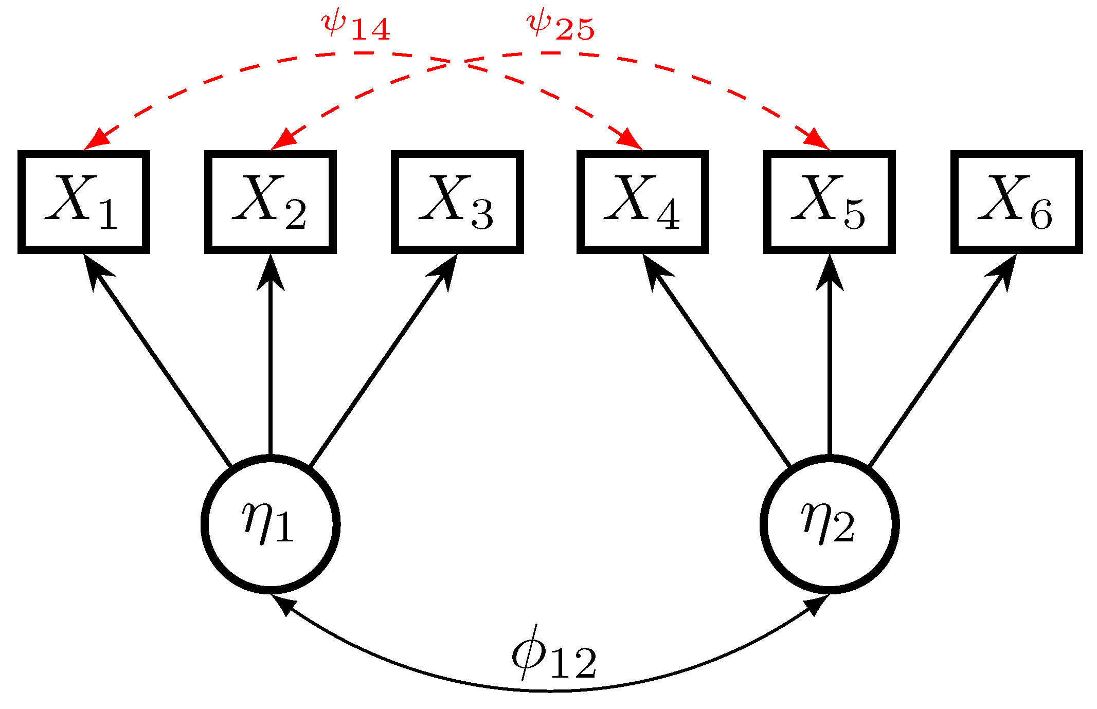
3. Simulation Study 1: Unmodeled Residual Error Correlation

In this Simulation Study 1, we compare the estimation approaches RME and RegML in a misspecified single-group two-dimensional factor model. It is of interest which of the estimation methods is resistant to model misspecification. It can be expected that RegML and RME with powers $p\le 1$ will provide some resistance to model errors.

3.1. Method

The data-generating model is a two-dimensional factor model involving six manifest variables $X_1,\dots ,X_6$, and two latent (factor) variables ${\eta }_1$ and ${\eta }_2$. The data-generating model is graphically presented in Figure 1. The first three items load on the first factor, while the last three item load on the second factor. Model errors exist by introducing two unmodeled residual correlations of items corresponding to the two factors (i.e., of items $X_1$ and $X_4$, and items $X_2$ and $X_5$).

The means of all variables were set to equal in the population. However, the mean structure was left saturated in estimation because it is not of interest in this simulation study. The specified factor loadings $\lambda$ were all set to 0.7, and all error variances were set to 0.5. The latent correlation ${\varphi }_{12}$ of the factors ${\eta }_1$ and ${\eta }_2$ was set to 0.5 in the simulation. The factor variable $\mathbf{\eta }$, as well as the residuals $\mathbf{ϵ}$, were multivariate normally distributed.

We varied the size of both residual error correlations as $0.5·\delta$ with $\delta =0$, 0.3, and 0.6, indicating moderate-sized and large-sized residual error correlations. The sample size N was chosen to 500, 1000, or 2500.

We estimated the two-dimensional factor model with unmodeled residual error correlations. That is, the analysis models were misspecified (except for RegML). The six factor loadings and the six residual variances were freely estimated. The variances of the latent factors were set to 1. We employed ML, ULS, RegML, and RME, utilizing the $L_p$ loss function with powers $p=0.25$, 0.5, and 1. ML and ULS can be considered non-robust SEM estimation approaches, while RegML and RME are considered robust approaches. In total, six different estimates were compared for each simulated dataset in each condition.

For RegML, we only imposed the SCAD penalty on nondiagonal entries in the residual covariance matrix $\mathbf{\Psi }$. RegML was estimated at a grid of regularization parameters between 10 and 0.002 (see replication material on https://osf.io/v8f45 (accessed on 27 March 2023) for specification details). In this simulation study, the tuning parameter a was fixed to 3.7. We chose estimates of the regularization approach using the optimal regularization ${\kappa }_{\mathbf{\psi }}$ based on the BIC.

We studied the estimation recovery of the factor correlation ${\varphi }_{12}$, a factor loading ${\lambda }_{11}$, and a residual variance ${\psi }_{11}$. We assessed the bias and root mean square error (RMSE) of a parameter $\widehat{\theta }$ of interest. In each of $R=2000$ replications in a simulation condition, the estimate ${\widehat{\theta }}_r$ ($r=1,\dots ,R$) was calculated. The bias was estimated by

$$\mathrm{Bias}\left(\widehat{\theta }\right)=\frac{1}{R}\sum _{r=1}^R({\widehat{\theta }}_r-\theta ).$$

(25)

The RMSE was estimated by

$$\mathrm{RMSE}\left(\widehat{\theta }\right)=\frac{1}{R}\sum _{r=1}^R{({\widehat{\theta }}_r-\theta )}^2.$$

(26)

To ease the comparability of the RMSE between different methods across sample sizes, we used a relative RMSE in which we divided the RMSE of a particular method by the RMSE of the best-performing method in a simulation condition. Hence, a relative RMSE of 100 is the reference value for the best-performing method.

The statistical software R [60] was employed for all parts of the simulation. All estimators of the SEM were obtained using the mgsem() function in the sirt [61] package. Replication material can be found at https://osf.io/v8f45 (accessed on 27 March 2023).

3.2. Results

In

Table 1. Simulation Study 1: Bias and relative root mean square error (RMSE) of model parameter estimates as a function of sample size N and size of residual error correlations $\delta$.

			Bias							Relative RMSE
				RME with p =							RME with p =
Par	$\mathit{\delta }$	N	RegML	0.25	0.5	1	ULS	ML		RegML	0.25	0.5	1	ULS	ML
${\varphi }_{12}$	0	500	−0.01	$\phantom{-}$0.00	$\phantom{-}$0.00	$\phantom{-}$0.00	$\phantom{-}$0.00	$\phantom{-}$0.00		102	102	101	101	100	101
		1000	$\phantom{-}$0.00	$\phantom{-}$0.00	$\phantom{-}$0.00	$\phantom{-}$0.00	$\phantom{-}$0.00	$\phantom{-}$0.00		102	101	101	100	100	100
		2500	$\phantom{-}$0.00	$\phantom{-}$0.00	$\phantom{-}$0.00	$\phantom{-}$0.00	$\phantom{-}$0.00	$\phantom{-}$0.00		103	100	100	100	100	100
	0.3	500	$\phantom{-}$0.02	$\phantom{-}$0.02	$\phantom{-}$0.02	$\phantom{-}$0.03	$\phantom{-}$0.07	$\phantom{-}$0.07		100	101	103	113	162	166
		1000	$\phantom{-}$0.01	$\phantom{-}$0.01	$\phantom{-}$0.01	$\phantom{-}$0.03	$\phantom{-}$0.07	$\phantom{-}$0.07		100	101	105	122	213	218
		2500	$\phantom{-}$0.01	$\phantom{-}$0.01	$\phantom{-}$0.01	$\phantom{-}$0.03	$\phantom{-}$0.07	$\phantom{-}$0.07		100	101	108	144	318	328
	0.6	500	$\phantom{-}$0.01	$\phantom{-}$0.01	$\phantom{-}$0.01	$\phantom{-}$0.03	$\phantom{-}$0.15	$\phantom{-}$0.16		100	101	102	119	312	336
		1000	$\phantom{-}$0.00	$\phantom{-}$0.01	$\phantom{-}$0.01	$\phantom{-}$0.03	$\phantom{-}$0.15	$\phantom{-}$0.16		100	100	103	129	429	462
		2500	$\phantom{-}$0.00	$\phantom{-}$0.01	$\phantom{-}$0.01	$\phantom{-}$0.03	$\phantom{-}$0.15	$\phantom{-}$0.16		100	100	105	152	672	722
${\lambda }_{11}$	0	500	$\phantom{-}$0.00	$\phantom{-}$0.00	$\phantom{-}$0.00	$\phantom{-}$0.00	$\phantom{-}$0.00	$\phantom{-}$0.00		101	108	106	104	104	100
		1000	$\phantom{-}$0.00	$\phantom{-}$0.00	$\phantom{-}$0.00	$\phantom{-}$0.00	$\phantom{-}$0.00	$\phantom{-}$0.00		101	105	104	103	104	100
		2500	$\phantom{-}$0.00	$\phantom{-}$0.00	$\phantom{-}$0.00	$\phantom{-}$0.00	$\phantom{-}$0.00	$\phantom{-}$0.00		101	104	104	104	104	100
	0.3	500	$\phantom{-}$0.00	$\phantom{-}$0.00	$\phantom{-}$0.00	$\phantom{-}$0.01	$\phantom{-}$0.02	$\phantom{-}$0.01		102	104	103	101	109	100
		1000	$\phantom{-}$0.00	$\phantom{-}$0.00	$\phantom{-}$0.00	$\phantom{-}$0.01	$\phantom{-}$0.02	$\phantom{-}$0.01		100	101	101	102	117	102
		2500	$\phantom{-}$0.00	$\phantom{-}$0.00	$\phantom{-}$0.00	$\phantom{-}$0.01	$\phantom{-}$0.02	$\phantom{-}$0.01		100	100	101	105	137	108
	0.6	500	$\phantom{-}$0.00	$\phantom{-}$0.00	$\phantom{-}$0.00	$\phantom{-}$0.01	$\phantom{-}$0.04	$\phantom{-}$0.02		100	108	107	107	139	138
		1000	$\phantom{-}$0.00	$\phantom{-}$0.00	$\phantom{-}$0.00	$\phantom{-}$0.01	$\phantom{-}$0.04	$\phantom{-}$0.02		100	107	107	110	166	146
		2500	$\phantom{-}$0.00	$\phantom{-}$0.00	$\phantom{-}$0.00	$\phantom{-}$0.01	$\phantom{-}$0.04	$\phantom{-}$0.02		100	104	105	111	219	160
${\psi }_{11}$	0	500	$\phantom{-}$0.00	$\phantom{-}$0.00	$\phantom{-}$0.00	$\phantom{-}$0.00	$\phantom{-}$0.00	$\phantom{-}$0.00		100	117	113	109	109	100
		1000	$\phantom{-}$0.00	$\phantom{-}$0.00	$\phantom{-}$0.00	$\phantom{-}$0.00	$\phantom{-}$0.00	$\phantom{-}$0.00		100	109	107	106	107	100
		2500	$\phantom{-}$0.00	$\phantom{-}$0.00	$\phantom{-}$0.00	$\phantom{-}$0.00	$\phantom{-}$0.00	$\phantom{-}$0.00		101	107	107	107	108	100
	0.3	500	−0.02	−0.01	−0.01	−0.01	−0.03	−0.02		107	110	107	105	116	100
		1000	−0.01	−0.01	−0.01	−0.01	−0.03	−0.02		104	100	100	103	127	102
		2500	−0.01	$\phantom{-}$0.00	−0.01	−0.01	−0.03	−0.01		107	100	101	108	155	111
	0.6	500	−0.02	$\phantom{-}$0.00	−0.01	−0.01	−0.06	−0.03		105	102	100	100	139	136
		1000	−0.01	$\phantom{-}$0.00	$\phantom{-}$0.00	−0.01	−0.06	−0.03		102	101	100	104	176	145
		2500	$\phantom{-}$0.00	$\phantom{-}$0.00	$\phantom{-}$0.00	−0.01	−0.06	−0.03		100	101	102	112	260	177

Note. Par  = model parameter; ML = maximum likelihood estimate; RegML = regularized maximum likelihood estimate using the Bayesian information criterion for regularization parameter selection; RME  = robust moment estimation with power p in the loss function $\rho \left(x\right)={\left|x\right|}^p$; ULS  = unweighted least squares estimate; Biases with absolute values of at least 0.03 are printed in bold. RMSE values of at least 110 are printed in bold.

, the bias and the relative RMSE for the factor correlation ${\varphi }_{12}$, the factor loading ${\lambda }_{11}$, and the residual variance ${\psi }_{11}$ are presented.

It turned out that in the condition of no unmodeled residual error correlations (i.e., $\delta =0$ and no model misspecification), no biases occurred for all parameters. However, there were slight efficiency losses with RME for $N=500$, which were particularly pronounced for the powers $p=0.25$ and $p=0.5$ for the residual variance. The efficiency loss for the factor loading for the robust estimation methods was slightly smaller than for the residual variance. Finally, there was almost no efficiency loss for the robust methods for the factor correlation.

In the conditions with model errors (i.e., in the case of unmodeled residual correlations), ML and ULS were severely biased for the factor correlation. The bias for ML and ULS turned out to be slightly smaller for the factor loading and the residual variance. RegML and RME, using the powers $p=0.25$ or $p=0.5$, were unbiased, while RME with $p=1$ had a small bias for the latent correlation. Regarding efficiency, RME with $p=0.25$ was superior to $p=0.5$.

In general, RME with $p=0.25$ performed quite competitively to RegML. Given the fact that RMSE is computationally much less demanding than RegML, one could prefer model-robust SEM estimation in the presence of unmodeled residual error correlations using the $L_p$ robust loss function in practical applications.

4. Focused Simulation Study 1A: Computation of Standard Errors

In this Focused Simulation Study 1A, different standard error estimation formulas are compared for selected conditions of Simulation Study 1.

4.1. Method

The same data-generating model of Simulation Study 1 (see Section 3) was utilized in a subset of conditions. Multivariate data was generated based on a two-dimensional factor model with two residual correlations. The correlations were omitted from the analysis model. The size of the residual correlations was chosen as $0.5·\delta$ with $\delta$ equal to 0 or 0.6. The same sample sizes as in Simulation Study 1 were employed (i.e., $N=500$, 1000, and 2500).

The same estimation methods as in Simulation Study 1, except RegML, were used (i.e., ML, ULS, and RME with $p=0.25$, 0.5, and 1). Standard errors were computed for each estimation method based on the multivariate delta formula (DF; see Equation (21)) that is implemented in the sirt::mgsem() function in the R package sirt [61]. Moreover, the resampling methods jackknife (JK) and bootstrap (BS) were used [42,62]. For jackknife, 40 replication zones were employed for determining the standard error of model parameter estimates. For bootstrap, 100 bootstrap samples were used to compute the standard deviation of a parameter estimate across bootstrap samples that were used as the standard error estimate. Moreover, standard errors for ML were also computed based on the observed information (OI) matrix obtained as the Hessian of the log-likelihood function. Note that the OI method is expected to result in biased standard error estimates in misspecified models (i.e., in the case of $\delta =0.6$).

Confidence intervals around model parameter estimates were constructed under a normality assumption of a parameter estimate at a confidence level of 95%. The empirical coverage rate was determined as the proportion that the confidence interval covers the pseudo-true parameter of an estimation method. A corresponding pseudo-true parameter was obtained by applying the respective estimation method to the covariance matrix of observed variables (i.e., $\mathrm{Var}\left(\mathit{X}\right)$) in an infinite sample size (i.e., at the population level).

In total, 4000 replications were used for estimating the coverage rate at the confidence level of 95%. A dedicated function for JK and BS standard error computation was written in R [60]. Model estimation and standard error computation based on DF were carried out using the mgsem() function in the R package sirt [61].

4.2. Results

In

Table 2. Focused Simulation Study 1A: Coverage rate at confidence level 95% of model parameter estimates as a function of sample size N and size of residual error correlations $\delta$ for different standard error estimation methods.

			RME with p =
			0.25				0.5				1				ULS				ML
Par	$\mathit{\delta }$	N	DF	JK	BS		DF	JK	BS		DF	JK	BS		DF	JK	BS		OI	DF	JK	BS
${\varphi }_{12}$	0	500	95.8	95.1	95.5		95.5	94.8	94.9		95.3	94.4	95.0		94.9	94.2	94.6		95.0	95.1	94.2	94.6
		1000	95.2	94.7	94.9		95.1	94.6	94.7		94.8	94.4	94.7		94.6	94.2	94.3		94.7	94.7	94.4	94.5
		2500	95.4	94.7	95.3		95.3	94.7	94.9		95.3	94.6	94.9		95.2	94.7	94.7		95.2	95.2	94.7	94.9
	0.6	500	94.8	94.5	94.6		94.5	94.1	94.5		93.7	93.0	93.3		94.7	94.0	94.3		93.5	94.4	93.7	94.4
		1000	94.3	94.0	94.7		94.3	93.7	94.1		93.7	93.3	93.1		94.7	94.0	94.4		93.6	94.6	94.0	94.1
		2500	95.1	94.5	95.0		95.0	94.3	94.7		95.0	94.2	94.1		95.2	94.5	94.8		94.3	95.2	94.3	94.6
${\lambda }_{11}$	0	500	95.8	95.4	96.0		95.6	95.1	95.9		95.2	94.5	95.1		94.7	94.0	94.3		95.0	95.1	93.9	94.7
		1000	95.2	94.3	95.6		95.1	93.9	95.1		94.6	93.7	94.4		94.4	93.4	93.7		94.6	94.7	93.8	93.8
		2500	94.5	93.8	94.6		94.4	93.8	94.1		94.2	93.9	94.3		94.2	93.8	94.0		94.6	94.6	93.8	94.1
	0.6	500	95.5	94.9	96.0		95.6	94.7	96.2		95.6	94.5	95.3		94.9	93.8	94.5		88.5	96.2	95.7	96.4
		1000	95.1	94.5	95.5		94.9	94.5	95.0		94.7	94.4	94.8		94.6	93.8	94.4		88.5	95.6	94.7	95.9
		2500	95.1	94.7	95.2		95.0	94.7	94.9		95.3	94.5	94.9		95.2	94.3	94.9		89.0	95.4	94.5	95.4
${\psi }_{11}$	0	500	96.6	96.2	97.6		96.4	95.8	96.9		95.8	94.8	95.4		95.1	94.3	94.4		95.0	95.0	94.4	94.9
		1000	96.1	95.3	96.7		95.9	95.1	95.9		95.5	94.8	95.3		95.3	94.6	94.9		95.1	95.1	94.7	94.9
		2500	95.0	94.7	95.3		95.1	94.6	95.1		95.1	94.6	94.9		95.0	94.5	94.7		95.0	95.0	94.3	94.4
	0.6	500	96.1	95.7	97.1		96.1	95.6	96.9		95.7	95.2	95.8		94.9	94.5	94.6		88.7	96.7	96.5	96.8
		1000	95.3	95.0	95.9		95.4	95.0	95.8		95.3	94.7	95.3		94.9	94.2	94.7		88.6	95.8	95.1	96.4
		2500	95.1	94.7	95.0		95.1	94.6	95.0		94.9	94.5	94.8		95.1	94.5	94.7		88.8	95.2	94.8	95.6

Note. Par  = model parameter; ML = maximum likelihood estimate; RegML = regularized maximum likelihood estimate using the Bayesian information criterion for regularization parameter selection; RME  = robust moment estimation with power p in the loss function $\rho \left(x\right)={\left|x\right|}^p$; ULS  = unweighted least squares estimate; DF = standard error estimation based on delta formula; JK = standard error estimation based on jackknife; BS = standard error estimation based on bootstrap; OI = standard error estimation based on observed information.

, coverage rates at the confidence level of 95% of model parameter estimates as a function of sample size N and the size $\delta$ of unmodeled residual error correlations are displayed. Overall, it turned out that DF, JK, and BS standard error estimates resulted in satisfactory coverage rates (i.e., between 92.5% and 97.5%) for a correctly specified (i.e., $\delta =0$) and a misspecified (i.e., $\delta =0.6$) SEM. As expected, standard errors based on the OI resulted in undercoverage for a misspecified SEM. Given the fact that standard error computation based on DF is much less computationally demanding, it can be recommended for usage in RME. Computationally more involved resampling methods, such as JK or BS, are, therefore, not necessarily required.

5. Simulation Study 2: Noninvariant Item Intercepts (DIF)

In this Simulation Study 2, we investigate the impact of unmodelled group-specific item intercepts in a multiple-group one-dimensional factor model. The presence of group-specific item intercepts indicates measurement noninvariance (i.e., in the presence of DIF). This simulation study investigates whether robust estimation approaches can handle the occurrence of DIF.

5.1. Method

The setup of the simulation study closely follows [32]. Data were simulated from a one-dimensional factor model involving five items and three groups. The factor variable ${\eta }_1$ was normally distributed with group means ${\alpha }_1=0$, ${\alpha }_2=0.3$, and ${\alpha }_3=0.8$. The group variances were set to 1, 1.5, and 1.2, respectively. All factor loadings were set to 1, and all measurement error variances were set to 1 in all groups and uncorrelated with each other. The factor variable, as well as the residuals, were normally distributed.

DIF effects were simulated in exactly one of the five items in each group. In the first group, the fourth item intercepts had a DIF effect $\delta$. In the second group, the first item had a DIF effect $-\delta$, while the second item had a DIF effect $-\delta$ in the third group. The DIF effect $\delta$ was chosen as either 0 (no DIF, measurement invariance), 0.3 (small DIF), or 0.6 (moderate DIF). The sample size per group was chosen as $N=500$, 1000, or 2000.

A multiple-group one-dimensional SEM was specified as the analysis model. The analysis model assumes invariant item intercepts and factor loadings. In the first group, the factor mean was set to 0, and the factor variance was set to 1 for identification reasons. Note that the data-generating model included some group-specific item intercepts that remained unmodelled in the analysis models (except for RegML). This, in turn, led to misspecified analysis models. ML, ULS, RegML with the SCAD penalty on group-specific item intercepts, and RME with powers $p=0.25$, 0.5, and 1 were utilized. In RegML, the optimal regularization parameter ${\kappa }_{\mathbf{\nu }}$ was chosen based on the BIC.

We investigated the estimation recovery of group means ${\alpha }_2$ and ${\alpha }_3$ of the second and the third group, respectively. Bias and relative RMSE (see Section 3.1) were again used for assessing the performance of the estimates. In total, 2000 replications were conducted. The models were estimated using the mgsem() function in the R [60] package sirt [61]. Replication material can be found at https://osf.io/v8f45 (accessed on 27 March 2023).

5.2. Results

In

Table 3. Simulation Study 2: Bias and relative root mean square error (RMSE) of model parameter estimates as a function of sample size N and size of DIF effects $\delta$.

			Bias							Relative RMSE
				RME with p =							RME with p =
Par	$\mathit{\delta }$	N	RegML	0.25	0.5	1	ULS	ML		RegML	0.25	0.5	1	ULS	ML
${\alpha }_2$	0	500	$\phantom{-}$0.00	$\phantom{-}$0.00	$\phantom{-}$0.00	$\phantom{-}$0.00	$\phantom{-}$0.00	$\phantom{-}$0.00		100	103	102	100	100	100
		1000	$\phantom{-}$0.00	$\phantom{-}$0.00	$\phantom{-}$0.00	$\phantom{-}$0.00	$\phantom{-}$0.00	$\phantom{-}$0.00		100	102	101	100	100	100
		2500	$\phantom{-}$0.00	$\phantom{-}$0.00	$\phantom{-}$0.00	$\phantom{-}$0.00	$\phantom{-}$0.00	$\phantom{-}$0.00		100	100	100	100	100	100
	0.3	500	−0.02	−0.03	−0.03	−0.07	−0.12	−0.12		101	100	100	113	152	152
		1000	$\phantom{-}$0.00	−0.01	−0.02	−0.06	−0.12	−0.12		100	103	106	140	231	230
		2500	$\phantom{-}$0.00	−0.01	−0.01	−0.05	−0.12	−0.12		100	103	107	169	356	355
	0.6	500	$\phantom{-}$0.00	−0.01	−0.02	−0.07	−0.24	−0.24		100	104	104	129	303	302
		1000	$\phantom{-}$0.00	−0.01	−0.01	−0.06	−0.24	−0.24		100	102	103	144	435	433
		2500	$\phantom{-}$0.00	$\phantom{-}$0.00	−0.01	−0.05	−0.24	−0.24		100	101	104	171	698	692
${\alpha }_3$	0	500	$\phantom{-}$0.01	$\phantom{-}$0.01	$\phantom{-}$0.01	$\phantom{-}$0.01	$\phantom{-}$0.01	$\phantom{-}$0.01		100	103	102	101	100	100
		1000	$\phantom{-}$0.00	$\phantom{-}$0.00	$\phantom{-}$0.00	$\phantom{-}$0.00	$\phantom{-}$0.00	$\phantom{-}$0.00		100	102	101	100	100	100
		2500	$\phantom{-}$0.00	$\phantom{-}$0.00	$\phantom{-}$0.00	$\phantom{-}$0.00	$\phantom{-}$0.00	$\phantom{-}$0.00		100	101	101	100	100	100
	0.3	500	−0.02	−0.03	−0.03	−0.07	−0.12	−0.11		100	103	102	115	153	149
		1000	$\phantom{-}$0.00	−0.01	−0.02	−0.06	−0.12	−0.11		100	104	107	139	223	216
		2500	$\phantom{-}$0.00	−0.01	−0.01	−0.05	−0.12	−0.12		100	103	108	167	344	332
	0.6	500	$\phantom{-}$0.00	−0.01	−0.01	−0.06	−0.23	−0.21		100	103	102	124	286	267
		1000	$\phantom{-}$0.00	$\phantom{-}$0.00	−0.01	−0.05	−0.23	−0.22		100	103	103	139	421	390
		2500	$\phantom{-}$0.00	−0.01	−0.01	−0.05	−0.24	−0.22		100	101	104	174	693	641

Note. Par  = model parameter; ML = maximum likelihood estimate; RegML = regularized maximum likelihood estimate using the Bayesian information criterion for regularization parameter selection; RME  = robust moment estimation with power p in the loss function $\rho \left(x\right)={\left|x\right|}^p$; ULS  = unweighted least squares estimate; Biases with absolute values of at least 0.03 are printed in bold. RMSE values of at least 110 are printed in bold.

, bias and relative RMSE for the factor means of the second and the third group (i.e., ${\alpha }_2$ and ${\alpha }_3$) are presented.

In the condition of no DIF effects (i.e., $\delta =0$), all different estimators were unbiased. There were minor efficiency losses for robust moment estimation with $p=0.25$ and $p=0.5$ for the sample size $N=500$. However, in larger samples, there were almost no differences among the different estimators.

In the simulation conditions with small or moderate DIF effects, ML and ULS were substantially biased. Notably, RME with $p=1$ also produced a nonnegligible bias. RME with powers $p=0.25$ or $p=0.5$ performed similarly to RegML concerning bias. RME had only slightly increased efficiency losses. Interestingly, RME $p=0.25$ performed better than $p=0.5$ in terms of RMSE.

Given the fact that there were only small efficiency losses with RME, the computationally more expensive RegML could perhaps be avoided in practice if the goal is estimating factor group means.

6. Empirical Example: ESS 2005 Data

We now present an empirical example to illustrate the performance of the different robust and non-robust SEM estimation approaches.

6.1. Method

In this empirical example, we use a dataset that was also analyzed in [32,63,64]. The data came from the European social survey (ESS) conducted in the year 2005 (ESS 2005) including subjects from 26 countries. The latent factor variable of tradition and conformity was assessed by four items presented in portrait format, where the scale of the items is such that a high value represents a low level of tradition conformity. The wording of the four items was (see [32]): “It is important for him to be humble and modest. He tries not to draw attention to himself.” (item TR9), “Tradition is important to him. He tries to follow the customs handed down by his religion or family.” (item TR20), “He believes that people should do what they’re told. He thinks people should follow rules at all times, even when no one is watching.” (item CO7), and “It is important for him to always behave properly. He wants to avoid doing anything people would say is wrong.” (item CO16). The full dataset used in [32] was downloaded from https://www.statmodel.com/Alignment.shtml (accessed on 27 March 2023). For this empirical example, a subsample of 33,060 persons from 17 selected countries was included to restrict the range of variability of country factor means. The sample sizes per country ranged between 1358 and 2963, with an average of 1997.1 ($\mathrm{SD}=464.5$). We only included participants in the sample that had no missing values on all four items.

We specified a one-dimensional factor model with 17 groups (i.e., 17 countries) assuming invariant item parameters (i.e., invariant intercepts, loadings, and residual variances) in the estimation approaches ML, ULS, and RME, with powers $p=0.25$, 0.5, and 1. In RegML, the SCAD penalty was imposed on group-specific item intercepts.

The obtained country means and country standard deviations of the factor variable were linearly transformed for all different estimators such that the total population comprising all persons from all 17 countries had a mean of 0 and a standard deviation of 1.

The analysis was conducted using the mgsem() function from the R [60] package sirt [61]. The processed dataset and replication syntax can be found at https://osf.io/v8f45 (accessed on 27 March 2023).

6.2. Results

In the following, we present the estimates of RegML with the obtained optimal regularization parameter ${\kappa }_{\nu }$ of 0.02.

In

Table 4. Empirical example: Estimated country means for different estimation methods.

			RME with p =
Rank	CNT	RegML	0.25	0.5	1	ULS	ML
1	C10	0.37	0.37	0.37	0.34	0.34	0.35
2	C21	0.01	−0.01	0.01	0.18	0.27	0.33
3	C06	0.06	0.17	0.19	0.26	0.25	0.26
4	C03	0.33	0.33	0.32	0.25	0.21	0.21
5	C08	0.13	0.15	0.16	0.23	0.23	0.20
6	C12	0.12	0.14	0.15	0.20	0.19	0.16
7	C05	0.15	0.17	0.17	0.15	0.11	0.13
8	C16	0.14	0.05	0.06	0.09	0.06	0.07
9	C01	0.12	0.11	0.10	0.07	0.08	0.07
10	C14	−0.11	−0.10	−0.10	−0.09	−0.05	−0.06
11	C22	0.02	−0.01	−0.02	−0.06	−0.08	−0.07
12	C15	−0.18	−0.17	−0.17	−0.16	−0.01	−0.07
13	C09	−0.21	−0.21	−0.21	−0.21	−0.19	−0.23
14	C13	−0.30	−0.30	−0.30	−0.32	−0.28	−0.30
15	C17	−0.20	−0.19	−0.21	−0.29	−0.36	−0.33
16	C25	−0.17	−0.18	−0.19	−0.29	−0.39	−0.34
17	C24	−0.29	−0.32	−0.34	−0.37	−0.38	−0.39

Note. Rank = country rank based on estimated country mean with ML; CNT = country labels originally used in [32]; ML = maximum likelihood estimate; RegML = regularized maximum likelihood estimate using the Bayesian information criterion for regularization parameter selection; RME = robust moment estimation with power p in the loss function $\rho \left(x\right)={\left|x\right|}^p$; ULS = unweighted least squares estimate.

, the country means for the six different estimators are presented. The maximum absolute difference between country means stemming from the different models ranged between 0.032 and 0.337, with an average of 0.116 ($\mathrm{SD}=0.081$). This showed considerable variability. Hence, the different robust and non-robust estimators differently weighted DIF effects in the computation of country means.

We also computed the ranks of the 17 countries across the six different estimates. The maximum absolute country rank difference ranged between 0 (country C10, rank 1) and 8 (country C21, rank 2) with an average of 3.9 ($\mathrm{SD}=2.1$). A large range for country means was observed for country C21 (rank 2). The means for this country ranged between −0.01 (RME) and 0.33 (ML). Note that robust approaches provided similar results, but they substantially differed from RME with $p=1$, ULS, and ML. Similarly, for country C06 (rank 3), there was a range of country means with values between 0.06 and 0.26. However, low dependencies of country means from the model estimator choice were observed for countries C10 (rank1), C09 (rank 13), and C13 (rank 14).

In Figure 2, average absolute differences in country means between different models are displayed. Large absolute differences are displayed in darker red-brown color, while small differences are colored in light yellow-orange. RME with $p=0.25$ (i.e., RME0.25) and RME with $p=0.5$ (i.e., “RME0.5”) provided similar country means with an average distance of 0.01. Notably, RegML also resulted in similar estimates to RME, with $p=0.25$ or $p=0.5$ (i.e., average distances of 0.02 or 0.03). In addition, ML and ULS resulted in similar estimates. Interestingly, RME with $p=1$ performed slightly differently compared to the other approaches. As in the simulation studies, it did not show full robustness to outlying DIF effects in item intercepts.

In Figure 3, the regularization paths of the estimated country means as a function of the regularization parameter ${\kappa }_{\mathbf{\nu }}$ are displayed. The RegML estimates of the country means are displayed on the left side of the figure, and the ML estimates are displayed on the right side of the figure. Interestingly, the paths are not monotone, and there is some variability in country mean estimates depending on the choice of the regularization parameter.

In

Table 5. Empirical example: Estimated country-specific item intercepts for regularized maximum likelihood estimation based on BIC regularization parameter selection.

CNT	TR09	TR20	CO07	CO16
C01	·	−0.17	·	−0.17
C03	·	−0.32	·	−0.26
C05	−0.50	0.29	·	·
C06	0.09	·	0.24	·
C08	·	0.12	·	·
C09	·	−0.24	·	0.09
C10	−0.47	0.25	·	·
C12	·	0.05	·	·
C13	0.29	·	·	−0.47
C14	0.10	0.31	·	−0.42
C15	0.42	0.07	·	−0.22
C16	−0.26	·	·	−0.13
C17	−0.52	−0.12	·	·
C21	·	·	0.48	·
C22	−0.14	·	·	−0.36
C24	·	−0.32	·	−0.17
C25	−0.52	·	·	−0.31

Note. CNT = country labels originally used in [32]. Regularized item intercepts are indicated with a dot (i.e., with “·”).

, the estimated country-specific item intercepts for regularized ML estimation are presented. Overall, three countries had three regularized item intercepts, 12 countries had two regularized item intercepts, and two countries had one regularized item intercept. In total, 35 out of 68 item intercepts were regularized (i.e., the country-specific item intercepts were estimated as zero).

The regularization paths for country-specific item intercepts for four selected countries, C01, C09, C13, and C21, are displayed in Figure 4. One immediately recognizes that more and stronger deviations from invariance were observed with smaller values of the regularization parameter ${\kappa }_{\mathbf{\nu }}$.

7. Discussion

In this article, we have demonstrated that, using model-robust SEM estimation methods, such as regularized maximum likelihood estimation and robust moment estimation, provides some resistance to model errors for modeled means and covariances. Importantly, this robustness property is only guaranteed if model errors are sparsely distributed. That is, most of the model errors are zero (or approximately zero), while only a few model errors are allowed to differ from zero. The plausibility of this assumption should be evaluated for each empirical application that potentially involves model error. Moreover it is noted that robust moment SEM estimation approaches did not result in practically relevant efficiency losses compared to non-robust approaches (i.e., maximum likelihood or unweighted least squares estimation) in the absence of model errors. Hence, robust estimation approaches can be recommended in empirical applications with moderate to large sample sizes (i.e., $N\ge 500$). Importantly, robust moment estimation is computationally much less demanding than regularized estimation. Moreover, it also provides valid standard errors that are much more difficult to obtain with regularized ML estimation.

We applied robust moment estimation and regularized ML estimation for unmodeled item intercepts in Simulation Study 2 in Section 5. In this case, there is essentially no need to utilize the more computationally expensive regularization technique. The crucial assumption is that there are only a few model deviations in the modeled mean vectors and covariance matrices. This property is also referred to as the sparsity assumption [51], which means that the majority of the entries in mean vectors and covariance matrices are correctly specified. The methods discussed in this article will typically fail if the majority of or all the elements in the mean vectors and covariance matrices are misspecified [65,66]. This will likely be the case if the item loadings in the confirmatory factor model vary across groups. This situation is referred to as nonuniform DIF. Model deviations in item loadings lead to model deviations in the covariance matrix that is not as sparse as deviations in the mean structure. Hence, this is a situation in which regularized ML estimation might be preferred over robust moment estimation.

The treatment in this article was based on the multivariate normal distribution utilizing mean vectors and covariance matrices as sufficient statistics. Sometimes, researchers tend to model ordinal items by relying on underlying latent normally distributed variables [67,68]. In this case, thresholds and polychoric correlations replace mean vectors and covariance matrices in the weighted least squares fitting function. The approach based on model-robust fitting function can also be simply transferred to the case of modeling ordinal items. Future research might compare the performance of robust moment estimation with limited information methods relying on thresholds and polychoric correlations with regularized maximum likelihood estimation. Clearly, the computational advantages of model-robust limited information methods would be even more pronounced compared to the case of continuous items.

It should be noted that multivariate normality is not a requirement for obtaining consistent estimates in correctly specified structural equation models [37]. This article investigates the robustness of parameter estimates regarding model misspecification in the mean and the covariance structure. There is a distinct literature that focuses on robust estimation of SEM in the violation of multivariate normality [69,70]. These approaches might result in more efficient estimates in the case of heavy-tailed or contaminated distributions. However, outliers in this article are defined in the sense that some entries of the mean vector and the covariance matrix are misspecified infinite sample sizes (i.e., at the population level).

As pointed out in this article, the multiple-group SEM with unmodeled item intercepts corresponds to the estimation in the violation of measurement invariance (i.e., in the presence of differential item functioning). Linking approaches, such as invariance alignment [32,71] or robust Haberman linking [30], also deal with the estimation of factor means in one- or multidimensional confirmatory factor models. They do so by first estimating model parameters of the factor model separately in each group in the first step. In the second step, group-specific estimated item intercepts and factor loadings are transformed with a robust or non-robust linking function to identify factor means and factor standard deviations. This approach is advantageous if there is a misfit in the mean and the covariance structure. If the covariance structure is correctly specified, a joint robust moment estimation approach of the multiple-group SEM could have higher efficiency. In practical applications, it has been shown that misspecification more frequently occurs in the mean structure than in the covariance structure [72]. Hence, the robust moment estimation approach proposed in this article might be a viable alternative to the frequently employed invariance alignment technique. Future research could thoroughly compare robust moment estimation with invariance alignment or robust Haberman linking.

It has been argued that regularized estimation could also be applied with a fixed tuning parameter [73]. Recent research indicated that model parameter estimation could improve when using a fixed tuning parameter instead of an optimal tuning parameter based on the minimal information criterion [20]. Notably, regularized estimation in SEM is also referred to as penalized estimation [74]. In this framework, the penalty function $\mathcal{P}\left(x\right)\propto {\left|x\right|}^{1/2}$ is interpreted as a fixed prior distribution that has a density $f\left(x\right)\propto exp(-|x{|}^{1/2})$ [74] using the so-called alignment loss function (see [30,32]).

An anonymous reviewer also suggested investigating the Huber loss function [10,38] in addition to the $L_p$ power loss function $\rho \left(x\right)={\left|x\right|}^p$ ($p\le 1$). As a disadvantage, the Huber loss function requires an additional tuning parameter. We have some limited empirical experience in using the Huber loss for robust Haberman linking [30]. In this situation, the Huber loss function performed in an inferior way to the $L_p$ loss function. This was particularly the case for asymmetrically distributed (i.e., asymmetrically structured) model deviations. Studying a wider range of robust loss functions in multiple-group SEM might be an interesting topic for future research, although we are somewhat skeptical that the Huber loss function will outperform the $L_p$ loss function in the conditions of our simulation studies.

Finally, it is always a substantive question of whether model errors are allowed to have outliers or not [75]. That is, should statistical models automatically remove particular means or covariances for estimating the parameter $\mathbf{\theta }$? We attacked such a mechanistic approach to model estimation and argued that model deviations, such as violations of measurement invariance, should not automatically result in model refinement [76]. Hence, we do not think that there is always an optimal loss function in every application [75]. If this were true, the statistical inference would always be based on maximum likelihood estimation. However, we believe that researchers intentionally choose a statistical parameter of interest and apply M-estimation theory [77] for the statistical inference that is not based on correctly specified models. In this sense, SEMs can be estimated with non-robust estimation approaches (such as maximum likelihood or unweighted least squares estimation) using an intentionally misspecified model [78,79]. Appearing model errors can be included as additional uncertainty in standard errors of the estimated $\mathbf{\theta }$ parameter. In SEM, ref. [9] proposed such an approach by imposing a stochastic model for model errors. We think that this approach should deserve more attention in empirical research.

References

1. Bartholomew, D.J.; Knott, M.; Moustaki, I. Latent Variable Models and Factor Analysis: A Unified Approach; Wiley: New York, NY, USA, 2011. [Google Scholar] [CrossRef]
2. Bollen, K.A. Structural Equations with Latent Variables; John Wiley & Sons: New York, NY, USA, 1989. [Google Scholar] [CrossRef]
3. Browne, M.W.; Arminger, G. Specification and estimation of mean-and covariance-structure models. In Handbook of Statistical Modeling for the Social and Behavioral Sciences; Arminger, G., Clogg, C.C., Sobel, M.E., Eds.; Springer: Boston, MA, USA, 1995; pp. 185–249. [Google Scholar] [CrossRef]
4. Jöreskog, K.G.; Olsson, U.H.; Wallentin, F.Y. Multivariate Analysis with LISREL; Springer: Basel, Switzerland, 2016. [Google Scholar] [CrossRef]
5. Mulaik, S.A. Foundations of Factor Analysis; CRC Press: Boca Raton, FL, USA, 2009. [Google Scholar] [CrossRef]
6. Shapiro, A. Statistical inference of covariance structures. In Current Topics in the Theory and Application of Latent Variable Models; Edwards, M.C., MacCallum, R.C., Eds.; Routledge: London, UK, 2012; pp. 222–240. [Google Scholar] [CrossRef]
7. Yuan, K.H.; Bentler, P.M. Structural equation modeling. In Handbook of Statistics, Vol. 26: Psychometrics; Rao, C.R., Sinharay, S., Eds.; Elsevier: Amsterdam, The Netherlands, 2007; Volume 26, pp. 297–358. [Google Scholar] [CrossRef]
8. Robitzsch, A. Comparing the robustness of the structural after measurement (SAM) approach to structural equation modeling (SEM) against local model misspecifications with alternative estimation approaches. Stats 2022, 5, 631–672. [Google Scholar] [CrossRef]
9. Wu, H.; Browne, M.W. Quantifying adventitious error in a covariance structure as a random effect. Psychometrika 2015, 80, 571–600. [Google Scholar] [CrossRef] [PubMed]
10. Huber, P.J.; Ronchetti, E.M. Robust Statistics; Wiley: New York, NY, USA, 2009. [Google Scholar] [CrossRef]
11. Maronna, R.A.; Martin, R.D.; Yohai, V.J. Robust Statistics: Theory and Methods; Wiley: New York, NY, USA, 2006. [Google Scholar] [CrossRef]
12. Ronchetti, E. The main contributions of robust statistics to statistical science and a new challenge. Metron 2021, 79, 127–135. [Google Scholar] [CrossRef]
13. Robitzsch, A. Estimation methods of the multiple-group one-dimensional factor model: Implied identification constraints in the violation of measurement invariance. Axioms 2022, 11, 119. [Google Scholar] [CrossRef]
14. Leitgöb, H.; Seddig, D.; Asparouhov, T.; Behr, D.; Davidov, E.; De Roover, K.; Jak, S.; Meitinger, K.; Menold, N.; Muthén, B.; et al. Measurement invariance in the social sciences: Historical development, methodological challenges, state of the art, and future perspectives. Soc. Sci. Res. 2023, 110, 102805. [Google Scholar] [CrossRef]
15. Meredith, W. Measurement invariance, factor analysis and factorial invariance. Psychometrika 1993, 58, 525–543. [Google Scholar] [CrossRef]
16. Millsap, R.E. Statistical Approaches to Measurement Invariance; Routledge: New York, NY, USA, 2011. [Google Scholar] [CrossRef]
17. Holland, P.W.; Wainer, H. (Eds.) Differential Item Functioning: Theory and Practice; Lawrence Erlbaum: Hillsdale, NJ, USA, 1993. [Google Scholar] [CrossRef]
18. Penfield, R.D.; Camilli, G. Differential item functioning and item bias. In Handbook of Statistics, Vol. 26: Psychometrics; Rao, C.R., Sinharay, S., Eds.; Elsevier: Amsterdam, The Netherlands, 2007; pp. 125–167. [Google Scholar] [CrossRef]
19. Chen, Y.; Li, C.; Xu, G. DIF statistical inference and detection without knowing anchoring items. arXiv 2021, arXiv:2110.11112. [Google Scholar]
20. Robitzsch, A. Comparing robust linking and regularized estimation for linking two groups in the 1PL and 2PL models in the presence of sparse uniform differential item functioning. Stats 2023, 6, 192–208. [Google Scholar] [CrossRef]
21. Wang, W.; Liu, Y.; Liu, H. Testing differential item functioning without predefined anchor items using robust regression. J. Educ. Behav. Stat. 2022, 47, 666–692. [Google Scholar] [CrossRef]
22. Boos, D.D.; Stefanski, L.A. Essential Statistical Inference; Springer: New York, NY, USA, 2013. [Google Scholar] [CrossRef]
23. Kolenikov, S. Biases of parameter estimates in misspecified structural equation models. Sociol. Methodol. 2011, 41, 119–157. [Google Scholar] [CrossRef]
24. White, H. Maximum likelihood estimation of misspecified models. Econometrica 1982, 50, 1–25. [Google Scholar] [CrossRef]
25. Browne, M.W. Generalized least squares estimators in the analysis of covariance structures. S. Afr. Stat. J. 1974, 8, 1–24. [Google Scholar] [CrossRef]
26. Savalei, V. Understanding robust corrections in structural equation modeling. Struct. Equ. Model. 2014, 21, 149–160. [Google Scholar] [CrossRef]
27. MacCallum, R.C.; Browne, M.W.; Cai, L. Factor analysis models as approximations. In Factor Analysis at 100; Cudeck, R., MacCallum, R.C., Eds.; Lawrence Erlbaum: Hillsdale, NJ, USA, 2007; pp. 153–175. [Google Scholar] [CrossRef]
28. Siemsen, E.; Bollen, K.A. Least absolute deviation estimation in structural equation modeling. Sociol. Methods Res. 2007, 36, 227–265. [Google Scholar] [CrossRef]
29. van Kesteren, E.J.; Oberski, D.L. Flexible extensions to structural equation models using computation graphs. Struct. Equ. Model. 2022, 29, 233–247. [Google Scholar] [CrossRef]
30. Robitzsch, A. Lp loss functions in invariance alignment and Haberman linking with few or many groups. Stats 2020, 3, 246–283. [Google Scholar] [CrossRef]
31. Kolen, M.J.; Brennan, R.L. Test Equating, Scaling, and Linking; Springer: New York, NY, USA, 2014. [Google Scholar] [CrossRef]
32. Asparouhov, T.; Muthén, B. Multiple-group factor analysis alignment. Struct. Equ. Model. 2014, 21, 495–508. [Google Scholar] [CrossRef]
33. Muthén, B.; Asparouhov, T. IRT studies of many groups: The alignment method. Front. Psychol. 2014, 5, 978. [Google Scholar] [CrossRef]
34. Pokropek, A.; Lüdtke, O.; Robitzsch, A. An extension of the invariance alignment method for scale linking. Psych. Test Assess. Model. 2020, 62, 303–334. [Google Scholar]
35. Battauz, M. Regularized estimation of the nominal response model. Multivar. Behav. Res. 2020, 55, 811–824. [Google Scholar] [CrossRef]
36. Oelker, M.R.; Tutz, G. A uniform framework for the combination of penalties in generalized structured models. Adv. Data Anal. Classif. 2017, 11, 97–120. [Google Scholar] [CrossRef]
37. Shapiro, A. Statistical inference of moment structures. In Handbook of Latent Variable and Related Models; Lee, S.Y., Ed.; Elsevier: Amsterdam, The Netherlands, 2007; pp. 229–260. [Google Scholar] [CrossRef]
38. Fox, J.; Weisberg, S. Robust Regression in R: An Appendix to an R Companion to Applied Regression. 2010. Available online: https://bit.ly/3canwcw (accessed on 27 March 2023).
39. Holland, P.W.; Welsch, R.E. Robust regression using iteratively reweighted least-squares. Commun. Stat. Theory Methods 1977, 6, 813–827. [Google Scholar] [CrossRef]
40. Chatterjee, S.; Mächler, M. Robust regression: A weighted least squares approach. Commun. Stat. Theory Methods 1997, 26, 1381–1394. [Google Scholar] [CrossRef]
41. Ver Hoef, J.M. Who invented the delta method? Am. Stat. 2012, 66, 124–127. [Google Scholar] [CrossRef]
42. Kolenikov, S. Resampling variance estimation for complex survey data. Stata J. 2010, 10, 165–199. [Google Scholar] [CrossRef]
43. Chen, J. Partially confirmatory approach to factor analysis with Bayesian learning: A LAWBL tutorial. Struct. Equ. Model. 2022, 22, 800–816. [Google Scholar] [CrossRef]
44. Geminiani, E.; Marra, G.; Moustaki, I. Single- and multiple-group penalized factor analysis: A trust-region algorithm approach with integrated automatic multiple tuning parameter selection. Psychometrika 2021, 86, 65–95. [Google Scholar] [CrossRef]
45. Hirose, K.; Terada, Y. Sparse and simple structure estimation via prenet penalization. Psychometrika 2022. [Google Scholar] [CrossRef]
46. Huang, P.H.; Chen, H.; Weng, L.J. A penalized likelihood method for structural equation modeling. Psychometrika 2017, 82, 329–354. [Google Scholar] [CrossRef]
47. Huang, P.H. lslx: Semi-confirmatory structural equation modeling via penalized likelihood. J. Stat. Softw. 2020, 93, 1–37. [Google Scholar] [CrossRef]
48. Jacobucci, R.; Grimm, K.J.; McArdle, J.J. Regularized structural equation modeling. Struct. Equ. Model. 2016, 23, 555–566. [Google Scholar] [CrossRef] [PubMed]
49. Li, X.; Jacobucci, R.; Ammerman, B.A. Tutorial on the use of the regsem package in R. Psych 2021, 3, 579–592. [Google Scholar] [CrossRef]
50. Scharf, F.; Nestler, S. Should regularization replace simple structure rotation in exploratory factor analysis? Struct. Equ. Model. 2019, 26, 576–590. [Google Scholar] [CrossRef]
51. Fan, J.; Li, R.; Zhang, C.H.; Zou, H. Statistical Foundations of Data Science; Chapman and Hall/CRC: Boca Raton, FL, USA, 2020. [Google Scholar] [CrossRef]
52. Hastie, T.; Tibshirani, R.; Wainwright, M. Statistical Learning with Sparsity: The Lasso and Generalizations; CRC Press: Boca Raton, FL, USA, 2015. [Google Scholar] [CrossRef]
53. Friedrich, S.; Groll, A.; Ickstadt, K.; Kneib, T.; Pauly, M.; Rahnenführer, J.; Friede, T. Regularization approaches in clinical biostatistics: A review of methods and their applications. Stat. Methods Med. Res. 2023, 32, 425–440. [Google Scholar] [CrossRef] [PubMed]
54. Fan, J.; Li, R. Variable selection via nonconcave penalized likelihood and its oracle properties. J. Am. Stat. Assoc. 2001, 96, 1348–1360. [Google Scholar] [CrossRef]
55. Chen, Y.; Liu, J.; Xu, G.; Ying, Z. Statistical analysis of Q-matrix based diagnostic classification models. J. Am. Stat. Assoc. 2015, 110, 850–866. [Google Scholar] [CrossRef]
56. Zhang, H.; Li, S.J.; Zhang, H.; Yang, Z.Y.; Ren, Y.Q.; Xia, L.Y.; Liang, Y. Meta-analysis based on nonconvex regularization. Sci. Rep. 2020, 10, 5755. [Google Scholar] [CrossRef]
57. Tutz, G.; Gertheiss, J. Regularized regression for categorical data. Stat. Model. 2016, 16, 161–200. [Google Scholar] [CrossRef]
58. Kyung, M.; Gill, J.; Ghosh, M.; Casella, G. Penalized regression, standard errors, and Bayesian lassos. Bayesian Anal. 2010, 5, 369–411. [Google Scholar] [CrossRef]
59. Minnier, J.; Tian, L.; Cai, T. A perturbation method for inference on regularized regression estimates. J. Am. Stat. Assoc. 2011, 106, 1371–1382. [Google Scholar] [CrossRef]
60. R Core Team. R: A Language and Environment for Statistical Computing; R Foundation for Statistical Computing: Vienna, Austria, 2022; Available online: https://www.R-project.org/ (accessed on 11 January 2022).
61. Robitzsch, A. sirt: Supplementary Item Response Theory Models; R Package Version 3.13-128. 2023. Available online: https://github.com/alexanderrobitzsch/sirt (accessed on 2 April 2023).
62. Efron, B.; Tibshirani, R.J. An Introduction to the Bootstrap; CRC Press: Boca Raton, FL, USA, 1994. [Google Scholar] [CrossRef]
63. Knoppen, D.; Saris, W. Do we have to combine values in the Schwartz’ human values scale? A comment on the Davidov studies. Surv. Res. Methods 2009, 3, 91–103. [Google Scholar] [CrossRef]
64. Beierlein, C.; Davidov, E.; Schmidt, P.; Schwartz, S.H.; Rammstedt, B. Testing the discriminant validity of Schwartz’ portrait value questionnaire items—A replication and extension of Knoppen and Saris (2009). Surv. Res. Methods 2012, 6, 25–36. [Google Scholar] [CrossRef]
65. Muthén, B.; Asparouhov, T. New Methods for the Study of Measurement Invariance with Many Groups. Technical Report. 2013. Available online: https://bit.ly/3nBbr5M (accessed on 4 March 2023).
66. Muthén, B.; Asparouhov, T. Recent methods for the study of measurement invariance with many groups: Alignment and random effects. Sociol. Methods Res. 2018, 47, 637–664. [Google Scholar] [CrossRef]
67. Muthén, B. A general structural equation model with dichotomous, ordered categorical, and continuous latent variable indicators. Psychometrika 1984, 49, 115–132. [Google Scholar] [CrossRef]
68. Robitzsch, A. On the bias in confirmatory factor analysis when treating discrete variables as ordinal instead of continuous. Axioms 2022, 11, 162. [Google Scholar] [CrossRef]
69. Yuan, K.H.; Bentler, P.M.; Chan, W. Structural equation modeling with heavy tailed distributions. Psychometrika 2004, 69, 421–436. [Google Scholar] [CrossRef]
70. Yuan, K.H.; Bentler, P.M. Robust procedures in structural equation modeling. In Handbook of Latent Variable and Related Models; Lee, S.Y., Ed.; Elsevier: Amsterdam, The Netherlands, 2007; pp. 367–397. [Google Scholar] [CrossRef]
71. Pokropek, A.; Davidov, E.; Schmidt, P. A Monte Carlo simulation study to assess the appropriateness of traditional and newer approaches to test for measurement invariance. Struct. Equ. Model. 2019, 26, 724–744. [Google Scholar] [CrossRef]
72. Rutkowski, L.; Svetina, D. Assessing the hypothesis of measurement invariance in the context of large-scale international surveys. Educ. Psychol. Meas. 2014, 74, 31–57. [Google Scholar] [CrossRef]
73. Liu, X.; Wallin, G.; Chen, Y.; Moustaki, I. Rotation to sparse loadings using Lp losses and related inference problems. Psychometrika 2023. [Google Scholar] [CrossRef]
74. Asparouhov, T.; Muthén, B. Penalized Structural Equation Models. Technical Report. 2023. Available online: https://bit.ly/3TlbxdC (accessed on 4 March 2023).
75. Hennig, C.; Kutlukaya, M. Some thoughts about the design of loss functions. Revstat Stat. J. 2007, 5, 19–39. [Google Scholar] [CrossRef]
76. Robitzsch, A.; Lüdtke, O. Why full, partial, or approximate measurement invariance are not a prerequisite for meaningful and valid group comparisons. Struct. Equ. Model. 2023. [Google Scholar]
77. Stefanski, L.A.; Boos, D.D. The calculus of M-estimation. Am. Stat. 2002, 56, 29–38. [Google Scholar] [CrossRef]
78. Hennig, C. How wrong models become useful-and correct models become dangerous. In Between Data Science and Applied Data Analysis. Studies in Classification, Data Analysis, and Knowledge Organization; Schader, M., Gaul, W., Vichi, M., Eds.; Springer: Berlin, Germany, 2003; pp. 235–243. [Google Scholar] [CrossRef]
79. Saltelli, A.; Funtowicz, S. When all models are wrong. Issues Sci. Technol. 2014, 30, 79–85. [Google Scholar]
Figure 1. Simulation Study 1: Data-generating model.
Algorithms 16 00210 g001
Figure 2. Empirical example: Visualization of average absolute deviations in country means between different estimation methods. Note. ML = maximum likelihood estimate; RegML = regularized maximum likelihood estimate using the Bayesian information criterion for regularization parameter selection; RME = robust moment estimation with power p in the loss function ρ ( x ) = | x | p ; ULS = unweighted least squares estimate.
Algorithms 16 00210 g002
Figure 3. Empirical example: Regularization paths for estimated country means in regularized maximum likelihood estimation as a function of the regularization parameter κ ν .
Algorithms 16 00210 g003
Figure 4. Empirical example: Regularization paths for estimated country-specific item intercepts in regularized maximum likelihood estimation as a function of the regularization parameter κ ν .
Algorithms 16 00210 g004aAlgorithms 16 00210 g004b