Deep Learning Stranded Neural Network Model for the Detection of Sensory Triggered Events

Abstract

Maintenance processes are of high importance for industrial plants. They have to be performed regularly and uninterruptedly. To assist maintenance personnel, industrial sensors monitored by distributed control systems observe and collect several machinery parameters in the cloud. Then, machine learning algorithms try to match patterns and classify abnormal behaviors. This paper presents a new deep learning model called stranded-NN. This model uses a set of NN models of variable layer depths depending on the input. This way, the proposed model can classify different types of emergencies occurring in different time intervals; real-time, close-to-real-time, or periodic. The proposed stranded-NN model has been compared against existing fixed-depth MLPs and LSTM networks used by the industry. Experimentation has shown that the stranded-NN model can outperform fixed depth MLPs 15–21% more in terms of accuracy for real-time events and at least 10–14% more for close-to-real-time events. Regarding LSTMs of the same memory depth as the NN strand input, the stranded NN presents similar results in terms of accuracy for a specific number of strands. Nevertheless, the stranded-NN model’s ability to maintain multiple trained strands makes it a superior and more flexible classification and prediction solution than its LSTM counterpart, as well as being faster at training and classification.

1. Introduction

The rapid evolution of Industry 4.0 [1], accompanied by the enormous amount of data collected from various sensors, devices, machines, or embedded systems, is increasing the research and industrial communities’ needs for intelligent systems, and eventually will lead us to the arrival of the Industry 5.0 era. Until now, the ancestor of Industry 5.0, the digital Industry 4.0, has benefited from the use of the Industrial Internet of Things (IIoT), Big Data, cloud computing, and Augmented Reality, which will be followed by the exploitation of the encapsulated knowledge via Artificial Intelligence [2] and more precisely through machine learning and deep learning techniques.

Gathering data from a set of IIoT sensors necessitates a suitable control unit. Hence, two main systems appear in the industry, decentralized control systems (DCS) and programmable logic controllers (PLC). Furthermore, the storage and analysis of the collected Big Data [3] require distributed database management systems (DBMS) as a unified data point of origin, implementing artificially intelligent logic and cloud services. Taking into account the gathered industrial sensory data, it is unquestionable that much knowledge is encapsulated in them. The extraction of patterns, correlations, and outliers included in these collections are tasks which humans can hardly process. Consequently, automated, ingenious, and highly productive practices are in great demand to exceed human limitations while decreasing engine failure and increasing productivity.

The appearance of machinery component malfunctions and critical events are two mandatory scenarios frequently revealed in an industrial environment. Therefore, the operation status of several delicate machinery parts, such as pumps, compressors, and robotic arms, must be kept under surveillance, predominantly when they work under high temperatures, pressures, or/and strict performance indices defined by manufacturing requirements [4]. Focusing on decision making, machine learning (ML) techniques and, more precisely, data mining [5] and regression [6], are broadly used [7,8], leading to robustness in industrial maintenance, detecting the majority of possible faults through pattern recognition and triggering a proper alert.

Deep and machine learning algorithm operationalization is different from traditional algorithm deployment. Therefore, thoroughly evaluating machine learning algorithms before production is an important validation of their correct operation. Such validation includes formal reasoning over all possible inputs or property checking that all industrial responses/ behavioral requirements are captured via formal methods [9,10], and their practical implementations over appropriate representational languages or tools [9,11]. The verification of the strict implementation of operations and their response using validation tools should also be addressed. Model checking, model-based testing using formal operational test scenarios, and design by refinement and abstract interpretation during training and validation will lead to robust deep learning models [11].

There are three state-of-the-art categories of algorithms for industrial maintenance and machinery operations:

Classical ML or deterministic methods: This category includes algorithms such as linear regression, fuzzy control, threshold control, proportional integral derivative (PID) control, support vector machines (SVM), decision trees, random forest, etc. These algorithms are currently in use by most modern industries and machinery maintenance software for classification and regression purposes. Nevertheless, their appliance is of a specific use and targets maintenance cases, with different hyperparameter values for each case that requires accurate calibration;

Narrow depth ML methods: This category includes ML networks of limited depth and techniques of targeted patterns detection. Gradient boosting networks such as LightGBM, and neural networks of limited and fixed depth are corresponding methods of this category. This category of algorithms focuses on the pattern detection of time-invariant decisions or specific decisions applicable to time series of measurements of minimal memory capabilities (real-time detection);

Deep learning methods: This category includes classification or regression algorithms, capable of variable patterns detection, that can apply to either time streams or irregular time intervals of sensory data and provide the detection of erratic patterns, either real-time, close-to-real-time, or periodic. This category includes convolutional neural networks (CNNs), long short-term memory networks (LSTMs), and neural networks of variable depth based on input. This paper focuses on this network category for detecting machinery operation abnormalities.

This paper focuses on the oil refinery industry containing compressors and pumps processing flammable gases and liquids. Attributes influencing an engine’s proficiency are temperature, pressure, and vibrations resulting from its operation. As a result, the examined machine’s temperature for compressors and pump acceleration sensor measurements are used as data inputs. A new intelligent failure classification algorithm called the stranded-NN model is presented by the authors. This algorithm utilizes different layers of neurons based on sampling processes over the input sensory data streams. The generated model is used to detect different classes of industrial emergencies based on input time-depth of sensory measurements and can be utilized for either periodic preventive maintenance cases or real-time and close-to-real-time malfunction machinery events.

The proposed stranded-NN model maintains separate neural network models trained for each input data sampling process (called data batch), received accordingly as a time series input. Then, depending on the type of data classification process (real-time, close-to-real-time, periodic maintenance), different outcomes can be detected. All these neural networks are stored and retrained as a joined model entity. The paper’s structure is as follows. Section 2 outlines the related work for industrial maintenance for critical events and maintenance. In Section 3, the proposed stranded-NN algorithm is presented; in Section 3.1 the stranded-NN is tested and compared to existing LSTM networks; Section 4 follows the discussion of the results and, finally, Section 5 outlines the most important findings using the stranded-NN algorithm.

2. Related Work

Industrial maintenance levels are mainly identified by monitoring parameters during operation using sensors. Different operation responses can be determined according to the measurement probing, variability, or limits set by the machinery manufacturers. Usually, the industrial concentrators receive a series of time-framed measurements per machine. Then, these measurements are split into measurement intervals called measurement batches and are driven to a detection model as input. Existing detection models include classifiers or regressors. The size of the measurement batches as model inputs signifies the model’s detection-monitoring granularity. For this reason, based on the data input and sensor probing intervals, we have different types of machinery monitoring cases:

Real-time 

critical events include sensory measurements of precise machinery operations. The sensory input in such cases is of multiple sensors of the same locality measuring different machinery parameters per second, setting the detection response interval to no more than a few minutes (1–3 min);

Close-to-real-time 

events include sensory measurements where the malfunction detection can be extended to a few minutes’ response due to the extended intervals of measurement acquisition or degraded sensors’ accuracy. In such cases, the detection response intervals can be of a few minutes (3–15 min);

Periodic 

maintenance events or checks include batches of sensory measurements of hourly or daily intervals (15 min/30 min/hourly/daily). Such detection tests can be automatically performed during operation or post-processing. These are targeted maintenance checks that detect deviations or malfunctioning patterns concerning past machinery operational behavior.

Following this categorization that requires different handling approaches per event type, the authors set real-time events of short observation intervals that require immediate actions and periodic long term observation intervals for planning future maintenance tasks. The following subsections summarize the existing methods used for each type.

2.1. Problem of Critical Events Detection

With rapid advances in information and communication technology, log files, which are time records of the occurrence of various types of events, are commonly available at both machine and system levels in industrial enterprises. For example, the service department of most manufacturers keeps a record of after-sales service provided for products during the warranty period. These records contain the occurrence of malfunction/failure events and the corresponding repair actions taken on the products over time. Many modern machines are numerically controlled by on-board computers, and various events such as machine activities, critical failures, operator/user actions, and job status are recorded in real-time during machine operation. For example, for hardware handling equipment, we can receive an event log containing various types of events, such as battery status, accident occurrences, internal communication errors between subsystems, etc. [12].

By modeling the relationship between the precursor events and the critical event, we could predict the occurrence of the critical event when we observe the precursor events. Another example is that, by analyzing the service records of a particular product, we can find the frequency of occurrence of certain failure modes and the possible relationship between different failure modes. For example, two different failure types may be related because of an underlying physical connection between the two failure types or because these two failure modes are caused by a common root cause. Information about the relationship between events, when combined with the ability to accurately predict critical events, is very useful in identifying the root causes of failures and in designing optimal preventive maintenance policies that can reduce unexpected machine downtime and maintenance costs. Thus, the establishment of a method of modeling and predicting events based on the event log can be particularly valuable in industrial practice.

Deterministic solutions for industrial maintenance and critical events detection focus on using thresholds or PID (proportional integral derivative) controllers coefficients or fuzzy rules and parameters. Unfortunately, such approximations are insufficient due to their static nature, resulting in their inability to capture patterns even among the same machines. Furthermore, fuzzy logic techniques [13,14], e.g., using Gaussian models, are still deterministic, sometimes lacking rules and physical interpretation. However, it can perform adequately in sensory responses with no annotated output feedback [15]. On the other hand, other methods, such as linear or non-linear regression models [6], are limited in performance due to their absence or the static use of data processing depth and the appliance of uniform pre-processing methods towards the input sensory data or equipment [16].

Significant progress has been made recently in machine learning and artificial intelligence [17,18]. Many new general data-driven modeling approaches have been developed, among which deep learning methods have proven themselves quite flexible and strong. Deep learning is a general method of approximating nonlinear functions that uses a neural network framework, which can learn, from data, the relationship between high-dimensional inputs and output. The effectiveness of deep learning comes from its flexible structure. Recent advances in stochastic gradient descent (SGD) optimization and GPU-based parallel computing enable very large-scale deep learning models, thus enhancing the flexibility and efficiency of deep learning models. Narrow depth networks, specifically MLPs, are also used in industrial maintenance focusing on real-time event detection. The authors of [19] present two MLPs of one and four hidden layers accordingly for predicting gas turbine and compressor decay states. Orru et al. present an MLP model for predicting potential machinery faults [20]. Massaro et al. suggest an MLP model using the temperature of two milk production lines as input, providing an alerts classifier [21]. Finally, Ullah et al. proposed an MLP classifier for thermal conditions of power substations [22].

Towards events detection using deep learning approaches, the authors of [23] proposed a long short-term memory (LSTM) model to achieve extreme event forecasting by working on time series to solve anomaly detection problems, budget planning, and optimal resource allocation, among others. A plethora of studies on LSTMs can be found on the web and the literature, such as [24], a study where a method is proposed to solve the problem of predictive pump maintenance based on sensory data. Moreover, the study of [25] describes the definition of an LSTM model for turbofan engine maintenance on NASA’s dataset. Man and Zhou [26] presented a mixed model for hard failure predictions where both degradation signals and time-to-event data are given. The authors of [27] also propose an IIoT framework for productive maintenance that uses LSTM networks to extract productivity and maintenance features.

Another origin of collected industrial data events is in the form of event log files, such as systems’ profiles and maintenance notes. Huang et al. [12] proposed a Deep Learning technique based on recurrent neural networks (RNN) that are able to predict critical events trained on event logs. Yuan et al. [28] proposed a statistical model of event logs for the problem of system failure prediction. One significant drawback of deep learning methods is that it is hard to train them on embedded systems in real-time due to underlying hardware limitations (DCS or PLCs). Nevertheless, deep learning models can be uploaded and used for prediction purposes [29]. In this case, pre-trained models are uploaded to the cloud and are assumed to be automated periodical upgrades. Consequently, “tiny” ML [30] methods are gaining more and more popularity due to their low needs for resources, e.g., memory.

2.2. Problem of Industrial Maintenance

As the Industrial Internet of Things (IIoT) technology develops rapidly, companies have the ability to observe the health of engine components and manufactured systems through the collection of signals from sensors. According to the results of IIoT sensors, companies can build systems to predict component conditions. Practically, the components are required to be serviced or replaced before the end of their life while performing the work assigned to them. Predicting the life state of a part is so important for industries that intend to grow in a fast-paced technological environment. Recent studies on predictive maintenance help industries to create an alert before parts fail. By detecting component failures, companies have the opportunity to keep their operations efficient while reducing their maintenance costs by repairing components in advance. Since maintenance directly affects productivity and service quality, optimized maintenance is the key factor for organizations to allow them to generate more revenue and remain competitive in the growing industrialized world. With the help of a well-designed predictive system to understand the current state of an engine, components could be taken out of service before a malfunction occurs. With the help of inspection, effective maintenance extends component life, improves equipment availability, and keeps components in good condition while reducing costs. Real-time data collected from sensors are an excellent resource for components’ live-cycle modeling. Markov chain models [31], survival analysis for machinery lifespans [32], ML optimization algorithms [33], and various machine learning approaches have been applied to model predictive maintenance [34].

For solving the prediction task, machine learning (ML) technology is increasingly being used. However, the state of recent research is not well posed and there is a lack of adoption of up-to-date models for pre-processing and training [16]. The incorporation of the uniform use of ML algorithms for Industry 4.0 classification detection and prediction processes is also at risk. The authors of [35] propose the use of long short term memory (LSTM) networks to predict the current state of a motor. The LSTM model deals with sequential input data. The training process of LSTM networks is performed on a large-scale data processing engine with high performance. Since the huge amount of data flow into the prediction model, Apache Spark, which offers a distributed clustering environment, has been used. The output of the LSTM network decides the current life state of the components and offers alerts for components before their end of life. To predict the current state of any system unit, condition-based maintenance (CBM) has been proposed. According to Jardine et al. [36], CBM recommends actions based on the information collected by the system. The main objectives of CBM are to avoid unnecessary maintenance actions and to recommend maintenance actions if an anomaly is detected. Estimating the remaining useful lifetime (RUL) with high accuracy is crucial to developing an effective CBM strategy. RUL could be predicted by collecting signals with sensors located in relevant units of the system.

Furthermore, the use of deep learning RNNs and, more specifically, LSTM is considered significant for the prediction of machinery’s remaining useful life [37]. Jain et al. [38] developed artificial neural networks (ANN) to predict RUL under unknown initial wear. Jain et al. [38] proposed an ANN-based approach to more accurately predict the RUL of high-speed milling cutters. The proposed model was built based on temporal statistical characteristics. Sateedh et.al proposed a new approach for RUL estimation called meta cognitive regression neural network (McRNN) for function approximation. McRNN uses extended Kalman filters (EKF) to find the optimal training of network parameters [39]. Finally, Porotsky and Bluvband developed a new model for parameter optimization control based on the cross validation process to solve the question in the 2012 IEEE PHM Conference Challenge Competition, and their solution was awarded the “Winner from Industry” [40]. In addition, Heimes developed a data-driven algorithm to predict RUL [41].

3. Materials and Methods

Introducing a unified deep learning model of a standardized output response and variable input that can cover critical cases and maintenance is crucial. That is because existing approaches pose data input length limitations and can explicitly perform only during specific time frames. For this reason, the authors proposed a new multi dimensional neural network model that can accept variable sensory measurements as batch model input and respond adequately to this variance by dynamically altering the number of layers and trained parameters. This proposed merged entity of NNs is then available for either retraining, classification, prediction, or even creating other NNs of different input sizes. The stranded-NN algorithm has been evaluated using temperature readings from a compressor stages used by the Hellenic petroleum Industry in Thessaloniki, Greece, as well acceleration measurements for pump motors provided by the Machinery Fault Database (MaFaulDa) [42]. To compare our results with existing RNNs, our stranded-NN algorithm results have been compared with the results provided by existing LSTM network implementations [24]. In the following subsection, the proposed stranded-NN model is described in detail.

3.1. Proposed Stranded-NN Model

The authors proposed a new NN model for detecting semi-critical or critical machinery errors during operation. The proposed stranded-NN model includes a series of different NN strands (different neural networks of arbitrary depth). Each strand comprises a set of NN layers with layer depth depending on the input and specific rules. The data input of the model is a time series of sensory measurement data. The data output of the model is a set of classes that determine the criticality of the event. Our proposed model was constructed using the tensorflow keras framework [43,44].

Let us assume an m number of time-series sensory machinery measurements. Given model input as a 1D array of $(m,1)$, where measurements are from different sensors of a specific machinery location or operation, $s_i$, where $1<i\le m$. All measurements are entered as a chronological order stream. The stranded-NN is structured from different neural network sub-models, each capable of accepting a specific data input size of batch size $(m,1)$. The following equation determines each model strand depth of hidden layers q:

$${\displaystyle q=\left\{\begin{array}{cc}2\hfill & \mathit{2}\le \mathit{m}\le \mathit{32}\hfill \\ int\left(lo{g}_2\left(m\right)\right)-3\hfill & \mathit{m}>\mathit{32},\hfill \end{array}\right.}$$

(1)

where $int\left(x\right)$ corresponds to taking the integer part of the value x and m is the number of sensory batch observations. If the number of intervals collected measurements $m\le 32$, then the instantiated NN-strand for this case is a model of two hidden layers $L\left|64\right|16|$ of 64 and 16 perceptrons accordingly. For probing intervals of more than 32 measurements, the strand depth of q hidden layers is according to Equation (1). The number of neurons $nn$ per ith layer is defined as $nn=2^n$ neurons/layer. The sum of trainable parameters p, for each strand, is defined by Equation (2).

$${\displaystyle p=\left\{\begin{array}{cc}{2}^6+2^4\hfill & \mathit{2}\le \mathit{m}\le \mathit{32}\hfill \\ {\displaystyle \sum _{i=1}^q{2}^{q^{\prime }-i}}\hfill & \mathit{m}>\mathit{32},\hfill \end{array}\right.}$$

(2)

where q is the total number of hidden layers calculated by Equation (1), and $q^{\prime }=int\left(lo{g}_2\left(m\right)\right)$, signifying the number of perceptrons of the first hidden layer. The input batches of each NN-strand enter its first hidden layer with the maximum number of perceptrons, and as they progress layer by layer, the number of neurons per layer is reduced by a power of two. The minimum number of neurons at the last hidden layer is always $2^4=16$. That means that the maximum number of classes $C_{max}$ that can be introduced per strand can be no more than 16. For the NN-strand neurons, the ReLU activation function is used, and the soft-max activation function’s output layer applies for the detection class selection.

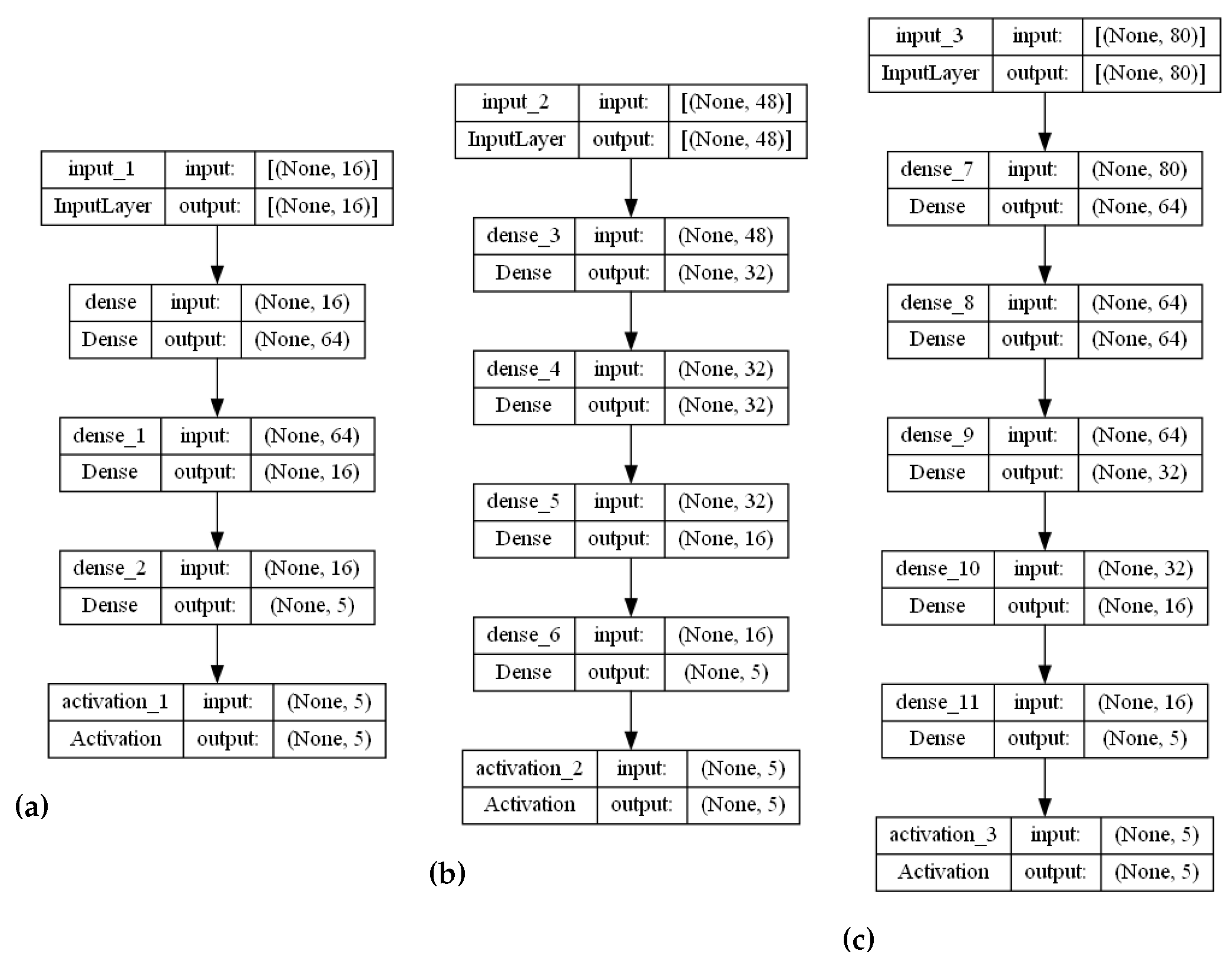
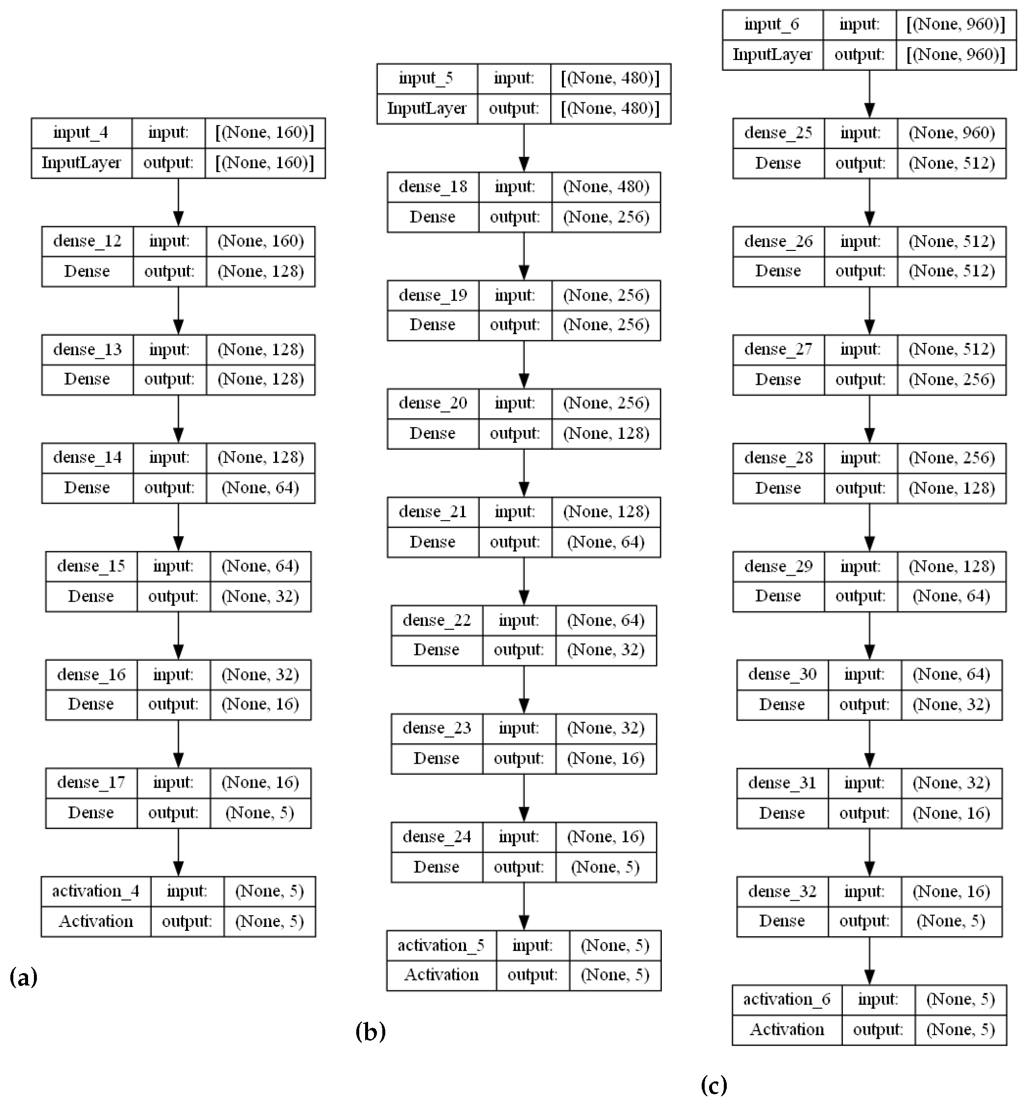
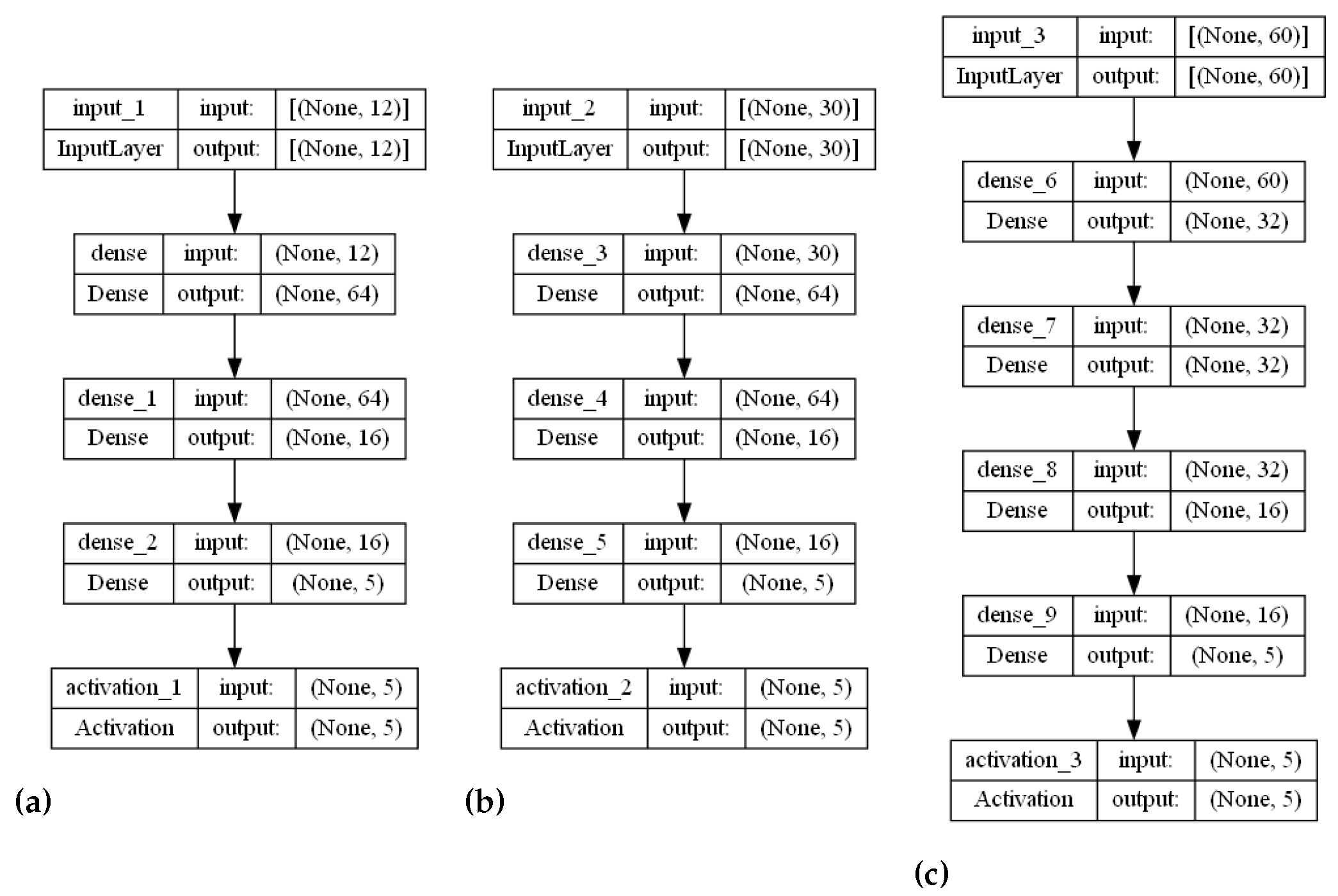
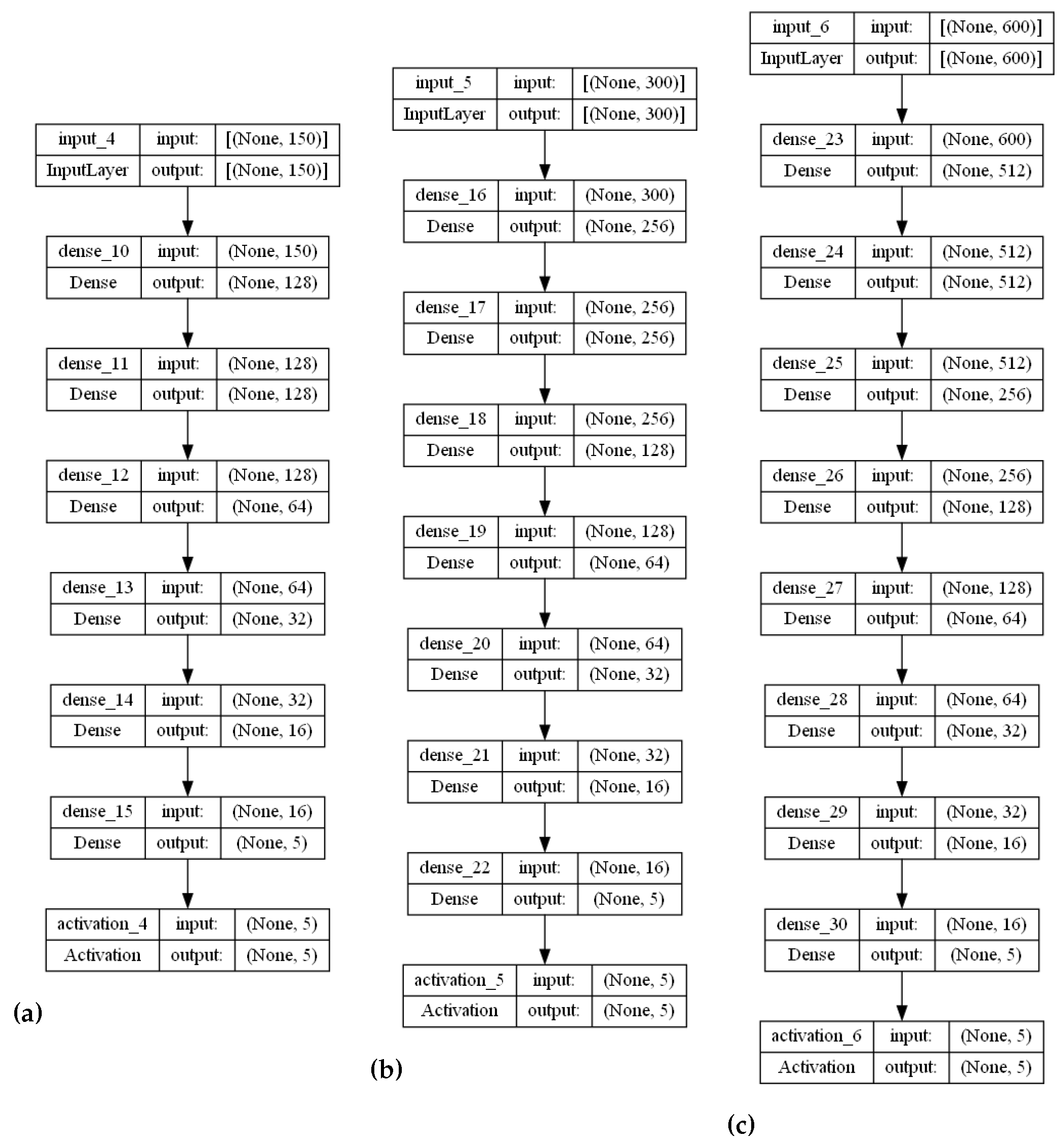
The stranded-NN model accepts different time series sensory measurements over time (m) as input. Then, according to the m value, it automatically generates fully-connected hidden layers of perceptrons. For example, let us assume that a piece of monitoring equipment has a set of $k=16$ temperature sensors, transmitting data every $dt=30$ s. In order to perform real-time malfunction detection every $T_p=3$ min, a time series of sensory measurements needs to be created to form a measurement data input batch of $m=k·\frac{Tp}{dt}=96$ measurement values. This batch of measurements needs to be annotated to an operational class. For the input value of $m=96$, the stranded-NN algorithm generates a model of three hidden layers ($L_1^{64}-L_2^{32}-L_3^{16})$, where 64, 32, 16 is the number of perceptrons for each layer. Then, the last layer is connected, collecting $L_3$ for the classification output i classes layer. For close-to-real-time detection of 10 min intervals, a batch of the total size of $m=16·20=320$ measurements data needs to be annotated (classified). For this batch input, the stranded-NN algorithm generates a model of five hidden layers $(L_1^{256}-L_2^{128}-L_3^{64}-L_4^{32}-L_2^{16})$, where 256, 128, 64, 32, 16 is the number of perceptrons per layer accordingly. In real-time cases where the number of monitoring equipment sensors is limited (for example, $k=2$ temperature sensors), small batch values (for example, $m=12$) are used. The stranded-NN algorithm cannot generate enough hidden layers for such small values. That is why a threshold value of $m=32$ was added in order for the stranded-NN algorithm to be able to generate at least a two hidden layer model ($L_1^{64}-L_2^{16}$) of 64 and 16 perceptrons per layer accordingly.

In order to eliminate degraded gradients, L1 regularization is performed over the cross entropy loss function in each hidden layer, according to Equation (3):

$${\displaystyle MLF=-\frac{1}{N}\sum _{n=1}^N\sum _{i=1}^{K}p{n}_i·lo{g}_2{y}_{ni}+\lambda \sum _{k=1}^l\left|W_k\right|,}$$

(3)

where $MLF$ is the modified loss function for the NN layer, N is the number of samples, K is the number of detection classes, $p{n}_i$ is the indicator value that the sample n belongs to class i, $y_{ni}$ is the probability that the strand associates the nth input with class i, and ${\sum }_{k=1}^l\left|W_k\right|$ is the sum of the layer absolute weight values. Parameter $\lambda$ is set to $0.005$ as derived by experimentation for all model strands. Table 1 summarizes the hyperparameters accessible for each strand and their tuned values.

Table 1. Hyperparameters tuning per strand of the stranded-NN model.

Hyperparameter	Description	Tuned Value
q	Number of hidden layers per strand	$2\le q\le 12$
$\lambda$	L1 regularization parameter	0.005
$p_{drop}$	Drop probability of dropout layers	$0.05\le p_{drop}\le 0.1$
$m_{max}$	Maximum number of input measurements per batch	4096
${\lambda }_t$	Learning rate parameter	${10}^{-4}\le {\lambda }_t\le 0.01$
${\lambda }_d$	Learning rate decrease coefficient	0.2
$n_s$	Number of stranded model strands	$2\le n_s\ge 32$
$C_{max}$	Maximum number of outputs—detection classes	16
$Epochs$	Number of train epochs	20–80
$Batc{h}_{size}$	Batch size of train data	32, 64, 128, 256, 512

To eliminate over-fitting issues, especially for datasets with a limited number of batch data, dropout layers can be introduced among layers as follows:

• For even numbers of q, a dropout layer can be inserted after every even layer depth;
• For odd numbers of q, a dropout layer can be inserted after every odd layer depth after the first hidden layer.

The use of dropout layers for the model is not obligatory. Nevertheless, in cases of over-fitting, dropouts can be set uniformly across all strands of the stranded-NN network if requested. The drop probability of each layer can be determined via fine-tuning experimentation to minimize catastrophic drops. As a guideline from the authors’ experimentation, the drop probability may be a randomly set value per layer between 0.05 and 0.1. For values above 0.1, significant losses and accuracy degradation were observed. The stranded-NN model can be used with or without including dropout layers. For big data input cases, the use of dropouts is not recommended.

To limit the number of constructed layers, as the value of batch measurements m increases, a layer limit was set, such as $q\le 12$. The value of $m=4096$ measurements per input batch was set as a measurements’ threshold value to cover even the cases of periodic checks. Nevertheless, it is considered a hyper-parameter by the stranded model. It can be altered if more frequent sensory probing is performed (less than 10 s) or a big set of sensory observations is collected per machinery asset (more than 128 observations per real-time interval).

During the per-strand training process of the stranded-NN model, the Adam solver was used with the categorical cross entropy as a loss function. The learning rate parameter ${\lambda }_t$, which defines the per-strand weight adjustments over the loss function, was initially set to $0.01$ for all model strands. If, while training, the strand validation loss decreases between epochs, then the ${\lambda }_t$ is decreased by a learning rate decrease factor ${\lambda }_d=0.2$. This is performed until the ${\lambda }_t$ parameter reaches the value of ${10}^{-4}$. Below, further ${\lambda }_t$ decreases, triggered by validation loss decays, do not contribute significantly to the NN weights.

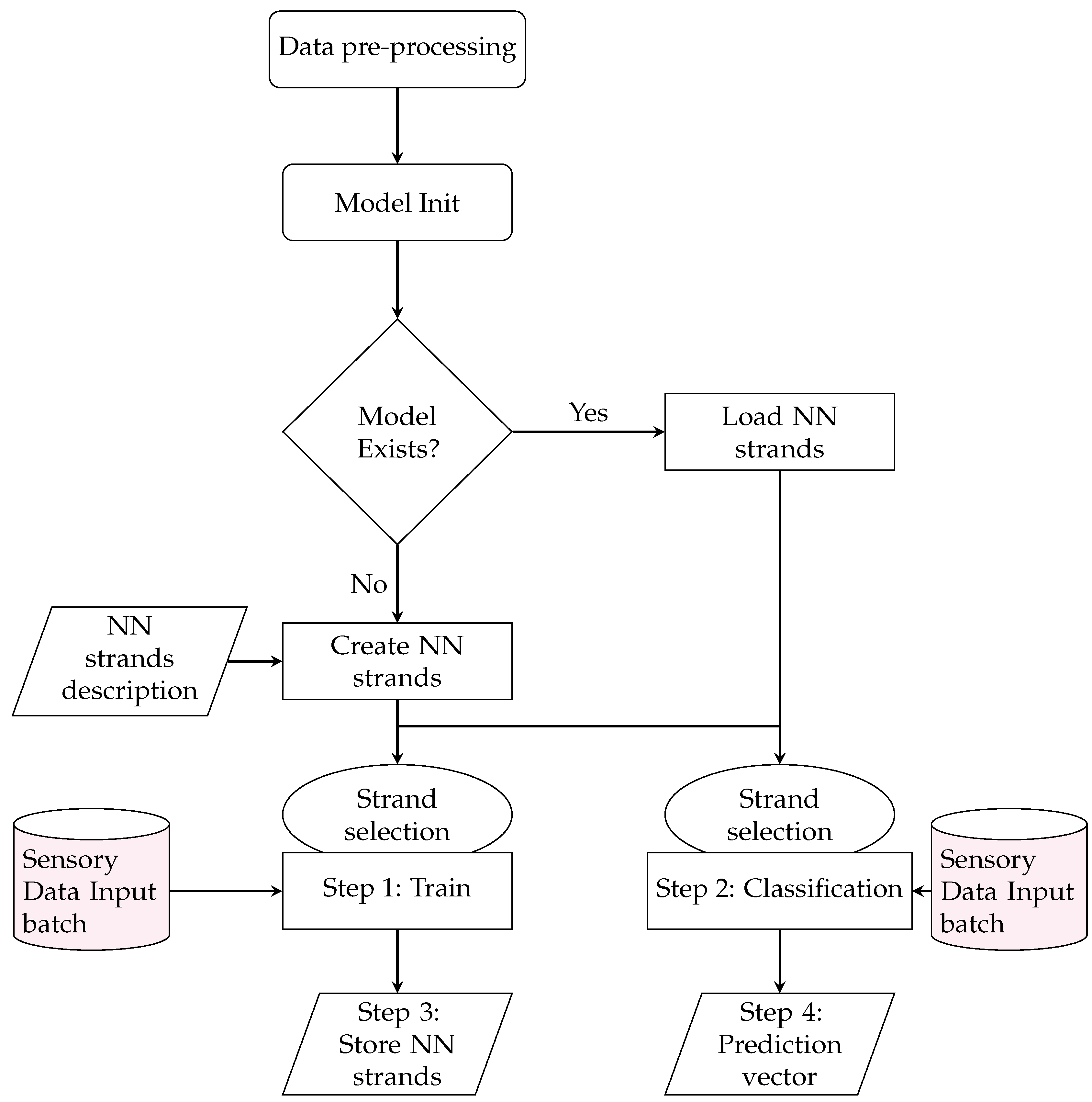
The stranded-NN model is a collection of NN-strands, which can be used for either training or classification based on the input measurements batch size. Figure 1 illustrates the stranded model training and prediction process flow. At the initialization of the NN strands, the description configuration file is parsed, and the initial NN strands are generated and attached to the model. Upon first strand creation, the model is stored with initial weights using a separate model file per NN strand using the HDF5 data format. Upon successful model storage, the model select command can select a specific NN strand of specified data input and model depth. The stranded-NN algorithmic process includes the following steps for both models training and predictions:

Figure 1. Strand-NN model training and prediction process.

Data Preprocessing: The data pre-processing step includes arranging the data input streams to 1D $(n,1)$ arrays, where n is the corresponding model strand input (stranded model input batch size). The data pre-processing also includes transforming the annotated outputs to binary 1D vectors with sizes equal to the stranded model classes. After the pre-processing, the stranded model initialization occurs, which involves either the creation of the stranded model and its corresponding strands or the stranded model load (load of strands’ weights).

Step 1—Training: In this step, the selected strand is trained using the appropriate sensory batch as data input. The model uses a configurable batch size and epoch values per selected strand for the training process. The train data split ratios to validation, and testing sets are also configurable. The default value of $0.1$ (10% of the training dataset) was used for the validation set. The default value of $0.2$ (20% of the training dataset) was used for strand evaluation. The training data set input batches were also shuffled prior to training. Since the sensory measures were in chronological order for all input batches and were classified as a batch, the shuffling process did not affect the order of the time intervals (batch size) that we wanted to have a classification outcome.

Any number can be used between 20–80 epochs for the training process epochs. However, the authors selected the size of 40 epochs, 10 epochs above the learning rate reduction initialization to be considered during the training process (fine tuning of trainable parameters). Regarding the training and evaluation batch input sizes, an arbitrary number between $16-512$ can be selected. No significant accuracy or loss changes were detected from the batch size variations in the reported range, as reported by our experimentation.

Step 2—Classification: In this step, the classification-class selection response of the selected strand is calculated using appropriate sensory batched data as input.

Step 3—Store NN strands: Upon training, the new model strand weights are stored in the new model file in the NN-model strand directory. Additionally, the strand model evaluation results regarding loss and accuracy are stored in the stranded-NN model’s output results file.

Step 4—Prediction vector output: If requested, the predictions of the output layer can be separately stored before the appliance of the soft-max activation function. This output vector is called a regression or predictions vector. It can be used in order to have the unregulated output of the strand as an input to other algorithmic output correlation, similarity, or regression processes.

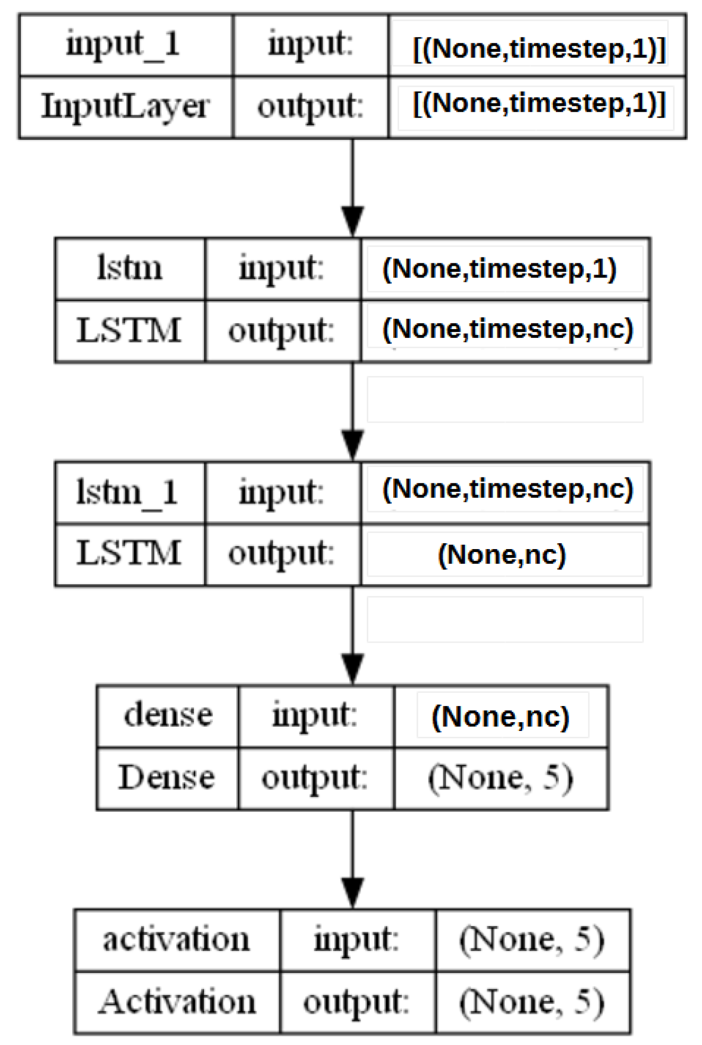
According to Table A1, the maximum number of trainable strand parameters is 15.3 M (4096 inputs per time interval), and the maximum size for this strand is 61.5 MB. Since multiple strands can co-exist in a stranded model, the total stranded model size varies as a cumulative sum of strands’ train parameters and sizes. The following section puts to the test the stranded-NN using two distinct evaluation IIoT scenarios. The model results are then compared to existing MLP [19,20,45] and LSTM implementations [27,37,46].

4. Experimental Scenarios

To evaluate their proposed stranded-NN model, the authors experimented with two different datasets:

Stranded-NN implementation using compressor temperature data. A temperature dataset, provided by two sets of the 1402 compressor of the Hellenic petroleum company. Each set includes a series of four temperature sensors (a total of eight temperature measurements/minute).

Stranded-NN implementation using pumps axial acceleration data. The measurements of normal and imbalanced pump cases are provided by the Mafaulda dataset [42]. The sensors used include three industrial accelerometers in the radial, axial, and tangential directions and a triaxial accelerometer (a total of six measurements per second).

All sensors were coupled to the pump’s axis. The pump was 250 W (0.33 Hp) with a 16 mm axis diameter and 520 mm of axis length, and a coupling bearings distance of 390 mm. A total of six measurements were provided by the accelerometers every 5 s. In addition, the measurement data of fixed rotational pump speeds of 737 rpm were used to simplify the problem further. Furthermore, it is hard to distinguish pump vibrations using vibration sensors at the pump’s mounting plate at such low rotation speeds. The acceleration data unit of measure was m/s${}^2$.

For Scenario I, of compressor temperatures, a stranded-NN model has been constructed with strands of data inputs $n=16, 48, 80$ and no dropout layers for real-time classification (see Figure A1 at Appendix A.1), signifying a batch of measurements of 1 min for $n=16$, 3 min for $n=48$ and 5 min for $n=80$. For close-to-real-time measurement, strands of data inputs $n=160, 480, 960$ were used for 10, 30, and 60 min accordingly (see Figure A2 at Appendix A.2).

For Scenario II of pump acceleration measurements, a stranded-NN model was constructed with strands of data inputs $n=12, 30, 60$ and no dropout layers for real-time classification (see Figure A3 at Appendix B.1) and strands for data inputs $n=150, 300, 600$ for close-to-real-time classification (see Figure A4 at Appendix B.2).

For both scenarios, the annotated data use five classes, indicating maintenance emergencies or critical machinery operations. The first class indicates normal behavior. The second class indicates close-to-normal machinery behavior that needs future maintenance attendance. The third class indicates stressed behavior that requires persistent monitoring and/or immediate maintenance. The fourth class indicates critical alert behavior that requires response actions, while the fifth class represents catastrophic cases that will stress the equipment beyond its intended use, as defined by machine specifications.

4.1. Scenario I: Training and Evaluating Compressor Temperatures

Given a big dataset with millions of paired (temperature, alert) values produced by a set of sensors (Figure 2), it is mandatory to annotate each temperature $T_i$ to one of the five characteristic classes according to Table 2. Once the dataset was annotated, then it is split into a training set ($80\%$) and a testing set ($20\%$).

Figure 2. Temperature sensors grouped by alert thresholds. Sets 3 and 7 contain 8 sensors each, which are related to alert = 60 °C.

Table 2. Annotation process of a given set of temperature values $T_i$, correlated to a given $alert$ threshold (in the temperature case $alert=$ 60 °C).

Class	State	Range of Temperature ${\mathit{T}}_{\mathit{i}}$
0	Normal	$0\le T_i<0.25\ast alert$
1	Low-Risk	$0.25\ast alert\le T_i<0.5\ast alert$
2	Caution	$0.5\ast alert\le T_i<0.75\ast alert$
3	Critical	$0.75\ast alert\le T_i<alert$
4	Danger	$alert\le T_i$

The constructed annotated dataset contains 7,439,584 temperature samples, and the number of samples per class is described in Table 3. To this point, it should be mentioned that, unluckily for the majority of classes $\{0,1,2,3\}$, data are collected, and class 4, related to measurements above the alert threshold, lacks real data. The experimental results follow.

Table 3. Number of temperature samples per class.

Class	Number of Samples
0	50,248
1	3,077,880
2	4,291,731
3	19,725
4	0

4.2. Scenario I: Experimental Results

In order to compare the performance of the proposed stranded-NN model against a real-time model and a close-to-real-time model, the MLP Classifier and the LSTM model were selected, respectively. In the case of the MLP classifier, several hidden layers along with a set of number of units per hidden layer were tested and the most representative models are presented in Table 4. Additionally, the LBFGS optimizer was used with a parameter $alpha={10}^{-5}$. The maximum number of iterations was set equal to 10,000. From the experimental results, it is obvious that the MLP classifier presents a maximum accuracy of $0.753$ at its deep MLP (100-layers, 20-perceptrons) representative model, with a significant loss value of $4.53$. It is also worth mentioning that an MLP (10-layers, 4-perceptrons) model is outperformed in terms of 3.9% accuracy by the MLP (100, 20) model.

Table 4. Evaluation of different in size trained MLP models on temperature data for the real-time case.

Real-Time
No of Hidden Layers	No of Perceptrons/Layer	Loss	Accuracy
2	7	$5.12$	$0.678$
3	7	$4.94$	$0.724$
5	7	$5.34$	$0.626$
10	4	$4.96$	$0.723$
25	20	$4.82$	$0.734$
50	20	$4.67$	$0.741$
100	20	$\mathbf{4.53}$	$\mathbf{0.753}$

The architecture of the LSTM model consists of two LSTM layers with an equal number of units ($nc$), while it produces an output layer for the class prediction, as is depicted in Figure A5. Table A2 in Appendix D highlights the number of units per LSTM layer, along with the number of trainable parameters and the corresponding model sizes in KB. From Table A2, the 16–16 and 60–60 LSTM models were selected as representatives of real-time and close-to-real-time cases, based on the number of trainable parameters with respect to the stranded-NN model (see Table A1 in the Appendix D). Table 5 presents the results in terms of accuracy and loss of the most representative LSTM variations depending on the underlying memory size ($nc\times 2$) and the Timestep resulting in their corresponding losses and accuracies.

Table 5. Evaluation of different memory cell sizes ($nc\times 2$) for the LSTM model on temperature data for the real-time and close-to-real-time cases, where $nc$ is the number of units per LSTM layer.

		Real-Time		Close-to-Real-Time
Memory Size (nc × 2)	Timestep	Loss	Accuracy	Loss	Accuracy
$16\times 2$	200	$0.116$	$0.952$	-	-
$60\times 2$	1000	-	-	$0.124$	$0.940$

Table 6 presents an extensive search for the best parametrization of the proposed stranded-NN model, with and without dropout layers. Lastly, Table 7 summarizes the performance of the three compared models, resulting into a proof that the proposed model performs fairly close to the LSTM performance, with a slight superiority of the LSTM model in the close-to-real-time cases, while both models outperform the MLP. Taking into consideration the fact that the collected temperature measurements lack a high jitter value and are of uniform variation, it is unquestionable that a more complicated dataset must be chosen to further investigate the performance of stranded-NN and LSTM; thus, their performance on the MaFaulda vibration dataset is presented in the next experimental section.

Table 6. Evaluation of different input sizes for the stranded-NN model on temperature data for the real-time and close-to-real-time cases and with dropout layers (in parentheses).

	Real-Time		Close-to-Real-Time
Input Size	Loss	Accuracy	Loss	Accuracy
16	$0.295\left(\mathbf{0.353}\right)$	$0.929\left(\mathbf{0.887}\right)$	-	-
48	$0.174\left(0.566\right)$	$0.951\left(0.807\right)$	-	-
80	$\mathbf{0.128}\left(0.377\right)$	$\mathbf{0.954}\left(0.848\right)$	-	-
160	-	-	$\mathbf{0.311}\left(\mathbf{0.365}\right)$	$\mathbf{0.892}\left(\mathbf{0.862}\right)$
480	-	-	$0.671\left(0.771\right)$	$0.866\left(0.826\right)$
960	-	-	$1.81\left(3.299\right)$	$0.386\left(0.583\right)$

Table 7. Evaluation of the trained stranded-NN, LSTM, and MLP models on temperature data for both real-time and close-to-real-time cases. In the case of the MLP and stranded-NN models, the best performances are selected, according to Table 4 and Table 6, respectively.

	Real-Time		Close-to-Real-Time
Model	Loss	Accuracy	Loss	Accuracy
Stranded-NN	$0.128$	$\mathbf{0.954}$	$0.311$	$0.892$
LSTM	$\mathbf{0.116}$	$0.952$	$\mathbf{0.124}$	$\mathbf{0.940}$
MLP	$4.53$	$0.753$	-	-

4.3. Scenario II: Training and Evaluating Industrial Pump Vibrations

In the case of vibration measurements, the Mafaulda dataset was used. The constructed annotated dataset for the pump’s rotation contains 1,500,000 acceleration samples (six measurements per sample). The applied load on the pump axis was modeled by appropriate Relative Centrifugal Force (RFC), applied on the pump axis of 6 g for class 1, 10 g for class 2, 20 g for class 3, and 30–35 g for class 4. Class 0 indicates normal operation (no RFC appliance). The relation between RFC and rotation speed (RPMs) is given by Equation (4).

$$V_r=\sqrt{\frac{F_g}{1.118·r}·{10}^5},$$

(4)

where $V_r$ is the axis rotation speed in revolutions per minute (RPMs), $F_g$ is the RFC force expressed in g, and r is the rotational radius. Once the dataset is annotated, it is split into a training set ($80\%$) and a testing set ($20\%$). Table 8 presents the number of samples per class, each with six accelerations measurements, two for each axis of reference $X,Y,Z$ accordingly.

Table 8. Number of vibration samples per class.

Class	Description	Number of Samples
0	Normal behavior	250,000
1	6 g RFC	250,000
2	10 g RFC	250,000
3	20 g RFC	250,000
4	30, 35 g RFC	500,000

4.4. Scenario II: Experimental Results

In this section, cross-comparison between the proposed stranded-NN model and the LSTM model are described. Since MLP performed significantly worse than both the other two models in the previous experiment, it is not taken into consideration. Table 9 and Table 10 present the performances of two representative parametrizations of the LSTM model and three of the proposed models, respectively, for real-time and close-to-real-time cases.

Table 9. Evaluation of different memory sizes ($nc\times 2$) for the LSTM model on MaFaulDa vibration data [42] for the real-time and close-to-real-time cases, where $nc$ is the number of units per LSTM layer.

		Real-Time		Close-to-Real-Time
Memory Size (nc × 2)	Timestep	Loss	Accuracy	Loss	Accuracy
$12\times 2$	200	$0.419$	$0.790$	-	-
$16\times 2$	200	$\mathbf{0.306}$	$\mathbf{0.839}$	-	-
$60\times 2$	1000	-	-	$1.593$	$0.280$
$150\times 2$	1000	-	-	$\mathbf{1.187}$	$\mathbf{0.397}$

Table 10. Evaluation of different input sizes for the stranded-NN model on vibration data for the real-time and close-to-real-time cases.

	Real-Time		Close-to-Real-Time
Input Size	Loss	Accuracy	Loss	Accuracy
12	$0.425$	$0.792$	-	-
30	$0.396$	$0.823$	-	-
60	$\mathbf{0.310}$	$\mathbf{0.859}$	-	-
150	-	-	$\mathbf{0.858}$	$\mathbf{0.652}$
300	-	-	$0.917$	$0.640$
600	-	-	$0.898$	$0.647$

Table 11 summarizes the obtained results, signifying the absolute superiority of the proposed stranded-NN model against the corresponding ones of the LSTM model in both real-time and close-to-real-time cases. As shown in the summary Table for the real-time case (see Table 11), of stranded-NN with batch size 60, the stranded-NN slightly outperforms the LSTM (16 × 2) real-time model by 2.32% in terms of accuracy, even if LSTM maintains a slightly smaller loss. For close-to-real-time cases, the representative stranded-NN model with a batch input size of 150 values significantly outperforms the LSTM (150 × 2) model by 39% in terms of accuracy and 27.7% in terms of loss. It also outperforms the corresponding close to real time LSTM (60 × 2 × 1000) model in terms of size and parameters (see Table A1 and Table A2 in the Appendix D, total trainable parameters and sizes of LSTM and stranded-NN models), by 57% in terms of accuracy and 46% in terms of loss.

Table 11. Summary evaluation table of the trained stranded-NN and LSTM models on vibration data for real-time and close-to-real-time cases.

	Real-Time		Close-to-Real-Time
Model	Loss	Accuracy	Loss	Accuracy
Stranded-NN	$0.310$	$\mathbf{0.859}$	$\mathbf{0.858}$	$\mathbf{0.652}$
LSTM	0.306	0.839	1.187	0.397

5. Discussion of the Results

The proposed stranded-NN model can carry several strands and selectively train and predict using one of its strands, as mentioned. The strand n parameter is mainly determined by the number of time-sequential measurements used by the strand as data inputs, mentioned as input batch size. The n value also defines the number of hidden layers and parameters created for each strand. Based on this n value, the authors can differentiate strands for real-time detection (small n values), close-to-real-time detection (medium n values), and periodic maintenance detection (high n values). For long strands, the stranded-NN model may face gradient elimination issues. A series of batch normalization layers need to be introduced to deal with such issues. The authors also identified the maximum number of layers for their stranded model where such a normalization process requires l = 10–12 layers.

The experimental results have shown that the stranded-NN model significantly outperforms the best MLP (100, 20) model of 100 layers and 20 perceptrons/layer. That is at least double the number of layers and parameters than the real-time NN strands. Moreover, for real-time cases, stranded-NN outperforms the MLP (100, 20) model by 15–21% in terms of accuracy and by at least 10–14% for close-to-real-time events. That is, when building very deep MLP NNs, the vanishing gradients problem starts to appear. Furthermore, the use of random dropout layers at the stranded-NN model reduces, as expected, the model’s accuracy by 2–8%. However, it still maintains a better performance footprint than its MLP counterpart. Dropout layers in the stranded-NN models are recommended only in cases of over-fitting or due to limited training datasets. LSTM models with a small number of cells ($2,4,6$) were not taken into account for real-time cases. Only LSTMs with 12–16 cells were considered real-time models, because they maintain the same number of trainable parameters with their corresponding real-time strands of the stranded-NN model (see Appendix D, Table A1 and Table A2). Taking the previous into account, for the close-to-real-time cases, the LSTM models with 42–80 cells were considered. Therefore, post-processing periodic maintenance processes can utilize LSTMs of 80 cells and above.

The experimental results of the stranded-NN model and LSTM model for real-time results have shown that the stranded-NN models slightly outperform the corresponding LSTM models by 2–3%. Nevertheless, for close-to-real-time cases, the corresponding LSTM models fail significantly, by at least 39% in terms of accuracy (39–57%) and 27% in terms of loss (27–46%). The use of high periodic intervals in the LSTM models, especially for sensory measurements that vary over time, causes LSTM models to fail significantly as predictors or classifiers. Even if more cells are used, the outcome results are still disappointing. This is, of course, not the case for small time interval annotated measurements, where LSTM models perform well. Furthermore, the LSTM model requires significantly more time to train concerning stranded-NN model strands. From the authors experimentation with close-to-real-time detections, the authors also faced one case in Scenario I where the LSTM (60) model presented 4% better accuracy results than the best close-to-real-time stranded-NN (160) model. Nevertheless, this case has been considered as an over-fitting one, due to the threshold-based data annotation. Scenario II experimentation has proven that, for all cases, the LSTM presents significantly less accuracy than the close-to-real-time stranded-NN models.

The authors have also experimented by deploying their MLP LSTM and stranded-NN implementations in an Industrial Shields PLC data collector [47]. That is, an industrial automation component and concentrator device, capable of real-time online training and detection. This PLC component includes a 64bit, 1.5 GHz Broadcom BCM2711, Quad-core Cortex-A72 (ARM v8) SoC with 4 GB of RAM. Table 12 presents the training execution time results of the three algorithms using a fixed-size dataset of 7,439,584 temperature samples as input. Detection times have not been taken into account since the classification processes per sample are fast enough for all algorithms, close to $8.14\times {10}^{-4}$ s for the LSTM model, $3.19\times {10}^{-6}$ s for the MLP model, and $3.23\times {10}^{-4}$ s for the stranded-NN model.

Table 12. Execution time of training processes of the stranded-NN, LSTM models on an Industrial PLC.

Model	Train-Time/Epoch (min)	No. Train Data
MLP (100, 20)	20.5–23.1	7,439,584
Stranded-NN (80)	0.38–0.51	7,439,584
Stranded-NN (160)	0.75–1.2	7,439,584
LSTM (16)	10.95–12.41	7,439,584
LSTM (60)	18.48–20.74	7,439,584

The training performance results from Table 12 show that the LSTM (16) model requires at least 26 times more training time, and the MLP (100) 44 times more training time, than the best selected real-time stranded-NN model (80). In terms of accuracy, the stranded-NN model significantly outperforms the MLP model by 21.3% in terms of accuracy and slightly outperforms the LSTM (16) model by 2.6%. That is, the stranded-NN model can perform real-time detections adequately at the edge industrial concentrators, as well as re-train its model in significantly less time, in the presence of new annotated data streams. Regarding close-to-real-time industrial maintenance processes, the LSTM (60) model presents 5.1% better accuracy results than the best close-to-real-time stranded-NN (160) model. However, LSTM (60) training times with the industrial edge concentrator devices are 20 times longer than with the stranded-NN (160) model; that is, the training effort is significantly more.

6. Conclusions

This paper presents a new deep learning algorithm including several arbitrary NN models, called strands, as a single learning entity. Each strand accepts different batches of data input. Each stranded-NN model has been designed to require adequate layers and perceptrons, achieving similar detection accuracies commonly used by the industry deep learning models over a time series of sensory data, such as the LSTM models. The authors also classified two significant maintenance categories: industrial real-time detection events of immediate response and periodic industrial maintenance checks. The proposed stranded-NN algorithm’s detection time depth can be implemented using different NN models for real-time and close-to-real-time data intervals (called batches) for real-time detection events and elongated periodic intervals for periodic control and maintenance tasks.

For real-time and close-to-real-time classification cases, the authors compared their stranded-NN classification model accuracies to existing models, such as deep MLPs and LSTMs of various cell sizes; that is, using sensory data of compressor temperature sets and pump annotated axial acceleration measurements. From the authors’ experimentation, the stranded-NN model significantly outperformed its counterpart MLP models and performed as well as LSTM models for real-time detections (small size of annotated data input batches). The stranded-NN models significantly outperformed their LSTM counterparts for close-to-real-time events. Furthermore, it presented significantly less training time than the LSTM and MLP models if implemented as detectors in the edge industrial data concentrators, offering fast model re-training capabilities in the presence of new annotated data.

The authors set the extended evaluation of their proposed stranded-NN algorithm and representative models for periodic industrial maintenance tasks as future work; that is, experimenting with more than hourly or daily time series of sensory annotated measurements as data input. Furthermore, due to the accuracy variations of LSTM models towards close-to-real-time events, also focusing on improving the accuracies of their stranded-NN models, further testing must be performed to provide a robust solution for periodic maintenance. However, the authors do not exclude, and even set as future work, the use and experimentation of LSTM model strands for periodic events classifications and predictions. That is, LSTM models were included as strands in their proposed stranded-NN model, if they managed to outperform stranded-NN periodic models since their elongated re-training times may not significantly affect or delay the generation of predictions if implemented in industrial edge devices.

Appendix A.1. Stranded-NN Model Strands for Real-Time Classification

Figure A1. Stranded -NN model implementation for real-time temperature measurements of Industrial compressors: (a) input size of 16 measurements, $16\times T_p$ temperature inputs, (b) input size of 48 measurements, $16\times 3T_p$ temperature inputs, (c) input size of 80 measurements, $16\times 5T_p$ temperature inputs.

Appendix A.2. Stranded-NN Model Strands for Close-to-Real-Time and Periodic Classification

Figure A2. Stranded-NN model implementation for close-to-real-time and periodic temperature measurements of Industrial compressors: (a) input size of 160 measurements, $16\times 10T_p$ temperature inputs, (b) input size of 480 measurements, $16\times 30T_p$ temperature inputs, (c) input size of 960 measurements, $16\times 60T_p$ temperature inputs.

Appendix B.1. Stranded-NN Model Strands for Real-Time Classification

Figure A3. Stranded-NN model implementation for real-time axial acceleration of Industrial pumps: (a) input size of 12 measurements, $6\times 2T_p$ acceleration inputs, (b) input size of 30 measurements, $6\times 5T_p$ acceleration inputs, (c) input size of 60 measurements, $6\times 10T_p$ acceleration inputs.

Appendix B.2. Stranded-NN Model Strands for Close-to-Real-Time and Periodic Classification

Figure A4. Stranded-NN model implementation for close-to-real-time axial acceleration of Industrial pumps: (a) input size of 150 measurements, $6\times 25T_p$ acceleration inputs, (b) input size of 300 measurements, $6\times 50T_p$ acceleration inputs, (c) input size of 600 measurements/$6\times 100T_p$ acceleration inputs.

References

1. Lasi, H.; Fettke, P.; Kemper, H.G.; Feld, T.; Hoffmann, M. Industry 4.0. Bus. Inf. Syst. Eng. 2014, 6, 239–242. [Google Scholar] [CrossRef]
2. Ahmed, I.; Jeon, G.; Piccialli, F. From Artificial Intelligence to Explainable Artificial Intelligence in Industry 4.0: A Survey on What, How, and Where. IEEE Trans. Ind. Inform. 2022, 18, 5031–5042. [Google Scholar] [CrossRef]
3. Gkamas, T.; Karaiskos, V.; Kontogiannis, S. Performance Evaluation of Distributed Database Strategies Using Docker as a Service for Industrial IoT Data: Application to Industry 4.0. Information 2022, 13, 190. [Google Scholar] [CrossRef]
4. Korkmaz, M.E.; Gupta, M.; Li, Z.; Krolczyk, G.; Kuntoğlu, M.; Binali, R.; Yaşar, N.; Pimenov, D. Indirect monitoring of machining characteristics via advanced sensor systems: A critical review. Int. J. Adv. Manuf. Technol. 2022, 120, 7043–7078. [Google Scholar] [CrossRef]
5. Esteban, A.; Zafra, A.; Ventura, S. Data mining in predictive maintenance systems: A taxonomy and systematic review. WIREs Data Min. Knowl. Discov. 2022, 12, 64–71. [Google Scholar] [CrossRef]
6. Raj, A. Unlocking the True Power of Support Vector Regression 2020. Available online: https://towardsdatascience.com/unlocking-the-true-power-of-support-vector-regression-847fd123a4a0 (accessed on 22 November 2022).
7. Alsamhi, S.H.; Ma, O.; Ansari, M.S. Survey on Artificial Intelligence Based Techniques for Emerging Robotic Communication. Telecommun. Syst. 2019, 72, 483–503. [Google Scholar] [CrossRef]
8. Qiao, L.; Li, Y.; Chen, D.; Serikawa, S.; Guizani, M.; Lv, Z. A survey on 5G/6G, AI, and Robotics. Comput. Electr. Eng. 2021, 95, 307–372. [Google Scholar] [CrossRef]
9. Sinha, R.; Patil, S.; Gomes, L.; Vyatkin, V. A Survey of Static Formal Methods for Building Dependable Industrial Automation Systems. IEEE Trans. Ind. Inform. 2019, 15, 3772–3783. [Google Scholar] [CrossRef]
10. Seshia, S.A.; Sadigh, D.; Sastry, S.S. Toward verified artificial intelligence. Commun. ACM 2022, 65, 46–55. [Google Scholar] [CrossRef]
11. Krichen, M.; Mihoub, A.; Alzahrani, M.Y.; Adoni, W.Y.H.; Nahhal, T. Are Formal Methods Applicable To Machine Learning And Artificial Intelligence? In Proceedings of the 2022 2nd International Conference of Smart Systems and Emerging Technologies (SMARTTECH), Riyadh, Saudi Arabia, 22–24 May 2022; pp. 48–53. [Google Scholar] [CrossRef]
12. Huang, C.; Deep, A.; Zhou, S.; Veeramani, D. A deep learning approach for predicting critical events using event logs. Qual. Reliab. Eng. Int. 2021, 37, 2214–2234. [Google Scholar] [CrossRef]
13. Bonissone, P.; Badami, V.; Chiang, K.; Khedkar, P.; Marcelle, K.; Schutten, M. Industrial applications of fuzzy logic at General Electric. Proc. IEEE 1995, 83, 450–465. [Google Scholar] [CrossRef]
14. James, D.J.G.; Burnham, K.J. A fuzzy-logic approach to industrial control problems. Artif. Life Robot. 1997, 1, 59–63. [Google Scholar] [CrossRef]
15. Kontogiannis, S.; Kokkonis, G. Proposed Fuzzy Real-Time HaPticS Protocol Carrying Haptic Data and Multisensory Streams. Int. J. Comput. Commun. Control. 2020, 15, 1–20. [Google Scholar] [CrossRef]
16. Leukel, J.; González, J.; Riekert, M. Adoption of machine learning technology for failure prediction in industrial maintenance: A systematic review. J. Manuf. Syst. 2021, 61, 87–96. [Google Scholar] [CrossRef]
17. Al-Garni, A.Z.; Jamal, A. Artificial neural network application of modeling failure rate for Boeing 737 tires. Qual. Reliab. Eng. Int. 2011, 27, 209–219. [Google Scholar] [CrossRef]
18. Pliego Marugán, A.; Peco Chacón, A.M.; Garcà a Márquez, F.P. Reliability analysis of detecting false alarms that employ neural networks: A real case study on wind turbines. Reliab. Eng. Syst. Saf. 2019, 191, 106574. [Google Scholar] [CrossRef]
19. Lorencin, I.; Anđelić, N.; Mrzljak, V.; Car, Z. Multilayer Perceptron approach to Condition-Based Maintenance of Marine CODLAG Propulsion System Components. Pomorstvo 2019, 33, 181–190. [Google Scholar] [CrossRef]
20. Orrù, P.F.; Zoccheddu, A.; Sassu, L.; Mattia, C.; Cozza, R.; Arena, S. Machine Learning Approach Using MLP and SVM Algorithms for the Fault Prediction of a Centrifugal Pump in the Oil and Gas Industry. Sustainability 2020, 12, 4776. [Google Scholar] [CrossRef]
21. Massaro, A.; Maritati, V.; Galiano, A.; Birardi, V.; Pellicani, L. ESB platform integrating KNIME data mining tool oriented on Industry 4.0 based on artificial neural network predictive maintenance. Int. J. Artif. Intell. Appl. (IJAIA) 2018, 9, 1–17. [Google Scholar] [CrossRef]
22. Ullah, I.; Yang, F.; Khan, R.; Liu, L.; Yang, H.; Gao, B.; Sun, K. Predictive Maintenance of Power Substation Equipment by Infrared Thermography Using a Machine-Learning Approach. Energies 2017, 10, 1987. [Google Scholar] [CrossRef]
23. Laptev, N.; Yosinski, J.; Li, L.E.; Smyl, S. Time-series extreme event forecasting with neural networks at Uber. In Proceedings of the International Conference on Machine Learning, Sydney, Australia, 6–11 August 2017. [Google Scholar]
24. Werth, J. LSTM for Predictive Maintenance on Pump Sensor Data. 2021. Available online: https://towardsdatascience.com/lstm-for-predictive-maintenance-on-pump-sensor-data-b43486eb3210 (accessed on 22 November 2022).
25. Peters, K. LSTM for Predictive Maintenance of Turbofan Engines. 2020. Available online: https://towardsdatascience.com/lstm-for-predictive-maintenance-of-turbofan-engines-f8c7791353f3 (accessed on 22 November 2022).
26. Man, J.; Zhou, Q. Remaining useful life prediction for hard failures using joint model with extended hazard. Qual. Reliab. Eng. Int. 2018, 34, 748–758. [Google Scholar] [CrossRef]
27. Jiang, Y.; Dai, P.; Fang, P.; Zhong, R.Y.; Zhao, X.; Cao, X. A2-LSTM for predictive maintenance of industrial equipment based on machine learning. Comput. Ind. Eng. 2022, 172, 108560. [Google Scholar] [CrossRef]
28. Yuan, Y.; Zhou, S.; Sievenpiper, C.; Mannar, K.; Zheng, Y. Event log modeling and analysis for system failure prediction. IIE Trans. 2011, 43, 647–660. [Google Scholar] [CrossRef]
29. Gkamas, T.; Kontogiannis, S.; Karaiskos, V.; Pikridas, C.; Karolos, I.A. Proposed Cloud-assisted Machine Learning Classification Process implemented on Industrial Systems: Application to Critical Events Detection and Industrial Maintenance. In Proceedings of the 2022 5th World Symposium on Communication Engineering (WSCE), Nagoya, Japan, 16–18 September 2022; Volume 1, pp. 95–99. [Google Scholar] [CrossRef]
30. Tiny, M.L. Available online: https://www.tinyml.org/ (accessed on 22 November 2022).
31. Martins, A.; Fonseca, I.; Farinha, J.T.; Reis, J.; Cardoso, A.J.M. Maintenance Prediction through Sensing Using Hidden Markov Models—A Case Study. Appl. Sci. 2021, 11, 7685. [Google Scholar] [CrossRef]
32. Yang, Z.; Kanniainen, J.; Krogerus, T.; Emmert-Streib, F. Prognostic modeling of predictive maintenance with survival analysis for mobile work equipment. Sci. Rep. 2022, 12, 8529. [Google Scholar] [CrossRef]
33. Ren, Y. Optimizing Predictive Maintenance with Machine Learning for Reliability Improvement. ASCE-ASME J. Risk Uncert. Engrg. Sys. Part B Mech. Engrg. 2021, 7. [Google Scholar] [CrossRef]
34. Bousdekis, A.; Magoutas, B.; Apostolou, D.; Mentzas, G. Review, analysis and synthesis of prognostic-based decision support methods for condition based maintenance. J. Intell. Manuf. 2018, 29, 1303–1316. [Google Scholar] [CrossRef]
35. Aydin, O.; Guldamlasioglu, S. Using LSTM networks to predict engine condition on large scale data processing framework. In Proceedings of the 2017 4th International Conference on Electrical and Electronic Engineering (ICEEE), Ankara, Turkey, 8–10 April 2017. [Google Scholar]
36. Jardine, A.K.; Lin, D.; Banjevic, D. A review on machinery diagnostics and prognostics implementing condition-based maintenance. Mech. Syst. Signal Process. 2006, 20, 1483–1510. [Google Scholar] [CrossRef]
37. Bruneo, D.; De Vita, F. On the Use of LSTM Networks for Predictive Maintenance in Smart Industries. In Proceedings of the 2019 IEEE International Conference on Smart Computing (SMARTCOMP), Washington, DC, USA, 12–15 June 2019; Volume 1, pp. 241–248. [Google Scholar] [CrossRef]
38. Jain, A.K.; Kundu, P.; Lad, B.K. Prediction of Remaining Useful Life of an Aircraft Engine under Unknown Initial Wear. In Proceedings of the 5th International and 26th All India Manufacturing Technology, Design and Research Conference (AIMTDR 2014), New Delhi, India, 12–14 December 2014; pp. 494:1–494:5. [Google Scholar]
39. Babu, G.S.; Li, X.; Suresh, S. Meta-cognitive Regression Neural Network for function approximation: Application to Remaining Useful Life estimation. In Proceedings of the 2016 International Joint Conference on Neural Networks (IJCNN), Vancouver, BC, Canada, 24–29 July 2016; pp. 4803–4810. [Google Scholar]
40. Porotsky, S.; Bluvband, Z. Remaining useful life estimation for systems with non-trendability behaviour. In Proceedings of the 2012 IEEE Conference on Prognostics and Health Management, Beijing, China, 23–25 May 2012; pp. 1–6. [Google Scholar]
41. Heimes, F.O. Recurrent neural networks for remaining useful life estimation. In Proceedings of the 2008 International Conference on Prognostics and Health Management, Denver, CO, USA, 6–9 October 2008; pp. 1–6. [Google Scholar] [CrossRef]
42. Signals, Multimedia, and Telecommunications Laboratory. Machinery Fault Database. 2021. Available online: https://www02.smt.ufrj.br/~offshore/mfs/ (accessed on 22 September 2021).
43. Keras: The Python Deep Learning API. 2020. Available online: https://keras.io/api/ (accessed on 22 March 2020).
44. Tensorflow 2.0:A Machine Learning System for Deep Neural Networks. 2020. Available online: https://tensorflow.org (accessed on 15 October 2020).
45. Magaletti, N.; Cosoli, G.; Leogrande, A.; Massaro, A. Predictive Maintenance and Engineered Processes in Mechatronic Industry: An Italian Case Study. Int. J. Artific. Appl. 2022, 13, 37–54. [Google Scholar] [CrossRef]
46. Nardo, E.D. Distributed Implementation of an LSTM on Spark and Tensorflow. 2016. Available online: https://www.slideshare.net/emanueldinardo/distributed-implementation-of-a-lstm-on-spark-and-tensorflow-69787635 (accessed on 12 December 2022).
47. Industrial Shields Company. Raspberry PLC 21. 2021. Available online: https://www.industrialshields.com/ (accessed on 12 July 2021).
Disclaimer/Publisher’s Note: The statements, opinions and data contained in all publications are solely those of the individual author(s) and contributor(s) and not of MDPI and/or the editor(s). MDPI and/or the editor(s) disclaim responsibility for any injury to people or property resulting from any ideas, methods, instructions or products referred to in the content.
Article Metrics
Citations
Article Access Statistics
Multiple requests from the same IP address are counted as one view.