Abstract
Clipping algorithms essentially compute the intersection of the clipping object and the subject, so to go from two to three dimensions we replace the two-dimensional clipping object by the three-dimensional one (the view frustum). In three-dimensional graphics, the terminology of clipping can be used to describe many related features. Typically, “clipping” refers to operations in the plane that work with rectangular shapes, and “culling” refers to more general methods to selectively process scene model elements. The aim of this article is to survey important techniques and algorithms for line clipping in 3D, but it also includes some of the latest research performed by the authors.
1. Introduction
In two dimensions, a section of a scene that is selected for display is called a clipping window because all parts of the scene outside the selected section are “clipped” off. In general, a procedure that eliminates portions of an object that are either inside or outside a specified region is referred to as a clipping algorithm or, simply, clipping. The only part of the scene that shows up on the screen is what is inside the clipping window [1]. Usually a clipping region is a rectangle in a standard position, although we could use any shape. In three dimensions, the viewing process is more complicated than its two-dimensional analogue because of the added dimension and, moreover, the fact that display devices are mostly two-dimensional [2]. A two-dimensional clipping window, corresponding to a selected camera lens, is defined on the projection plane, and a three-dimensional clipping region, called the view volume, is established. Depending on the type of projection used, the view volume takes the form of a truncated pyramid or a rectangular parallelepiped and is also known as the (view) frustum.
In the context of vector graphics, an image or an object is composed of straight line segments, and, thus, the type of clipping considered in this article is line clipping (Figure 1 and Figure 2). As large numbers of points or line segments must be clipped for a typical scene or picture, the efficiency of clipping algorithms is very significant. In many cases the large majority of points or line segments are either completely interior or completely exterior to the clipping window or volume. Therefore, it is important to be able to quickly accept or reject a line or a point [3]. This article proposes an algorithm for line clipping against a three-dimensional clipping region. The proposed algorithm is an extension of the algorithm described in [4] to the three-dimensional space.
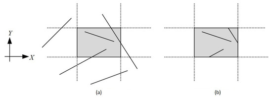
Figure 1.
(a) Before and (b) after application of line clipping in two dimensions.
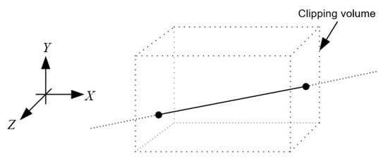
Figure 2.
A line in the three-dimensional space after clipping.
The article has the following structure. Section 2 explains the concepts of three-dimensional viewing and clipping region; Section 3 presents the classical three-dimensional line-clipping algorithms; Section 4 introduces the fundamental mathematical concepts of the line in the three-dimensional space; Section 5 describes the proposed algorithm in detail; Section 5.4 explains the steps of the algorithm in brief as well as presents a C++-based pseudocode implementation; Section 6 evaluates the proposed algorithm and its experimental results after comparison with other clipping algorithms; and, finally, Section 7 has a brief summary of all the above.
2. Three-Dimensional View Volumes and Clipping Regions
For two-dimensional graphics, viewing operations convert positions in the world coordinate plane to pixels in a screen or any other output device. Using rectangular boundaries for the clipping window, a clipping process clips a two-dimensional scene and maps it to device coordinates. Three-dimensional viewing operations are more complicated because there is an extra dimension and involves some tasks that are not present in two-dimensional viewing. To create a display of a three-dimensional world coordinate scene, one must first set up a coordinate reference for the viewing parameters (also known as the camera). This coordinate reference defines the position and orientation for a view plane (or projection plane) that corresponds to a camera film plane [1] (see Figure 3). The vertices that make up the object are then converted to the viewing reference coordinates and projected onto the view plane.
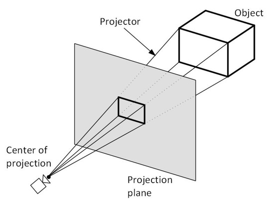
Figure 3.
Obtaining a selected view of a three-dimensional scene (camera).
Unlike a camera picture, there are different methods for projecting a scene onto the view plane. One method for getting the description of a solid object onto a view plane is to project points on the object’s surface along parallel lines. This technique, called parallel projection, is mostly used in engineering and architectural drawings to represent an object with a set of views that show accurate dimensions of the object. Another method for generating a view of a three-dimensional scene is to project points to the view plane along converging paths. This process, called perspective projection, causes objects farther from the viewing position to be displayed smaller than objects of the same size that are nearer to the viewing position. A scene that is generated using a perspective projection appears more realistic because this is the way that our eyes and a camera lens form images. Parallel lines along the viewing direction appear to converge to a distant point in the background, and objects in the background appear to be smaller than objects in the foreground (see Figure 4).
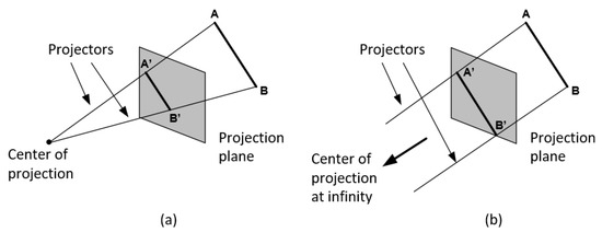
Figure 4.
(a) Line AB and its perspective projection A’B’. (b) Line AB and its parallel projection A’B’.
Most of the time, the view volume is either a rectangular parallelepiped, i.e., a box or a cuboid, or a frustum pyramid. Both of these shapes are six-sided with the following sides: left, right, top, bottom, near (hither), and far (yon); see Figure 5.
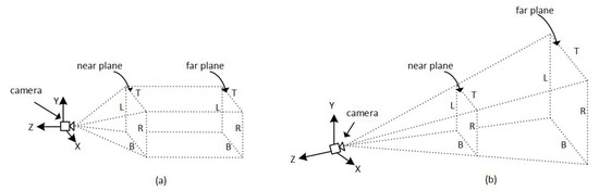
Figure 5.
Types of view volume: (a) rectangular parallelepiped, (b) truncated pyramid also known as a frustum.
After the specification of the type of view volume, various strategies can be used to implement the viewing process depending on the view volume and the 3D scene. A conceptual model could be similar to the one in Figure 6: the view volume is used as a clipping region to discard the unnecessary out-of-boundaries components of the three-dimensional scene. The remaining components are then projected onto the projection plane. Finally, the projection plane is transformed into two-dimensional device coordinates.
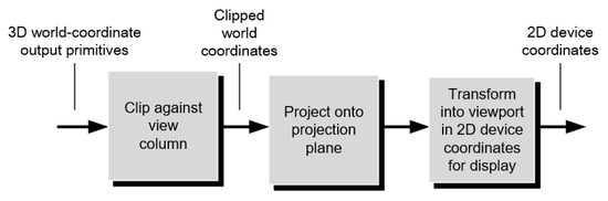
Figure 6.
Conceptual model of the three-dimensional viewing process.
Unfortunately, if the viewing is perspective and the volume is a frustum, it can be computationally expensive to check if objects exist inside the boundaries and perform clipping; see Figure 7.
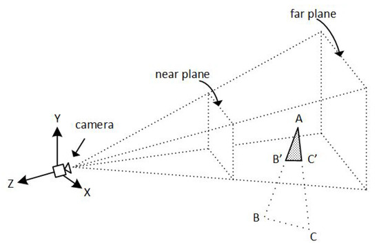
Figure 7.
A frustum-shaped clipping region is computational expensive.
In order to simplify and speed up the clipping process, an extra stage is added to the above model; see Figure 8. Before clipping and projection stages, the frustum is firstly transformed into a normalized canonical view volume. Clipping and hidden surface calculations are then applied (Figure 9).
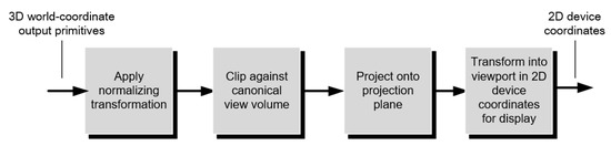
Figure 8.
Implementation of three-dimensional viewing.
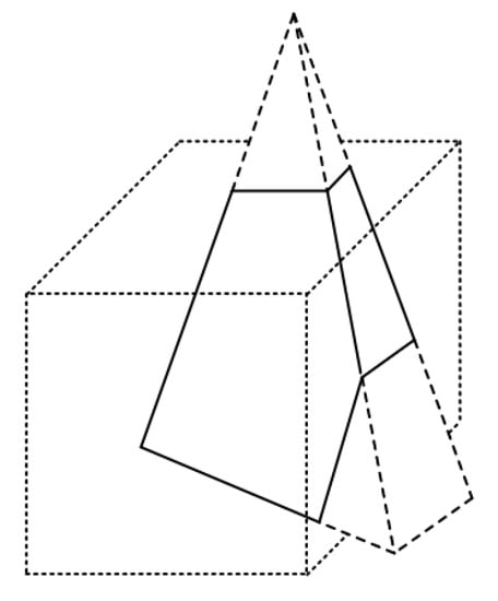
Figure 9.
Applying clipping using a normalized canonical clipping region.
3. Line-Clipping Algorithms in Three-Dimensions
There are many line-clipping algorithms in two-dimensions such as Cohen–Sutherland, Liang–Barsky [5], Cyrus–Beck [6], Nicholl–Lee–Nicholl [7], midpoint subdivision, Skala 2005 [8], S-Clip E2 [9], Kodituwakku–Wijeweere–Chamikara [10], and affine transormation clipping [11]. Unfortunately, only a few of them can clip lines in three-dimensional space. These algorithms include Cohen–Sutherland, Liang–Barsky, and Cyrus–Beck, which are considered as the classic ones for this purpose. Over the years, other algorithms for clipping a line in three-dimensional space have emerged such as simple and efficient 2D and 3D span clipping algorithms [12], Kodituwakku–Wijeweera–Chamikara 3D [13], and Kolingerova [14], but some of them do not perform clipping correctly (e.g., Kodituwakku–Wijeweera–Chamikara) while some others are hard to implement.
3.1. Three-Dimensional Cohen–Sutherland Line Clipping
The Cohen–Sutherland algorithm is considered a classic line-clipping algorithm in two dimensions. The three-dimensional analogue is very similar to its two-dimensional version but with a few modifications. For an orthogonal clipping region, the three-dimensional space is divided again into regions but this time a 6-bit region code, instead of a four-bit one, is used to classify the lines’ endpoints. These six bits are as in Figure 10.
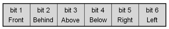
Figure 10.
Cohen–Sutherland 3D six-bit representation.
The regions are related to the space that is in front of the near plane, the space between the near and the far plane, and the space behind the far plane; see Figure 11.
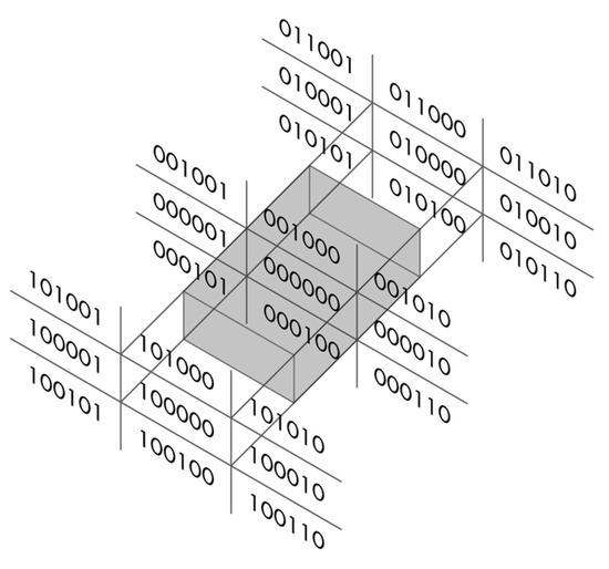
Figure 11.
Three-dimensional six-bit region codes.
The testing strategy is virtually identical to the two-dimensional case. The bit codes can be set to true (1) or false (0), depending on the test for these equations as follows:
| Bit 1: endpoint is in front of the view volume; |
| Bit 2: endpoint is behind the view volume; |
| Bit 3: endpoint is above the view volume; |
| Bit 4: endpoint is below the view volume; |
| Bit 5: endpoint is right of the view volume; |
| Bit 6: endpoint is left of the view volume. |
To clip a line, the classification of its endpoints with the appropriate region codes is required. The line is as follows:
| Visible: | if both endpoints are 000000; |
| Invisible: | if the bitwise logical AND is not 000000; |
| A clipping candidate: | if the bitwise logical AND is 000000. |
All lines with both endpoints in the [000000] region are trivially accepted. All lines whose endpoints share a common bit in any position are trivially rejected. The clipped line is derived from the parametric equation of the line in three-dimensional space using homogeneous coordinates and by using boundary coordinates whenever it is necessary.
3.2. Three-Dimensional Liang–Barsky Line Clipping
The Liang–Barsky algorithm is a line-clipping algorithm and is considered more efficient than Cohen–Sutherland [5]. It is considered to be a fast parametric line-clipping algorithm and can be applied to two dimensions as well as to three dimensions. The following concepts are used when three-dimensional clipping is applied:
- The parametric equation of the line.
- The inequalities describing each side (boundaries) of the clipping region, which are used to determine the intersections between the line and each side.
The parametric equation of a line can be given by the following equations:
where t is between 0 and 1. The point-clipping conditions in the parametric form are then written as
and the above six inequalities can be expressed as
where correspond to the left (), right (), bottom (), top (), far (), and near () boundaries, respectively. The p and q are defined as follows:
Using the following conditions, the position of the line can be determined as follows.
- When the line is parallel to a clipping boundary, the p value for that boundary is zero.
- When , as t increases the line goes from the outside to the inside (entering).
- When , the line goes from the inside to the outside (exiting).
- When and , the line is trivially invisible because it is outside the clipping region.
- When and , the line is inside the corresponding clipping region.
Parameters and can be calculated to define the part of the line that lies within the clipping region. The following points hold:
- When , is taken.
- When , is taken.
If , the line is completely outside the clipping region and it can be rejected. Otherwise, the endpoints of the clipped line are calculated from the two values of parameter t.
3.3. Three-Dimensional Cyrus–Beck Line Clipping
The Cyrus–Beck algorithm is another classic line-clipping algorithm in two-dimensional space. With simple modifications, it can also clip lines in three-dimensional space. According to the algorithm, a straight line, intersecting the interior of a convex set, can intersect the boundary of the set in, at most, two places. In the case where the convex set is closed and bounded, the straight line will intersect it in exactly two places [6].
Each side of the view volume is considered as a convex polygon in three-dimensional space and it is used as a clipping plane. This means that the algorithm examines all six planes of the view volume and performs clipping when necessary. For each clipping plane, the following steps are applied:
- The inward normal of the plane (perpendicular vector to the plane) is calculated by using three out of the four known vertices that form the plane.
- The vector of the clipping line is calculated.
- The dot product between the difference of one vertex per edge and one selected end point of the clipping line and the normal is calculated (for all edges).
- The dot product between the vector of the clipping line and the normal is calculated.
- The former dot product is divided by the latter dot product and multiplied by (this is t).
- The values of t are classified as entering or exiting (from all edges) by observing their denominators (latter dot product).
- One value of t is chosen from each group and it is put into the parametric form of a line to calculate the coordinates.
- If the entering t value is greater than the exiting t value, then the clipping line is rejected.
3.4. Three-Dimensional Kolingerova Line Clipping
In 1994, Ivana Kolingerova presented a comparative study on 3D line-clipping algorithms. Based on the Cyrus–Beck algorithm, she proposed improvements for increasing its speed. Some of these improvements were related to the way that the algorithm calculated intersection points, e.g., by using orthogonal planes, since the new methods use the fact that each line can be described as the intersection of two planes. Furthermore, unlike Cyrus–Beck, she proposed ways to end the computation earlier when finding the two intersections of the line segment against the clipping volume.
4. Mathematical Background
We consider a line L that passes through two points and in three-dimensional space (see Figure 12).
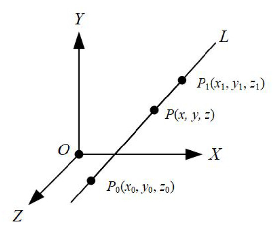
Figure 12.
Line L passing through points and .
For an arbitrary point on the line, the parametric equation of the line is
The equation of the line may also be written symmetrically as
and, if we assume that
then the equation of the line can also be written as
5. The Proposed Method
5.1. Nomenclature
Suppose that we want to clip a line inside the rectangular parallelepiped volume in Figure 13. The dimensions of the volume range from xmin to xmax for the X axis (width), from ymin to ymax for the Y axis (height), and from zmin to zmax for the Z axis (depth). The line L that is going to be clipped has endpoints P0(x0, y0, z0) and P1(x1, y1, z1) (see Figure 14).
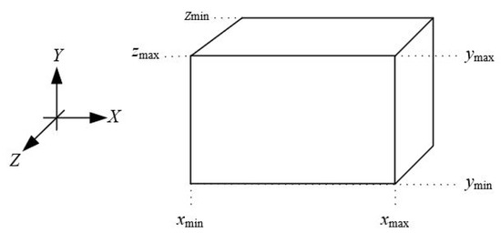
Figure 13.
Rectangular parallelepiped clipping volume.
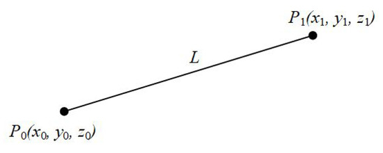
Figure 14.
Line L in three-dimensional space.
5.2. Description
The first step of the algorithm checks, if both of the endpoints are outside the clipping region and at the same time in the same region (left, right, bottom, top, near, far). If one of the following occurs, then the line is being rejected and the algorithm draws nothing; see examples of Figure 15:
| < AND < | (the line is left of the clipping region); |
| > AND > | (the line is right of the clipping region); |
| < AND < | (the line is under the clipping region); |
| > AND > | (the line is above the clipping region); |
| < AND < | (the line is behind the clipping region); |
| > AND > | (the line is in front of the clipping region). |
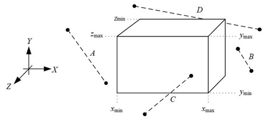
Figure 15.
Rejected lines: line A is left of the clipping region, line B is right of the clipping region, line C is in front of the clipping region, and line D is on the back of the clipping region.
In the second step, the algorithm compares the coordinates of the two endpoints of the line along with the boundaries of the clipping region. It compares the and coordinates with the and boundaries, respectively, then it compares the and coordinates with the and boundaries and, finally, it compares the and coordinates with the and boundaries. If any of these coordinates are outside the clipping boundary, then the boundary cordinates are used instead for limiting the line inside the volume and achieving clipping (see Figure 16).
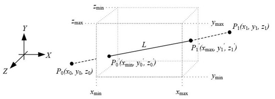
Figure 16.
Using the boundary coordinates for the endpoints of the line.
For each of the coordinates of the two endpoints, and according to Equations (2)–(5), the comparisons and the new coordinates are as follows:
- If < , then
- If , then
- If , then
- If , then
- If , then
- If , then
In the above we have that i vary from 0 to 1. In the third and final step, the algorithm draws the line between the two endpoints.
5.3. Considerations
If we look carefully at Equation (1), it seems that for certain values a division by zero may occur. Let us examine the case of the x coordinate of an endpoint. According to the second step of the algorithm, the x coordinate is being checked as to whether it is less than or greater than . If we replace and solve for y and z the new coordinates will be
Likewise, if we replace and solve for y and z the new coordinates will be as follows:
Division by zero will occur, only if . However, when and or the line is vertical to the Y axis and is totally outside the clipping region, so division by zero will never occur according to the first step’s condition. On the other hand, if then there is no need to apply clipping for the specific coordinate, so, again, division by zero will not occur in this range. Similarly, division by zero will never occur for all other coordinates.
5.4. The Steps in Brief and the Pseudocode
The steps of the algorithm are as follows:
- Check, if both endpoints of the line are outside the same side of the rectangular parallelepiped clipping region. If this is true then stop and draw nothing or else proceed to Step 2.
- Compare each coordinate of each endpoint of the line along with the boundaries of the clipping region (left, right, top, bottom, near, and far). If a coordinate is outside the clipping boundary, then use the boundary coordinate instead and calculate the other coordinates of the endpoint, respectively.
- Draw the clipped line between the two endpoints.
6. Evaluation and Experimental Results
To determine the efficiency of the proposed algorithm, we evaluate it against the Cohen–Sutherland, Liang–Barsky, Cyrus–Beck and Kolingerova algorithms. Each algorithm had to clip a large number of arbitrary lines generated in a three-dimensional space. The boundaries of this space were defined by the points (−400, −400, 400) and (400, 400, −400). The clipping region has the following dimensions: 200 pixels width, 150 pixels height, and 100 pixels depth with its centre at the centre of the screen and the start of the axes X, Y, and Z (Figure 17). The lines were randomly generated anywhere in the three-dimensional space and each algorithm drew only the visible part of the lines inside the clipping region. The time that each algorithm needed to clip the lines was recorded in every execution. The whole process was repeated ten times and, in the end, the average time was calculated.
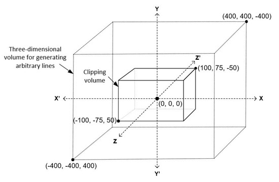
Figure 17.
The three-dimensional space used for generating arbitrary lines and setting the clipping volume.
The hardware, as well as the software, specifications for our evaluation were as follows: (a) AMD FX Quad-Core 4300@3.80 GHz CPU, (b) RAM 16 GB, (c) NVIDIA GeForce GTX-1050 GPU, (d) Windows 10 Professional operating system, (e) C++ with OpenGL/FreeGLUT under the Code::Blocks environment. Each algorithm should have clipped and drawn one million lines in every execution. The visual result was a rectangular parallelepiped volume full of clipped lines (Figure 18), whereas the evaluation results are shown in Table 1.
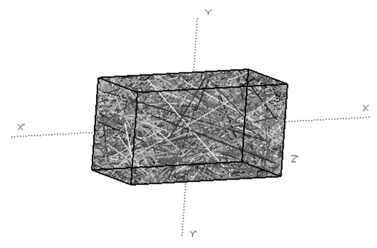
Figure 18.
One million clipped lines inside the clipping volume.

Table 1.
Execution times of each algorithm when clipping one million lines.
Using the above results, a graph for the clipping times of each algorithm was created (Figure 19).
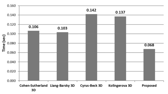
Figure 19.
Average time of each algorithm when clipping one million lines (lower is better).
By using the formula
we can evaluate the speed of the proposed algorithm in percent compared to the other algorithms. Compared to the Cohen–Sutherland algorithm, the proposed algorithm was faster by 57.16%; compared to the Liang–Barsky algorithm, our algorithm was faster by 52.73%; compared to the Cyrus–Beck algorithm, our algorithm was faster by 109.75%; and compared to the Kolingerova algorithm, our algorithm was faster by 102.66%.
The experiment was also performed for similar types of line segments, e.g., segments that were strictly inside the clipping region and did not intersect it. The results were in accordance with the above results; there were no different running times for all algorithms.
7. Summary
Line clipping is a technique that is widely used in computer graphics. The three-dimensional viewing pipeline involves many more complicated stages than its two-dimensional analogue. When a three-dimensional scene is projected onto a two-dimensional plane by using perspective projection, transforming the frustum-shaped view volume into a canonical one (rectangular parallelepiped) is considered good practice and speeds up the process since clipping against a frustum-shaped view volume is computationally expensive. In the present article, an overview of the most common, as well as of the lesser-known, algorithms for clipping a line against a rectangular region in a three-dimensional space was presented. Moreover, a simple and fast algorithm (see Algorithm 1) for clipping a line segment against a rectangular parallelepiped view volume was proposed. The algorithm is straightforward to implement in any programming language.
| Algorithm 1 The proposed algorithm |
void clip_3d_line(double x[], double y[], double z[], double xmin, double xmax, double ymin, double ymax, double zmin, double zmax) { if( !((x[0] < xmin && x[1] < xmin) || (x[0] > xmax && x[1] > xmax) || (y[0] < ymin && y[1] < ymin) || (y[0] > ymax && y[1] > ymax) || (z[0] < zmin && z[1] < zmin) || (z[0] > zmax && z[1] > zmax)) ) { double a = x[1] − x[0]; double b = y[1] − y[0]; double c = z[1] − z[0]; for(int i = 0; i <= 1; i++) { if(x[i] < xmin) { y[i] = b / a * (xmin − x[0]) + y[0]; z[i] = c / a * (xmin − x[0]) + z[0]; x[i] = xmin; } else if(x[i] > xmax) { y[i] = b / a * (xmax − x[0]) + y[0]; z[i] = c / a * (xmax − x[0]) + z[0]; x[i] = xmax; } if(y[i] < ymin) { x[i] = a / b * (ymin − y[0]) + x[0]; z[i] = c / b * (ymin − y[0]) + z[0]; y[i] = ymin; } else if(y[i] > ymax) { x[i] = a / b * (ymax − y[0]) + x[0]; z[i] = c / b * (ymax − y[0]) + z[0]; y[i] = ymax; } if(z[i] < zmin) { x[i] = a / c * (zmin − z[0]) + x[0]; y[i] = b / c * (zmin − z[0]) + y[0]; z[i] = zmin; } else if(z[i] > zmax) { x[i] = a / c * (zmax − z[0]) + x[0]; y[i] = b / c * (zmax − z[0]) + y[0]; z[i] = zmax; } } } draw_line(x[0], y[0], z[0], x[1], y[1], z[1]); } |
Author Contributions
Conceptualization, V.D.; methodology, D.M. and V.D.; software, D.M.; formal analysis, D.M.; data curation, D.M.; writing–original draft preparation, D.M.; writing–review and editing, V.D.; visualization, D.M.; supervision, V.D. All authors have read and agreed to the published version of the manuscript.
Funding
This research received no external funding.
Data Availability Statement
Not applicable.
Conflicts of Interest
The authors declare no conflict of interest.
Nomenclature
References
- Hearn, D.; Baker, M.P.; Carithers, W.R. Computer Graphics with Open GL, 4th ed.; Pearson Education Limited: Harlow, UK, 2014. [Google Scholar]
- Hughes, J.F.; van Dam, A.; McGuire, M.; Sklar, D.F.; Foley, J.D.; Feiner, S.K.; Akeley, K. Computer Graphics Principles and Practice, 3rd ed.; Addison-Wesley Professional: Boston, MA, USA, 2013. [Google Scholar]
- Rogers, D.F. Procedural Elements for Computer Graphics, 2nd ed.; McGraw-Hill, Inc.: New York City, NY, USA, 1997. [Google Scholar]
- Matthes, D.; Drakopoulos, V. Another simple but faster method for 2D line clipping. Int. J. Comput. Graph. Animat. 2019, 9, 1–15. [Google Scholar] [CrossRef]
- Liang, Y.D.; Barsky, B.A. A new concept and method for line clipping. TOG 1984, 3, 1–22. [Google Scholar] [CrossRef]
- Cyrus, M.; Beck, J. Generalized two- and three-dimensional clipping. Comput. Graph. 1978, 3, 23–28. [Google Scholar] [CrossRef]
- Nicholl, T.M.; Lee, D.; Nicholl, R.A. An efficient new algorithm for 2-D line clipping: Its development and analysis. Comput. Graph. 1987, 21, 253–262. [Google Scholar] [CrossRef]
- Skala, V. A new approach to line and line segment clipping in homogeneous coordinates. Vis. Comput. 2005, 21, 905–914. [Google Scholar] [CrossRef]
- Skala, V. S-clip E2: A new concept of clipping algorithms. In Proceedings of the SA ’12: SIGGRAPH Asia, Singapore, 28 November 2012–1 December 2012. [Google Scholar] [CrossRef]
- Kodituwakku, S.R.; Wijeweera, K.R.; Chamikara, M.A.P. An efficient algorithm for line clipping in computer graphics programming. Ceylon J. Sci. (Physical Sci.) 2013, 1, 1–7. [Google Scholar]
- Huang, W. The Line Clipping Algorithm Basing on Affine Transformation. Intell. Inf. Manag. 2010, 2, 380–385. [Google Scholar] [CrossRef]
- Duvanenko, V.J.; Gyurcsik, R.S.; Robbins, W.E. Simple and Efficient 2D and 3D Span Clipping Algorithms. Comput. Graph. 1993, 17, 37–54. [Google Scholar] [CrossRef]
- Kodituwakku, S.R.; Wijeweera, K.R.; Chamikara, M.A.P. An efficient line clipping algorithm for 3D space. Int. J. Adv. Res. Comput. Sci. Softw. Eng. 2012, 2, 96–101. [Google Scholar]
- Kolingerova, I. 3D-line Clipping Algorithms—A Comparative Study. Vis. Comput. 1994, 11, 96–104. [Google Scholar] [CrossRef]
Disclaimer/Publisher’s Note: The statements, opinions and data contained in all publications are solely those of the individual author(s) and contributor(s) and not of MDPI and/or the editor(s). MDPI and/or the editor(s) disclaim responsibility for any injury to people or property resulting from any ideas, methods, instructions or products referred to in the content. |
© 2023 by the authors. Licensee MDPI, Basel, Switzerland. This article is an open access article distributed under the terms and conditions of the Creative Commons Attribution (CC BY) license (https://creativecommons.org/licenses/by/4.0/).