Feasibility of Low Latency, Single-Sample Delay Resampling: A New Kriging Based Method

Abstract

Wireless sensor systems often fail to provide measurements with uniform time spacing. Measurements can be delayed or even miss completely. Resampling to uniform intervals is necessary to satisfy the requirements of subsequent signal processing. Common resampling algorithms, based on symmetric finite impulse response (FIR) filters, entail a group delay of 10 s of samples, which is not acceptable regarding the typical interval of wireless sensors of seconds or minutes. The purpose of this paper is to verify the feasibility of single-delay resampling, i.e., the algorithm resamples the data without waiting for future samples. A new method to parametrize Kriging interpolation is presented and compared with two variants of Lagrange interpolation in detailed simulations for the resulting prediction error. Kriging provided the most accurate resampling in the group-delay scenario. The single-delay scenario required almost double the OSR to achieve the same signal-to-noise ratio (SNR). An OSR between 1.8 and 3.1 was necessary for single-delay resampling, depending on the required SNR and signal distortions in terms of jitter, missing samples, and noise. Kriging was the least noise-sensitive method. Especially for signals with missing samples, Kriging provided the best accuracy. The simulations showed that single-delay resampling is feasible, but at the expense of higher OSR and limited SNR.

1. Problem and Motivation

The data collected from single or multiple wireless sensors provide the input for subsequent signal-processing algorithms. While signal processing mainly requires synchronized, uniform, and equidistant sampling, the transmission of wireless sensors deviates from these requirements due to issues such as lost samples during transmission, clock frequency and offset deviations between sensor nodes, random time lags after a hardware failure or reset, or the sensor sampling rate does not meet the required signal-processing sampling rate. Unpredictable delays caused by the sensor network, e.g., by waiting for a free channel, can be compensated by marking measurements with a time stamp directly on the sensor node instead of using the arrival time at the signal-processing unit. To solve remaining issues, it is necessary to resample the data using interpolation or reconstruction techniques.

1.1. The Problem of Group Delay

Two components contribute to the total delay or latency of the reconstruction algorithm: the computation time or processing delay to handle one sensor measurement and the filter’s group delay. Most recently published solutions (Section 2) are primarily designed for high frequency applications by using techniques such as Farrow filters [1] and finite impulse response (FIR) filters. The filter can be adapted to changing sampling rates and patterns [2].

In high frequency applications, the priority is to ensure that the processing delay is shorter than the sampling interval, and the filter group delay is less important. FIR filters, which have a constant group delay of half the filter order, are commonly used. For example, the group delay of audio resampling using a FIR filter with an order 90 is still under 1 ms.

Resampling data from wireless sensors requires a different design focus. Data typically come in intervals of seconds or even minutes, and group delays of tens of samples are not acceptable. If the wireless sensor system is part of a control application, new samples must be iteratively processed within a guaranteed response time and be converted to the resampled signal with low latency. Such low-latency processing is the basis for a real-time control system. However, other challenges, such as implementation on a real-time operating system, are not addressed in this paper.

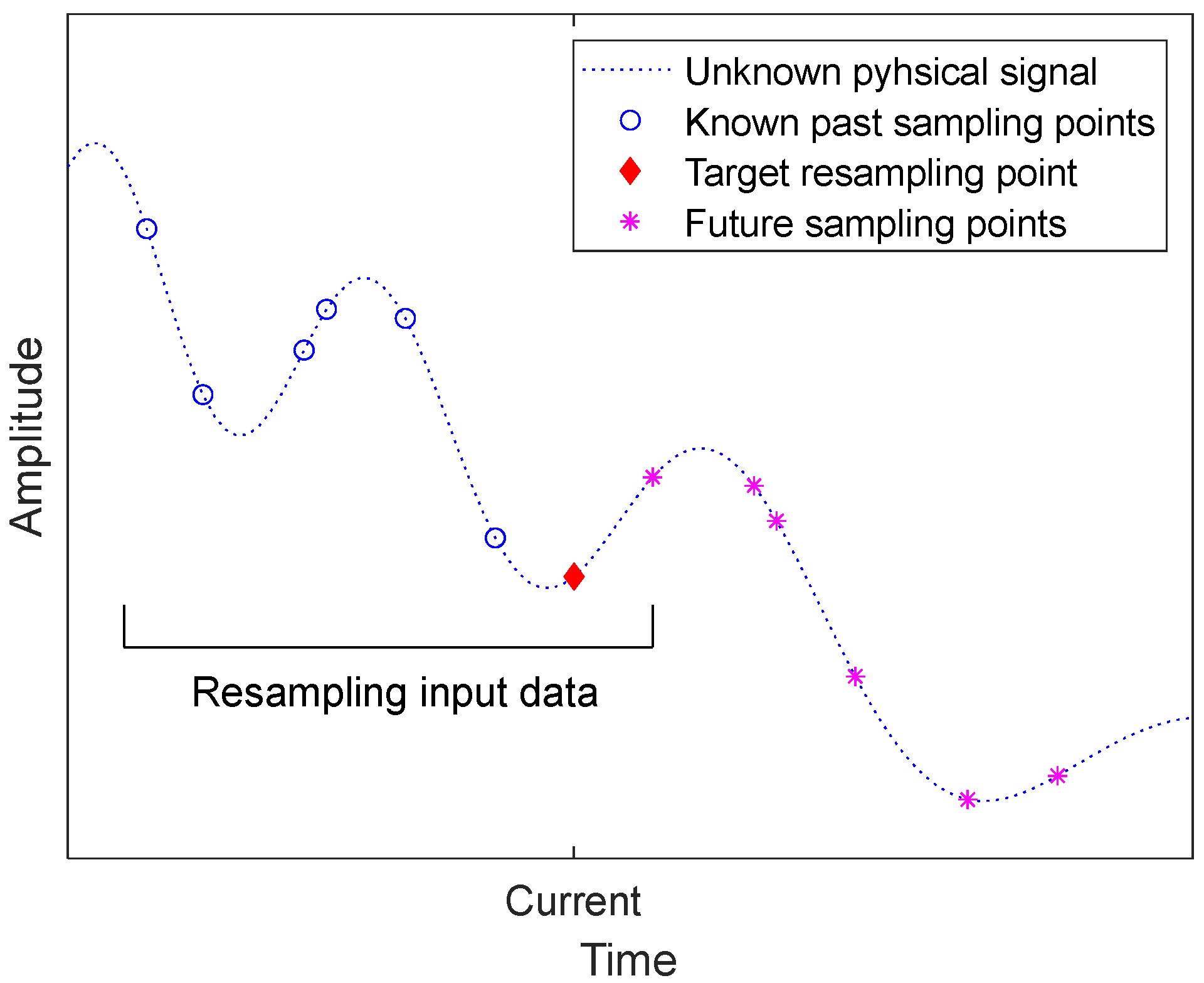
From the perspective of a target time point for calculating the resampled signal, one or multiple future sensor measurements must be known for signal interpolation (Figure 1). However, zero-delay resampling can only be applied to low-frequency signals, extrapolation beyond known past samples leads to stability problems.

Most existing approaches from the literature provide suitable solutions for the group-delay scenario. In this case, the algorithm is allowed to wait for the required number of future samples, as determined by the half FIR filter order or the half window width of the algorithm. The output is then delayed by the same number of samples. In an extended scenario, offline reconstruction of a signal is possible without any restrictions on processing delays.

The focus of this paper is on a different scenario, called the single-delay scenario, in which the resampling algorithm is only allowed to use one future sample. This means that as soon as a new sample arrives, the gap between the current and the previous sample should be reconstructed and appended to the resampled signal. Any changes in the input should be immediately reflected in the output.

This paper tests the feasibility and minimum required oversampling rate (OSR) for single-sample delay reconstruction. Furthermore, it introduces a new method based on Kriging interpolation. Either the resampling algorithm can be implemented as an event processor to update the resampled signal after the arrival of each sensor measurement, or it can be triggered by subsequent signal processing, when the signal processing is ready to receive the next input sample.

1.2. New Contribution

The present study’s new contributions are as follows: Firstly, the effect of switching from a group-delay to a single-delay scenario in terms of reconstruction accuracy is hardly evaluated in the existing literature. A detailed comparison of the error and the achievable OSR are presented in Section 4.

Secondly, a new resampling filter based on Kriging interpolation is introduced. Standard Kriging applications take statistical properties from the input signal using the variogram model for setting the Kriging parameters. Instead, we have tuned the variogram parameters to achieve a frequency response close to the desired brick-wall characteristics (Section 3.1). Accurate resampling was achieved with constant variogram parameters for a wide range of input signals. Furthermore, Kriging interpolation has the advantage of inherently scaling to non-uniform inputs without any changes in the algorithm. The new method provides low-latency resampling of uniform and non-uniform signals with a single-sample delay. Kriging required an OSR of 1.34 to achieve a signal-to-noise ratio (SNR) of 60 dB to reconstruct a jitter test signal in the group-delay scenario. The single-delay scenario was more challenging and required almost double the OSR.

Thirdly, an extended Lagrange approach, which was originally developed by Margolis [3] for recurrent signals, was tested for the non-periodic case. Although perfect reconstruction can no longer be provided if the restriction to periodic signals is disregarded, it is far more accurate than the simple Lagrange method, as shown by simulations (Section 4).

1.3. Example Application and Outline

The test case for the new approach includes sensor measurements with timing deviations and the need for single-delay resampling. This can be illustrated by an example application from our previous research on remote container monitoring. Wireless sensors were mounted inside a reefer container with bananas [4]. Data were transmitted over local and global networks to a server. Subsequent signal processing on the server requires uniform sampling intervals for estimation of cooling efficiency and of the amount of heat that is produced by ripening processes. Some measurements are lost due to occasional communication failures. Slack battery contacts and mechanical shocks during container handling can lead to power failure and restart of the wireless sensor with a time-shifted communication interval. Thus far, a short transmission interval of 10 min was necessary to make sure that at least one measurement with approximately correct timing arrived for each step of the subsequent processing. If adequate resampling is available, the battery lifetime of the wireless sensors can be extended by increasing the transmission interval, e.g., to once per hour. After arrival of a measurement with deviating timing, the resampling algorithm must process it on the instance. Waiting several hours to collect sufficient samples for a symmetrical filter is not acceptable.

The state-of-the-art and recent literature on resampling applications are reviewed in Section 2, followed by mathematical description of the selected reference algorithms and of Kriging. The new approach for setting the Kriging variogram parameters and methods to evaluate the accuracy of the suggested resampling methods are presented in Section 3. Section 4 presents the results of a detailed comparison of the group- and single-delay scenarios for Kriging and three other methods described in literature. The discussion and conclusions follow in Section 5. Findings are summarized in Section 6.

2. State-of-the-Art in Non-Uniform and Low Latency Resampling

This section starts with a short review of resampling methods that are relevant for this work. After evoking classical Shannon and Lagrange methods, examples for current resampling applications are given. Solutions, which provide a low or even single sample group delay, are lacking. The literature review is followed by a summary of the mathematical implementation of the selected methods.

Resampling can be generalized to signal reconstruction or interpolation, where the desired time points can be picked from the reconstructed signal. In addition to being able to convert between fixed ratios of input and output sampling rates, the resampling unit must be able to handle non-uniform input sampling, which is also referred to as non-equidistant, irregular, or arbitrary resampling.

Since Shannon’s famous paper “Communication in the presence of noise” in 1949 [5], 100s of articles on resampling have been published. A review paper [6] lists 148 references, although it only focuses on the uniform case.

According to the Nyquist–Shannon sampling theorem, a signal can be perfectly reconstructed if it has a band limit f_L of 50% of the sampling frequency f_S, which is also called the Nyquist frequency.

The Lagrange polynomial interpolation [7] provides a theoretical solution for the non-uniform case. Perfect reconstruction is possible for time-infinite signals if the average sampling interval fulfils the Nyquist condition. The theory of Lagrange interpolation is not limited to simple polynomials, a more detailed overview can be found in [2].

The fact that a “slight oversampling is required in most signal-processing systems in order to make them practically implementable” is generally recognized, as [2] states. To reconstruct a signal, assumptions need to be made about the signal. The most common assumption is that the signal consists of sine functions that are bandlimited to the Nyquist frequency. A more generalized assumption extends from sine functions to shift-invariant spaces [6,8], such as splines or wavelets.

2.1. Recent Research in Low-Latency and Real-Time Applications

Recent research on low-latency and real-time resampling includes image resampling of microwave scans of the earth surface from a satellite [9], and a Farrow-based resampling method, implemented on a field programmable gate array (FPGA), for processing data from a particle accelerator [10]. A detailed design of a Farrow filter is described in [1]. A further recent application [11] provided resampling and trigger event detection for signals up to a sampling rate of 1 GHz. Aside from digital oscilloscopes, precise triggering is required in medical tomography applications. Such high-speed processing is enabled by combining WSI and linear interpolation on a FPGA.

Particle filters are a common method for state estimation of non-linear systems, which require resampling as one of their main stages. Parallel execution of resampling on a graphics processing unit (GPU) enables the use of particle filters in real-time environments [12]. A GPU was applied in [13], but without providing details on the applied algorithm.

Further research in non-uniform resampling applies Lagrange theory and FIR filters. A complex optimization is presented in [2] with the general problem that the FIR filter coefficients must be recalculated if the sampling pattern changes. However, simplifications are possible for the case of periodic jitter [14], which is of practical importance for the cyclic readout of a bank of interleaved ADCs. A time shift in one ADC leads to jitter. A method to decompose the low pass anti-aliasing filter to a parallel structure is presented in [15]. The structure can easily be updated for changing sampling rates, as demonstrated in the resampling of audio signals.

An extension of the Lagrange interpolation was applied by Margolis in [3]. Time differences between sampling points were weighted by a sine function. This extension was shown to provide perfect reconstruction of recurrent signals that contain repeated non-uniform sampled sequences of T_F frame length. An example application is measuring signals from sensors mounted on rotating machines [16]. The resampling of measurements in reference to the rotation angle of a machine is also handled in [17]. Data are transferred to a central wireless sensor note, which corrects deviating sample rates. The algorithm with a filter length of 61 was implemented on a 72 MHz microcontroller.

2.2. Resampling by Kriging

Kriging was developed in geological science to interpolate mineral concentrations in the soil from several probe points in a 2- or 3-dimensional space [18]. Kriging can also be applied to interpolate over time as a single dimension instead of geometrical dimensions. Kriging is based on the variogram function, giving the expected average squared difference of the measured value between two points as a function of their distance. Kriging and the similar Gaussian Process Regression have not been widely used for resampling. Both methods can provide prediction error estimates for the area between measurement points. This feature is applied in [19] to select points with high predicted error as additional sampling points. A special case of image processing is handled in [20]. They demonstrated how the covariance matrix could be constructed in polar coordinates. Neither of these papers can be compared to the suggested new Kriging application for resampling in the time domain.

2.3. Research Gap

Although there is a large body of literature on resampling, the reduction of group delay is not addressed. Low-latency resampling is only understood in terms of processing delay. Several solutions are based on dedicated hardware such as FPGAs or GPUs. A group delay of half FIR order is stated in [2], which results in 20 to 60 samples depending on the selected example application. The resampling of data from rotating machines requires a filter order of 61 in [17]. The Farrow filter in [1] uses a filter of order 70.

This focus on processing delays is justified for high-frequency applications. However, such high group delays are not acceptable for resampling data from wireless sensor networks with long sampling intervals.

Only the method described in [21] focused both on processing and group delay. The Akima algorithm provides low-complexity and fast calculation. It requires a low number of future samples, equivalent to the group delay, namely three for standard implementation, and 2 for the improved version in [21]. These advantages must be paid for by a high OSR, which determines how many more samples are needed compared to the Nyquist rate. A study of the relation between OSR and resampling error was only found regarding Akima [21] and in [17]. Both articles recommend for their low complexity algorithm an OSR > 4.

Lagrange polynomial interpolation, the improved method by Margolis, and Akima were included as reference methods in this paper.

2.4. Mathematical Implementations and Limitations

The Whittaker–Shannon interpolation (WSI) provides perfect reconstruction of time-infinite uniform sampled signals by convolution with the sinc function if the band limit is less than the Nyquist frequency.

$$\mathrm{sinc}\left(t\right)=\frac{\sin \pi t}{\pi t}.$$

(1)

The convolution is equivalent to an ideal ‘brick-wall’ low pass filter with a sharp cut at the Nyquist frequency.

Unfortunately, such perfect reconstruction is only feasible for time-infinite signals. Truncating the signal results in reconstruction errors, especially at the margins of the available sampled time window. The WSI error can be reduced by multiplying the input samples with a window function, e.g., a Blackman Harris window, as suggested by [21].

In the single-delay scenario, the signal is truncated at the current point of time, making it challenging to reconstruct this region of high interest in the signal. Therefore, new solutions are necessary for efficient resampling of non-uniform signals with low latency.

Noise smoothing by frequency filtering cancels everything above the highest frequency of the useful signal f_L. Signal reconstruction already limits the signal to the Nyquist frequency. For high f_L, noise smoothing is not feasible or very limited and therefore not considered in this paper.

2.5. Lagrange

The Lagrange polynomial interpolation [7] provides a theoretical solution for the non-uniform case. Perfect reconstruction is possible under two conditions. Firstly, the Nyquist criteria must be fulfilled for the average sampling frequency T_AV:

$$T_{AV}\le \frac{2}{f_L}.$$

(2)

Secondly, the sampling locations t_n are only allowed to deviate less than

$$∆t_n<\frac{1}{4}{T}_{AV}$$

(3)

from uniformly spaced locations according to the Paley–Wiener–Levinson theorem [7]. If the delay t_n between two consecutive samples is larger than 3/f_L, perfect reconstruction is not feasible.

If the signal is not truncated, Lagrange interpolation requires the calculation of infinite polynomials. In practice, Lagrange interpolation is limited to a window of about ±20 sampling points near the target location. However, this approach results in high deviations at the margins of the window.

The estimated value y*(t) for a target point at time t is calculated as the sum of polynomials P_j(t) for n input samples at time t_j with value y_j [7]:

$$y^{*}={{\displaystyle \sum }}_{j=1}^n{P}_j\left(t\right)y_j.$$

(4)

P_j(t) is given by:

$$P_j\left(t\right)={{\displaystyle \prod }}_{\begin{array}{c}k=1\\ k\ne j\end{array}}^n\frac{t-t_k}{t_j-t_k}.$$

(5)

2.6. Margolis

The improved method by Margolis weights the time differences in (5) by a sine function [3]

$$P_j\left(t\right)={{\displaystyle \prod }}_{\begin{array}{c}k=1\\ k\ne j\end{array}}^n\frac{\sin \left(\pi \frac{t-t_k}{T_F}\right)}{\sin \left(\pi \frac{t_j-t_k}{T_F}\right)}.$$

(6)

A correction factor must be included in (4) for even numbers of samples

$$y^{*}={{\displaystyle \sum }}_{j=1}^n\cos \left(\pi \frac{t-t_j}{T_F}\right)P_j\left(t\right)y_j \mathrm{for} \mathrm{even} n.$$

(7)

This method can also be applied to non-repeated blocks of samples, although perfect reconstruction is no longer possible. Section 4 shows, through simulation studies, that this extension provides better accuracy than the standard Lagrange approach if T_F is set to the double time span of the selected block.

2.7. Kriging

Application of the Kriging methods starts with estimating an experimental variogram from recorded data. Then, the variogram is modelled by a positive semidefinite function, e.g., by a Gaussian variogram γ(t), where r is the variogram range. The sill gives the value for s = γ(t → ∞), equivalent to the signal’s variance. For zero distance, the variogram is always zero γ(0) = 0 by definition. A bandlimited signal overlaid with white noise results for infinitesimal small distances in a variogram value equivalent to the noise variance, which is called the nugget value n_g = γ(t → 0). For noise-free processes, the nugget is zero [22]:

$$\gamma \left(t\right)=\left(s-n_g\right)\left(1-e^{-\frac{3t^2}{r^2}}\right)+n_g, \mathrm{except} \mathrm{for} \gamma \left(0\right)=0.$$

(8)

The value at a target position t is estimated by the weighted sum of n input samples:

$$\widehat{y}\left(t\right)={{\displaystyle \sum }}_{j=1}^n{w}_j\left(t\right)y_j.$$

(9)

The following short forms are as follows

$$\begin{gathered} {\gamma }_{i,j}=\gamma \left(t_i-t_j\right) \\ {\gamma }_{i,t}=\gamma \left(t_i-t\right). \end{gathered}$$

(10)

Ordinary Kriging calculates the weights by solving the matrix equation [23]

$$\widehat{y}\left(t\right)\left[\begin{array}{ccc}{\gamma }_{1,1}& \cdots & \begin{array}{cc}{\gamma }_{1,n}& 1\end{array}\\ ⋮& \ddots & ⋮\\ \begin{array}{c}{\gamma }_{n,1}\\ 1\end{array}& \cdots & \begin{array}{cc}{\gamma }_{n,n}& 1\\ 1& 0\end{array}\end{array}\right]\left[\begin{array}{c}{w}_1\left(t\right)\\ ⋮\\ \begin{array}{c}{w}_n\left(t\right)\\ \mu \end{array}\end{array}\right]=\left[\begin{array}{c}{\gamma }_{1,t}\\ ⋮\\ \begin{array}{c}{\gamma }_{n,t}\\ 1\end{array}\end{array}\right].$$

(11)

The auxiliary variable μ can be ignored. Kriging requires a matrix inversion of order n + 1, with the matrix in (11) representing the statistical distance between the input samples. The weights and the matrix depend only on the location of the input samples, not on their values. Kriging efficiently handles the problem of clustered input samples. If multiple input points are in close proximity, their weight is reduced as they offer minimal additional information.

A more detailed description of the Kriging methods can be found in our earlier publications, e.g., [24] and standard textbooks [23]. Gaussian Process Regression provides an alternative way to formulate the same interpolation principle [25], which is based on the covariance of the input samples instead of describing the statistical properties using the variogram.

3. Test Methods and New Approach

This section outlines a new approach based on Kriging and introduces the test methods, applied to evaluate the accuracy of resampling. For simplicity, the sampling rate was set to f_S = 1 Hz, which is equivalent to T_S = 1 s. For jitter test signals, the average sampling rate was set to T_AV = 1 s. The simulation results can easily be scaled to other sampling rates or converted to the OSR.

3.1. Selection of Kriging Variogram Parameters

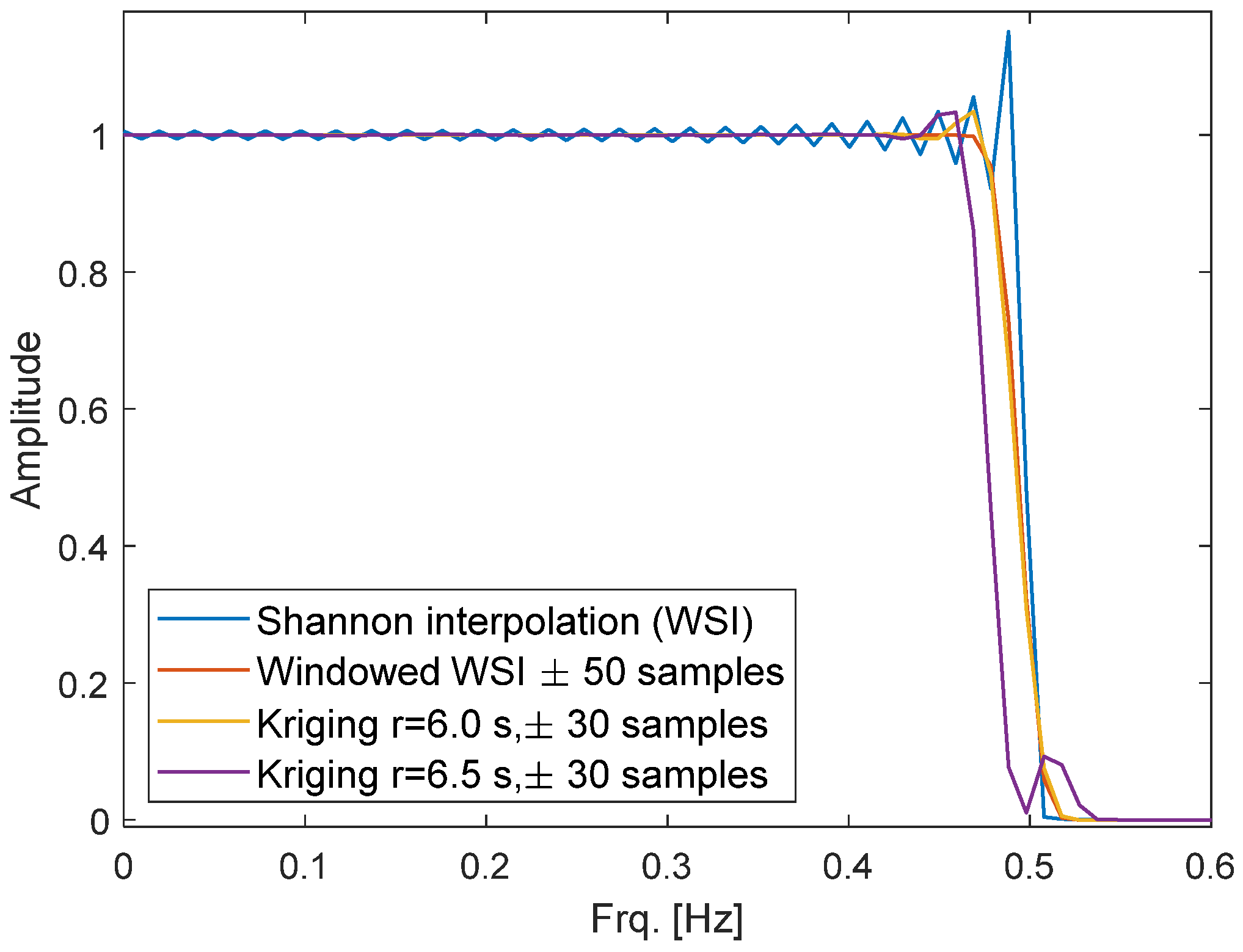
Initially, only uniform sampling in the group-delay scenario is examined. Kriging, Lagrange, and windowed WSI calculate the target value by a weighted sum of a limited number of input samples. Thus, they can be considered as FIR filter. To compare Kriging with WSI, the frequency response of the filters was evaluated using the following approach: A pulse function with T_S = 1 s and length of 103 samples was taken as input with y₅₁ = 1 and otherwise 0. The signal was reconstructed with a resolution of 0.1 s from the input. Its spectrum was calculated with a fast Fourier transform (FFT) of length 1024 (Figure 2).

WSI without a window function produced a sharp cut at 0.5 Hz, complying with the desired brick-wall characteristics. However, it also showed ripples in the pass band due to signal truncation. Applying a window of ±50 samples length significantly reduces the ripples, at the expense of a slightly less steep filter.

Different variogram types and parameters were tested for Kriging. A Gaussian variogram with r = 6·T_S, s = 1 and n_g = 0 produced a pulse response and filter characteristics that were nearly identical to those of the windowed WSI. Taking ±30 samples on either side of the target point was sufficient as inputs for Kriging.

When the range was increased to r ≥ 6.5 T_S, ripples appeared in the frequency response and the Kriging matrix became ill-conditioned for long input windows. Further testing will be presented in Section 4.

The standard method for defining the variogram model involves fitting the model to the estimated statistical properties of the input signal obtained experimentally, as we did in earlier publications [23,26]. The above-described method to tune the variogram model to achieve the desired FIR filter response is less common. Nevertheless, this method yielded accurate reconstructions for a wide range of input signals (Section 4). Notably, the reconstruction accuracy was better than that of WSI, particularly near the edges of time-limited signals.

The second case considers the extension to non-uniform sampling. It is assumed that the same variogram can be applied to this case because Kriging does not discern between uniform and non-uniform spaced inputs. In Section 4, we will evaluate this assumption and compare the performance of Kriging with Lagrange interpolation through simulation.

In the third case, which involves the single-delay scenario, the FIR filter is truncated and no longer symmetric. This prevents the use of standard methods for FIR filter design. Simulations show that the filter becomes noise sensitive (Section 4.3). Kriging provides solutions for both problems. The weights of the remaining filter taps are inherently corrected by filling the Kriging matrix with the remaining samples. The nugget value can be adjusted to the noise amplitude for reducing distortions. From the other variogram parameters, only the range was slightly increased.

3.2. Test and Reference Signals

The different resampling methods were tested with bandlimited noise and sine waves of 0.05 Hz < f_L < 0.5 Hz in steps of 0.01 Hz as inputs, which is equivalent to an OSR between 1 and 10. Sensor measurements were simulated for a time window from 0 to 200 s with T_S = 1 s. The reconstruction was compared with a reference signal, which was generated by the same sine function or noise process with a higher time resolution of 0.1 s. The bandlimited noise was generated by applying a sinc filter to a white Gaussian noise sequence.

For the non-uniform case, the sampling time points t_n were varied by an evenly distributed offset between −0.24 T_AV ≤ Δt_n ≤ 0.24 T_AV, complying with the Paley–Wiener–Levinson theorem (3). This timing sequence is called a ‘random jitter’ or simply ‘jitter’. Additional timing sequences were generated to produce a higher variation Δt_n, while still complying to the theorem. The second sequence ‘alternate jitter’ toggles the sign of random Δt_n with |Δt_n| ≤ 0.24 T_AV. The third ‘max jitter’ sequence also toggles the sign but with the maximum allowed value of constant |Δt_n| = 0.24 T_AV.

The case of missing samples in otherwise uniform sampling was also tested. Every 11th sample was deleted. The prime factor 11 was selected to avoid multiples of f_L. It should be noted that the missing sample case includes occasional ΔT = 2T_S and thus violated the theorem (3). Furthermore, the average interval increases to T_AV = 1.1·T_S. The Kriging range was increased by the same factor.

All inputs were scaled to 0 mean and variance of 1. In additional simulations, the stability of the reconstruction against noise and quantization caused by the ADC was tested.

3.3. Input Window for Interpolation Algorithms

The different interpolation methods were more stable and required less CPU time if the input was constrained to a time window. The window stretched from half window (HW) samples to the past and HW samples to the future. For the single-delay scenario, the same number of HW past samples, but only one future sample was included.

For windowed WSI and Lagrange good results were achieved with HW = 20. For Kriging, HW was set to 25 after testing different values (Section 4.1). Multiplication with a window function was not necessary as Kriging inherently applies weighting of the input samples.

3.4. Evaluation of Reconstruction Accuracy

The reconstruction accuracy was evaluated for Kriging and compared with Lagrange, Margolis, and Akima as reference methods. The root mean square error (RMSE) between the reconstructed signal and reference signal with a time resolution of 0.1 s was calculated as indicator value. The SNR for an input signal with σ = 1 is given by:

$$SNR=-20 lo{g}_{10}(\mathrm{RMSE}) \mathrm{dB}.$$

(12)

When reconstructing time-limited signals close to the Nyquist frequency, an error is unavoidable, especially when there are gaps in the signal longer than 3/f_L due to missing samples. The largest deviations occur at the edges of the measured time window. The RMSE was calculated separately for the first and last 5 s at the margins, and for the remaining centre of the measured window in the group-delay scenario. The single-delay scenario showed high errors for the first sensor samples, when neither future nor sufficient past samples were available. The first 10 s were therefore ignored in the RMSE calculation.

During a frequency swapping, the band limit f_L of the test signal was increased until the error became so high that the reconstruction was useless. The threshold for an acceptable error E_Max was set to RMSE = 0.01, which is equivalent to SNR = 40 dB. A higher SNR is possible but requires lower f_L or higher f_S. To assess the suitability of various resampling methods at high f_L, the maximum band limit f₄₀ was determined, which ensured the error remained below the threshold E_Max. Conversion to the OSR can be achieved using

$$\mathrm{OSR}=\frac{f_s}{2·f_{40}}.$$

(13)

The first round of simulations was carried out for the group-delay scenario. The bandlimited noise test signal produced lower errors compared to sine waves with the same f_L. The signal energy is evenly distributed over lower frequencies for the bandlimited noise. Tests were focused on the sine wave inputs as they represent the worst-case input.

3.5. Simulation Procedure

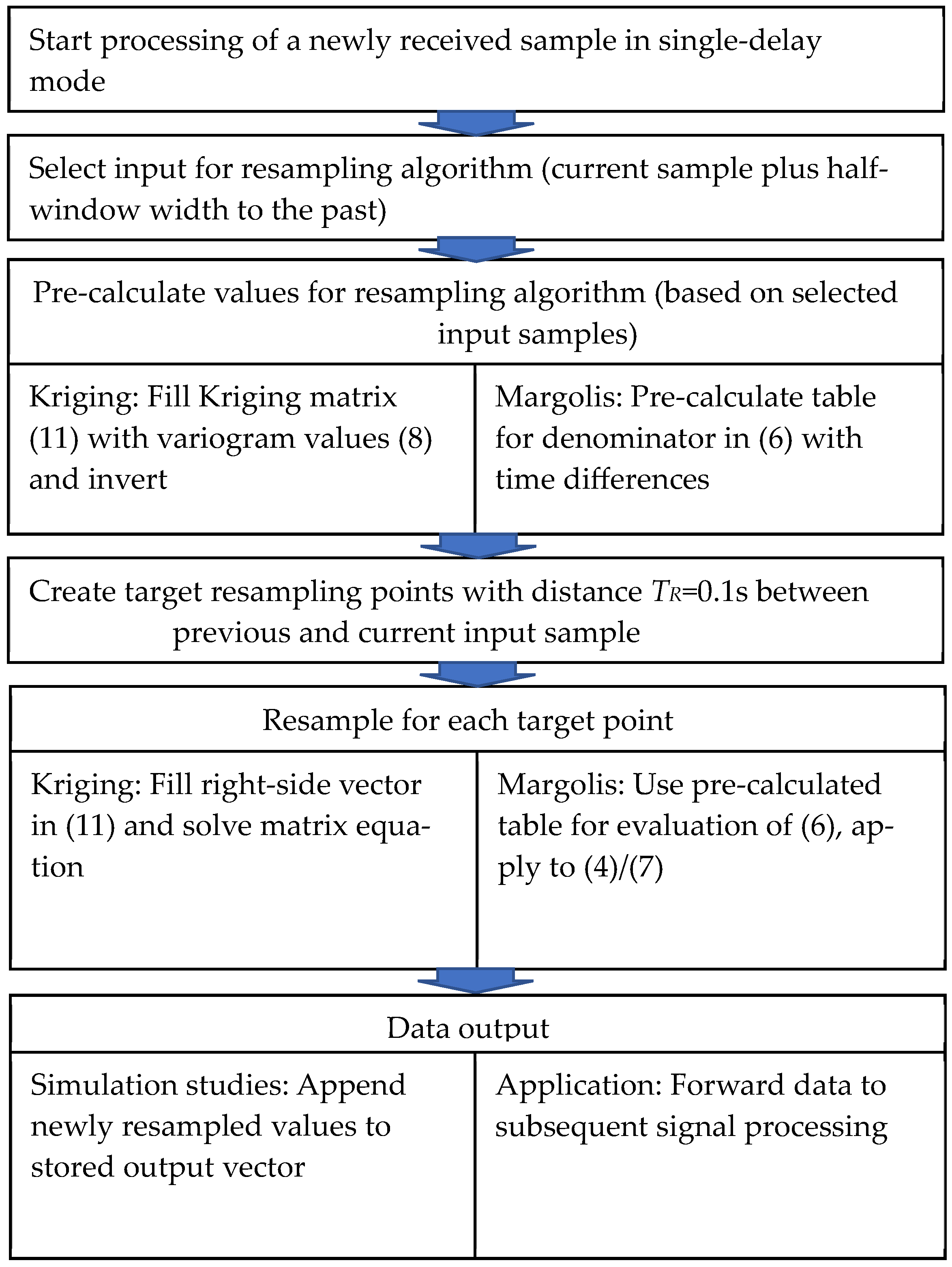
The single-delay scenario was simulated as an event-driven process that is triggered by the arrival of each new sample. The process reconstructs the signal for the time interval between the current and the previously received input sample. The newly reconstructed samples are appended to the stored reconstruction from the previous process runs.

The simulation procedure is shown as pseudo-code in Figure 3. After receiving a new sensor sample, the input window for the resampling algorithm is selected, containing the current and several past samples. If upsampling is required, i.e., multiple output samples must be calculated per input sample, code execution time can be largely reduced for Kriging and Margolis. The output points use all the same input samples with identical time differences between them. The left side matrix in (11) for Kriging remains constant, as well as the denominator in (6) for Margolis. The inversion of the Kriging matrix can be pre-calculated. An explicit call of QR-decomposition resulted in the same RMSE as calling the standard matrix inversion method ‘numpy.linalg.pinv’ in Python. Both options required similar processing time. For Margolis, the denominator values were pre-calculated and stored in a table.

The output samples were appended to a vector. The RMSE was calculated after all input samples were processed. Lagrange and Akima were tested by a similar procedure. The latter two algorithms with lower complexity did not require pre-calculation.

All simulations were programmed in Python. Simulation results were stored as JSON files and plotted in Matlab (See data attachment) or Supplementary Materials. The average required CPU time to reconstruct one sample was calculated from the total CPU time for reconstructing the whole reference signal with 2000 samples.

4. Results

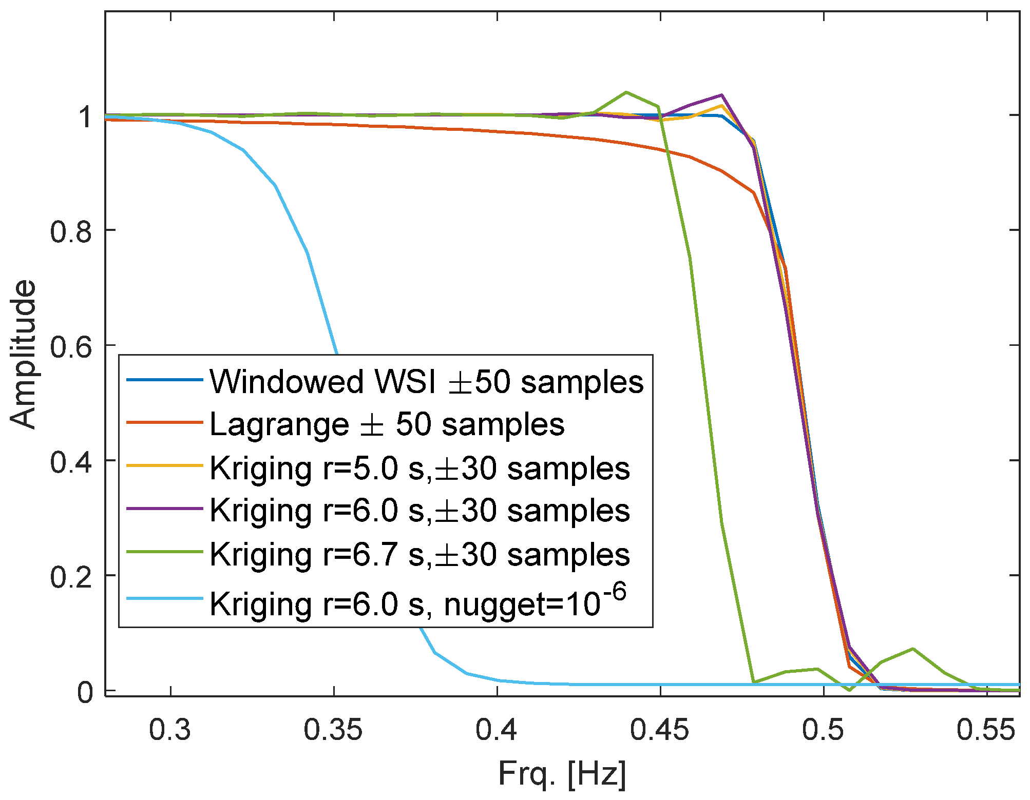
During the first test, the effect of the Kriging range and nugget value on the frequency response was evaluated according to the method described in Section 3.1. Even a small nugget of n_g = 10⁻⁶ has a significant effect on the frequency response (Figure 4). The corner frequency drops from 0.5 Hz to 0.35 Hz. Kriging with r = 5·T_S or r = 6·T_S has almost the same frequency response as windowed WSI. Higher range values create ripples and slightly decrease the corner frequency. The values r = 6·T_S and n_g = 0 were used as standard setting until further testing.

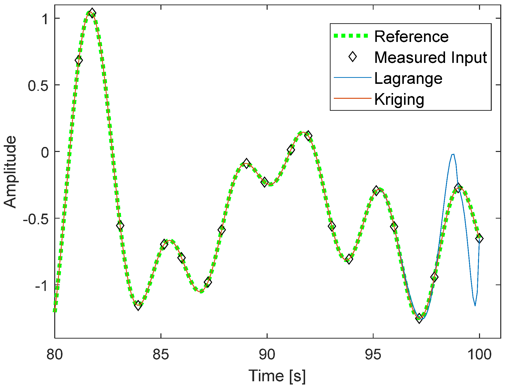
Figure 5 shows an example test signal with alternating jitter, generated by bandlimited noise with f_L = 0.3 Hz and reconstruction by Lagrange interpolation and by Kriging. The Kriging reconstruction had an RMSE of 0.0014 at the margins of the sampled time window and was nearly indistinguishable from the reference signal. On the other hand, Lagrange exhibited a significant deviation at the end of the time window, with an RMSE of 0.158.

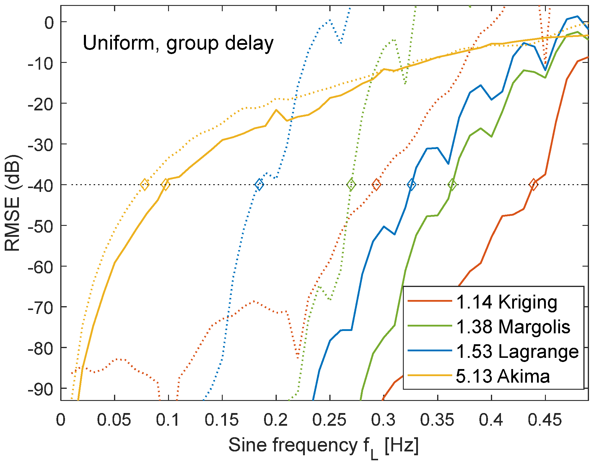
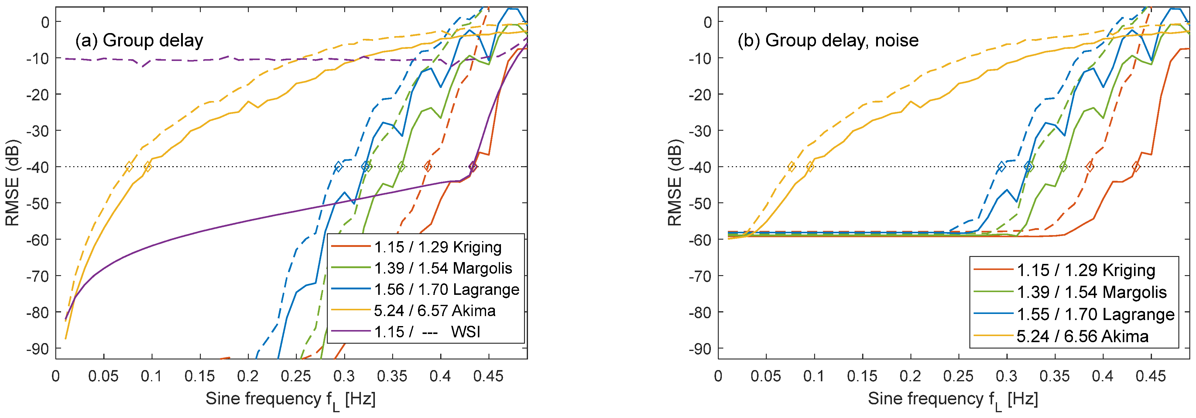
The process of frequency swapping to estimate f₄₀ with an RMSE below E_Max = −40 dB is illustrated in Figure 6 for the group-delay scenario with a uniform sine wave test signal. Intersections of the frequency diagram with the line for E_Max = 0.01 or −40 dB are marked by diamonds. The resulting OSR values for the centre of the available time window were calculated using (13) and listed in the legend. Kriging enables lower OSR compared to Margolis, Lagrange, and Akima. Akima has the advantage that it only requires a window of ±3 samples and thus provides the same stability at the margins. However, the RMSE was so high that it can only be applied to signals with a band limit below 0.1 Hz, which is equivalent to an OSR of 5. The other methods besides Akima were all highly sensitive to the insufficient number of input samples at the margins, leading to an increase of RMSE by a factor of more than 100, which must be compensated by higher OSR.

Sine wave input signals always produced a higher RMSE than bandlimited noise, resulting in lower f₄₀ values. Depending on the interpolation method, the required OSR was between 5% and 8% higher for sine waves, which were therefore considered as the worst-case scenario and used as standard input signals in the following tests.

The three different jitter modes produced almost the same f₄₀ values. The OSR varied by 2%. Random jitter was taken as the default in the subsequent tests.

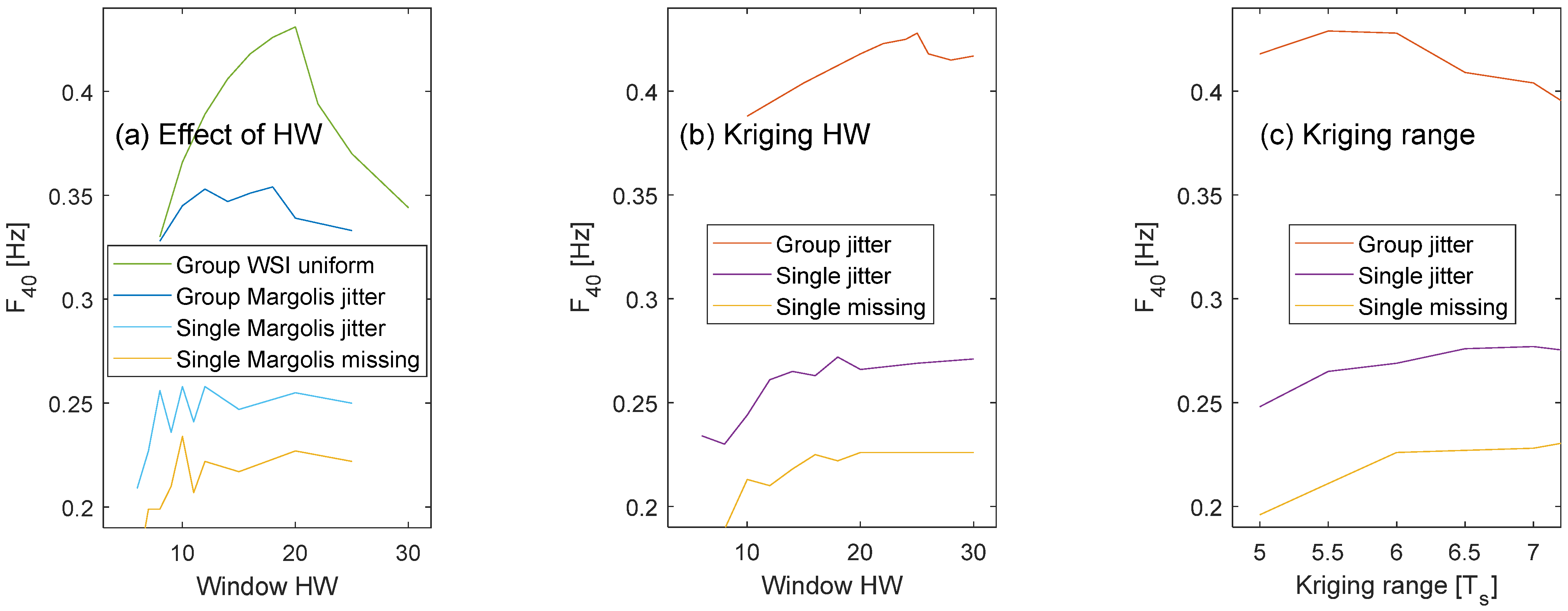
4.1. Influence of Window Length and Kriging Range

Additional simulations were also performed to evaluate the impact of the window half-width and Kriging range on f₄₀ (Figure 7). When selecting the values of HW and r other factors must also be considered, such as a flat frequency response, ensuring reasonable CPU time, and maintaining mathematical stability.

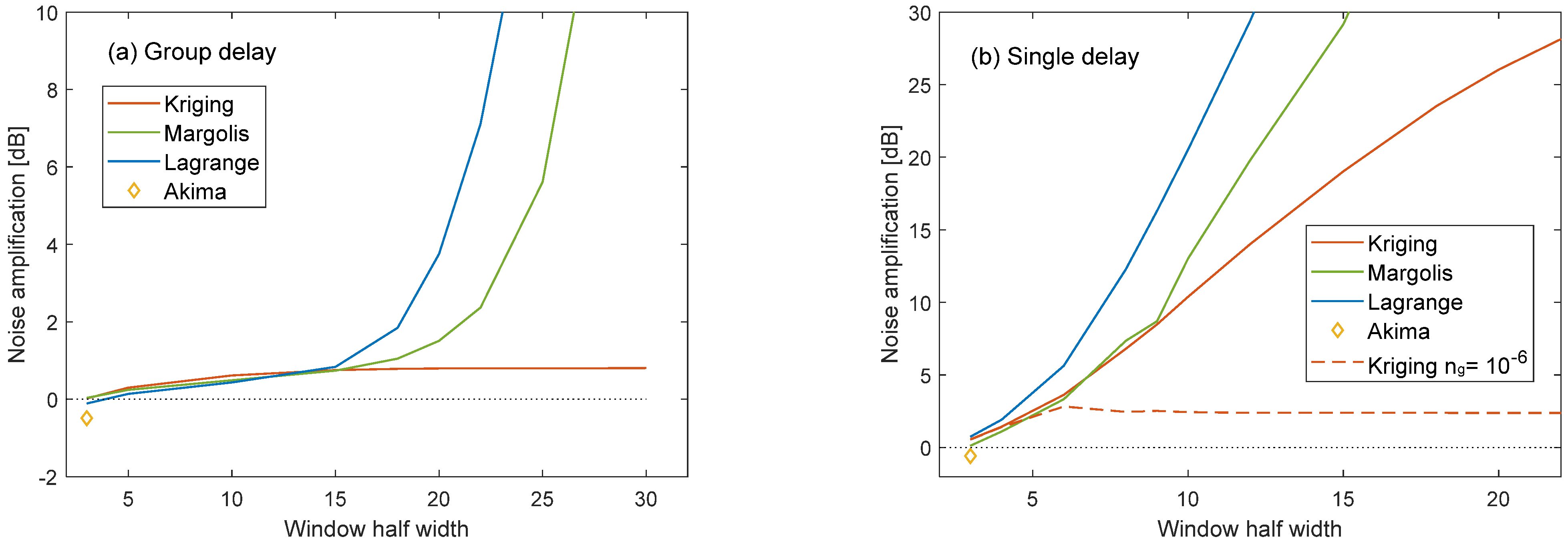
The noise sensitivity of the different methods was tested in additional simulations. White noise with σ = 1 was used as input signal. Depending on the resampling method and the window width, the output contained amplified noise and aliasing frequencies. The relation of the root mean square amplitudes (RMSA) between the resampled output signal and the noise input signal was calculated. The relation showed how distortions by noise are amplified by the different methods (Figure 8). Kriging was tested for two variogram parameter sets, including zero nugget and n_g = 10⁻⁶. Further analysis of the nugget follows in Section 4.4.

Akima was the only method that slightly reduced the noise amplitude by −0.6 dB. However, it can only operate with a fixed HW of three. The noise sensitivity of Margolis and Lagrange increased with the HW. Kriging provided an almost constant moderate noise amplification of 0.8 dB for group- and 2.4 dB for single-delay. The nugget value must be included in the variogram for the single-delay scenario; otherwise, the noise sensitivity also increases with HW for Kriging.

HW was set to the values with the highest f₄₀ for the group-delay scenario, i.e., HW = 20 for WSI, HW = 18 for Lagrange/Margolis, and HW = 25 for Kriging. Lower HW values are preferred for the single-delay scenario to reduce CPU time and noise sensitivity. Values of HW = 10 for Lagrange/Margolis and HW = 20 for Kriging were selected. These values also provided a good accuracy regarding a lower error threshold of E_Max = −60 dB. Margolis and Lagrange are both highly noise sensitive; higher HW values should be avoided. WSI did not yield satisfactory accuracy in the single-delay scenario regardless of HW.

The Kriging range was set to r = 6·T_S for the group-delay scenario. The higher average sampling interval of T_S = 1.1 s for the case of missing samples corresponds to r = 6.6 s. A slight increase of the range for the single-delay scenario to r = 6.5·T_S, equivalent to r = 6.5 s for uniform and jitter, and r = 7.15 s for missing samples, led to higher f₄₀ values.

4.2. Reconstruction Accuracy in the Group-Delay Scenario

The first set of simulations was carried out for the group-delay scenario, basically as reference for comparison with the single-delay scenario.

WSI provided better accuracy than Margolis, Lagrange, and Akima uniform input signals with a high band limit f_L > 0.4 Hz, and about the same accuracy as Kriging (Figure 9a). A SNR of 40 dB was achieved with OSR = 1.15. However, The RMSE declined only slightly for lower frequencies, for which WSI was outperformed by the other methods. Furthermore, WSI was highly sensitive towards distortions of the sample timing. It was impossible to achieve an RMSE below −10 dB if samples were missing. Therefore, WSI was excluded from the further tests.

The other methods were tested for jitter and missing samples. Kriging provided the lowest RMSE for all frequencies, followed by Margolis and Lagrange. For the missing samples test signal, every 11th or 9% of the samples were deleted. The RMSE increased accordingly (dashed lines) and required a 6% to 12% higher OSR.

Adding noise with RMSA = −60 dB did not significantly affect the OSR for E_Max = −40 dB (Figure 9b). The RMSE of all methods, except Akima, approached for f_L < 0.25 Hz the noise floor of −60 dB, with an offset between 0.8 dB (Kriging) and 1.9 dB (Lagrange). All methods proved to be stable towards noise in the group-delay scenario, although they did not provide additional noise smoothing capabilities.

Kriging was the most accurate method, for both clean and noisy input signals. The restriction to time-limited signals required slight oversampling with OSR = 1.15 to achieve SNR = 40 dB and OSR = 1.34 for SNR = 60 dB.

4.3. Single-Delay Scenario

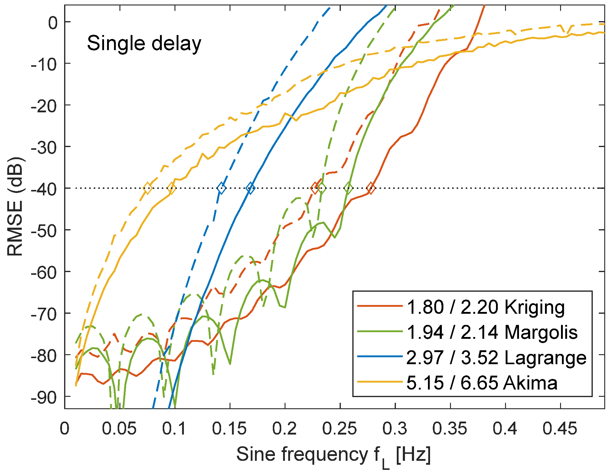
All methods, except for Akima, required higher OSR to achieve the same SNR, after switching to the single-delay scenario (Figure 10). Akima always required three future samples for both group- and single-delay scenarios. The other methods were only allowed to use one future sample.

The RMSE for Margolis showed significant oscillations, with negative peaks every 0.05 Hz. Margolis provides perfect reconstruction of recurrent signals, which explains the low error if the input window length is a multiple of the signal interval. The window length was defined in samples, which led to slightly varying length in time units in case of jitter. Therefore, an exact match with the signal interval and perfect reconstruction was not fully achieved.

Apart from those oscillations, Margolis and Kriging achieved similar RMSE values, with a slight advantage for Kriging at the threshold of E_Max = −40 dB. The necessary OSR to resample jitter signals by Kriging was 8% lower compared with Margolis, 39% compared with Lagrange, and 65% compared with Akima.

In comparison with the group-delay scenario, the OSR had to be increased by a factor of 1.4 for Margolis, by a factor of 1.6 or 1.7 for Kriging, and by a factor of 2 for Lagrange to achieve at the threshold of E_Max = −40 dB. For a threshold of −60 dB, a factor between 1.5 and 2.2 was necessary.

Comparing jitter and missing samples in the single-delay scenario showed that a between 10% and 22% higher OSR was necessary in the latter case. The percentage increase of the OSR was higher, as it also was in the group-delay scenario.

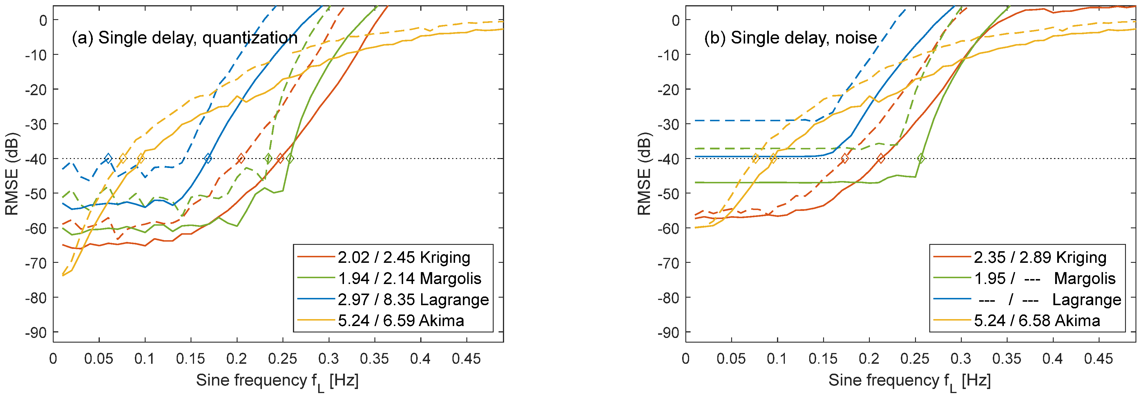
The OSR was only slightly increased by quantization (Figure 11a). Apart from this, the single-delay scenario was highly sensitive towards noise. If the input signal was truncated to a resolution of 12 bits, only Akima came close to the equivalent noise floor of −78.2 dB. The other methods had RMSE values between 12 dB and 23 dB above the input noise. In case of missing samples, it was not possible to achieve at a lower error threshold of E_Max = −60 dB.

If a higher noise amplitude of −60 dB was added to the input signal, Kriging and Margolis showed dissimilar behaviour (Figure 11b). Kriging was better for signals with lower frequencies with f_L < 0.19 Hz. The lowest RMSE values were 2.7 dB above the noise floor, whereas Margolis remained 13 dB above the noise floor. Above f_L > 0.19 Hz, Margolis was the more accurate method for jitter signals, with a 17% lower OSR. However, Margolis failed to provide satisfactory interpolation in case of missing samples. Only Kriging and Akima achieved at an RMSE below −40 dB.

4.4. Adjustment of the Nugget Value

The nugget value was already adjusted in Figure 11. In theory, the variogram nugget is equivalent to the squared mean amplitude of an additional white noise distortion (Section 2.7). For the single-delay scenario with noise, the nugget was set to n_g = 10⁻⁶ for noise with −60 dB RMSA and to n_g = 10⁻⁸ for 12-bit quantization. Kriging interpolation without nugget resulted in a significantly higher RMSE (Figure 12).

The single-delay scenario is highly sensitive towards white noise with spectral components above f_L. White noise with −60 dB RMSA pushes the RMSE to −25 dB for the missing samples case. After setting the nugget value, the RMSE dropped below E_Max = −40 dB for OSR > 2.89. Adding the nugget also reduced the filter corner frequency to 0.35 Hz (Figure 4). The single-delay scenario is not significantly affected because f₄₀ is below this corner frequency. However, adding a nugget to the group-delay case would reduce f₄₀, which has about the same value as the corner frequency. Furthermore, the group-delay scenario had already a low noise sensitivity of 0.8 dB (Figure 8). The use of the nugget is only recommended for the single-delay scenario.

4.5. Effect of Additional Future Samples

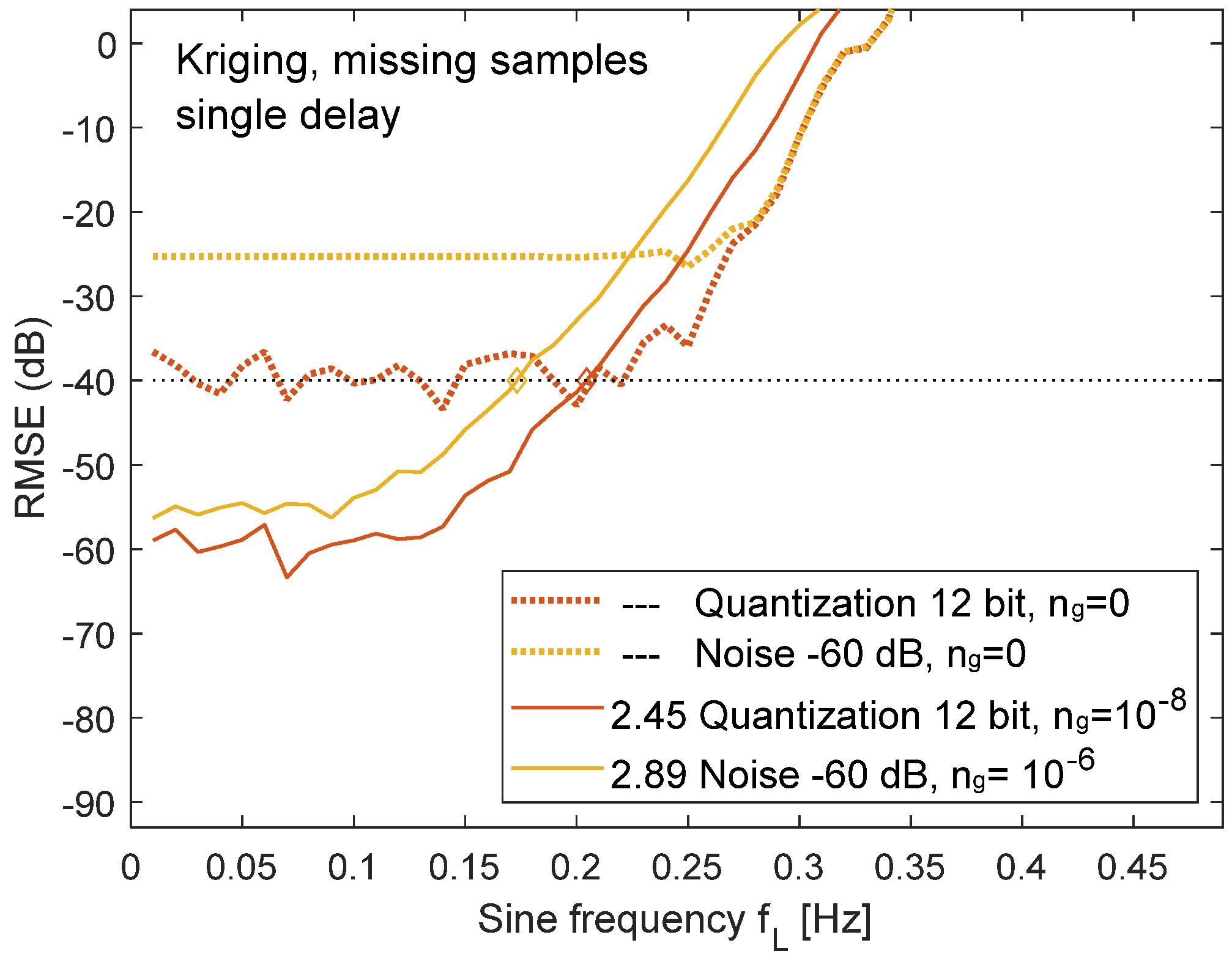
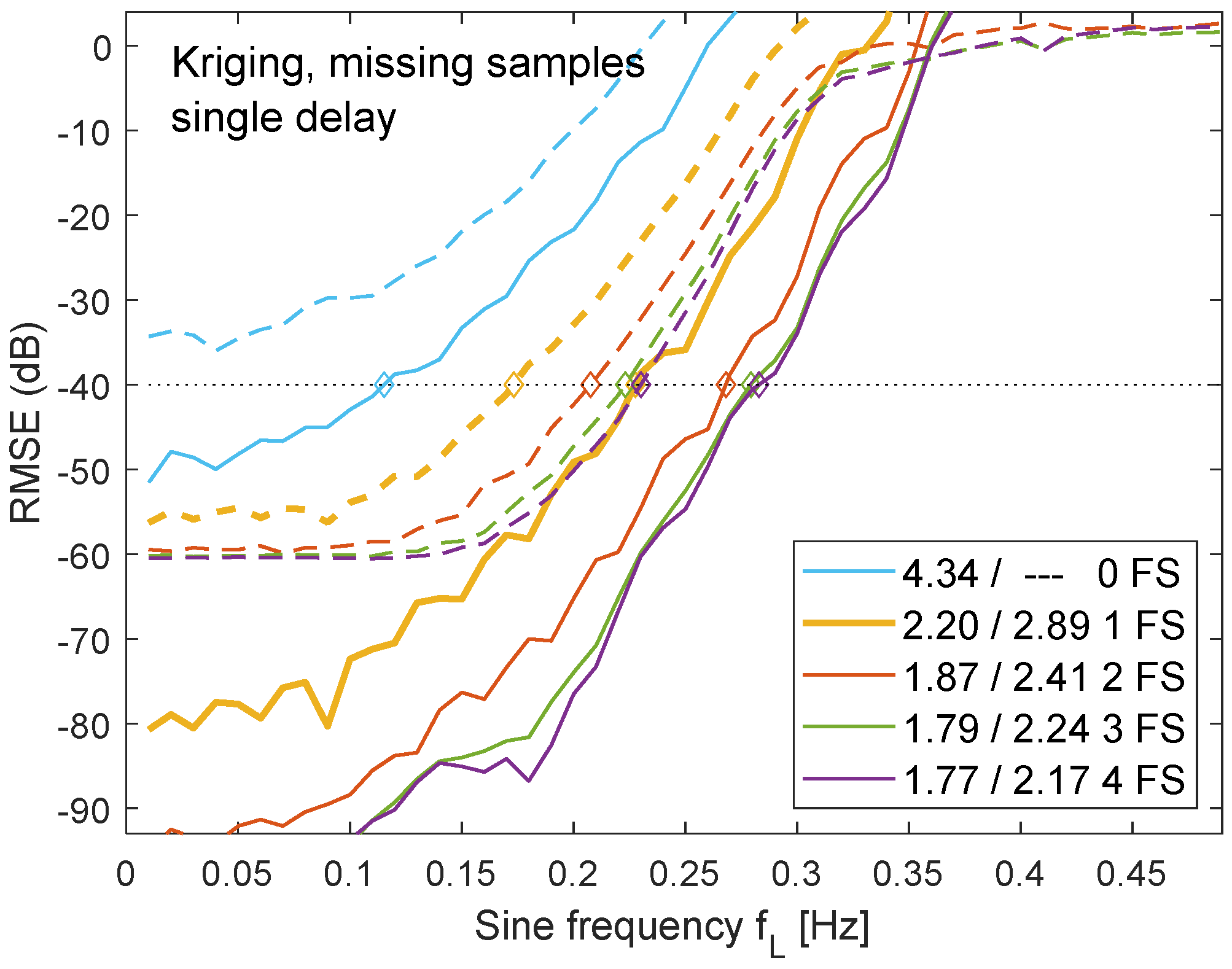
Missing samples were the most problematic case for the single-delay scenario. The RMSE can be reduced by providing more than a single future sample for the reconstruction algorithm (Figure 13). Taking a second future sample for the noisy test signal improved the OSR by 18%, a third future sample by 23%. Adding a fourth future sample brought only marginal advantage. Margolis profited less from additional future samples with only 7% improvement by using three future samples. The case of three future samples corresponds to Akima with a fixed input window of ±3 samples. Allowing 25 future samples would be identical to the group-delay scenario. The number of future samples that can be used depends on the acceptable group delay in the related application.

In case of zero future samples, a prediction for the current point of time is calculated before the next input sample becomes available. The prediction requires extrapolation instead of interpolation. The prediction error largely increases and requires the double OSR = 4.34. In case an input signal with missing samples and noise, the threshold of −40 dB was not achieved without future samples.

4.6. Required CPU Time for Reconstruction

The required CPU time for calculation of the reconstructed signal was measured on a workstation with an Intel i7-4790 processor with four cores, 3.60 GHz clock speed, and 32 GB memory. The average time for reconstructing one output sample t_CPU in a time resolution of 0.1 s was calculated from the total time required to reconstruct 1000 output samples (

Table 1. Required CPU time for pre-calculation and total average (including pre-calculation).

Method	Pre-Calculation Time tPRE per Input Sample		Total CPU Time tCPU Per Output Sample
	Group Delay	Single Delay	Group Delay	Single Delay
Kriging	3 ms	0.5 ms	380 μs	100 μs
Margolis	1 ms	0.15 ms	620 μs	85 μs
Lagrange	-		470 μs	55 μs
Akima	-		20 μs

).

Kriging and Margolis both used pre-calculation to reduce CPU time. The inverse Kriging matrix (11) and a table for the denominator in (6) was calculated once per input sample and applied to ten output samples, as described in Section 3.5. The average CPU time per output sample was 380 μs for Kriging (HW = 25) and 620 μs (HW = 18) for Margolis including pre-calculation. The pre-calculation caused peaks of t_PRE = 3 ms for Kriging and t_PRE = 1 ms for Margolis.

Due to the required matrix inversion, the pre-calculation for Kriging has the higher complexity of O(n³). Margolis requires the evaluation of n² terms in Equation (6) with O(n²). Both algorithms have the same complexity of O(n²) for the additional operations per output sample, either for multiplying the inverted Kriging matrix with the vector on the right side of (11), or for evaluation of the numerator in (6). The latter one is more expensive due to the sine function, leading to a higher total t_CPU for Margolis.

The single-delay scenario required less CPU time because the HW was lower and only HW past and one future sample were processed. The matrix order was reduced by a factor of almost two. Margolis provided slightly faster processing with t_CPU = 85 μs (HW = 10), compared with Kriging with t_CPU = 100 μs (HW = 20). The pre-calculation time reduced to t_PRE = 0.5 ms for Kriging and t_PRE = 0.15 ms for Margolis.

In case of a regular sampling pattern, e.g., uniform sampling or periodic jitter, the pre-calculation must be carried out only once. Afterwards, it does not contribute to the average t_CPU, which than drops to 50 μs for Kriging and 70 μs for Margolis.

Akima took in both scenarios ±3 input samples and required the same t_CPU = 20 μs for group and single delay.

5. Discussion

The results are discussed regarding the main questions of this contribution, i.e., the problems and feasibility of single-delay resampling and the performance of the new Kriging approach.

5.1. Challenges in Single-Delay Resampling

Most resampling algorithms use a symmetrical time-limited window from the input signal to calculate the reconstruction. As a result, the output is only available after a certain group delay, which may be acceptable in the target application. With this approach, a high SNR can be achieved with a low OSR (

Table 2. Necessary OSR for different test cases. All OSR values achieved by Kriging if not stated otherwise.

Test Case	SNR	Noise	Necessary OSR/by Method
			Group-Delay	Single-Delay
Jitter	40 dB	-	1.15	1.80
Jitter	40 dB	−60 dB	1.15	1.95/Margolis
Jitter	60 dB	-	1.34	2.40
Missing samples	40 dB	-	1.29	2.14/Margolis
Missing samples	40 dB	−60 dB	1.29	2.89
Missing samples	60 dB	-	1.42	3.09

). A jitter within the limits of theorem (3) and noise with RMSA = −60 dB had minimal impact in the group-delay scenario. When every 11th sample was missing, the necessary OSR typically increased by 10%, which can be attributed to the higher average sampling interval.

Only a few methods can reconstruct the signal without waiting for future samples or recalculate filter coefficients, if the filter is truncated. Methods based on complex optimization were also excluded for the processing of live sensor data. Kriging, Margolis, and Lagrange calculate the weighting factors based on the available set of input samples and can thus adapt to an unsymmetrical, truncated set.

The restriction to the single-delay scenario required an increased OSR by a factor between 1.6 and 2.2 (Table 2). Furthermore, all methods, except Akima, became noise sensitive. Only moderate noise amplification was observed up to a window half width of HW = 18 in the group delay scenario, whereas the noise for Margolis and Lagrange sharply increased even for small HW values in the single-delay scenario (Figure 8).

The high noise sensitivity in the single-delay scenario can also be explained by Figure 10. Input signals above f_L~0.3 Hz result in an RMSE > 0, i.e., the distortion is larger than the input signal. High spectral components of noise signals lead to amplified distortions in a similar way.

The combination of missing samples and noise was the most difficult case. Only Kriging and Akima achieved at SNR = 40 dB, with the latter one requiring a high OSR = 6.58. At least one future sample must be available to avoid exceedingly high prediction errors.

5.2. Performance of Kriging

All reconstruction methods take assumptions about the input signal, mostly that the signal is bandlimited and time-infinite or periodic. If the assumptions are fully met, perfect reconstruction is feasible. Kriging assumes that the signal originates from a statistical process, and therefore does not provide perfect reconstruction, but the best possible estimate, the so-called best linear unbiased estimator (BLUE) [23]. This BLUE property is only achieved if the variance of the process over time or space depends only on the variogram.

In practise, these assumptions cannot be fully met. Either the signal is time-limited, or, in the case of Kriging, there is only a raw estimation for the variogram available from limited experimental data. Variogram parameters are normally estimated in the time domain, however, the settings of the variogram to achieve a good frequency response, as described in this paper (Section 3.5 and Section 4.4), led to highly accurate reconstructions in the group-delay scenario.

In the single-delay scenario, the weighting of the input samples can no longer be interpreted as symmetric filter. Kriging was developed as a space- or time-domain interpolator. As such, Kriging provides good interpolation, even if design in the frequency domain is no longer feasible after filter symmetry is lost due to truncation of the input window.

As a statistical method, Kriging is suitable for handling noise in both scenarios (Figure 8). Distortions are mainly caused by high-frequency components of the noise. The contribution of the spectral components of the noise can be estimated based on the RMSE caused by different sine frequencies (Figure 11b). The amplification of noise distortions by Kriging with f_L > 0.3 Hz is limited to 4 dB or a factor of 1.6 in the single-delay scenario (Figure 11b), whereas high frequency noise distortions are amplified by up to 21 dB for Margolis and 28 dB for Lagrange (beyond plotting scale in Figure 11b).

Kriging is the only method that can make use of a higher number of input samples by increasing HW, without increasing its noise sensitive at the same time. This noise stability requires to set the nugget value in the single-delay scenario (Section 4.4) with the disadvantage that the corner frequency of the equivalent filter is reduced (Figure 4).

5.3. Comparison with Other Methods

Kriging was the best of the four tested methods in the group-delay scenario, regarding all test cases including jitter, missing samples, noise, and higher SNR. Margolis and Kriging provided similar simulations results for noise-free signals in the single-delay scenario (Figure 10). If noise is added, Margolis is the more accurate method for f_L > 0.18 Hz. For lower frequencies, the RMSE remained above −47 dB, and Kriging provided more accuracy (Figure 11b).

The required CPU time was similar for both methods. It remained below 1 ms including additional pre-calculations once per input sample. Both methods are suitable for real-time applications.

Kriging was the least noise-sensitive method and the only one that could provide an RMSE below −50 dB for the case of missing samples combined with noise. However, Kriging has the disadvantage that two additional parameters must be set correctly. The variogram range can be set to a fixed value of r = 6·T_s or r = 6.5·T_s, depending on the scenario. The nugget value must be adapted to the actual noise of the signal.

Akima should only be applied if a band limit to f₀ < 0.1 Hz, or an OSR > 5 is acceptable and the signal contains high noise above the tested RMSA = −60 dB.

The comparison of Kriging was limited to three reference methods. Dedicated optimization methods might provide higher accuracy, e.g., compressed sensing assumes that the signal contains only a limited number of spectral components or wavelets. Such methods require high computations resources, mostly beyond the limitations of real-time processing.

Furthermore, the accuracy of Kriging might be improved by manually fitting of the variogram to a specific input signal. However, such fitting is only feasible, if the statistical properties of the signal do not change over time and if a large set of recorded sample data is available.

6. Summary

Kriging provided the best accuracy in the group-delay scenario. The OSR was reduced by 17%, 26%, and 78% compared with Margolis, Lagrange, and Akima. Kriging was the least noise sensitive method. The presented approach to set the variogram parameters according to the desired filter response was justified by the simulation results.

Wireless sensors send their data in intervals of seconds or minutes. Some transmissions might be lost or delayed. The slow interval allows for more demanding signal processing. However, delays caused by algorithms, which must collect several samples before a prediction for the current point of time can be calculated, are not acceptable. This leads to the demand for low-latency or single-delay resampling. The gap between the current and the previous sample should be reconstructed as soon as a new measurement arrives. Objectives include low OSR, low prediction error, and low latency. Not all of them can be achieved at the same time. In general, a higher RMSE or lower SNR must be accepted.

With Kriging and Margolis, two methods are available for resampling in the single-delay scenario. The restriction to past samples comes at a price. The OSR must be almost doubled to achieve the same SNR (Table 2). For the case of noise-free jitter input signals, Kriging was also the best method with an OSR reduction of 7%, 39%, and 65% compared with Margolis, Lagrange, and Akima. In case of missing samples Margolis was slightly better with a 4% lower OSR. Noisy jitter signals with f_L > 0.18 Hz were the second case, in which Margolis was better than Kriging. In all other cases, especially for noisy signals with missing samples, Kriging provided the more accurate resampling.

The simulations for Kriging and Margolis showed that single-delay resampling is feasible. Data from wireless sensors can be integrated with subsequent processing, e.g., by digital twins [4], even if the sensor timing is distorted by jitter or missing samples.