Hyperparameter Optimization Using Successive Halving with Greedy Cross Validation

Abstract

Training and evaluating the performance of many competing Artificial Intelligence (AI)/Machine Learning (ML) models can be very time-consuming and expensive. Furthermore, the costs associated with this hyperparameter optimization task grow exponentially when cross validation is used during the model selection process. Finding ways of quickly identifying high-performing models when conducting hyperparameter optimization with cross validation is hence an important problem in AI/ML research. Among the proposed methods of accelerating hyperparameter optimization, successive halving has emerged as a popular, state-of-the-art early stopping algorithm. Concurrently, recent work on cross validation has yielded a greedy cross validation algorithm that prioritizes the most promising candidate AI/ML models during the early stages of the model selection process. The current paper proposes a greedy successive halving algorithm in which greedy cross validation is integrated into successive halving. An extensive series of experiments is then conducted to evaluate the comparative performance of the proposed greedy successive halving algorithm. The results show that the quality of the AI/ML models selected by the greedy successive halving algorithm is statistically identical to those selected by standard successive halving, but that greedy successive halving is typically more than 3.5 times faster than standard successive halving.

1. Introduction

Artificial Intelligence (AI) and Machine Learning (ML) practitioners typically need to train and evaluate the performance of many different candidate models when developing an AI/ML-based solution [1,2]. The term model as it is being used here refers to the combination of a particular ML algorithm (e.g., linear regression, random forests, neural networks, etc.) and the vector of values to use for the algorithm’s hyperparameters, which are configurable settings that affect or control the learning process [3]. Such hyperparameters may be algorithmic (e.g., the choice of optimizer or the learning rate), or they may define the structure of an ML model itself (e.g., the number of hidden layers or nodes per layer in a deep neural network). The process of generating a candidate ML model is conceptually illustrated in Figure 1.

The art and science of searching for the combination of hyperparameter settings that yields the best-performing ML model is known as hyperparameter optimization [1], and it is this activity that resides at the core of the current paper. Using hyperparameter optimization is standard practice when developing ML-based solutions since no single ML algorithm or set of hyperparameter values will perform best in all use cases or with all datasets [4,5].

When performed competently, hyperparameter optimization identifies an ML model that yields optimal or near-optimal performance. Such an outcome has many obvious benefits, particularly in competitive contexts such as business or national defense. Nevertheless, hyperparameter optimization is plagued by a set of ubiquitous problems. First, many hyperparameters are real-valued. This suggests that there are often an infinite number of possible models in a given ML scenario, which makes it mathematically impossible to conduct an exhaustive search for an optimal model. Although training and evaluating an infinite number of candidate models is not possible, it is feasible to consider a large, finite set of models. Using hyperparameter optimization to train and evaluate the comparative performance of hundreds or thousands of candidate ML models can, however, be very time-consuming and expensive, particularly in the era of big data wherein training just one model may take hours or days [6]. Finally, training and evaluating ML models commonly relies on cross validation (discussed later), which can exponentially increase the time and costs associated with hyperparameter optimization [7]. In light of these considerations, AI/ML practitioners often find themselves in an awkward situation: on the one hand, hyperparameter optimization must be used to find the best-performing model possible given the available budget, but on the other hand, hyperparameter optimization can be both very expensive and very time consuming, and no researcher or organization is blessed with an infinite budget. Finding methods of reducing the time and other costs associated with hyperparameter optimization is therefore of great interest to the AI/ML community [8].

1.1. Successive Halving

Given the time and cost savings that can be realized via rapid hyperparameter optimization, it is perhaps not surprising that a variety of algorithms have been proposed with a view toward accelerating the hyperparameter optimization process [1,9,10,11,12,13,14]. Notable among these algorithms is a technique known as successive halving [11], which features prominently in the current study. In brief, successive halving is an iterative hyperparameter optimization method in which the number of candidate models decreases exponentially from one iteration to the next, while the number of training cases increases exponentially from one iteration to the next. The general strategy employed by the successive halving algorithm to quickly evaluate a set of candidate models is very similar to a single-elimination tournament. To begin, the algorithm uses a small number of training cases to quickly identify and cull unpromising candidate models. Models that survive to the next round are evaluated more thoroughly by using a larger proportion of the available data. This process repeats until only a few candidate models remain, which are then trained and evaluated using all of the available data.

Successive halving is classified as an early stopping-based approach to hyperparameter optimization because it abandons almost all candidate models without having trained or evaluated them using the complete set of training data. Successive halving has become quite popular due to its state-of-the-art performance and its recent inclusion in Python’s widely used scikit-learn machine learning library (implemented as the HalvingGridSearchCV and HalvingRandomSearchCV hyperparameter optimizers) [15]. An illustrative example of successive halving is depicted graphically in Figure 2 below, and a complete description of the successive halving algorithm can be found in Jamieson and Talwalkar [11].

1.2. Evaluating ML Model Performance Using Standard k-Fold Cross Validation

As noted previously, training and evaluating ML models commonly relies on a process known as cross validation. In standard k-fold cross validation, the available training data are split into k groups of approximately equal size (called folds). Each fold is then iteratively used as a testing set to evaluate a candidate ML model that has been trained using the remaining k-1 folds of training data [16]. After k model evaluation cycles, each fold will have been used as a testing set exactly once. The overall performance of the candidate model can then be quantified as the mean of the performance measurements obtained from each of the k model evaluation cycles. In addition to its ability to reveal problems with selection bias and overfitting, k-fold cross validation is commonly used when evaluating ML models because it provides insights into how well each candidate model will perform in the real world when it encounters input data that were not used during training. Standard k-fold cross validation also maximizes the value of the available training data by allowing every training case to be used for both training and testing in a statistically defensible way. These advantages notwithstanding, k-fold cross validation requires each candidate model to be trained and tested k times, thus exponentially increasing the total amount of work that is required to complete the overall hyperparameter optimization process. The standard k-fold cross validation process (with k = 5 folds) is shown in Figure 3.

1.3. The Role of Standard Cross Validation in Hyperparameter Optimization

Many methods of performing rapid hyperparameter optimization have been proposed, including Bayesian methods [13], early stopping methods [11,12], evolutionary methods [14], hypergradient methods [9,10], and greedy cross validation [8], among others. Regardless of the specific approach taken, the goal of each of these methods is to identify an optimal or near-optimal ML model as quickly as possible. Except for greedy cross validation (discussed shortly), all of these hyperparameter methods treat cross validation as a “black box” process. Put differently, these methods are only interested in the output of the cross-validation process—which is typically a measurement of a candidate model’s overall performance—without caring about how that output was generated. An example of standard cross validation being used as a black-box process in the milieu of the successive halving algorithm is illustrated in Figure 4 below. Although this figure focuses specifically on successive halving, comparable figures could be readily drawn to illustrate how cross validation is similarly used as a black-box process by other hyperparameter optimization algorithms.

1.4. Greedy Cross Validation

Greedy cross validation is a recently developed method that uses a modified version of cross validation in conjunction with partial performance metrics to focus resources on the most promising candidate models during the early stages of the hyperparameter optimization process [8]. In contrast to other hyperparameter optimization algorithms, greedy cross validation capitalizes on what is happening inside the “black box”. Recall that standard cross validation considers one candidate model at a time, sequentially evaluating all of the model’s folds before calculating the model’s overall performance metric and then proceeding to the next model [16]. Instead of completely considering one ML model at a time, greedy cross validation begins by first evaluating one fold for each of the candidate models being considered (as used herein, “evaluating a fold” means using the specified fold to test the performance of an ML model that has been trained using the remaining folds. Fully evaluating a model thus requires the evaluation of k folds). This process yields a partial performance metric for each ML model that represents the current best estimate of the model’s overall quality. From this point forward, the greedy cross validation algorithm always greedily pursues the most promising available option by evaluating the next fold for whichever candidate model currently has the best-known level of performance. After evaluating a fold, the current mean performance for the fold’s corresponding candidate model is updated, after which the algorithm again pursues the most promising available option. This process continues until either all of the folds for all of the candidate ML models have been evaluated, or until a stopping criterion (such as a time limit or the exhaustion of a computational budget) has been reached [8]. In this way, greedy cross validation directs computational resources to the most promising candidate models early in the search process and will typically complete a full evaluation of the best-performing ML models long before completing its evaluation of the worst-performing models. An illustrative example of greedy cross validation is provided in Figure 5 and a complete description of the greedy cross validation algorithm can be found in Soper [8].

1.5. The Path Ahead

The preceding discussion introduced hyperparameter optimization, successive halving, and the standard and greedy k-fold cross validation methods, all of which are essential foundation stones upon which the primary contributions of this paper will be built. In brief, the following sections of this paper are dedicated to developing and rigorously evaluating a new hyperparameter optimization algorithm that integrates greedy cross validation and successive halving. Given the critical need among AI/ML practitioners for fast and effective hyperparameter optimization methods, the primary goal of this new algorithm is to be able to select ML models of the same quality as those selected by successive halving but to do so much more quickly. Put differently, this research seeks to develop a greedy successive halving algorithm that is equivalent to standard successive halving in terms of its ability to select high-quality ML models, but which requires much less time than standard successive halving to perform that ML model selection task. Since standard successive halving is a very popular, state-of-the-art early stopping method for performing hyperparameter optimization, a new algorithm that can be rigorously shown to outperform standard successive halving would represent a noteworthy contribution to the AI/ML community. The balance of this paper seeks to make just such a contribution.

2. Materials and Methods

This section begins by introducing the greedy successive halving algorithm, which demonstrates how greedy cross validation can be integrated into the successive halving process. Successive halving ordinarily relies on standard cross validation, which treats ML model evaluation as an opaque “black box” process. The proposed greedy successive halving algorithm, however, relies on greedy cross validation, thus allowing the algorithm to pay attention to and benefit from the information that is generated while the ML model evaluation process is still underway. The greedy successive halving algorithm leverages this informational advantage to significantly increase the speed of the ML model selection process without sacrificing the quality of the models that are ultimately chosen.

After introducing the greedy successive halving algorithm, this section next describes the series of experiments that were conducted in order to compare the performance of the proposed algorithm against that of successive halving with standard cross validation, both in terms of wall-clock time and in the quality of the final ML models chosen by each algorithm. These experiments involve a variety of real-world datasets, a variety of machine learning algorithms (including both multiple classifiers and multiple regressors), differing numbers of folds for the cross-validation process, and differing sizes for the sets of candidate models that are considered by the competing algorithms. The results of these experiments—which reveal the overwhelming superiority of the greedy successive halving algorithm—are subsequently presented in Section 3.

2.1. The Greedy Successive Halving Algorithm

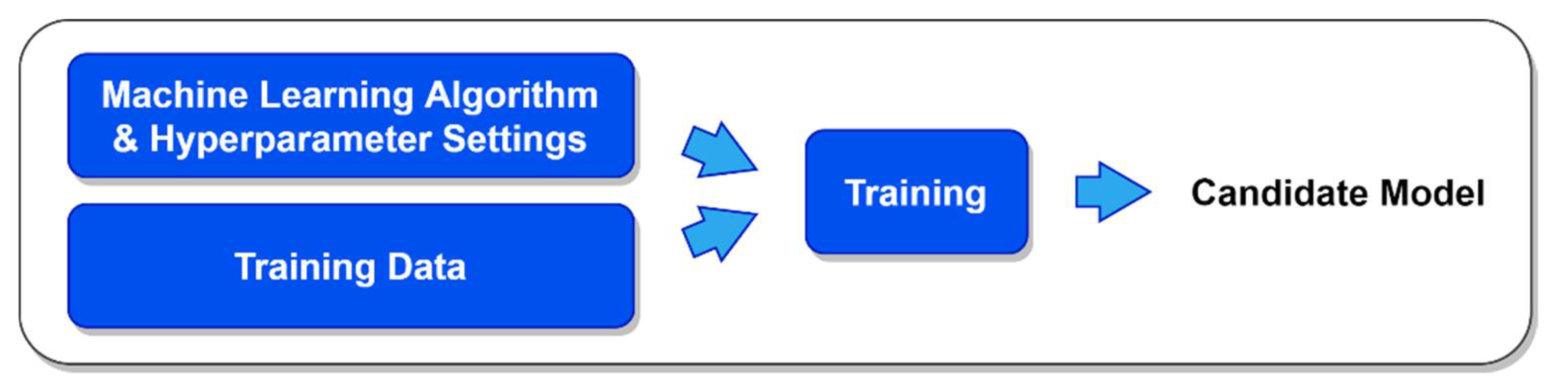
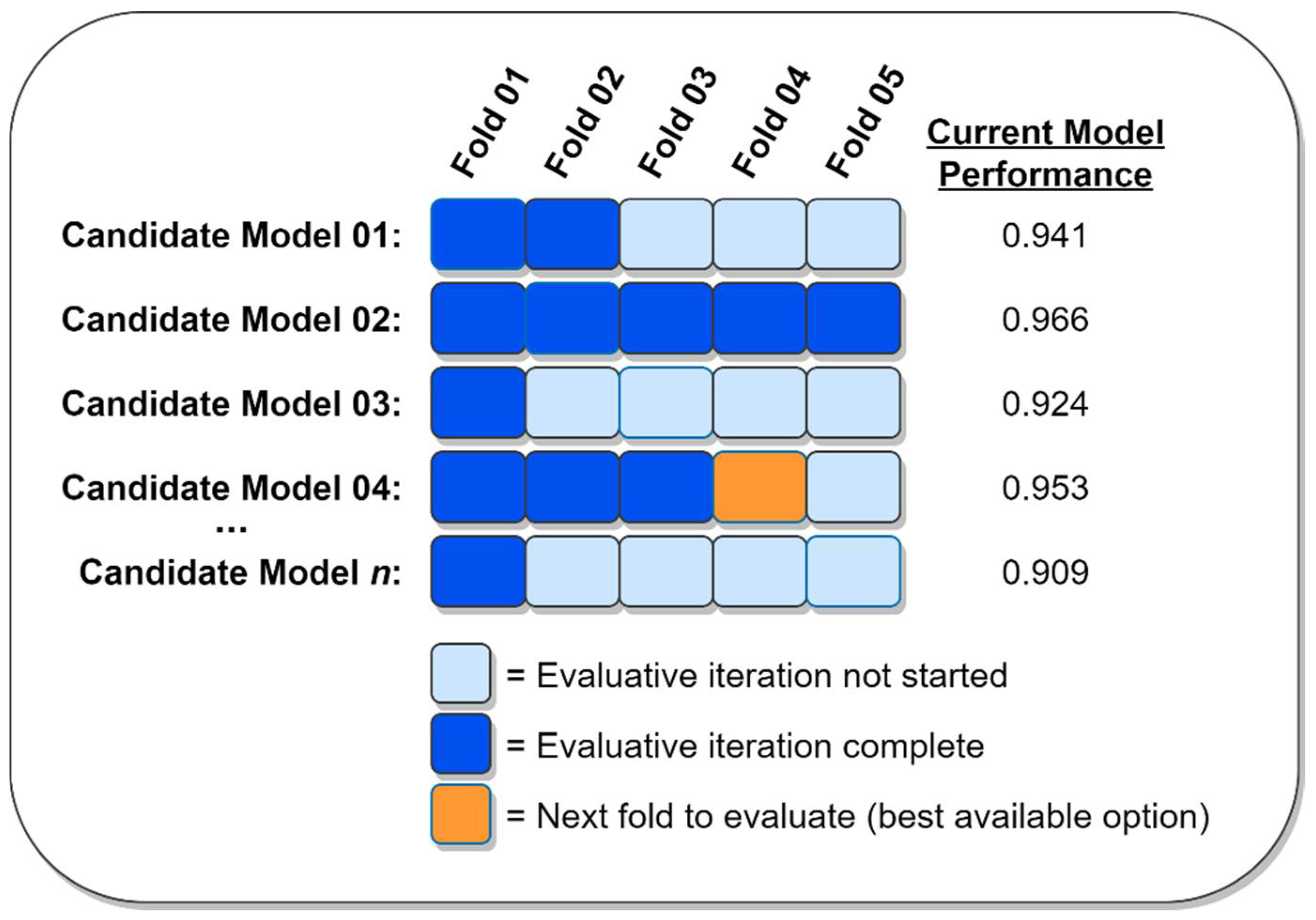
By design, standard cross validation fully evaluates each candidate ML model from start to finish and returns the model’s overall level of performance [16]. Standard cross validation is a memoryless process insofar as it neither cares about nor pays attention to how the performance of any candidate ML model compares to that of any other model. In contrast, greedy cross validation maintains an estimate of every candidate model’s level of performance and uses that information to prioritize the evaluation of the most promising models. This means that when using greedy cross validation, the most promising models will be the earliest to be completely evaluated during the overall model evaluation process [8]. The proposed greedy successive halving algorithm capitalizes on this difference between standard and greedy cross validation to achieve its superior performance.

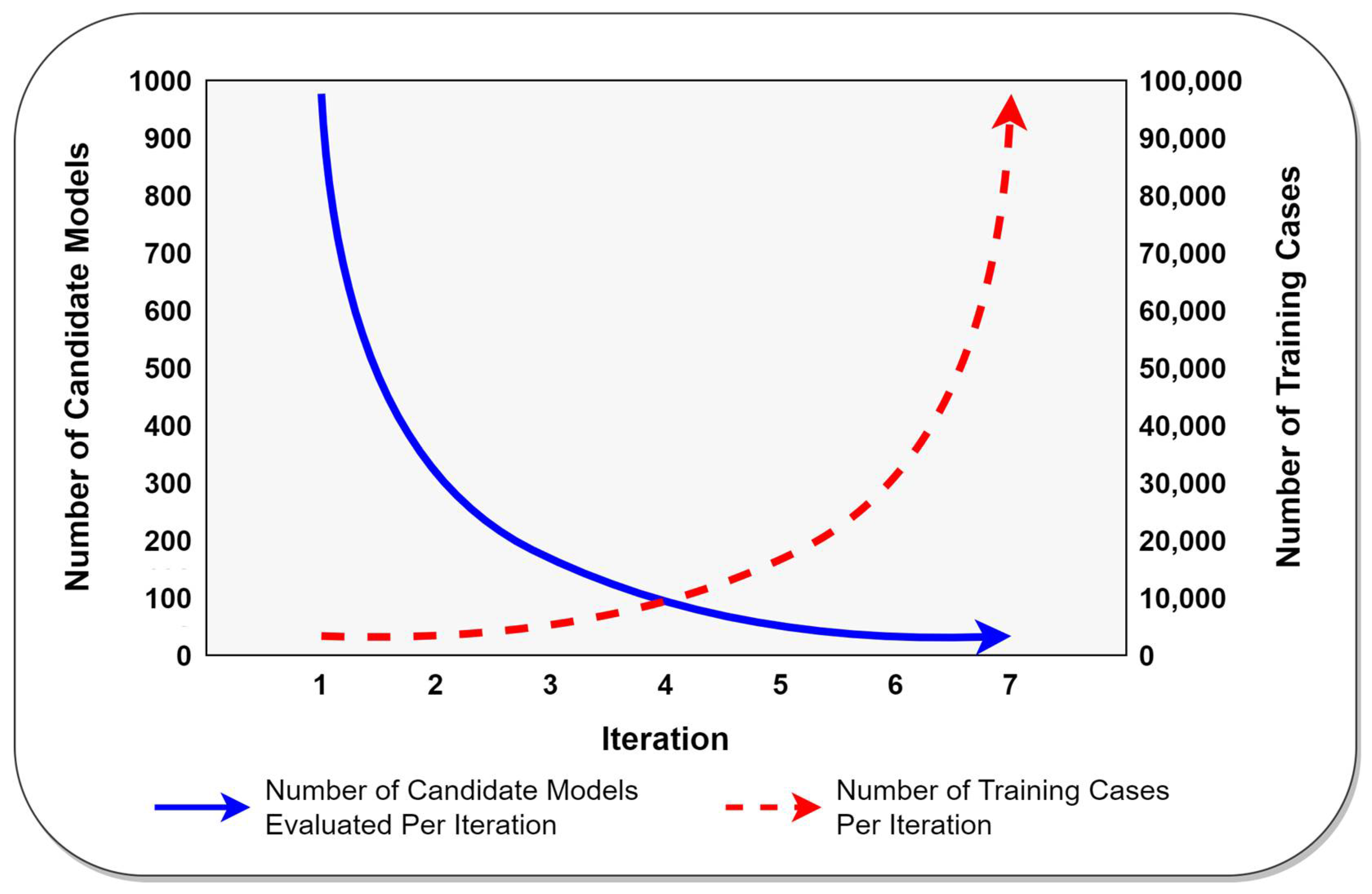
As illustrated in Figure 2, both the number of candidate ML models and the number of training cases that will be used during each iteration of the successive halving algorithm are determined by exponential functions and can be easily calculated before the algorithm begins evaluating any ML models. Since the number of models needed for each successive halving iteration can be easily calculated in advance, the current successive halving iteration can be terminated immediately as soon as the number of ML models needed for the next iteration have been fully evaluated via greedy cross validation. Put differently, there is no need to wait until every candidate model for the current iteration has been fully evaluated before identifying the set of best-performing models that will be used in the next iteration. Instead, by virtue of greedy cross validation’s innate prioritization of the most promising ML models, any iteration of successive halving (except the final iteration) can be concluded immediately as soon as greedy cross validation has fully evaluated a sufficient number of models to satisfy the input requirements of the next iteration. This is the key insight that endows greedy successive halving with its superior performance.

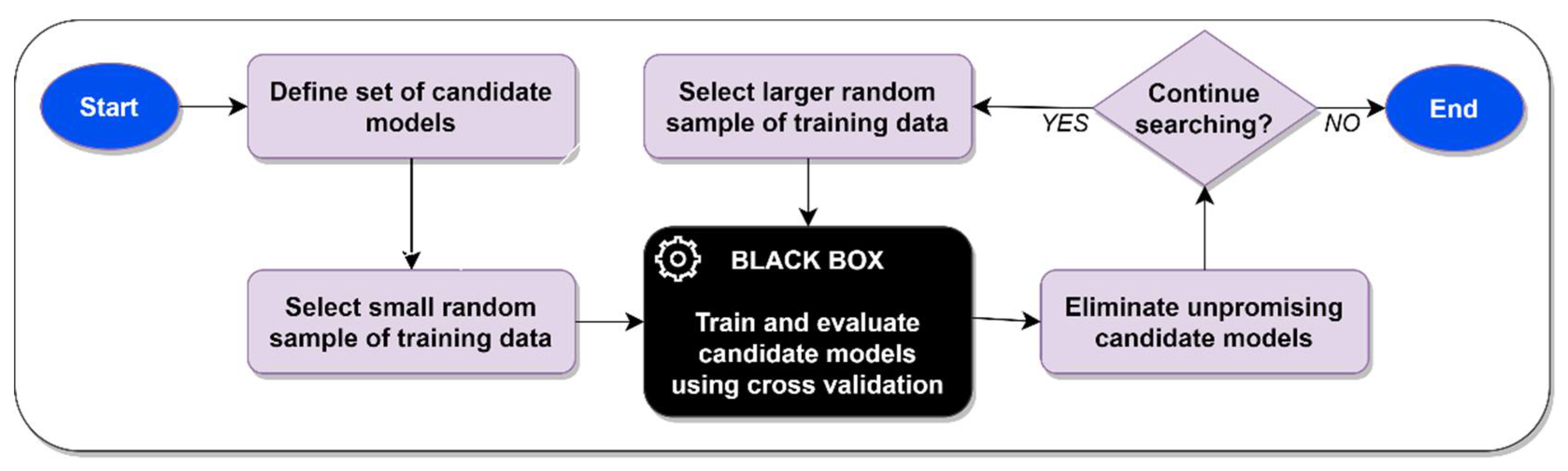
Successive halving—including greedy successive halving—is an iterative algorithm. During the first iteration, successive halving considers the complete set of candidate ML models but does so using a minimally sized random sample of the available training data. By the time successive halving reaches the final iteration, it considers only the two most promising candidate models but does so using all of the available training data. For the current study, the maximum number of training cases to use per iteration ($N_{max}$) was thus set equal to the total number of available training cases, while the minimum number of training cases to use per iteration ($N_{min}$) was set equal to $6\ast k$, with $k$ being the number of folds to use during the cross-validation process. Since 5 and 10 are the two most common values of $k$ used by AI/ML practitioners [17], setting $N_{min}=6\ast k$ guaranteed that a minimum of $6\ast 5=30$ cases would be used to train and evaluate each candidate model during the first iteration of the successive halving algorithm.

In successive halving, the amount by which the number of candidate models is reduced from one iteration to the next and the amount by which the number of training cases is increased from one iteration to the next both depend on exponential functions, which in turn depend on the number of successive halving iterations. Prior to calculating the parameters of the exponential functions, it is therefore necessary to calculate the number of iterations that will be needed during the successive halving process. The total number of iterations to perform ($N_{iter}$) is a function of the minimum and maximum number of cases per iteration and a halving factor ($h$), as shown in Equation (1). Each successive halving iteration considers approximately $1/h$ of the models from the previous iteration. For the current study, the halving factor was set equal to 3, which matches the default value used in scikit-learn’s implementation of the successive halving algorithm [15].

$$N_{iter}=\lfloor {\log }_h\left(N_{max} / N_{min}\right)\rfloor +1$$

(1)

Once the number of successive halving iterations is known, the number of ML models to use and the number of training cases to use for any iteration can be easily calculated using exponential functions of the form $y=a·e^{x·b}$. Specifically, for any iteration $i$ (where $i=0$ for the first iteration), the number of ML models that are needed for the next iteration ($N_{models}$) can be determined by Equation (2), while the number of training cases to use for the current iteration ($N_{cases}$) can be determined by Equation (3).

$$\begin{array}{c}{N}_{models}=n\left(M\right)\ast e^{-\left(i+1\right)·b_{models}}\\ \mathrm{where}:\\ M=\mathrm{the}\mathrm{set}\mathrm{of}\mathrm{candidate}\mathrm{models}\\ n\left(M\right)=\mathrm{the}\mathrm{cardinality}\mathrm{of} M\\ b_{models}=\frac{\ln \left(2 / n\left(M\right)\right)}{-N_{iter}+1}\end{array}$$

(2)

$$\begin{array}{c}{N}_{cases}=N_{min}\ast e^{i·b_{cases}}\\ \mathrm{where}:\\ b_{cases}=\frac{\ln \left(N_{max} / N_{min}\right)}{N_{iter}-1}\end{array}$$

(3)

As soon as the number of training cases to use for the current iteration ($N_{cases}$) is known (per Equation (3)), a random sample of $N_{cases}$ training cases can be drawn from the complete set of training data, which can then be randomly subdivided into k folds. Next, Equation (2) can be used to calculate the number of candidate ML models ($N_{models}$) that will be needed as input for the next iteration. If the current iteration also happens to be the algorithm’s final iteration, then $N_{models}$ will naturally be equal to 1, indicating that the single, best-performing model is to be returned. Once the value of $N_{models}$ is known, the evaluation of the candidate models for the current iteration can begin.

It is at this point that the greedy successive halving algorithm diverges from the standard successive halving algorithm. With standard successive halving, the next step would be to completely evaluate the performance of every remaining candidate ML model by using standard cross validation. After the overall performance of every remaining candidate ML model has been identified, the standard successive halving algorithm would select the $N_{models}$ best-performing models, which would subsequently be advanced to the next iteration [11]. Any models that did not perform sufficiently well to survive to the next iteration would be discarded. Note that with standard successive halving, every remaining candidate model must be fully evaluated before the algorithm can proceed to the next iteration.

In contrast to standard successive halving, the greedy successive halving algorithm does not require every remaining candidate ML model to be fully evaluated before it is able to proceed to the next iteration. Instead, greedy successive halving is able to advance to the next iteration as soon as it has fully evaluated just $N_{models}$ of the remaining candidate models. This key advantage is attributable to greedy successive halving’s use of greedy cross validation, which automatically prioritizes the evaluation of the most promising ML models. A complete description of the proposed greedy successive halving algorithm is provided in Algorithm 1 below.

Algorithm 1. ML model selection using greedy successive halving.

Input:  M (set of candidate ML models), k (number of folds), D (training dataset),

h (halving factor)

Output: Best-performing ML model identified in M

$N_{max}\leftarrow n\left(D\right) \left(\mathrm{maximum}\#\mathrm{of}\mathrm{training}\mathrm{cases}\mathrm{to}\mathrm{use}\mathrm{per}\mathrm{iteration}\right)$

$N_{min}\leftarrow 6k \left(\mathrm{minimum}\#\mathrm{of}\mathrm{training}\mathrm{cases}\mathrm{to}\mathrm{use}\mathrm{per}\mathrm{iteration}\right)$

$N_{iter}\leftarrow \lfloor {\log }_h\left(N_{max} / N_{min}\right)\rfloor +1 \left(\mathrm{total}\#\mathrm{of}\mathrm{halving}\mathrm{iterations}\mathrm{to}\mathrm{perform}\right)$

$b_{cases}\leftarrow \frac{\ln \left(N_{max} / N_{min}\right)}{N_{iter}-1}\left(\mathrm{scalar}\mathrm{for}\mathrm{computing}\#\mathrm{of}\mathrm{training}\mathrm{cases}\mathrm{to}\mathrm{use}\mathrm{per}\mathrm{iteration}\right)$

$b_{models}\leftarrow \frac{\ln \left(2 / n\left(M\right)\right)}{-N_{iter}+1}\left(\mathrm{scalar}\mathrm{for}\mathrm{computing}\#\mathrm{of}\mathrm{best}\mathrm{models}\mathrm{to}\mathrm{select}\mathrm{per}\mathrm{iteration}\right)$

$for each i\in \left\{0,1,\dots ,N_{iter}-1\right\} \mathbf{do}$ (for each halving iteration)

$M_{best}=\varnothing \left(\mathrm{the}\mathrm{set}\mathrm{of}\mathrm{best}\mathrm{models}\mathrm{selected}\mathrm{during}\mathrm{this}\mathrm{iteration}\right)$

$(\mathrm{determine}\mathrm{the}\#\mathrm{of}\mathrm{best}\mathrm{models}\mathrm{to}\mathrm{retain}\mathrm{after}\mathrm{this}\mathrm{iteration})$:

$if i=N_{iter}-1then$

$N_{models}\leftarrow 1$

$else$

$N_{models}\leftarrow \min \left(n\left(M\right),\mathrm{round}\left(n\left(M\right)\ast e^{-\left(i+1\right)·b_{models}}\right)\right)$

$endif$

$N_{cases}\leftarrow \mathrm{round}\left(N_{min}\ast e^{i·b_{cases}}\right) \left(\#\mathrm{of}\mathrm{training}\mathrm{cases}\mathrm{to}\mathrm{use}\mathrm{during}\mathrm{this}\mathrm{iteration}\right)$

$D^{\ast }\leftarrow \mathrm{random}\mathrm{sample}\mathrm{of}{N}_{cases}\mathrm{training}\mathrm{cases}\mathrm{selected}\mathrm{from}D$

$\mathrm{split}{D}^{\ast }\mathrm{into}k\mathrm{folds}\mathrm{of}\mathrm{approximately}\mathrm{equal}\mathrm{size},\mathrm{s}.\mathrm{t}.D^{\ast }=\left\{d_1,d_2,\dots ,d_k\right\}$

$for each m\in M \mathbf{do}$ (for each remaining candidate model)

$\mathrm{train} m \mathrm{using}\mathrm{folds} \left\{d_2,\dots ,d_k\right\}$

$P_m\leftarrow \mathrm{performance}\mathrm{of}m\mathrm{evaluated}\mathrm{using}\mathrm{fold}{d}_1$

$N_m\leftarrow 1\left(\mathrm{number}\mathrm{of}\mathrm{folds}\mathrm{evaluated}\mathrm{for}m\right)$

$while n\left(M_{best}\right)<N_{models} \mathbf{do}\left(\mathrm{while}\mathrm{more}\mathrm{best}\mathrm{models}\mathrm{remain}\mathrm{to}\mathrm{be}\mathrm{selected}\right)$

$m^{\ast }\leftarrow \mathrm{best}\mathrm{incompletely}\mathrm{evaluated}m\in M,\mathrm{per}P$

$N_{m^{\ast }}\leftarrow N_{m^{\ast }}+1$

$\mathrm{train} m^{\ast } \mathrm{using}\mathrm{all}\mathrm{folds} d_j\in D^{\ast } \mathrm{where} j \ne N_{m^{\ast }}$

$\mathrm{evaluate}\mathrm{performance}\mathrm{of} m^{\ast } \mathrm{using}\mathrm{fold} d_{N_{m^{\ast }}}$

$P_{m^{\ast }}\leftarrow \mathrm{mean}\mathrm{performance}\mathrm{of}{m}^{\ast }\mathrm{for}\mathrm{folds} \left\{d_1,\dots ,d_{N_{m^{\ast }}}\right\}$

$\left(\mathrm{if}\mathrm{all}\mathrm{folds}\mathrm{have}\mathrm{been}\mathrm{evaluated}\mathrm{for} m^{\ast },\mathrm{then}\mathrm{add}{m}^{\ast }\mathrm{to}\mathrm{the}\mathrm{set}\mathrm{of}\mathrm{best}\mathrm{models}\right)$:

$if N_{m^{\ast }}=k \mathbf{then}$

$M_{best}\leftarrow m^{\ast }$

$endif$

$endwhile$

$M\leftarrow M_{best} \left(\mathrm{define}\mathrm{the}\mathrm{set}\mathrm{of}\mathrm{remaining}\mathrm{candidate}\mathrm{models}\right)$

$endfor$

$return\mathrm{the}\mathrm{only}\mathrm{remaining}m\in M$

2.2. Evaluative Experiments

Having presented and discussed the proposed greedy successive halving algorithm, it is now possible to describe the extensive series of experiments that were conducted in order to assess, quantify, and compare the performance of greedy successive halving against that of standard successive halving. In total, 60 experiments were carried out to rigorously evaluate the performance characteristics of the proposed greedy successive halving algorithm under a variety of different conditions. These experiments involved five different machine learning algorithms, three of which were classifiers (a Bernoulli naïve Bayes classifier, a decision tree classifier, and a deep neural network classifier) and two of which were regressors (a passive aggressive regressor and a Tweedie regressor). The versions of these algorithms found in Python’s scikit-learn library were used in the experiments to ensure replicability. These specific ML algorithms were chosen because of their widely varying approaches to machine learning [18,19,20,21] and to provide insights into the performance of greedy successive halving in scenarios involving both classification and regression tasks. Four different real-world datasets were used in conjunction with these ML algorithms, with the Wine Recognition dataset [22] and Wisconsin Diagnostic Breast Cancer dataset [23] serving as input for the classification algorithms and the California Housing dataset [24] and Diabetes dataset [25] serving as input for the regression algorithms. These datasets are all well-known among AI/ML practitioners and are freely available in the Python scikit-learn library, thus ensuring that the results of the experiments could be easily replicated. The characteristics of each of these datasets are provided in

Table 1. Characteristics of datasets used in the evaluative experiments.

Dataset	Instances	Features	Target
California Housing	20,640	8	Real
Diabetes	442	10	Real
Wine Recognition	178	13	Three Classes
Wisconsin Diagnostic Breast Cancer	569	29	Two Classes

below.

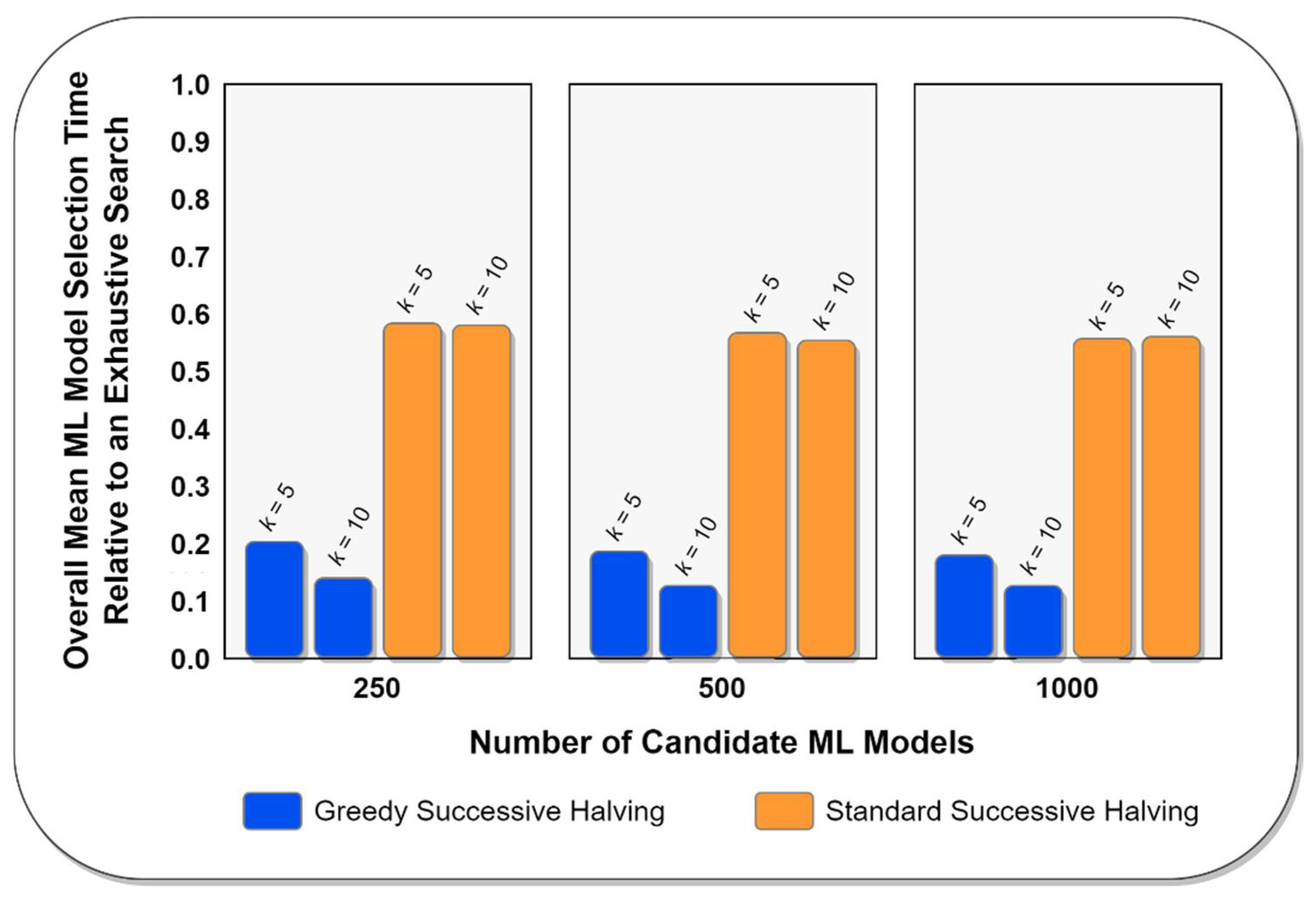
Two possible values for the number of cross-validation folds ($k$) were used in the experiments, with $k\in \left\{5, 10\right\}$. These values of $k$ were adopted because they are the most widely used among AI/ML practitioners when performing cross validation [17]. Additionally, three different values for the number of candidate ML models ($n\left(M\right)$) were also used in the experiments, with $n\left(M\right)\in \left\{250, 500, 1000\right\}$. The set of candidate ML models was randomly generated for each experiment, with care being taken to ensure that each model’s hyperparameter settings were unique within the set. For the models involving deep neural networks, both the algorithmic hyperparameters and the structure of the neural networks (number of hidden layers, number of nodes per layer, etc.) were allowed to vary from model to model. In summary, then, 12 different experimental conditions were used for each ML algorithm, yielding an overall total of 60 unique experimental conditions (5 ML algorithms * 2 datasets per algorithm * 2 values of $k$ * 3 different sizes for $M$ = 60 total experiments). Each of these experiments was repeated 30 times in order to ensure that the distributions of the resulting performance metrics would be approximately Gaussian, per the Central Limit Theorem [26].

As noted above, the overall goal of the experiments was to compare the performance of the proposed greedy successive halving algorithm against that of the standard successive halving algorithm under a wide variety of different conditions. With this goal in mind, two different performance metrics were generated for each experiment: (1) the wall-clock time required by each algorithm to choose a final ML model from among the set of candidate models, and (2) the quality of the final model chosen by each algorithm. The first of these performance metrics allowed for an assessment of how quickly the competing algorithms completed the ML model selection task, while the second of these performance metrics allowed the quality of the final model chosen by the greedy successive algorithm to be compared against the quality of the final model chosen by the standard successive halving algorithm. If the greedy successive halving algorithm could be shown to select ML models of statistically comparable quality to those selected by the standard successive halving algorithm while requiring less wall-clock time to do so, then it could be reasonably concluded that the greedy successive halving algorithm is superior to the standard successive halving algorithm.

Among the classifiers, the performance of the final ML model chosen by each of the competing successive halving algorithms was measured in terms of classification accuracy, while among the regressors, the performance of the final model chosen by the competing successive halving algorithms was measured in terms of the mean absolute error (MAE) of the model’s predictions. For each experiment, a naïve, exhaustive search of all of the experiment’s candidate models was first performed using standard k-fold cross validation without successive halving. Since an exhaustive search evaluates every possible candidate model using the complete set of training data for a given experiment, the results of the exhaustive search established a baseline wall-clock processing time for each experiment, as well as a baseline performance value for the ground truth optimal model among the set of candidate models considered during the experiment. The mean performance values for the ground truth optimal models identified during the experiments are provided in

Table 2. Mean performance of ground truth optimal models for each experimental condition, as identified by an exhaustive search.

Dataset	ML Algorithm	250 Candidate Models		500 Candidate Models		1000 Candidate Models
		k = 5	k = 10	k = 5	k = 10	k = 5	k = 10
California Housing †	Passive Aggressive	0.573	0.570	0.555	0.558	0.548	0.548
	Tweedie	0.588	0.584	0.574	0.571	0.571	0.568
Diabetes †	Passive Aggressive	44.482	44.345	44.380	44.253	44.320	44.218
	Tweedie	44.016	43.982	43.988	43.954	43.978	43.940
Wine Recognition ‡	Bernoulli Naïve Bayes	0.914	0.920	0.917	0.923	0.918	0.924
	Decision Tree	0.923	0.935	0.929	0.939	0.934	0.946
	Deep Neural Network	0.979	0.983	0.980	0.985	0.982	0.986
Wisconsin Diagnostic Breast Cancer ‡	Bernoulli Naïve Bayes	0.940	0.940	0.940	0.942	0.941	0.942
	Decision Tree	0.953	0.955	0.955	0.958	0.957	0.958
	Deep Neural Network	0.982	0.982	0.983	0.983	0.984	0.983

^† Values indicate the average MAE for the corresponding experiments’ ground truth optimal models. ^‡ Values indicate the average classification accuracy for the corresponding experiments’ ground truth optimal models.

below. Note that the values reported for the California Housing and Diabetes datasets indicate the average MAE for the corresponding experiments’ ground truth optimal models, while the values reported for the Wine Recognition and Wisconsin Diagnostic Breast Cancer datasets indicate the average classification accuracy for the corresponding experiments’ ground truth optimal models. To better contextualize the MAE values reported in the table, it is also worthwhile to note that the raw values for the target variable in the California Housing dataset ranged from 0.15 to 5.0, while the raw values for the target variable in the Diabetes dataset ranged from 25 to 346.

After all of the experiments were complete, both the performance of the final models chosen by each variant of the successive halving algorithm and the wall-clock time required by each variant were standardized as percentages of their corresponding baseline values. For example, a standardized performance value of 1.02 for a regressor model would indicate that the mean absolute error for the chosen model was 2% greater than the ground truth optimal model, while a standardized performance value of 0.98 for a classifier model would indicate that the classification accuracy of the chosen model was 2% less than the ground truth optimal model. Similarly, a standardized time of 0.30 would indicate that a successive halving algorithm required only 30% as much wall-clock time as a corresponding exhaustive search of the same set of candidate models. Using this approach allowed the performance of the competing algorithms to be compared across experimental conditions in a statistically valid way. Finally, the standardized wall-clock times and model performance values for the standard and greedy successive halving algorithms were compared against each other using Welch’s t-tests [27]. Unlike most other t-tests, Welch’s t-tests allow the independent samples being compared to have unequal variances. Since there was no ex ante reason to expect the distributional variances of the performance metrics generated by each competing algorithm to be equal, Welch’s t-tests provided an appropriate statistical foundation for comparing the experimental results.

The experiments themselves were run sequentially using a fixed hardware configuration on the Google Cloud Platform [28]. Since the hardware resources used to conduct the experiments were identical for each experimental condition, any statistically significant differences in wall-clock times or model performance values would be attributable solely to differences between the standard successive halving algorithm and the greedy successive halving algorithm. The results of the experiments are presented in the following section.

3. Results

As described in the previous section, the experiments carried out in this study were designed to compare the performance of the proposed greedy successive halving algorithm against that of the standard successive halving algorithm under a variety of different conditions. Comparing these algorithms required the consideration of two distinct performance metrics for each of the study’s 60 different experimental conditions: (1) the wall-clock time required by each algorithm to choose a final ML model from among the set of candidate models, and (2) the quality of the final model chosen by each algorithm. If the results of the experiments showed that the greedy successive halving algorithm could select ML models of the same quality as those selected by the standard successive halving algorithm while requiring less wall-clock time to do so, then it would be reasonable to conclude that the greedy successive halving algorithm is generally superior to the standard successive halving algorithm. Accordingly, the performance of the competing algorithms in terms of both wall-clock time and the quality of the chosen ML models is presented in the following subsections.

3.1. Experiment Results: Wall-Clock Time

A necessary first step in comparing the performance of greedy successive halving versus that of standard successive halving was to assess how quickly the competing algorithms were able to complete the task of selecting a final ML model from among a set of candidate models.

Table 3. Mean standardized wall-clock times for evaluation of 250 candidate models, relative to an exhaustive search.

Dataset	ML Algorithm	Greedy Successive Halving		Standard Successive Halving
		k = 5	k = 10	k = 5	k = 10
California Housing	Passive Aggressive	0.041 ***	0.041 ***	0.069	0.077
	Tweedie	0.112 ***	0.093 ***	0.182	0.167
Diabetes	Passive Aggressive	0.242 ***	0.128 ***	0.678	0.640
	Tweedie	0.341 ***	0.156 ***	1.056	0.893
Wine Recognition	Bernoulli Naïve Bayes	0.260 ***	0.187 ***	0.957	0.972
	Decision Tree	0.251 ***	0.166 ***	0.839	0.857
	Deep Neural Network	0.120 ***	0.103 ***	0.470	0.551
Wisconsin Diagnostic Breast Cancer	Bernoulli Naïve Bayes	0.359 ***	0.284 ***	0.891	0.925
	Decision Tree	0.163 ***	0.120 ***	0.389	0.386
	Deep Neural Network	0.102 ***	0.090 ***	0.260	0.292

*** p < 0.001 for a Welch’s t-test comparing wall-clock times for the greedy and standard successive halving algorithms.

,

Table 4. Mean standardized wall-clock times for evaluation of 500 candidate models, relative to an exhaustive search.

Dataset	ML Algorithm	Greedy Successive Halving		Standard Successive Halving
		k = 5	k = 10	k = 5	k = 10
California Housing	Passive Aggressive	0.034 ***	0.034 ***	0.057	0.063
	Tweedie	0.093 ***	0.074 ***	0.157	0.141
Diabetes	Passive Aggressive	0.228 ***	0.121 ***	0.659	0.634
	Tweedie	0.315 ***	0.152 ***	1.028	0.890
Wine Recognition	Bernoulli Naïve Bayes	0.259 ***	0.178 ***	0.971	0.970
	Decision Tree	0.220 ***	0.164 ***	0.821	0.845
	Deep Neural Network	0.111 ***	0.079 ***	0.466	0.473
Wisconsin Diagnostic Breast Cancer	Bernoulli Naïve Bayes	0.335 ***	0.259 ***	0.863	0.892
	Decision Tree	0.149 ***	0.113 ***	0.374	0.372
	Deep Neural Network	0.091 ***	0.063 ***	0.249	0.231

*** p < 0.001 for a Welch’s t-test comparing wall-clock times for the greedy and standard successive halving algorithms.

and

Table 5. Mean standardized wall-clock times for evaluation of 1000 candidate models, relative to an exhaustive search.

Dataset	ML Algorithm	Greedy Successive Halving		Standard Successive Halving
		k = 5	k = 10	k = 5	k = 10
California Housing	Passive Aggressive	0.030 ***	0.030 ***	0.050	0.056
	Tweedie	0.082 ***	0.075 ***	0.142	0.147
Diabetes	Passive Aggressive	0.227 ***	0.130 ***	0.638	0.625
	Tweedie	0.297 ***	0.151 ***	1.004	0.882
Wine Recognition	Bernoulli Naïve Bayes	0.250 ***	0.175 ***	0.953	0.962
	Decision Tree	0.224 ***	0.166 ***	0.834	0.841
	Deep Neural Network	0.106 ***	0.084 ***	0.467	0.551
Wisconsin Diagnostic Breast Cancer	Bernoulli Naïve Bayes	0.322 ***	0.250 ***	0.852	0.874
	Decision Tree	0.145 ***	0.107 ***	0.357	0.354
	Deep Neural Network	0.082 ***	0.068 ***	0.241	0.272

*** p < 0.001 for a Welch’s t-test comparing wall-clock times for the greedy and standard successive halving algorithms.

below summarize the average wall-clock time required by each algorithm to complete the ML model selection task for sets of 250, 500, and 1000 candidate models, respectively. As noted in Section 2, each value reported in these tables has been standardized as a proportion of the corresponding wall-clock time required to complete a naïve, exhaustive search, and reflects the mean of 30 different trials for the specified experimental condition. The probability values reported in the tables originate from Welch’s t-tests that directly compare the standardized wall-clock times required by the competing algorithms under identical experimental conditions.

As shown above in Table 3, Table 4 and Table 5, the greedy successive halving algorithm was consistently able to complete the ML model selection task much more quickly than the standard successive algorithm, regardless of the dataset that was used in the experiment, the type of machine learning algorithm, the number of candidate models being evaluated, or the number of folds used for cross validation. Put differently, the results reported in Table 3, Table 4 and Table 5 indicate that greedy successive halving required less wall-clock time to complete the ML model selection task than standard success halving in all 60 of the experimental conditions considered in this study, with the superior performance of greedy successive halving being statistically significant at the p < 0.001 level in every case. The evidence obtained from the experiments thus strongly suggests that greedy successive halving will be significantly faster than standard successive halving when performing hyperparameter optimization under otherwise identical conditions. The comparative overall average wall-clock times required by the competing successive halving algorithms to complete the ML model selection task for varying numbers of candidate models and folds is illustrated in Figure 6 below.

3.2. Experiment Results: Quality of Chosen Models

Although assessing how quickly the competing algorithms were able to complete the hyperparameter optimization process was necessary, doing so was not by itself sufficient to establish the superiority of the greedy successive halving algorithm. Instead, it was also necessary to compare the quality of the final ML models chosen by the greedy successive algorithm under varying experimental conditions against the quality of the final models chosen by the standard successive halving algorithm under identical conditions. Only if greedy successive halving could be shown to select final ML models of equivalent quality to those selected by standard successive halving—while also being faster to select those models—could it be reasonably concluded that the greedy successive halving algorithm was generally superior to the standard successive halving algorithm. Accordingly, Table 4, Table 5 and

Table 6. Mean standardized quality of final ML models chosen from a set of 250 candidate models, relative to ground truth optimal model.

Dataset	ML Algorithm	Greedy Successive Halving		Standard Successive Halving
		k = 5	k = 10	k = 5	k = 10
California Housing	Passive Aggressive	1.021	1.031	1.010	1.007
	Tweedie	1.012	1.013	1.002	1.000
Diabetes	Passive Aggressive	1.034	1.097	1.029	1.039
	Tweedie	1.054	1.040	1.028	1.027
Wine Recognition	Bernoulli Naïve Bayes	0.968	0.979	0.974	0.984
	Decision Tree	0.908	0.944	0.903	0.939
	Deep Neural Network	0.963	0.987	0.974	0.985
Wisconsin Diagnostic Breast Cancer	Bernoulli Naïve Bayes	0.993	0.993	0.993	0.994
	Decision Tree	0.979	0.978	0.983	0.979
	Deep Neural Network	0.989	0.992	0.989	0.994

below summarize the average quality of the final ML models chosen by the competing successive halving algorithms for sets of 250, 500, and 1000 candidate models, respectively.

As noted in Section 2, each value reported in Table 6,

Table 7. Mean standardized quality of final ML models chosen from a set of 500 candidate models, relative to ground truth optimal model.

Dataset	ML Algorithm	Greedy Successive Halving		Standard Successive Halving
		k = 5	k = 10	k = 5	k = 10
California Housing	Passive Aggressive	1.023	1.016	1.010	1.008
	Tweedie	1.020	1.018	1.004	1.002
Diabetes	Passive Aggressive	1.049	1.068	1.030	1.039
	Tweedie	1.054	1.035	1.031	1.025
Wine Recognition	Bernoulli Naïve Bayes	0.961	0.971	0.974	0.977
	Decision Tree	0.912	0.936	0.926	0.936
	Deep Neural Network	0.968	0.983	0.973	0.983
Wisconsin Diagnostic Breast Cancer	Bernoulli Naïve Bayes	0.992	0.992	0.994	0.993
	Decision Tree	0.974	0.975	0.974	0.977
	Deep Neural Network	0.989	0.991	0.988	0.993

and

Table 8. Mean standardized quality of final ML models chosen from a set of 1000 candidate models, relative to ground truth optimal model.

Dataset	ML Algorithm	Greedy Successive Halving		Standard Successive Halving
		k = 5	k = 10	k = 5	k = 10
California Housing	Passive Aggressive	1.021	1.017	1.020	1.007
	Tweedie	1.025	1.010	1.008	1.002
Diabetes	Passive Aggressive	1.050	1.099	1.031	1.042
	Tweedie	1.054	1.038	1.030	1.026
Wine Recognition	Bernoulli Naïve Bayes	0.961	0.968	0.974	0.976
	Decision Tree	0.879	0.915	0.903	0.925
	Deep Neural Network	0.968	0.983	0.975	0.979
Wisconsin Diagnostic Breast Cancer	Bernoulli Naïve Bayes	0.992	0.991	0.993	0.992
	Decision Tree	0.972	0.972	0.974	0.977 **
	Deep Neural Network	0.986	0.990	0.988	0.992

** p < 0.01, for a Welch’s t-test comparing the quality of the final ML models chosen by the greedy and standard successive halving algorithms.

has been standardized relative to the quality of the ground truth optimal model for each experimental condition, as identified by means of an exhaustive search. For experiments involving a classification task (i.e., those experiments that relied on the Bernoulli naïve Bayes, decision tree, or deep neural network classifiers), the values in the tables represent the average classification accuracy of the final ML models chosen by each algorithm, relative to the classification accuracy of the ground truth optimal model within the corresponding set of candidate models. For experiments involving a regression task (i.e., those experiments that relied on the passive aggressive or Tweedie regressors), the values in the tables represent the average mean absolute error (MAE) of the final ML models chosen by each algorithm, relative to the MAE of the ground truth optimal model within the corresponding set of candidate models. As with the wall-clock times presented earlier in this section, the values reported in the tables below reflect the mean of 30 different trials for each experimental condition, with the corresponding probability values originating from Welch’s t-tests that directly compared the quality of the final ML models chosen by the competing algorithms under identical experimental conditions.

As shown in Table 6, Table 7 and Table 8, the greedy successive halving algorithm chose final ML models whose quality was statistically indistinguishable from the final models chosen by the standard successive algorithm in 59 out of the 60 different experimental conditions considered in the current study. Put differently, the results reported in Table 6, Table 7 and Table 8 indicate that the average quality of the final ML models chosen by the greedy and standard successive halving algorithms is statistically identical approximately 98.3% of the time, regardless of the dataset, the type of machine learning algorithm, the number of candidate models being evaluated, or the number of folds used for cross validation. The only exception to the algorithms’ otherwise statistically identical ML model selection capabilities was the experimental condition in which a decision tree was used in conjunction with 1000 different candidate models and 10 cross-validation folds to classify cases for the Wisconsin Diagnostic Breast Cancer dataset. In this rare exception, the standard successive halving algorithm chose final ML models whose classification accuracy was, on average, 0.5% closer to the classification accuracy of the ground truth optimal model than the final models chosen by the greedy successive halving algorithm, with this difference being statistically significant at the p < 0.01 level. In all other cases, greedy successive halving was observed to perform identically with standard successive halving in terms of its ability to select high-performing ML models.

Finally, it is worth noting that neither the standard successive halving algorithm nor the greedy successive halving algorithm will choose the ground truth optimal model on average. Among the 24 experimental conditions involving regression problems, both the greedy and standard successive halving algorithms were observed to select final ML models whose mean absolute errors were slightly higher on average than the true optimal ML model within the set of available candidate models. Similarly, among the 36 experimental conditions involving classification problems, both the greedy and standard successive halving algorithms were observed to select final ML models whose classification accuracies were slightly lower on average than the true optimal ML model within the set of available candidate models. For both greedy and standard successive halving, then, the choice to use a successive halving algorithm to perform hyperparameter optimization rather than relying on an exhaustive search represents a tradeoff in which substantial gains in search speed are realized in exchange for an outcome that will, on average, be slightly sub-optimal.

4. Discussion

4.1. Summary and Discussion of Findings

The results of the experiments described in the previous section indicate (1) that the greedy successive halving algorithm was significantly faster than the standard successive halving algorithm in 100% of the experimental conditions considered in the study; and (2) that the greedy successive halving algorithm was able to select final ML models whose quality was statistically identical to the models chosen by standard successive halving in approximately 98.3% of those conditions. Since greedy successive halving was observed to always be much faster than standard successive halving, and since greedy successive halving almost always chose final models of the same quality as standard successive halving, it can be reasonably concluded that the proposed greedy successive halving algorithm is generally superior to the standard successive halving algorithm in terms of its ability to perform hyperparameter optimization for AI/ML scenarios.

While the results reported in the previous section provide insights into the comparative performance of greedy successive halving in specific scenarios, some consideration and discussion of the proposed algorithm’s average level of performance in comparison to standard successive halving may be instructive. To this end, across all 60 of the experimental conditions evaluated in the study, greedy successive halving was, on average, 3.59 times faster than standard successive halving when performing identical ML model selection tasks, with greedy successive halving’s advantage in speed ranging from a minimum of 2.65 times faster to a maximum of 5.42 times faster than standard successive halving. This remarkable difference in the speed with which greedy successive halving can complete the hyperparameter optimization process has very significant implications for AI/ML practitioners. For example, given a desire to complete the hyperparameter optimization process as quickly and inexpensively as possible, and assuming the use of identical hardware resources, AI/ML practitioners relying on greedy successive halving would be able to evaluate the same number of candidate ML models 3.59 times more quickly than if they had chosen to use standard successive halving to perform the same task. Conversely, AI/ML researchers working within the constraints of a computational budget could evaluate a much larger set of candidate ML models during a fixed timeframe than would be possible with standard successive halving, thus markedly improving the chances of identifying a superior final model.

4.2. Limitations and Opportunities for Future Research

Although careful and systematic efforts were taken in this study to investigate the performance of the proposed greedy successive halving algorithm in comparison to that of the standard successive halving algorithm, there nevertheless remain several limitations to this work that merit acknowledgement. First, the experiments described herein relied on four different datasets, two of which involved classification problems and two of which involved regression problems. These datasets are heterogeneous in terms of their number of cases and their numbers of independent and dependent variables, and are publicly available and easily accessible to aid in the reproducibility of the study’s findings. Despite these advantages and the observed consistency of the results of the experiments across datasets, it is possible that the greedy successive halving algorithm would perform differently if used with other datasets. Future research should thus subject the greedy successive halving algorithm to other datasets with varying characteristics in order to ascertain the extent to which greedy successive halving performs consistently across a wide variety of datasets.

In addition to relying on just four different datasets, the findings of the experiments reported herein are also limited insofar as they relied on only five different machine learning algorithms. Although care was taken to include three different ML classifier algorithms and two different ML regressors in the study, and although the ML algorithms used in the experiments were chosen because of their widely varying approaches to machine learning, there remain dozens of other ML algorithms that were not included in this investigation. Future research in this area should therefore endeavor to evaluate the performance of greedy successive halving when used as a basis for rapid hyperparameter optimization in AI/ML scenarios involving other popular machine learning algorithms.

Next, the experiments described in the current study evaluated the comparative performance of the greedy successive halving algorithm at selecting a high-performing ML model from sets of 250, 500, and 1000 different candidate models. There is some evidence in the results from the experiments that suggests that the relative speed with which the greedy successive halving algorithm is able to complete the ML model selection task tends to improve in comparison to an exhaustive search as the number of candidate models increases. The nature of the relationship between the cardinality of the set of candidate models and the advantage in speed that the greedy successive halving algorithm has over an exhaustive search was not formally studied in this paper, and this represents another opportunity for future research.

Finally, the standard successive halving algorithm, the proposed greedy successive halving algorithm, and the exhaustive search algorithm against which the competing successive halving algorithms were compared were all implemented in this study as serial processes. Although doing so would not be trivial, it would certainly be feasible to develop versions of the greedy successive halving algorithm that take advantage of parallel processing. It is currently unknown how well the performance of a parallel implementation of the greedy successive halving algorithm would compare against the performance of a parallel implementation of the standard successive halving algorithm. Developing and evaluating the performance of a parallel version of the greedy successive halving algorithm is thus a potentially very fruitful opportunity for future research on state-of-the-art hyperparameter optimization.

4.3. Concluding Remarks

This paper demonstrated that greedy cross validation can be seamlessly integrated into the popular successive halving method to create a greedy successive halving algorithm that can perform very rapid hyperparameter optimization for artificial intelligence and machine learning scenarios. The performance of the proposed greedy successive halving algorithm was rigorously compared against the performance of the standard successive halving algorithm under 60 different experimental conditions, with these experiments involving four different real-world datasets, five different machine learning algorithms (including three distinct classifier algorithms and two distinct regressor algorithms), sets of candidate ML models of three different sizes, and two different values for the number of folds used during the cross-validation process. The results of the experiments showed that on average, the proposed greedy successive halving algorithm is more than 3.59 times faster than the standard successive halving algorithm at completing identical hyperparameter optimization tasks. Furthermore, the results showed that the quality of the final ML models chosen by the greedy successive halving algorithm are statistically identical to the quality of the final ML models chosen by the standard successive halving algorithm approximately 98.3% of the time. Since the proposed greedy successive halving algorithm is much, much faster than the standard successive halving algorithm while almost always being able to select final ML models of equal quality, AI and ML researchers would be well-advised to consider using greedy successive halving rather than standard successive halving when performing hyperparameter optimization.

Despite the overwhelming evidence in favor of the superiority of the greedy successive halving algorithm that emerged from the experiments described in this study, much remains to be learned. For example, the current paper considered the performance of greedy successive halving only in the context of hyperparameter optimization for AI/ML-related use cases. It seems reasonable to expect, however, that greedy successive halving could be readily adapted for use in many other scenarios to which computational optimization techniques may be beneficially applied. Among these alternate uses, one particularly noteworthy area of inquiry would be to recast greedy successive halving for use in solving a variety of different bandit problems or other reinforcement learning problems that involve an exploration/exploitation dilemma. These and many other possibilities have yet to be explored, and, at least for now, remain as tantalizing opportunities for future research.

References

1. Feurer, M.; Hutter, F. Hyperparameter Optimization. In Automated Machine Learning: Methods, Systems, Challenges; Hutter, F., Kotthoff, L., Vanschoren, J., Eds.; Springer: Cham, Switzerland, 2019; pp. 3–33. [Google Scholar]
2. Li, L.; Jamieson, K.; Rostamizadeh, A.; Gonina, E.; Ben-Tzur, J.; Hardt, M.; Recht, B.; Talwalkar, A. A System for Massively Parallel Hyperparameter Tuning. In Proceedings of the 3rd Machine Learning and Systems Conference, Austin, TX, USA, 26–27 November 2020. [Google Scholar]
3. Agrawal, T. Hyperparameter Optimization in Machine Learning: Make Your Machine Learning and Deep Learning Models More Efficient; Apress: New York, NY, USA, 2020. [Google Scholar]
4. Kohavi, R.; John, G.H. Automatic Parameter Selection by Minimizing Estimated Error. In Proceedings of the 12th International Conference on Machine Learning, Tahoe City, CA, USA, 1 February 1995; pp. 304–312. [Google Scholar]
5. Olson, R.S.; Cava, W.L.; Mustahsan, Z.; Varik, A.; Moore, J.H. Data-Driven Advice for Applying Machine Learning to Bioinformatics Problems. In Proceedings of the Pacific Symposium on Biocomputing, Kohala Coast, HI, USA, 4–8 January 2018; pp. 192–203. [Google Scholar]
6. Krizhevsky, A.; Sutskever, I.; Hinton, G.E. ImageNet Classification with Deep Convolutional Neural Networks. Commun. ACM 2017, 60, 84–90. [Google Scholar] [CrossRef] [Green Version]
7. Vanwinckelen, G.; Blockeel, H. Look Before You Leap: Some Insights into Learner Evaluation with Cross-Validation. In Proceedings of the European Conference on Machine Learning and Principles and Practice of Knowledge Discovery in Databases, Workshop on Statistically Sound Data Mining, Nancy, France, 8 December 2014; pp. 3–20. [Google Scholar]
8. Soper, D.S. Greed Is Good: Rapid Hyperparameter Optimization and Model Selection Using Greedy k-Fold Cross Validation. Electronics 2021, 10, 1973. [Google Scholar] [CrossRef]
9. Bengio, Y. Gradient-Based Optimization of Hyperparameters. Neural Comput. 2000, 12, 1889–1900. [Google Scholar] [CrossRef] [PubMed]
10. Franceschi, L.; Donini, M.; Frasconi, P.; Pontil, M. Forward and Reverse Gradient-Based Hyperparameter Optimization. In Proceedings of the 34th International Conference on Machine Learning, Sydney, Australia, 6–11 August 2017; pp. 1165–1173. [Google Scholar]
11. Jamieson, K.; Talwalkar, A. Non-Stochastic Best Arm Identification and Hyperparameter Optimization. In Proceedings of the 8th International Conference on Artificial Intelligence and Statistics, Cadiz, Spain, 22–26 July 2016; pp. 240–248. [Google Scholar]
12. Li, L.; Jamieson, K.; DeSalvo, G.; Rostamizadeh, A.; Talwalkar, A. Hyperband: A Novel Bandit-Based Approach to Hyperparameter Optimization. J. Mach. Learn. Res. 2017, 18, 6765–6816. [Google Scholar]
13. Snoek, J.; Larochelle, H.; Adams, R.P. Practical Bayesian Optimization of Machine Learning Algorithms. Adv. Neural Inf. Process. Syst. 2012, 25, 2951–2959. [Google Scholar]
14. Young, S.R.; Rose, D.C.; Karnowski, T.P.; Lim, S.-H.; Patton, R.M. Optimizing Deep Learning Hyper-Parameters Through an Evolutionary Algorithm. In Proceedings of the Workshop on Machine Learning in High-Performance Computing Environments, Austin, TX, USA, 15 November 2015; pp. 1–5. [Google Scholar]
15. Pedregosa, F.; Varoquaux, G.; Gramfort, A.; Michel, V.; Thirion, B.; Grisel, O.; Blondel, M.; Prettenhofer, P.; Weiss, R.; Dubourg, V. Scikit-Learn: Machine Learning in Python. J. Mach. Learn. Res. 2011, 12, 2825–2830. [Google Scholar]
16. Kumar, R. Machine Learning Quick Reference: Quick and Essential Machine Learning Hacks for Training Smart Data Models; Packt Publishing: Birmingham, UK, 2019. [Google Scholar]
17. Liu, L.; Özsu, M.T. Encyclopedia of Database Systems; Springer: New York, NY, USA, 2009; Volume 6. [Google Scholar]
18. Schütze, H.; Manning, C.D.; Raghavan, P. Introduction to Information Retrieval; Cambridge University Press: Cambridge, UK, 2008; Volume 39. [Google Scholar]
19. Hastie, T.; Tibshirani, R.; Friedman, J.H. The Elements of Statistical Learning: Data Mining, Inference, and Prediction, 2nd ed.; Springer: New York, NY, USA, 2016. [Google Scholar]
20. Crammer, K.; Dekel, O.; Keshet, J.; Shalev-Shwartz, S.; Singer, Y. Online Passive-Aggressive Algorithms. J. Mach. Learn. Res. 2006, 7, 551–585. [Google Scholar]
21. McCullagh, P.; Nelder, J.A. Generalized Linear Models, 2nd ed.; Chapman & Hall: London, UK, 2019. [Google Scholar]
22. Lichman, M. UCI Machine Learning Repository; University of California Irvine, School of Information and Computer Science: Irvine, CA, USA, 2013. [Google Scholar]
23. Mangasarian, O.L.; Street, W.N.; Wolberg, W.H. Breast Cancer Diagnosis and Prognosis via Linear Programming. Oper. Res. 1995, 43, 570–577. [Google Scholar] [CrossRef] [Green Version]
24. Pace, R.K.; Barry, R. Sparse Spatial Autoregressions. Stat. Probab. Lett. 1997, 33, 291–297. [Google Scholar] [CrossRef]
25. Efron, B.; Hastie, T.; Johnstone, I.; Tibshirani, R. Least Angle Regression. Ann. Stat. 2004, 32, 407–499. [Google Scholar] [CrossRef] [Green Version]
26. Wasserman, L. All of Statistics: A Concise Course in Statistical Inference; Springer: New York, NY, USA, 2013. [Google Scholar]
27. Welch, B.L. The Generalization of “Student’s” Problem When Several Different Population Variances are Involved. Biometrika 1947, 34, 28–35. [Google Scholar] [CrossRef] [PubMed]
28. Google. Google Cloud Platform; Alphabet, Inc.: Mountain View, CA, USA, 2022. [Google Scholar]
Figure 1. Generating a candidate machine learning model.
Algorithms 16 00017 g001
Figure 2. A graphical representation of the successive halving algorithm.
Algorithms 16 00017 g002
Figure 3. Standard k-fold cross validation using k = 5 folds.
Algorithms 16 00017 g003
Figure 4. Standard cross validation used as a black-box process in successive halving.
Algorithms 16 00017 g004
Figure 5. An illustrative example of greedy cross validation. Adapted from Soper [8].
Algorithms 16 00017 g005
Figure 6. Comparative mean standardized wall-clock times required to perform hyperparameter optimization, relative to an exhaustive search.
Algorithms 16 00017 g006