Article

On Modeling Antennas Using MoM-Based Algorithms: Wire-Grid versus Surface Triangulation

by
Adnan Alhaj Hasan
,
Aleksey A. Kvasnikov
,
Dmitriy V. Klyukin
,
Anton A. Ivanov
,
Alexander V. Demakov
,
Dmitry M. Mochalov
and
Sergei P. Kuksenko
*
Department of Television and Control, Tomsk State University of Control Systems and Radioelectronics, 634050 Tomsk, Russia
*
Author to whom correspondence should be addressed.
Algorithms 2023, 16(4), 200; https://doi.org/10.3390/a16040200
Submission received: 1 March 2023 / Revised: 24 March 2023 / Accepted: 31 March 2023 / Published: 7 April 2023
(This article belongs to the Special Issue Computational Methods and Optimization for Numerical Analysis)

Abstract

:
This paper focuses on antenna modeling using wire-grid and surface triangulation as two of the most commonly used MoM-based approaches in this field. A comprehensive overview is provided for each of them, including their history, applications, and limitations. The mathematical background of these approaches is briefly presented. Two working algorithms were developed and described in detail, along with their implementations using acceleration techniques. The wire-grid-based algorithm enables modeling of arbitrary antenna solid structures using their equivalent grid of wires according to a specific modeling recommendation proposed in earlier work. On the other hand, the surface triangulation-based algorithm enables calculation of antenna characteristics using a novel excitation source model. Additionally, a new mesh generator based on the combined use of the considered algorithms is developed. These algorithms were used to estimate the characteristics of several antenna types with different levels of complexity. The algorithms computational complexities were also obtained. The results obtained using these algorithms were compared with those obtained using the finite difference time domain numerical method, as well as those calculated analytically and measured. The analysis and comparisons were performed on the example of a rectangle spiral, a spiral, rounded bow-tie planar antennas, biconical, and horn antennas. Furthermore, the validity of the proposed algorithms is verified using the Monte Carlo methodology.

1. Introduction

Full-wave analysis based on numerical methods is widely used to design antenna arrays and elements. For example, antennas can be analyzed using the finite-difference time-domain method (FDTD) [1,2], the finite integration technique [3,4], or the finite element method (FEM) [5,6]. Using such methods and others, numerous approaches were proposed to model and discretize general structures [7,8]. However, the most common method for antenna modeling is the method of moments (MoM) [9,10,11,12]. The popularity of the MoM is probably associated with its relatively low computational costs, which are ensured by the need to discretize only the surfaces of the modeled object, rather than the entire solution domain.
In the process of antenna modeling by the MoM, usually the conductive structures are replaced by equivalent surface currents, and then, using the reciprocity principle, the radiation problem is solved on the basis of these currents. The most important parts of this process are the discretization of the antenna model and the approximation of surface currents within each discrete section, which are usually performed using two basic algorithms: wire-grid and surface triangulation. In the first widely used algorithm, the conductive surfaces of the antenna are replaced by a grid of thin wires with a radius much smaller than the wavelength of the excitation signal and the length of the wires themselves [13,14,15]. This approach enables using a scalar current density function instead of a vector one, which reduces the computational cost of modeling. At the same time, the wire-grid algorithm is relatively poor suited for approximating complex and highly detailed antenna structures and for near-field problems [16]. In the second one, the conductive antenna elements are discretized by triangular surface patches and the vector Rao-Wilton-Glisson (RWG) basis functions are used to approximate the currents [17,18,19]. Triangles describe curvilinear surfaces with a high accuracy, allowing one to achieve accurate results of the antenna analysis. However, the triangulation process and vector basis functions significantly increase the computational costs.
Without losing the generality, rectangular plates share with wire-grid the same problem of the inability to model a general structure, but they differ in that the former uses surface current densities, while the later uses a fine mesh or grid of crossing wires [20]. Many efforts were paid to develop a technique for modeling nonrectangular plates, since the earlier studies in surface patch modeling were limited only to rectangular ones. Some researchers proposed to expand currents on the problem model as an interconnection of polygonal plates in terms of nonrectangular surface patch modes [21]. While the others decided to deal with the whole problem model at once as a general curved surface, and the nonrectangular surface patches make up a piecewise flat approximation to the surface current density on the surface, which seems to be more general but a slightly more complicated in implementation [22,23]. The researchers investigated their proposed approaches using polygonal plates of different shapes (square, triangle, octagonal, quadrilateral, and other plate shapes), but among all the nonrectangular patches, triangular patches seem to be more universal in structure description and easier to implement. The researchers noticed that the testing results are still reasonable even in cases where some of the quadrilaterals degenerate to triangles [21,24]. Therefore, Gilsson and Rao concentrated their work, which in fact started even earlier than 1978, on using triangular patches [25].
Based on the above, new software codes were developed not only on the wire-grid base, like in the numerical electromagnetic code (NEC) [26], MMANA-GAL [27], CONCEPT-II [28], GEMACS [29], and in AN-SOF [30], but also on the patch surface base like in NEC [31], and in the electromagnetic surface patch code (ESP) [32], and others. Thus, the question of which approach or software to use became important and unneglectable due to the rush developments of the used methods and approaches used, as well as the software based on them by virtue of a linear increase in advances in computer systems. The researchers tried to investigate the efficiency of each approach and describe their limitations, applications, and in some works even recommendations. For example, in [33,34], the authors provided an analytical comparison of wire/surface modeling, while in [35,36,37,38], the authors decided to discuss the differences numerically. But to the best of our knowledge, there is no general work which provides comprehensive overview on the history of each approach, its applications, limitations, and working algorithms. Nor is there any work with analytical and numerical comparisons of their efficiency using own advanced and accelerated implementations on the example of different antenna types, as well as a mesh generator based on their hybridization. The aim of the article is to compare these two MoM-based algorithms and analyze their capabilities in modeling different types of antennas.
The rest of this article is organized as follows. Section 2 describes two algorithms under study and the features of their software implementation. Section 3 presents the results of analyzing several antennas using these algorithms. Section 4 discusses the obtained results and formulates several practical recommendations for antenna modeling. Section 5 provides the conclusions.

2. Materials and Methods

This section presents a general mathematical formulation of the MoM solution of the integral equations. Then, the wire- and triangle-grid surface modeling approaches are overviewed. Based on them, two algorithms are developed and described together with their mathematical background and the codes (Wire-Grid and Triangle-Grid) built on their base. It is noteworthy that the general mathematical background of these approaches is covered and detailed in several literatures, for example in [10,39]. In this paper, only the formulation required for the implementation of the algorithms are described.

2.1. General Mathematical Formulation

Analysis of antenna characteristics based on MoM is carried out by reducing the surface integral equations to system of linear algebraic equations (SLAE). Thus, when an electromagnetic wave incident on a conducting surface, surface electric currents are induced on it, creating a scattered electromagnetic field. Considering that Maxwell’s equations are linear, the total Etot and Htot fields can be represented as a superposition of incident (Einc, Hinc) and scattered (Escat, Hscat) waves. Under the boundary conditions on the surface S of a perfect electric conductor (PEC), the total tangential components of the electric and magnetic fields are described by the expressions
n × Etot(r)|S = n × (Einc(r) + Escat(r))|S = 0,
n × Htot(r)|S = n × (Hinc(r) + Hscat(r))|S = J(r),
where n is the vector of the external normal from the observation point r.
Here, the decomposition into the components of the external incident (Einc, Hinc) and scattered (Escat, Hscat) fields is used. The first two are the components that exist in the absence of the object under consideration, and the latter are the components generated by the induced current J(r) on the surface of this object.
Since the induced magnetic currents M(r) on the surface of perfect electric conductors are zero, the scattered electric and magnetic fields can be expressed through the electric vector A(r) and scalar Φ(r) potentials as
E scat ( r ) = j ω A ( r ) Φ ( r ) ,
H scat ( r ) = 1 μ × A ( r ) .
The Green’s function of free space (homogeneous isotropic medium) G(r, r′), which determines the potential at point r generated by a unit point charge at source point r′, is used to later calculate the vector and scalar potentials [40]
G r , r = e j k r r 4 π r r ,
where k is the wave number.
The vector and scalar potentials can be calculated using the Green’s function G(r, r′), which contains information about the medium in which the electric currents are defined as
A ( r ) = μ S G r , r J r d S ,
Φ ( r ) = 1 j ω ε S G r , r J r d S .
Substituting Equations (5) and (6) into (2) and (3), we obtain
E scat r = j ω μ S G r , r J r d S 1 j ω ε S G r , r J r d S ,
H scat r = S G r , r × J r d S .
Further substitution of (7) into (1) leads to the Electric Field Integral Equation (EFIE)
1 j ω z 0 n × E inc r = n × S G r , r J r + 1 k 2 J r d S ,
where z0 is the free space characteristic impedance.
The EFIE relates the distribution of currents on the PEC surface to the distribution of electric fields in the surrounding space. To solve the EFIE, MoM is widely applied [9], which is based on approximating the current distributions in the modeled structure using a set of basis functions. For this purpose, the equation to be solved is represented in the following form
L f = g ,
where L is a linear integral operator, g is a known function (induced field), and f is the unknown function (currents).
Then, the unknown function f is represented as a linear combination of N basis functions fn in the domain of the integral operator
f = n = 1 N α n f n ,
where αn are unknown coefficients.
Substituting (10) into (9), we obtain an approximate solution to the integral equation
n = 1 N α n L f n g .
The difference between the exact and approximate solutions is determined as
R = g n = 1 N α n L f n .
The objective of the MoM is to reduce the difference between the exact solution and the approximation, which can be achieved by using suitable functions wn for weighting or testing. Once a suitable inner product is identified for the problem, the equation takes the following form
n = 1 N α n w m , L f n w m , g .
As a result, the linear integral equation is reduced to a linear algebraic equation. By repeating this procedure for a set of the selected independent test functions, a SLAE of the following form is obtained
Z I = V ,
where matrix elements zmn = (wm, Lfn) determine the impedance of the structure, and vector vm = (wm, g) is the applied excitation.
The solution of the obtained SLAE allows finding an approximate solution for the unknown coefficients of the unknown current functions, from which the antenna characteristics are subsequently determined.

2.2. Wire-Grid

2.2.1. Wire-Grid: Overview

A lot of work has been done on investigating the properties of wire-grid. To the best of our knowledge, the first were the studies by Fraunhofer 1823, Hertz 1889, and Lamp 1898. Since then, the researchers have considered various aspects of wire-grid. In general, they have studied their electromagnetic properties, like in [41,42,43,44]. In particular, they have investigated for example, the influence of the gap between wires on the transmission and reflection coefficients [45,46,47]. Moreover, they developed many ways to evaluate the reflection and transmission coefficients of a dense grid like the second-order averaged boundary conditions proposed by Kontorovich, and of a sparse grid like the higher order impedance boundary conditions [48]. Another way has been based on the representation of the grid of wires as an impedance shunted across an infinite transmission line [49,50]. The investigations also included the radiation from wire-grid [51], and even its use to enhance the radiation efficiency of other antennas [52]. In addition, some studies confirm the possibility of using a number of metallic wire grids in order to replace the metallic plate. For example, they used wire-grid to build a multi-segments wire-grid bounded wave simulator model [53], where they also investigated the effect of the grid parameters (the wires and sections numbers) on the results accuracy. The influence of other wire-grid parameters has also been investigated in many works. For example, the researchers in [54] experimentally proved that the aperture of a grid reflector is not always a consistent quality indicator of its performance.
The studies also cover some novel creative direction in using the concept of wire-grid. For example, in designing planar meta-surface unit cell to obtain thin antenna structure and simplify its manufacturing process [55]. Another example is a closely coupled metallodielectric electromagnetic band-gaps design approach, which depends on using a grid of wires to form compact electromagnetic band-gap structured materials, that can be used as filters for both plane and surface wave propagation [56]. The researchers also effectively used a grid of reactively loaded wires in building electromagnetic crystals that can be successfully used as elements of polarization antenna reflectors and lenses [57,58]. The use of wire-grid also reached the development of complex artificial material that can be used as wire mediums with specific propagation characteristics [59]. Moreover, wire-grid was also implemented to improve the accuracy of the conventional methods of measuring the harmonic output of high-power microwave transmitters at high frequencies, even the more advanced one, as shown in [60]. Applying the wire-grid approach in the design configuration for such purposes proved its effectiveness and turned out to be more stable and reproducible [61].
Adding loaded wires in the wire-grid design has widely been used since they enable precise controlling of the structure characteristics [62], and in some cases improving them [63]. The loaded wires are especially common in combination with the frequency-selective surfaces (FSS) to design, for example, surfaces with tunable reflection and transmission characteristics [64].
Furthermore, wire-grids showed that they are very suitable for designing lens antennas [65]. Such antennas can be used in high frequency communication applications, which has been proved experimentally in [66,67,68]. The wave propagation properties of high frequency wire-grid lens antennas have been studied well. Many works were devoted to enhancing their characteristics by receiving a signal on a pair of adjacent beams instead of one [69] or by using the hexagonal mesh type after investigating these characteristics with different mesh types (square, hexagonal or triangular mesh) [70]. Another approach that evolved from the traditional wire-grid has been applied on reflector antennas that can be used in many satellites and ground antenna systems. This approach depends on using mesh surfaces with strip-apertures that can have different forms and lead to changes in mesh configurations [71]. Similarly to lens and reflectors antennas, the researchers also used the wire-grid to analyze impulse radiating antenna [72].
Numerical methods revealed another important advantage in using the wire-grid approach not only as a designing technique but also as a modeling one. Various methods have been used to solve the problem of modeling the structure of wire-grid configuration. Then, researchers proposed to use this approach in modeling solid surfaces, since this can remarkably reduce the computational costs. Through their investigations, the researchers noticed that these resulting equivalent structures can be used not only in modeling but also in manufacturing. As an instance of such numerical methods, the conjugate gradient method (CGM) proved the possibility of using iterative techniques to solve electrically large arbitrarily oriented wire structures without storing any matrices as is conventionally done in direct methods [73]. In addition, the fast Fourier transform (FFT) was used to solve such problems especially with frequency selective aperture and patch periodic surfaces [74]. Moreover, in some works the researchers combined the previous two approaches (CGM-FFT) and effectively applied them to solve electromagnetic scattering [75,76], radiation [77], and reflection properties [78] from/of grid of wires.
On the other hand, the antenna or scattering problem from bodies of revolution (BOR) [79] has been solved regarding wire structures attached to the BOR [80] or in their presence [81], or a BOR of a wire-grid structure [82], and even rotational ones [83]. Furthermore, researchers have proposed many different numerical analyses of electromagnetic radiation [84,85] and scattering [86,87] properties of conducting wire-based bodies of arbitrary shapes. In particular, some models were used to analyze circular and square wire loops, circular and square plates, spherical and hemispherical conducting structures [88,89,90] and even dielectric structures [91,92]. Researchers have also investigated other characteristics of such wire-grid structures like their radar cross section [93,94], and the distribution of current and the driving-point impedance of a top-loaded antenna [95].
Numerical methods analysis of wire-grid structures has also enabled researchers to consider a wide range of different antenna types and shapes, for example, wire-grid microstrip antenna units [96,97] and arrays [98]. Besides, they studied thin screens of periodical grids that may be used as an antenna radome [99], as well as the low-profile aircraft [100] and helicopter [101] antenna itself and its coupling modes [102]. Other than this, wire-grid approach was used in modeling vehicles with flush-mounted window antennas [103], spacecraft reflector antennas [104], and antennas with solar cells for low earth orbit satellite applications [105]. On the top of that, this approach was employed and experimentally validated on wire-grid ship models of different complexity at high frequencies [106,107], and even on the model of aircraft at low ones [108].
A considerable attention has been paid by researchers to the wire-grid arrays [109]. Wire-grid can be used in designing and modeling microstrip arrays, which was proved numerically [110] and experimentally [111] even in the presence of dielectric [112]. In addition, the dipole arrays have also been investigated. For example, researchers presented what is called a super dense dipole array, which is a form of a sparse wire-grid [113]. They also used dipole arrays with FSS to design reconfigurable antennas [114]. They even used the wire-grid arrays in synthesizing tasks, for example, for forming the required radiation pattern of an adaptive antenna array to scan the atmosphere using small-element antennas in vertical sensing radars [115]. The use of equivalent wire-grid array instead of a solid conducting object was also investigated and proved, for example in [116]. It was shown that if a sufficiently big number of wires is used, the scattering pattern of a solid conducting cylinder of the same cross-section shape is the same as the wire-grid array pattern. Similar conclusions were made for plane, circular, semicircular, and square arrays.
In general, the wire-grid analysis was used mostly with MoM [117]. The ease of MoM enables researchers to develop several approaches and solutions to analyze wire-grid, like in [118,119,120] where MoM was hybridized with the geometrical theory of diffraction. Also, in [121] where a banded matrix iterative solution method was applied for linear simultaneous equations arising from thin wire moments problems. In addition, to speed up the matrix fill process in wavelet-based MoM codes when solving the thin-wire EFIE by the multiresolution wavelet expansion method, the researchers in [122], appropriately replaced the triangular scaling functions of a nonorthogonal piecewise liner wavelet at the finest spatial resolution by sinusoidal dipoles for which mutual impedances are available in closed-form analytical expressions. Then, they exploited the fast wavelet bases transform to effectively transfer the resultant matrix equation to multiresolution wavelet domain.
All these studies form the base of a considerable number of wire-grid-MoM-based applications and investigations. One example is the use of wire-grid structures as bistatic calibration reference in the studies related to the bistatic polarimetric radars for synthetic-aperture radar (SAR) applications [123]. In the area of backscattering, wire-grid MoM based approach also was used to calculate the radar cross section (RCS) of PEC wire-grid canonical models of objects in the resonance domain using the pulse basis functions and point matching [124]. Optimization methods have been wildly used with this approach on several problems like in designing a microstrip-patch antenna [125] and a trapezoidal-tooth log-periodic antenna [126]. Moreover, several studies have been devoted to the development of this approach in regards to the image theory [127], characteristic modes theory [128,129], microwave theory [130], modeling dielectric bodies [131,132], using different types of meshes [133], and even investigating its properties not only in the frequency domain but also in the time domain [134,135,136,137].
The seeds of the question of validating the results of using wire-grid model of a structure were sowed since the work of Kontorovich [138,139,140,141] and Castillo [142] that used wire-grid codes. The researchers presented so many works devoted to the validation of such codes. For example, the results of the MoM-based NEC code [143] were compared with those obtained via other methods like the FDTD [144]. The results of other wire-grid models have also been compared with those obtained via other programs like the MESHES, FNDRAD and CHECK codes [145,146], and yet with other techniques like the point matching one [147].
NEC itself has been used in modeling and solving electromagnetic problems [148] in different applications and proved its capability [149,150]. Thus, it is still today in use for designing and fabricating wire-grid antennas [151]. Alternatively, researchers have also developed their own wire-grid codes with the same capabilities and applications [152,153,154,155].
Wire-grid is a promising approach, despite its limitations, which have been discussed in several works. For example, the results of modeling a conducting closed surface were compared with those of wire-grid model for the same surface using the direct, the formal, and the circuit approaches [156]. The differences of the wire-grid model from these approaches were shown. However, the researcher proved that the wire-grid model can give acceptable results despite the fact that there is no unique way to quantify the difference of the self-capacitive term between the wire-grid model and the corresponding closed structure, since this depends, for example, on the problem geometry. The sensitivity of the wire-grid surface model results to the wire diameter was discussed in [157] on the example of a special case of a canonical problem of scattering (or radiation) from an infinite circular cylinder. This work showed that the best accuracy is obtained when the wire satisfies the “same surface area” rule of thumb to calculate the radii of wire-grid models. Moreover, this work discussed the effect of some other aspects, like the wire thickness, the wire spacing, and the boundary value match between wires. By comparing the results of wire-grid with the exact solutions of the true problem, the work indicated that five wires per wavelength generally provide accurate results, although more wires are better and reduce the sensitivity of the error to the wire size. All these results were also confirmed later in [158] on the same problem. In addition, the researchers detailed the facts obtained earlier. Regarding the same surface area rule, it is optimal for the far field, internal field, and the near field in the immediate vicinity of the wire grid; with Ludwig’s uniform surface current model, the largest errors appeared almost exactly between the wires; for plane wave illumination the largest errors appeared somewhere inside the cylinder, hence, one should not associate near field errors with being too close to the grid. Regarding the boundary value match between the wires, they confirmed that it is not a good error check for the uniform current and also for plane wave incidence, but for different reasons. The reason behind that is that the accuracy of the field between the wires is not a reliable error indicator because a good match when the wire-grid cylinder and the true cylinder have an equal radii does not guarantee an accurate field elsewhere in the case of plane wave incidence. Moreover, they found that for plane wave incidence, the wire radius that gives the best internal field also gives the best external field, and the field inside the cylinder is most sensitive to wire radius, so it is the best error indicator.
The adequacy of the “same surface area” rule, also known as the “equal area rule” (EAR), and in some cases as the “twice surface area”, was discussed in [159]. The authors showed numerically and experimentally, that the EAR appears to be less accurate in reproducing the electromagnetic field scattered by metallic bodies when using other polygons (such as triangles) than a simple rectangular mesh in order to get a complex body-fitted mesh. Moreover, they provided a general formula to calculate the parameters for arbitrary grids and proved its efficiency. Furthermore, later, the authors of [160] provided a physical interpretation of the EAR and proposed a new EAR to calculate the radii for an arbitrarily meshed surface, the results of which were able to predict a smaller electric field inside a closed metallic surface, which is known to be identical to zero, in the considered frequency range. The EAR is relatively easy to apply as it depends only on segment lengths, but it fails in reproducing the very fine details of the geometry, which has a negative impact on near field results. The new EAR is more difficult to apply as it depends on the angle of source polarization, and its results may not observe the rules of NEC’s general geometry construction guidelines, since the radius must be individually calculated for segment groups as a function of several parameters, including the angle of polarization. Both the well-known EAR and the new one were tested experimentally in [161] on the example of the electric field distribution inside a transvers electro-magnetic cell. The compared results showed reasonable agreement for models featuring rectangular meshes. The errors produced by both methods were located near the surfaces being modeled, a consequence of the fact that wire-grid is a simplified representation of a solid real object. All this supported the necessity to use a finer mesh when modeling via wire-grid and EAR methods to improve the results, but of course this will be at the expense of computational costs. More recently, the authors of [162] presented a novel modeling approach that uses wire-grid that is not sensitive to the choice of the wire radius or to the EAR rules. They established a theoretical basis for partitioning the surface into thin flat strips that can be then replaced by wires having an equivalent radius. These radii can be calculated from well-known formulas for planar dipoles. They proved on the example of a cube, a cylinder and a spherical closed surfaces that the wire-grid obtained using their way is equivalent to the original conducting surface since they both have the same electromagnetic response. They also declared that their equivalent wire-grid modeling frame can be extended to surfaces that are not in free space, as in the case of planar antennas on dielectric substrates, due to its generality.
The researchers in [163] tried to summarize guidelines for the design of wire-grid models of complex surfaces like an ellipsoid, a sphere, strips, cubes, plates, and aircraft. They also demonstrated also one of the wire-grid limitations when modeling complex objects, where wire grids of such objects tend to be irregular in segment length, cell size, and mesh area, and “square” cells cannot be fitted in all regions. They proposed the use of triangular cells in such regions to achieve “elegant transitions”. These guidelines helped to identify wire-grid model limiting factors: individual long segments, individual large meshes, match point errors, spacing errors, crossed wires errors, and so forth.
In addition, the work [34] summarized rules and guidelines to modeling using the NEC and ESP moment method codes. On their base, an interface computer program GEOM was developed to reduce the human effort and modeling errors by using these modeling rules and the ability to discretize complex structures. It was also shown that segmentation near a source in NEC has significant effect on numerical results since the geometry modeling plays an important role in the applications of these different codes. Moreover, this work demonstrated the fact that the scheme of length segmentations and the resolution of ground meshes can noticeably change the predicted characteristics, such as antenna input impedances. The authors of this work also proved that due to the nature of the NEC code, finer segmentation does not necessarily provide better results when segment lengths become very small, on the contrary numerical errors are no longer negligible. On the other hand, they confirmed the fact that the ESP code can get around some of NEC’s problems, however, it has its own limitations like dealing with symmetric structures and nonplanar surfaces.
The authors of [164] chose to theoretically analyze the relationship between the random positioning errors upon grid of parallel infinitely long perfectly conducting thin wires impedance and the reflection and transmission characteristics of the grid. They found that increasing these errors increases the magnitude of the wire-grid impedance and the transmission through it, and also reduces the reflection from it. On the other hand, when the wires are not analyzed using the thin-wire theory, the problem of the circumferential current distribution on closely spaced electrically thin wires may occur, and it can affect the determination of the antenna efficiency. This problem was discussed in [165] and solved by modifying the formulation of piecewise-sinusoidal reaction for thin-wire structures. The authors showed that this problem can be faced even when the wire-to-wire separation exceeds several wire diameters. However, if the thin wire theory was employed, the circumferential variation of the surface-current density is neglected by the nature of the theory.
Among all limitations discussed in each work about wire-grid, the common one is always the solution of electrically large problems [166]. Researchers have always tried to develop new techniques for solving such problems with thousands [167,168], several thousands [169], and millions [170] of unknowns. However, the dependence of the wire-grid, in general, on MoM makes this approach easier to adapt with other methods to solve its problems. An example is the use of banded matrix iterative solution methods like in the work [171] where the results were compared to the Gaussian elimination. Another approach is the use of LU-decomposition, and the sparse iterative method that provides a faster solution to MoM matrix equations than does LU-decomposition with forward and back substitution [172], and also than the banded Jacobi and CGM [173].
One of the other proposed solutions is the use of parallelization, for example, the parallelization of LU-decomposition [174], and in particular the class of local memory multiple instructions and multiple data. The results obtained in this work were compared and verified using a paralleled CGM. Another example is the parallelization made in NEC based on a bidimensional block-cyclic distribution of matrices on a rectangular processor grid, assuring a theoretically optimal load balance among the processors [175]. In this work, the results were verified experimentally and also by comparing them with the results of other numerical methods, like FDTD and transmission line model. Another NEC parallelization attempt was presented in [176]. The researchers extensively modified the NEC program in order to optimize its performance on a four-processor Cray X-MP computer. As a result, by exploiting judicious use of vectorization and alternative parallelization techniques, they achieved a reduction of run-time by factors of about five or more.
In additions, they rewrote the MININEC program into the Occam programming language so that it could be executed directly by a transputer system. However in these efforts, they achieved only a modest reduction in run-time. The result of an additional attempt was the development of the Super-NEC, which is the object-oriented version of NEC that has been modified to execute on a network of distributed memory processors [177]. In this version, the matrix filling, solving and pattern computation routines could run in parallel. The researchers here used the LU-decomposition and an iterative matrix solution scheme to test the code implementation, and verified the obtained results experimentally. On the other hand, one of the most promising approaches in MoM-based wire-grid modeling acceleration is the use of the CUDA-enabled graphics processing unit (GPU). Due to employing the GPU, the researchers achieved a noticeable speedup (about 6 times) of the overall MoM simulation with comparison to CPU results [178].

2.2.2. Wire-Grid: Algorithm

In this section, the algorithm of the wire-grid approach on which the Wire-Grid code is based is presented. Among the existing approaches to antenna modeling, the most promising from our point of view is the one based on the thin-wire approximation of metal component surfaces [92,179]. In this approach, the conductor is assumed to be ideal in the form of a cylinder located along one of the coordinate axes (one-dimensional problem), with a cross-sectional radius much smaller than the wavelength of the radiated signal and the conductor physical length. This simplification allows one to use a scalar function instead of the vector function of surface current density, which greatly simplifies the problem to be solved [180,181]. This approach can be applied to represent continuous body surfaces by a grid of wires (wire-grid or thin-wire-grid). The wire-grid approach in combination with the formulations of the EFIE and MoM is widely used in the well-known program NEC. Compared to the surface triangular approximation and the use of RWG functions, this approach demonstrates its inherent weaknesses in modeling fields in the near zone, but it has proved its efficiency on a large number of scattering and radiation problems in the far zone, associated with conductive bodies of arbitrary shape [182,183,184]. Therefore, wire-grid approximation is still widely used in computational electrodynamics [185]. The advantage of the wire-grid over the triangle-grid is the necessity to calculate linear integrals, and the disadvantage is the necessity to use a large number of wires to represent curvilinear boundaries.
For three-dimensional electrodynamic problems, the use of MoM requires the following solution steps. First, the conductive parts of a given structure are replaced by equivalent surface electric currents, and then, the problem of the environment excitation by these currents is solved. The corresponding boundary conditions are imposed on the obtained solution, which are further used to calculate the equivalent currents. An important aspect of this solution process is the discretization of conductive surfaces into elementary areas and the approximation of the current within each of them. Therefore, in order to explain the work of the algorithm used here, we chose a simple well-known example of the current distribution on the surface of thin wire, usually used for these purposes.
Consider the distribution of current on the surface of an arbitrarily oriented thin wire of length L and radius a (a << λ). Figure 1 shows an example of the orientation of a wire along the x-axis. The surface area is denoted by S. The applied field is assumed to be arbitrary, so the algorithm described below is applicable to both the antenna problem and the scattering problem. The current and charge densities are considered to be approximated by current and charge filaments on the conductor axis, and the current flows only in the direction of the conductor axis and is zero at its ends. Condition (1) is applied only to the axial component of the electric field strength [9].
The solution of the scattering problem is based on the following steps:
  • Excite the wire by an external electric field (Einc).
  • Assume that the tangential component of the electric field strength vector on the surface of the wire is equal to zero. Then, for an arbitrarily oriented in space wire you get
    El = 0.
  • Determine the relationship between the incident and scattered electromagnetic waves using (1). At that time
    E l inc = E l scat .
  • Write (2), (5), and (6) on the wire surface S taking into account (4) and (17). As a result, the following is obtained
    E l inc = j ω A l Φ l l
    where
    A l = μ a l o n g t h e a x i s e j k R 4 π R I ( l ) d l ,
    Φ l = 1 ε a l o n g t h e a x i s σ ( l ) e j k R 4 π R d l ,
    σ ( l ) = 1 j ω d I ( l ) d l
    and l is the length varying along the axis of the wire.
  • Divide the wire into N segments (Figure 1b) and for (18)–(21) use the pulse functions and the Dirac delta functions as test ones. In this case, the integrals in them are approximated by the sum of N integrals over segments. The current and charge on each segment are assumed constant, and the derivatives are approximated by finite differences on the same segments. Then, these equations will take the form of
    E l i n c ( m ) j ω A ( m ) Φ ( m + ) Φ ( m ) Δ l m ,
    A ( m ) μ n = 1 N I ( n ) Δ l n e j k R 4 π R d l ,
    Φ ( m + ) 1 j ω ε n = 1 N I ( n + 1 ) I ( n ) Δ l n + Δ l n + e j k R 4 π R d l ,
    Φ ( m ) 1 j ω ε n = 1 N I ( n ) I ( n 1 ) Δ l n Δ l n e j k R 4 π R d l
    where m = 1, …, N, n and n+ are the start and end points of segment n respectively, Δln is its length (the increment between n and n+), and Δln and Δln+ are the increments “shifted” by ±1/2 segment n along l, i.e., additional segments to ensure zero current at the wire ends.
  • Apply (22)–(25) to two separate segments (n and m from Figure 2) and obtain their impedance. In other words, for these segments, one should get the general notation of the integrals from (23)–(25) as
    ψ ( n , m ) = 1 Δ l n Δ l n e j k R m n 4 π R m n d l n .
    This function can be solved using either the Maclaurin series, as Harrington did in [9], or using any other numerical integration methods such as the Newton–Cotes formulas.
    In this way, according to (23), the vector potential at point m, created by the current I(n) flowing in segment n, is defined as
    A ( m ) = μ Δ l n I ( n ) ψ ( n , m ) .
  • Determine the scalar potentials. To do this, assume that segment n consists of a current filament I(n) and two charge filaments are connected with the first one as
    q ( n + ) = 1 j ω I ( n ) ,
    q ( n ) = 1 j ω I ( n )
    where q = σΔl. Then, the scalar potentials according to (24), (25), and Figure 2 are defined as
    Φ ( m + ) = 1 j ω ε I ( n ) ψ ( n + , m + ) I ( n ) ψ ( n , m + ) ,
    Φ ( m ) = 1 j ω ε I ( n ) ψ ( n + , m ) I ( n ) ψ ( n , m ) .
  • Substitute (27), (30), and (31) into (22). Then
    E l inc ( m ) j ω μ Δ l n ψ ( n , m ) I ( n ) + ψ ( n + , m + ) ψ ( n , m + ) ψ ( n + , m ) + ψ ( n , m ) j ω ε Δ l m I ( n ) .
  • Calculate the impedance of the two segments using the obtained expression
    z m n = E l inc ( m ) Δ l m I ( n )
    or
    z m n = j ω μ Δ l n Δ l m ψ ( n , m ) + ψ ( n + , m + ) ψ ( n , m + ) ψ ( n + , m ) + ψ ( n , m ) j ω ε .
  • Use (34) to calculate all matrix elements and form an SLAE of form (15), in which the voltage matrix in the right part is defined by the applied field as
    V = E l inc ( 1 ) Δ l 1 E l inc ( 2 ) Δ l 2 E l inc ( N ) Δ l N .
  • Solve SLAE (15) or calculate the total conductance matrix which is the inverse of the impedance matrix Z.
  • Determine the current distribution across the wire by multiplying the matrices of total conductivity and applied voltage.
  • Make adjustments regarding the wire excitation to solve the antenna problem. In this way, an antenna radiator is obtained by exciting a wire at one or more points along its length with a voltage source. Then, when the antenna in segment n is excited in the gap with voltage Vin (Vin = 1 V), the matrix of applied voltage (35) will look like
    V = 0 V in 0 ,
    i.e., all elements of the matrix are zero, except for element n, which is equal to the source voltage. Then, the SLAE solution gives the current distribution over the surface of the radiator.
  • Calculate the antenna input impedance as
    Z in = V in I in
    where Iin is the current in the antenna gap. The inverse of impedance is complex conductance (admittance).
  • Consider the antenna as an array of N current elements and obtain its radiation pattern (RP). Here, the vector potential in the far zone is calculated as
    A = μ e j k r 0 4 π r 0 n = 1 N I ( n ) Δ l n e j k r n cos ξ n
    where r0 and rn are the lengths of the radius vectors of the points of the far field and the source, respectively, and ξn are the angles between these vectors. The field components in the far field using the spherical coordinate system are defined as
    E θ = j ω A θ ,
    E φ = j ω A φ .
  • Calculate the antenna gain as
    G ( θ , φ ) = E φ 2 + E θ 2 30 I t 2 R t r 0 2
    where Rt is the real part of the input impedance.
The block diagram of the Wire-Grid working algorithm is presented in Figure 3.

2.2.3. Wire-Grid: Code Implementation

Figure 4 presents a UML diagram of the Wire-Grid program components. The choice of this diagram is based on the specific architecture of the program. The user interacts with the system primarily through the use of language syntax, combining Python language constructions (loops, functions, conditions, etc.) with domain-specific commands. The Qt Client component aggregates several classes that implement the user interface of the system and provide basic functionalities, including a basic text editor and a window for displaying simulation results, such as the antenna pattern. This diagram helps to clearly illustrate the interrelationships between different components of the Wire-Grid program.
The Wire-Grid program architecture is designed to provide high-performance computing capabilities, while also providing ease-of-use through its integration with the Python programming language. The UTIL, MATRIX, and MOMwire components are implemented as separate C++ libraries, which are connected to the executable script to offer additional functionality specifically to antenna modeling. These components, such as the MATRIX component with its integration with the Eigen library, provide the capability of performing complex matrix operations and solve SLAEs.
The WGcore component acts as an interface between the client-side user interface, implemented in the Qt Client component, and the backend modules. It contains the Python interpreter and provides the ability to interpret commands from the system’s plug-in modules. The results of the code interpretation are then returned to the user through variety of formats, including graphical, textual, and numerical ones, depending on the type of the data being returned.
In conclusion, the Wire-Grid program provides a well-designed architecture that balances the performance and the ease of use. The use of Python programming language and the implementation of components as standalone C++ libraries allow for a flexible and powerful solution for antenna modeling.
The Workflow diagram in Figure 5 outlines the sequence of antenna modeling steps in the Wire-Grid program, as seen from the user’s perspective. To begin, the user selects a language (either Python or the built-in scripting language) that will be used by the program interpreter. This selection is made by activating the checkbox in the main menu of Wire-Grid. Next, the user configures the settings for the model, such as frequency, wire radius, and segmentation. Then, the structure of the antenna to be modeled is created by entering the command sequence «BEGIN(x1, y1, z1); END(x2, y2, z2); CREATE_WIRE()», which sets the beginning and end of the wire segment. The user also specifies the antenna excitation source in this step.
In the following step, the GET_STRUCTURE function retrieves the overall antenna structure and stores it in a separate variable, which is then used to calculate the impedance matrix and obtain the currents vector. Once all matrices are obtained, the CALCULATE_FAR_ZONE_DATA function must be called to calculate the data necessary for displaying the antenna pattern.
In the postprocessing step, the user has the option to choose what to plot (antenna structure, currents distribution in the structure, or the antenna radiation pattern) and can set the number of points as well as the step of changing the θ and φ angles in which the gain of the electrical field intensity, for example, will be calculated.

2.3. Triangle-Grid

2.3.1. Surface Patch Approach: Overview

By virtue of the thin-wire codes ability to model structures of arbitrary shapes, the representation of any structure with its equivalent conducting wire-grid model became not only possible but also efficient in solving radiation and scattering problems [51]. In spite of all the advantages of this modeling approach, it is not always an optimal choice, since for complex structures, direct calculations of their surface currents using the surface patch approach [186] might be more accurate than calculating them in their wire-grid model [187,188].
The surface patch approach is used with several methods, especially with MoM, and it even forms the base of some of them. For example, the electric surface current model (ESCM) [189] that uses prediction to determine the current density distribution on the antenna upper surface by the same way the dipoles may be analyzed. Then, antenna characteristics can be calculated using these currents and an appropriate Green’s function [190]. Unlike complicated methods based on calculating the true current distribution using integral equation like in [191], ESCM enables achieving a closed form solution, which reduces the analysis time even less than MoM. This approach can be used to analyze any microstrip structure since it gives a clear physical picture of the microstrip radiation mechanism. However, it is particularly used to analyze of microstrip antennas on cylindrical metallic bodies [192], and with the presence of superstrate made of one [193] or different [194] lossy dielectric materials.
However, both ESCM with rectangular-pulse bases [85] and MoM-based wire-grid share similar limitations such as the restrictions on the maximum cell width (about λ/10) and the conducting body total surface area (no more than λ2) except for symmetrical or revolution bodies. Another method that uses the benefits of the surface patch approach but not subject to such restrictions is the reaction technique. This technique is also an EFIE-MoM-based and its concept has been discussed in [195,196,197]. It uses the zero-reaction concept [198] with Galerkin’s method to reduce the formulated EFIE to a matrix equation. It differs in that the surface-current distribution is expanded in overlapping sinusoidal bases in the direction of current flow, and rectangular-pulse bases in the transverse direction, which satisfies Kirchhoff’s current law without introducing line charges. The most famous reaction formulation is the piecewise-sinusoidal reaction technique for scattering and radiation from perfectly conducting bodies of an arbitrary shape [199], derived from that for thin-wire antennas [200,201]. RWG and rooftop basis functions are examples of low-order divergence-conforming sets, which enforce the normal continuity of the current across the edges arising from the discretization. However, there are some other numerical schemes of EFIE discretization that overcome this drawback, for example, the point-based (collocation) Nystrom [202,203] and the patch-based monopolar-RWG [204,205]. One more method that depends on the surface patch approach is the patterning used to generate highly anisotropic and smoothly varying impedance surfaces between square, rectangular, hexagonal, and other shapes with a wide range of aspect ratios [206]. The impedance surfaces can be assumed as a metasurface [207] that is fabricated with periodic metallic patches on a grounded dielectric substrate [208]. The first impedance surfaces were generated using rectangular cells in spite of the original shape of the unit cell, but with the same size and impedance [209]. The extensive research on developing such surfaces expanded the applications that may employ them to include the design of controlled-wave electromagnetics devices [210,211], reduced scattering-wave ones [212], antennas with novel properties such as radiation toward angles that would otherwise be shadowed [213], and even waveguides [214,215]. As mentioned above, these surfaces used a wide range of patch sizes and shapes. For example, to design an anisotropic impedance surface, slices in a lattice of square patches were used in [216], and circular ones were used in [217].
Moreover, a considerable number of works have been devoted to investigating plane [218] and curved [7,219] polygons in regular mesh and irregular computational grid generating [220]. One conclusion can be made from this works, that no matter which patch is used to generate the mesh of arbitrarily shaped objects: triangular [221,222], rectangular [223,224], triangular and rectangular [225], quadrilateral with roof-top vector basis functions and the Galerkin’s method [226], polygonal [20,227], or even combinations of different patches [228], or special ones developed for bodies with complete [229] or not complete [230] symmetry of revolution or translation, the analysis is usually done by the MoM surface formulations. Furthermore, the MoM volumetric formulations have also been used to analyze bodies meshed by triangular [231], parallelepipeds [232,233], and tetrahedrons patches [234,235,236], and even volumetric rooftop functions with parallelepiped ones [237]. Moreover, the researchers developed a new set of triangular patch basis functions capable of representing any linear current distribution over each triangle in contrast to RWG basis functions, and they were much less sensitive to the meshing scheme. In addition, these basic functions can represent the actual current distribution better than RWG with the same computational complexity [238].
However, if the body to be analyzed has a large geometric, like the sea surface for instance, the low order MoM with a lot of unknowns is not efficient. For this reason, the higher order hierarchical basis functions were developed and the higher order MoM (HO-MoM) was achieved [239,240,241]. HO-MoM used different types of patches, for example, the bilinear ones with higher order interpolation curvilinear quadrilaterals [242], NURBS patches [243,244,245], Bezier patches [246,247], and combination of NURBS and Bezier patches [248]. Modeling using such patches is simple, and requires few basic functions to obtain a precise representation of complex bodies. In addition, it allows avoiding the errors that might occur when meshing by simple elements. Nevertheless, it cannot accurately approximate a high curvature surface with only one patch, and it is hard to be adopted in most of CAD geometric design tools.
Among all patch types mentioned above, the triangular surface patch demonstrated its merits in solving general three-dimensional electromagnetic problems [249] and even the junction problem [250]. Triangular vector basis functions were proposed, for the first time, by S. Rao, D. Wilton, and A. Glisson in their paper [251]. In original formulation, these functions were developed to obtain solutions of field scattering problems involving complex practical structures such as aircrafts, vehicles, ships, and other objects not amenable to exact mathematical solution [252]. Subsequently, this type of basic functions came to be called RWG-functions in honor of their creators and became widely used in various electromagnetic problems.
The accuracy of the analysis that uses RWG functions was verified in several works. The results obtained by RWG functions were compared for example in [253] with those by the rooftops basic functions, which are piecewise linear functions defined on rectangular subdomains. The researchers observed that the boundary-condition error (BCE) induced by the RWG and rooftops basic functions are of the same order for the cases of comparable numbers of basic functions and that the BCE induced by the RWG is certainly not more than that of rooftops despite the nonzero values of the current normal to the patch edges. The triangular discretized RWG simulation results of electromagnetic waves scattering from two-dimensional perfectly conducting random and rough surfaces showed a good agreement when compared with those obtained by the sparse-matrix/canonical-grid approach [254] and the wavelets-based MoM and EFIE results [255].
RWG functions were used, for example, in solving the problem of attaching a thin wire monopole to a ground plane [256]. FEM and MoM were used with the help of RWG to analyze a waveguide radiator with a peripheral choke, a conical and a rectangular horn antenna [257]. In order to analyze dielectric resonator antennas of arbitrary shapes, RWG functions were used with MoM [258,259], with FDTD [260], and with E-PMCHW [261]. RWG basis functions were effectively used to simulate patch antennas of various kinds [262]. The examples are the double [263], the E-shaped [264], and the slot-loaded trapezoidal [265] patch antennas, and the conformal array [266]. In addition, they were used in the analysis of substrate integrated waveguide slot-based antennas [267]. RWG functions even proved their efficiency in the analysis of arbitrary [268] and densely packed [269] and large-scale [270] microstrip interconnects due to their modeling flexibility. Moreover, RWG functions and wavelet expansions were used to predict shielding effectiveness of electronic equipment enclosures with multiple apertures [271]. They were also used in the analysis of a realistic multilayer printed circuit boards [272,273]. Over the past decades, in addition to classical electromagnetic problems, RWG functions were applied in other issues, for example in modeling plasmonic nanostructures [274], analyzing transcranial magnetic stimulation [275], human detection problems in forest environments [276], in electromagnetic scattering by 3D buried objects [277,278], and others.
In addition, several modifications of the RWG basis functions have been proposed. For instance, in [279], the authors proposed high order vector basis functions that improve the convergence properties of the solution. Moreover, an explicit form of high order mixed RWG functions based on a combination of triangular and quadrilateral elements was presented in [280]. While in [281], the features of RWG implementation on curvilinear elements were considered in detail, which made it possible to more accurately approximate the surfaces of the simulated objects. In [282], an algorithm was proposed that adapts MoM with RWG basis functions for parallel computing on GPU platforms. In spite of these and other studies to this day, the classical form of RWG functions with flat triangular elements is still most widely used. Even more, they were extended to triangular-quadrilateral (Mix-RWG) current basis function [283] and showed more simplicity and advantages than RWG. They were further modernized in [280]. In [284], the researchers gave a correction to a magnetic field (MFIE) factor to achieve accurate results comparing to EFIE for small sharp-edged objects. They also proposed some improvements in the MFIE [285,286], and the combined field (CFIE) [287,288], and in the combined source IE (CSIE) [289] with the use of RWG functions through the analysis. Moreover, other modified RWG functions were developed in [290] to enable their use in analyzing periodic structures where the electric or magnetic surface current must be allowed to flow across unit cell boundaries. In [291], the authors used the multibranch RWGs (MB-RWG) [292] with the electric and magnetic current combined field integral equations (JMCFIE), to solve the problem of electromagnetic scattering from dielectric objects. This combination increased the flexibility of mesh generation, which is attractive for multiscale dielectric models with the same iterative convergence comparing to the conventional JMCFIE. MB-RWG were also used in developing a quasi-Helmholtz decomposition analysis with loop-star basis functions for electromagnetic scattering problems on an object with multiple surfaces [293]. The use of half RWG was also common in several works. For example, in [294] to an efficient radar cross section computation technology by the analyze of electromagnetic scattering from 3-D medium-coated targets with varying geometrical shapes.
Several works have been devoted to the use of RWG functions with other methods and approaches. For example, in [295,296], frequency-selective surfaces were analyzed using RWG functions. In addition, they were used with the fast multipole method (FMM) to solve EM radiation of electrically very large problems. This was achieved by the virtue of FMM, since it enables the solution of such problems with existing computational resources by reducing computational complexity and memory requirements for the solution iterative scheme without sacrificing the accuracy [297]. RWGs were also used with the comp1ex image method (CIM) to eliminate the modeling flexibility limits in describing the geometry of the unit cell. These limits arise when enforcing a uniform discretization that allows FFTs to be employed in constructing matrix elements efficiently. Such discretization is used to alleviate the difficulties faced when analyzing planar periodic structures with MoM. This analysis in turn requires summing tens of thousands of Floquet’s modes to achieve convergence, which is very difficult [298]. Since the CG-FFT is an iterative solver for solving the MOM matrix equation, and it is efficient only with uniform rectangular grids, to model an arbitrary geometry accurately, one has to use triangular elements. However, they do not allow the application of FFT to speed up matrix-vector multiplication. Therefore, the adaptive integral method (AIM) was used to overcome this problem by discretizing arbitrarily shaped microstrips with RWGs at first and then translate them onto a rectangular grid to enable the utilization of FFT to carry out matrix-vector multiplication. Then, the required spatial Green’s functions are computed efficiently using the discrete (DCIM) [299]. In addition, the combined generalized scattering matrix (GSM) moment method was used with the help of RWGs to design a waveguide component including structures of more universal shape like a waffle-iron filter with round teeth [300]. RWGs have also been used in the time domain analysis like in [301,302,303]. Moreover, the authors of [304] proved that not only the spatial RWGs but also the transient RWG can be used in marching-on-in-time based EFIE solvers to evaluate the time domain fields. Even more, they were also used with marching-on-in-degree [305]. The RWGs and Schaubert–Wilton–Glisson convolutional integrals were evaluated by a fast convergent quadrature method in [306], and then they were used in [307,308] to efficiently analyze of lossy interconnect structures based on two-region augmented volume-surface integral equations. Moreover, several solutions of volume-surface integral equations were proposed with the help of RWGs like in [309]. RWGs were also combined with other basic functions like the accurate subentire-domain [310] and the simplified prism vector basis functions [311]. In addition, a surface integral equation (SIE) method with RWG was developed to analyze electromagnetic scattering by objects with generalized soft-and-hard (GSH) [312] and soft-and-hard/DB [313], as well as mixed impedance [314] boundary conditions. RWGs were also used by the equivalence principle (EP) to solve EM scattering problems [315], by EP and the addition theorem [316], and by the random auxiliary sources method to solve general EM problems [317].
However, there are a number of issues when solving electromagnetic problems using the MoM and RWG basis functions. One of the primary issues is the specification of the excitation source, particularly when modeling waveguide ports. In such cases, the source and waveguide modes must be carefully matched to accurately represent the excitation. This can be difficult in MoM, as it may require solving a system of equations to determine the mode coefficients [318]. Another issue is the occurrence of singularities, which can arise when the object has a highly curved or irregular shape. This can lead to diverging surface integrals in MoM and result in an inaccurate or unstable solution [319]. There have been many attempts to solve this problem [320,321]. While in [322,323], the technique from the previous work was extended for the curvilinear RWG basis functions with the multilevel fast multipole algorithm (MLFMA). The same was done in [324], but with the use of a contemporary singularity-canceling integral transforms for highly efficient and accurate quadrature. The size and shape of the mesh cells also play a crucial role in determining the accuracy of simulation. If the cells are too small, the solution may be computationally expensive, and if they are too large, it may be inaccurate or unstable. To achieve a balance between accuracy and computational cost, it is important to choose an appropriate discretization [325]. For example, a technique for accelerating free-space MoM solutions for discrete BOR was demonstrated in [326] with a solution for overcoming the difficulty that arises when employing the RWG basis functions in periodic structures. Another solution is to use adaptive RWG basis functions [327]. Moreover, when modeling using RWG, which is a faceted approach, the geometry modeling errors can occur. This can be eliminated by using fully higher order curvilinear basis functions. They are used for this purpose in the SWITCH code, which is a hybrid formulation that solves a coupled system of equations involving FEM in interior dielectric regions along with the integral MoM equation on the exterior boundary surface [328].
Based on all the above research, many codes have been developed for solving electromagnetic problems using surface patches like in [329,330]. Several programs have been built using such codes, for example, the program of geometric design of bodies shapes [331,332], the program of electromagnetic modeling of composite wire and plate structures (WIPL, now WIPL-D) [333], the SWITCH code [328], and the fast Illinois solver code [334]. In addition, a MLFMA code was modified to be an application-independent library similar to ScaleME [322]. Moreover, with the help of the PDE toolbox to generate the mesh, a Matlab implementation of MoM antenna simulation code is presented in [335].

2.3.2. Triangle-Grid: Algorithm

Depiction of the object geometry in the simulation using Triangle-Grid is executed by representing it as a set of vertexes arranged in three-dimensional space, which are then linked to form a surface triangular mesh. To construct such meshes, the Delaunay criterion is frequently used. According to this criterion, the circumcircle of every triangle in the mesh should not contain any other vertex [336]. This maximizes the minimum angle within each triangle of the mesh, making it closer to uniform, which can increase the accuracy of the solution [11].
Each RWG function is defined over each pair of triangles Tn+ and Tn that shares an edge with length ln
f n r = ± l n 2 A n ± ρ n ± , r T n ±
where A n ± and ρ n ± are the area and the vector of source point in the local triangle T n ± , respectively. Approximately, the basis function of the common edge n corresponds to a small finite electric dipole characterized by length dn = |rncrnc+| (Figure 6).
The current density J over the entire surface of the modeling structure, which consists of M common edges of the surface mesh, can be represented as a superposition of basic functions as follows
J = m = 1 M I m f m r
where Im are the normal components of the current densities.
The elements of the impedance matrix (15) when using the RWG functions are rewritten as follows
z m n = l m j ω A m n + ρ m c + / 2 + A m n ρ m c / 2 + Φ m n Φ m n + ,
A m n ± = μ 4 π l n 2 A n + T n + ρ n + r G m ± r d S + l n 2 A n T n + ρ n r G m ± r d S ,
Φ m n ± = 1 4 π j ω ε l n A n + T n + G m ± r d S l n A n T n G m ± r d S
where
G m ± r = e j k r m c ± r r m c ± r .
At the stage of calculating the diagonal elements of the impedance matrix, singularity arises. This singularity is eliminated by dividing the original triangles of mesh into 9 equal small sub-triangles by the use of the “one-third” rule [337,338]. Assuming that the integrand is constant within each of the sub-triangles, the original integral of the Green’s function is replaced by a sum of the following form
T m G r d S = A m 9 i = 1 9 G r i c
where ric, i = 1, …, 9 are the midpoints of nine sub-triangles and Am is the area of the primary triangle.
To inject the excitation, the voltage Vin is set in an infinitesimal gap Δ between two adjacent triangles with a common edge n (Figure 7).
The electric field strength in the gap is defined as
E = φ = V i n Δ n y
where V is the electric potential and ny is the unit normal to the adjacent edge of the triangles.
At Δ = 0, the field strength in the gap can be approximated by the delta function
E = V i n δ y n y .
As a result, the elements of the excitation vector V are defined as
v m = n = T n + T n E f n d S = V i n T n + T n δ y n y f n d S = l n V i n ,
v m n = 0 .
Then, based on the given impedance matrix Z and excitation vector V, the surface current is calculated, from which the antenna characteristics are determined. The input impedance Zin of the antenna is defined as the ratio of the given voltage to the total current In perpendicular to the selected feeding edge. Since the component of the basis function fn, normal to the considered edge, is always equal to one, the expression for calculating Zin can be written as [251]
Z i n = V i n l n I n .
Since all RWG edges are infinitesimal dipoles that have an equivalent dipole moment, the total radiated field is then obtained as a sum of all these contributions of dipoles. The dipole moment m of edge m is calculated by integrating the surface current over the area of adjacent triangles, which corresponds to the product of the effective dipole current and its length
m = T m + + T m I m f m r d S = I m T m + + T m f m r d S = l m I m r m c r m c + .
The magnetic and electric field strengths at the observation point r, induced by a single dipole, are calculated as follows [339]
H m r = j k 4 π m × r C e j k r ,   C = 1 r 2 1 + 1 j k r ,
E m r = z 0 4 π M m j k r + C + 2 M C e j k r ,   M = r m r r 2
where r = |r|.
The resulting electric E and magnetic H fields radiated by the structure of M dipoles are defined by a superposition
E r = m = 1 M E m r 1 2 r m c + + r m c ,
H r = m = 1 M H m r 1 2 r m c + + r m c .
The next step is to construct a sphere around the antenna, the radius of which determines the distance to the far-field (Fraunhofer zone)
R f 2 D max 2 λ ,
where Dmax is the maximum linear antenna size and λ is the wavelength.
The sphere around the antenna is approximated by a mesh of triangular elements, in the center of which the cross product of E and H* is calculated to determine the time-average Poynting vector
W r = 1 2 Re E r × H * r .
In the far-field zone, the radiation density has the only one radial component W
W r = W r r ,
The total radiated power Prad is calculated as the sum of the products of the energy flux density W at the centers of the sphere’s triangles and their area. Then, for the given points in the spherical coordinate system pi (Rf, θi, φi), the power density of the radiated field is calculated as U = r2W. The antenna directivity is computed through the normalized power density
D = 10 lg U / U 0 ,
where U0 = Prad/4π.
Antenna gain is defined as
G = 10 lg max U / U 0 .
By the above mathematical expressions, an algorithm was developed that explains all the necessary steps for calculating antenna characteristics using EFIE and RWG basis functions (Figure 8).

2.3.3. Triangle-Grid: Code Implementation

The class-diagram in Figure 9 displays the main components of the Triangle-Grid software module. The most critical classes, their attributes, and methods are depicted. The TGmain class serves as the main class of the program and inherits publicly from the Qt framework library class, QMainWindow. The TGview class, on the other hand, displays the geometric model of the analyzed antenna by leveraging the capabilities of the open-source Open Cascade platform [340]. This platform comprises a comprehensive suite of libraries and software development tools designed specifically for 3D modeling, with a strong emphasis on computer-aided design systems.
The class-diagram demonstrates a clear separation of concerns between the two classes. In this diagram, the TGmain class is responsible for managing the program’s overall functionality, while the TGview class focuses specifically on the visual representation of the antenna model. Furthermore, the versatility of the Open Cascade platform allows for future enhancements and modifications to be made to the Triangle-Grid software with ease, ensuring its longevity and continued usefulness in the field of antenna analysis. The projectModel class serves as the storage container for the loaded project model and its settings. The creation and modification of project models are handled by the newProjectForm class, which is derived from the standard QWidget class of the Qt framework. The clippingForm class is responsible for providing a cutting plane for the antenna model, allowing for easy selection of source edges for simulations, particularly for complex antenna structures. The cutting plane can be manipulated along the x, y, and z axes, adding extra functionality to the Triangle-Grid software. The portSettingForm class is instantiated and its form is displayed upon the selection of edges for input source placement. The form includes graphical elements that display the coordinates for the beginning and end of the selected edges. The CGALmesher class serves as a linking class between the main program and the CGAL library [341], providing an interface for utilizing the surface triangulation methods implemented in the CGAL. This auxiliary class is instrumental in generating the mesh required for effective antenna analysis.
The calculation of antenna patterns is accomplished through separate functions within the main class, utilizing the use of the Eigen library [342]. The library is used to fill the SLAE matrix and solve it. The fieldDisplayForm class allows generating of a three-dimensional graph of the antenna pattern providing a clear and intuitive representation of the simulation results by using the VTK library [343]. Figure 10 describes the steps involved in the antenna modeling process using the Triangle-Grid module. The UML sequence-diagram highlights the interactions between the various classes involved, starting from the creation and loading of the antenna project model to the final display of the antenna pattern.
The first step in the process is initiated by the user starting the program, which results in the creation of instances of classes TGmain and TGview. These classes correspond to the main window of the program, and the Qt widget is responsible for displaying the geometry of the antenna model. In the next step of the antenna modeling process, the user can create a new project by selecting the appropriate menu item. The program opens the NewProjectForm window, where the user can specify the project name, working directory, and import the antenna model in «.step» format. Additionally, the frequency range of the input source can also be set by the user. Once all necessary project details are entered, the program creates all required project files and processes the antenna model using the OpenCascade library to obtain the initial triangulation. The result is displayed in the TGView object, allowing the user to switch to source selection mode and choose the edges of the model where the input source will be placed.
The PortSettingsForm class allows for precise adjustments to the input source location through a graphical user interface. Since the excitation source according to (51) must be located inside the area covered by the mesh and edge elements, which may be absent in the original antenna geometry, the PortSettingsForm class implements the functionality for modifying the geometry of the simulated object. By interacting with the antenna model, the user specifies the coordinates of points a1 and a2, which determine the height of the conductive plate (Figure 11a). The plate width is automatically calculated based on the specified mesh discretization step Δ. Subsequently, the procedure of combining the computational meshes of the antenna and the port is performed, followed by the selection of an edge to specify voltage Vin (red dashed line in Figure 11b). The refined source location is then used to modify the antenna model, resulting in an updated display of the antenna structure in the TGview widget.
The next step is to generate a mesh representation of the model. This is accomplished by the CGALmesher class, which utilizes powerful triangulation algorithms provided by the CGAL library. The user can specify mesh generation settings through the MeshSettingsForm window, including elements such as the maximum edge length and the meshing angle. The CGALmesher class integrates seamlessly with the main program, providing a smooth workflow for generating high-quality meshes. Additionally, the CGAL library offers robust error handling and adaptivity features, ensuring that the generated mesh accurately represents the antenna model. The user has the option to refine the mesh, using the provided settings, to achieve the desired level of accuracy for the simulation results.
The pre-computation of computer resources required to calculate of the antenna pattern is an important aspect of Triangle-Grid. The module provides this information to the user through a separate window of the standard Qt QMessageBox class. This feature allows users to plan and manage their computing resources effectively, ensuring that they have enough resources to perform their calculations efficiently. In the final step of the antenna modeling process, the user has the option to select the type of a diagram they want to plot, such as gain or field strength, using the PostForm class. This choice is then reflected in the plotted diagram, which is displayed in the FieldDisplayForm object using the powerful visualization capabilities of the VTK classes.

2.4. Algorithm of Combining Wire- and Triangle-Grid

Many attempts were made to build an automated mesh generator. For example, in NEC, the complex-body structure interpolation and meshing program was embedded [344]. But to the best of our knowledge, there is no such generator that can build a wire-grid using a triangular cell form. Therefore, an additional module with this feature was developed and added to the Wire-Grid code. This module can build a wire-grid model of any structure automatically based on the structure mesh generated by Triangle-Grid.
Now, we will discuss the auxiliary module that facilitates communication between the codes described above. This module acts as an interface between the two codes and enables the transfer of the mesh data between them. The user can now easily create an antenna mesh in Triangle-Grid and import it into Wire-Grid for further processing. This integration eliminates the manual effort of entering wire segment lines, saves time, and reduces the possibility of errors in the antenna structure.
The Triangle-Grid code stores the antenna model mesh data as two vectors: p, which contains objects of the gp_Pnt class, which defines a three-dimensional Cartesian point, and t, which stores tuples of indices of three points in vector p that form a triangle. Directly transferring all triangle segments into the Wire-Grid program code could lead to duplicate segments, resulting in errors when calculating the antenna pattern. To mitigate this issue, a unique vector of index pairs that form the edges of triangles must be generated before importing the mesh from Triangle-Grid into Wire-Grid. Additionally, care must be taken to properly set the antenna excitation source in Wire-Grid, which is represented as a separate wire and must coincide with the ends of other segments in the mesh.
The Triangle-Grid user interface has a feature called “Export to Wire-Grid” located in the “Mesh settings” section. This feature generates a special text file with the grid coordinates of the antenna model. The first two lines of the file contain the coordinates of the start and end of the antenna source segment, and the rest of the lines contain the coordinates of the wire segments. This file is then processed by the mesh import module on the Wire-Grid side. The mesh import module is a separate program written in Python, using the tkinter library to create the user interface [345].
Figure 12 presents a block diagram of the mesh export/import function used by Triangle-Grid. This function converts the CGAL mesh into a text file without any duplicate edges. The process starts by creating a data structure, known as an associative container. This container links keys (pairs of indexes) to values (boolean flags indicating the presence of an edge in the mesh). The algorithm then goes through each triangle in the mesh, creating pairs of indexes for the edges of each triangle. If the container does not already have this edge or its inverse, it adds the edge to the container. Finally, the algorithm generates a text document with all the information stored in the container, including the coordinates of each unique grid segment. Figure 13 shows an example of employing the proposed here algorithm on the example of a four waveguide-fed horn antenna.

3. Results

In this section, the developed above codes were employed on the example of calculating the characteristics of typical antennas. The obtained results were compared with those achieved using other numerical methods and codes, analytically, and even experimentally, to verify and validate their accuracy and the efficiency of using these codes. All results were calculated using an AMD Ryzen 9 5900X 12-core processor 3.70 GHz, with RAM 64 GB and windows 10 based 64-bit operating system, ×64-based processor.

3.1. Planar Rectangle Spiral Antenna

The characteristics of a traditional planar rectangular spiral antenna were calculated using the developed Wire-Grid and Triangle-Grid codes. Here, the obtained results were compared with the results of EMPro software system that uses FDTD method [346]. The geometrical parameters of the antenna structure were as follows: the turns number t = 1…4, the metalized part width W = 3.19 mm, the outer square side length L = 104.9 mm, and the inner gap length Li = 1.59 mm (Figure 14a). The antenna was modeled using Triangle-Grid and EMPro with λ/40 cells per wavelength (Figure 14b), as well as using Wire-Grid (Figure 14c) but with adaptive segmentation and wires with radius of W/2. Every Wire-Grid model turn was divided into m parts, where m:1 … 4, and each part was segmented using m × n × t segments, where n = 5, 4, 3 at frequencies of 1, 3, 5 GHz, respectively (Figure 14d). The antenna was excited using different port types located in the antenna gap with a potential difference of 1 V. The discrete port was used in EMPro, while in Triangle-Grid, we used the port presented in Figure 11. In Wire-Grid, a piece of wire was used to fill in the gap. The antenna gain was calculated in the E and H planes. The antenna RPs obtained using all codes were compared at the frequencies of 1, 3, 5 GHz in Figure 15, Figure 16 and Figure 17, respectively. As can be seen, Wire-Grid illustrates closer RPs (antenna gain) to EMPro ones than Triangle-Grid. However, both codes showed a good agreement.
Table 1 summarizes the maximum gain values for the planar rectangle spiral antenna calculated in Wire-Grid and Triangle-Grid and their relative difference (RD) percentage from EMPro. As can be seen, the maximum difference does not exceed 6%. Table 2 summarizes the antenna input impedance calculated values, the required memory, the simulation time spent, the total number of basic functions (N), and the conditioning number (cond) of the SLAE matrix Z. Table 3 contains the relative difference percentage of the considered values in Table 2. It can be seen that Triangle-Grid gives more accurate results than Wire-grid comparing to EMPro regarding to the calculations of input impedance with maximum difference of 24%. However, regarding to the resource consumption, Wire-Grid surpasses it, especially at high frequencies since it can give acceptable results (with a difference of about 7%) with less memory by more than 500% and time by more than 100% and less memory by 40% and time by 99% than EMPro.

3.2. Planar Spiral Antenna

The characteristics of a two-arm spiral antenna were also calculated using the developed Wire-Grid and Triangle-Grid codes. Here, the obtained results were also compared with the results of EMPro with FDTD. The geometrical parameters of the antenna structure were as follows: the turns number t = 3.5, the metalized part width Wa = 5.735 mm, the distance between them Sa = 5.745 mm, the outer diameter Do = 214.7 mm, and the inner diameter Di = 13.63 mm (Figure 18a).
The antenna was modeled using Triangle-Grid and EMPro with λ/40 cells per wave-length (Figure 18b), as well as using Wire-Grid (Figure 18c) but with adaptive segmentation and wires with radius of Wa/2. Each spiral arm was divided into B parts, where B = 1…360 × tA, where A is the smoothness factor which can affect the number of the wires in the structure and the length of each of them (here its values was assumed to be equal to 14.8), and each part was segmented using n segments, where n = 1…B which corresponding its part (Figure 18d). The antenna was excited using different port types located in the antenna gap with a potential difference of 1 V. The discrete port was used in EMPro, while in Triangle-Grid, we used the port presented in Figure 11. In Wire-Grid, a piece of wire was used to fill in the gap. The antenna gain was calculated in the E and H planes. The antenna RPs obtained using all codes were compared at the frequencies of 1, 1.5, and 2 GHz in Figure 19, Figure 20 and Figure 21, respectively. As can be observed, the results for both codes illustrated a good agreement with EMPro ones.
Table 4 summarizes the maximum gain values of the planar spiral antenna calculated in Wire-Grid and Triangle-Grid, as well as the percentage of their relative difference from EMPro. As can be seen, the maximum difference also does not exceed 6%. Table 5 summarizes the antenna input impedance calculated values, the required memory, the simulation time spent, N and the cond of the SLAE matrix Z. Table 6 contains the percentage of the relative difference of the considered values in Table 5. It can be seen that both Wire-Grid and Triangle-Grid give an acceptable antenna input impedance result comparing to EMPro with maximum differences of 16.5%. The basic functions used in this wire-grid model are increased on average by 55 times from the number used in the previous model This is due to the method of adaptive model segmentation applied here, which in turns leads to a remarkable increase in the consumed resources. Moreover, the conditioning number of the SLAE matrix Z was increased indicating an inefficient adaptive method applied in segmentation. It is worth noting, however, that the authors could easily change the adaptive method and achieve more accurate results with less computational costs. However, they preferred to keep these results in order to demonstrate the sensitivity of the wire-grid model to segmentation, and to show its dynamic nature as well.

3.3. Planar Rounded Bow-Tie Antenna

The characteristics of a planar rounded bow-tie antenna were also calculated using the developed Wire-Grid and Triangle-Grid codes. Here, the obtained results were also compared with the results of EMPro with FDTD. The geometrical parameters of the antenna structure were as follows: the arm length l = 146.2 mm, the feed gap width S = 4.997 mm, the feed line width w = 4.997 mm, and the flare angle f = 87° (Figure 22a). The antenna was modeled using Triangle-Grid and EMPro with λ/40 cells per wave-length (Figure 22b), as well as using Wire-Grid (Figure 22c). Each triangle edge in the achieved wire-grid model at the maximum frequency using the import function was considered to be as a wire with a radius of 1 mm and one segment. The antenna was excited using different port types located in the antenna gap with a potential difference of 1 V. The discrete port was used in EMPro, while in Triangle-Grid, we used the port presented in Figure 11. In Wire-Grid, a piece of wire with a radius of 0.5 mm was used to fill in the gap. The antenna gain was calculated in the E and H planes. The antenna RPs obtained using all codes were compared at the frequencies of 0.5, 1, and 1.5 GHz in Figure 23, Figure 24 and Figure 25, respectively. As it can be seen, Wire-Grid illustrates closer RPs to EMPro ones than Triangle-Grid. However, the Triangle-Grid results are still acceptable.
Table 7 summarizes the maximum gain values of the planar bow-tie antenna calculated in Wire-Grid and Triangle-Grid, as well as the percentage of their relative difference from EMPro. As can be seen, the maximum difference achieved 8% in Wire-Grid while in Triangle-Grid it reached 15%. Table 8 summarizes the antenna input impedance calculated values, the required memory, the simulation time spent, as well as N and the cond of the SLAE matrix Z. Table 9 contains the percentage of the relative difference between the values considered in Table 8 using the Wire-Grid and Triangle-Grid codes and those obtained using EMPro. It can be seen that, comparing to EMPro, Wire-Grid gives more accurate impedance results than Triangle-Grid. Even though, Triangle-Grid results are also acceptable with a maximum difference of 7%. Both codes consumed less time than EMPro to calculate the antenna characteristics, however, they required more memory than EMPro to store the necessary matrixes, especially in Wire-Grid. These results confirm that using the developed import function in Wire-Grid is very helpful and timesaving when modeling complex structures, since it does not require manual code construction of the antenna structure, but at the expense of increasing the unnecessary grid wire number. These results also prove that the wire-grid model, as an approximated model of the original structure, can efficiently replace it in the modeling process with a relatively small number of basic functions.

3.4. Biconical Antenna

The characteristics of a biconical antenna from [347] were also calculated using the developed Wire-Grid and Triangle-Grid codes. Here, the obtained results were also compared with the results obtained analytically from [348,349].
The geometrical parameters of the antenna structure were as follows: g = 20 mm, a = 508 mm, and Θ1 = Θ2 = 53.1 (Figure 26a). The antenna was modeled using Triangle-Grid with λ/20 cells per wave-length (Figure 26b). In Wire-Grid, the segment length was considered to be as λ/20 and then λ/40 (Figure 26c). Only the radial grid elements were used in the wire-grid model. The concentric grid elements were not used here because the amplitudes of the distributed currents among them are very small and their contribution to the radiated electric field is negligible. The values of the segment length Sl and the radius of the structure wires as were determined as Sl = λ/20 and as = Sl/10, respectively [347]. The antenna was excited using different port types located in the antenna gap with a potential difference of 1 V. In Triangle-Grid, we used the port presented in Figure 11. In Wire-Grid a piece of wire was used to fill in the gap with a radius of agap = Sl/5. The normalized electric field intensity was calculated in the E plane. The obtained antenna RPs were compared at the frequencies of 0.1, 0.5, and 1 GHz in Figure 27, Figure 28 and Figure 29, respectively. As can be observed, the results for both codes illustrated a good agreement with those obtained analytically by Papas [348] and Samaddar [349].
Table 10 summarizes the antenna input impedance calculated values, the required memory, the simulation time spent, as well as N and the cond of the SLAE matrix Z. Table 11 contains the percentage of the relative difference between the input impedance absolute values from Table 10 using the Wire-Grid and Triangle-Grid codes and those obtained analytically. It can be seen that Wire-Grid gives more accurate impedance results than Triangle-Grid with less computational costs. Even though, Triangle-Grid results are also acceptable with a maximum difference of 34%. Despite that, these results validate the accuracy of the codes used.

3.5. Horn Antenna

The characteristics of a horn antenna from [347] were also calculated using the developed Wire-Grid and Triangle-Grid codes. Here, the obtained results were compared with the measured results of the prototype from the same reference. The geometrical parameters of the antenna structure were as follows: ap = 80 mm, bp = 60 mm, a = 23 mm, b = 10 mm, ar = 23 mm, br = 10 mm, l = 150 mm, and lr = 10 mm (Figure 30a). The antenna was modeled using Triangle-Grid with λ/15 cells per wave-length (Figure 30b). In Wire-Grid, the initial segment length was considered to be as λ/40 (Figure 30c).
When modeling using Wire-Grid, the wide walls of the regular part (the index r is used to denote it) were divided into SZr parts along the z axis and SXr parts along the x axis, the narrow sides were SZr and SYr, and the shortened back wall was divided into SXr and SYr, respectively. Here, we used the values of SZr = SXr = 16 and SYr = 8. To approximate the extended part of the horn (index e is used to denote it), its wide walls were divided into SZe parts on the z axis and SXe parts along the x axis, and the narrow ones into SYe, parts along the y axis. It is assumed that SYe = SXe/2 and the values SZe = SXe = 32 and SYe = 16 were used. The values of the segment length Sl and the radius of the structure wires as were determined as Sl = λ/40 and as = Sl/10, respectively [347].
The antenna was excited using different port types located in the antenna gap with a potential difference of 1 V. In Triangle-Grid, the port presented in Figure 11 was used. In Wire-Grid a piece of wire was installed at the junction of the regular and irregular parts of the horn between its wide walls with a length of b and a radius of aex = Sl/5. The normalized electric field intensity was calculated in the E plane. The obtained antenna RPs were compared at the frequencies of 8 GHz in Figure 31. Then, they were compared at the same frequency but using λ/15 as a segment length in Wire-Grid (Figure 32). As can be observed, the results for both codes results illustrated a good agreement with the measured ones.
Table 12 summarizes the characteristics of the horn antenna models and their computational costs like the required memory, the simulation time spent, N and the cond of the SLAE matrix Z, and the percentage of the relative difference between those obtained using Wire-Grid and those obtained using Triangle-Grid code. In general, Wire-Grid surpasses Triangle-Grid in the computational costs consumed.
In order to verify the proposed algorithms validity, the horn antenna was simulated using the Monte Carlo methodology as in [350]. Table 13 contains the nominal values and the acceptable variation ranges of the geometrical parameters of the antenna internal dimensions. These ranges were determined by the manufacturer of the antenna prototype. On its base, a sample set of 11 different geometrical parameter values were generated and summarized in Table 14.
Then, these samples were used to create 11 different geometrical models of the horn antenna. For each one of them, we calculated the RP and performed a statistical analysis of the obtained data. Table 15 and Table 16 present the statistical characteristics (mathematical expectation (ME), dispersion, standard deviation, and confidence interval) for the maximum side-lobe level (SLLmax) and beamwidth (BW) for both Wire-Grid and Triangle-Grid codes. The results showed that variations in the input parameters did not affect the BW in either code. However, the side-lobe level varied and the its standard deviation for Wire-Grid was 0.65%, while for Triangle-Grid it was 2.01%. One can say that the sensitivity of wire-grid to the input parameters variations is lower than its level for Triangle-Grid.

4. Discussion

The high level and the considerable amount of the research carried out on the wire-grid and surface triangulation (triangle-grid) approaches from past to present prove their importance in the field of modeling antennas and the relevance of the conducted and planned investigations. In addition, the development of new software based on these approaches is no less important from developing them, even with the existence of more reliable software systems in the industry. This is explained by the fact that there is no such numerical method that can be the optimal choice for solving all electromagnetic problems and consequently there is no optimal system that can be the only system of choice, even if we are discussing different codes for the same numerical method.
Therefore, evaluating which method or code is better, will be limited to the feature of interest regarding to the comparison made. It is worth noting that the algorithms in this work use meshing techniques that differ from other edge based adaptive ones from existing literature. Thus, we can say that in general, both wire-grid and triangle-grid approaches are good enough to be used for modeling antennas, and each of them has the opportunity and possibilities to be improved. Our code implementations of these approaches also demonstrated this idea. They proved their accuracy by giving acceptable results comparing to other codes with other numerical method, as well as comparing to the results calculated analytically and measured experimentally. They also proved their efficiency regarding to the computational costs consumed comparing to other codes, even at their current level of development. This in turn gives an idea about the unique capabilities that may be achieved in future after further efforts in developing and investigating the codes. And since we tried to evaluate their efficiency on the example of various structures with different complexity, in order to generalize our estimates and to expand the sectors they covered, we can highlight the following points.
In general, Wire-Grid surpasses Triangle-Grid in the consumed computational costs, but it is more sensitive to the quality of the mesh (segmentation). This means that it has more limitations on the segment length, and it is difficult to determine the dependencies of its results on the meshing method used, even with adaptive one. On the other hand, this also means that Wire-Grid is more dynamic and it enables the user to be more dominant on the model design which can be very helpful in any investigation process. As for Triangle-Grid, it tends to be more accurate in calculations and easier to use since it does not require extra efforts that users spend in Wire-Grid on coding while building the antenna structure. However, the developed automatic mesh generator module increases the Wire-Grid capabilities and simplifies its use. But this was on the expense of increasing the consumed memory, due to the necessity of dealing with a bigger number of wires, which in fact are useless and have no effect on the antenna characteristics. Hence, this is a very good point to start with in further studies.
For clarity, we tried to summarize all above points in Table 17, and compare them with those for FDTD. This evaluation is based on the authors experience and [10,12,39].
Moreover, we believe that embedding other acceleration algorithms in our codes can raise their efficiency and expand their features. An example can be enhancing the Wire-Grid and Triangle-Grid graphical user interfaces and their ability to model dielectric bodies. This in it is turn, can enable us to investigate the characteristics of an arbitrary antenna structures using our own software system, saving our resources, and concentrating more on the scientific aspects of the numerical methods used.

5. Conclusions

This article has reviewed the wire-grid and surface triangulation approaches as two of the most used MoM-based ones in the field of antenna modeling. The review included their history, applications, and limitations. It also provided a brief presentation on the mathematical background for each approach besides two developed working algorithms on their base. In addition, there is a detailed description of two advanced computer codes with accelerated working principle developed on the base of these algorithms. These codes were used to evaluate the efficiency of these approaches on the example of different antenna types including a rectangle spiral, a spiral, a rounded bow-tie planar antennas, a biconical, and horn antennas. The results of these codes were compared with those obtained using other numerical methods and calculated analytically, and even with the measured ones. The code results showed a good agreement with the results obtained analytically and measured experimentally. They also validated their accuracy comparing to other codes with other numerical methods and proved their efficiency regarding to the computational costs consumed and the same accuracy achieved. The comparison proved the promising capabilities of the wire-grid approach since it can give acceptable results with less resources comparing to surface triangulation approach.

Author Contributions

Conceptualization, A.A.H. and S.P.K.; methodology, A.A.H., A.V.D. and S.P.K.; software, A.A.K. and D.V.K.; validation, A.A.H., D.V.K. and A.A.K.; formal analysis, A.A.H. and A.A.I.; investigation, A.A.H., A.A.I. and A.V.D.; resources, S.P.K.; data curation, A.A.H., D.V.K. and A.V.D.; writing—original draft preparation, A.A.H., A.A.K., A.A.I. and A.V.D.; writing—review and editing, A.A.H. and S.P.K.; visualization, A.A.H., D.V.K., D.M.M. and A.A.K.; supervision, S.P.K.; project administration, A.A.H. All authors have read and agreed to the published version of the manuscript.

Funding

This research was funded by the Ministry of Science and Higher Education of the Russian Federation project FEWM-2022-0001.

Data Availability Statement

The data presented in this study are available on request from the corresponding author. The data are not publicly available due to the funding organization policy.

Conflicts of Interest

The authors declare no conflict of interest.

Abbreviations

AIMAdaptive integral method
BCEBoundary-condition error
BORBodies of revolution
CFIECombined field integral equations
CGMConjugate gradient method
CIMComplex image method
CSIECombined source IE
DCIMDiscrete CIM
EAREqual area rule
EFIEIntegral electric field equations
EPEquivalence principle
ESCMElectric surface current model
ESPElectromagnetic surface patch
FDTDFinite-difference time-domain
FEMFinite element method
FFTFast Fourier transform
FMMFast multipole method
FSSFrequency-selective surfaces
GPUGraphics processing unit
HO-MoMHigher order MoM
JMCFIEElectric and magnetic current CFIE
MB-RWGMultibranch RWGs
MFIEMagnetic field integral equations
MLFMAMultilevel fast multipole algorithm
MoM Method of moment
NECNumerical electromagnetic
PECPerfectly electric conductor
RWGRao-Wilton-Glisson
SLAESystem of linear algebraic equations
SIESurface integral equation
WIPLWire and plate structures

References

  1. Yee, K.S. Numerical solution of initial boundary value problems involving Maxwell’s equations in esotropic media. IEEE Trans. Antennas Propag. 1966, 14, 302–307. [Google Scholar]
  2. Taflove, A. Application of the finite-difference time-domain method to sinusoidal steady state electromagnetic penetration problems. IEEE Trans. Electromagn. Compat. 1980, EMC–22, 191–202. [Google Scholar] [CrossRef]
  3. Weiland, T. A discretization model for the solution of Maxwell’s equations for sixcomponent fields. Electron. Commun. AEUE 1977, 31, 116–120. [Google Scholar]
  4. Van Rienen, U. Numerical Methods in Computational Electrodynamics. Linear Systems in Practical; Springer: Berlin, Germany, 2001; p. 375. [Google Scholar]
  5. Courant, R. Variational methods for the solution of problems of equilibrium and vibrations. Bull. Am. Math. Soc. 1943, 49, 1–23. [Google Scholar] [CrossRef] [Green Version]
  6. Desai, C.S.; Abel, J.F. Introduction to the Finite Element Method: A Numerical Approach for Engineering Analysis; Van Nostrand Reinhold: New York, NY, USA, 1972; p. 477. [Google Scholar]
  7. Gordon, W.J.; Hall, C.A. Construction of curvilinear co-ordinate systems and applications to mesh generation. Int. J. Numer. Methods Eng. 1973, 7, 461–477. [Google Scholar] [CrossRef]
  8. Luukkonen, O.; Simovski, C.; Granet, G.; Goussetis, G.; Lioubtchenko, D.; Raisanen, A.V.; Tretyakov, S.A. Simple and Accurate Analytical Model of Planar Grids and High-Impedance Surfaces Comprising Metal Strips or Patches. IEEE Trans. Antennas Propag. 2008, 56, 1624–1632. [Google Scholar] [CrossRef] [Green Version]
  9. Harrington, R.F. Matrix methods for field problems. Proc. IEEE 1967, 55, 136–149. [Google Scholar] [CrossRef] [Green Version]
  10. Davidson, D.B. Computational Electromagnetics for RF and Microwave Engineering; Cambridge University Press: Cambridge, UK, 2011; p. 505. [Google Scholar]
  11. Gibson, W.C. The Method of Moments in Electromagnetics; Chapman & Hall/CRC: Boca Raton, FL, USA, 2008; p. 272. [Google Scholar]
  12. Makarov, S.N. Antenna and EM Modeling with MATLAB; John Wiley & Sons: New York, NY, USA, 2002; p. 288. [Google Scholar]
  13. Levin, B.M. The Theory of Thin Antennas and Its Use in Antenna Engineering; Bentham Science Publishers: Sharjah, United Arab Emirates, 2013; p. 318. [Google Scholar]
  14. Balanis, C.A. Advanced Engineering Electromagnetics, 2nd ed.; John Wiley & Sons: New York NY, USA, 2012; p. 1040. [Google Scholar]
  15. King, R.W.P. Antennas in Matter: Fundamentals, Theory, and Applications, 2nd ed.; MIT Press: Cambridge, MA, USA, 1981; p. 824. [Google Scholar]
  16. Werner, D.H.; Werne, P.L.; Breakall, J.K. Some computational aspects of Pocklington electric field integral equation for thin wires. IEEE Trans. Antennas Propag. 1994, 42, 561–563. [Google Scholar] [CrossRef]
  17. Vipiana, F.; Vecchi, G.; Wilton, D.R. A Multi-Resolution Moment Method for Wire-Surface Objects. IEEE Trans. Antennas Propag. 2010, 58, 1807–1813. [Google Scholar] [CrossRef]
  18. Leat, C.J.; Shuley, N.V.; Stickley, G.F. Triangular-patch model of bowtie antennas: Validation against Brown and Woodward. IEEE Proc. Microw. Antennas Propag. 1998, 145, 465–470. [Google Scholar] [CrossRef]
  19. Yla-Oijala, P.; Taskinen, M. Calculation of CFIE impedance matrix elements with RWG and n×RWG functions. IEEE Trans. Antennas Propag. 2003, 51, 1837–1846. [Google Scholar] [CrossRef]
  20. Newman, E.; Tulyathan, P. A surface patch model for polygonal plate. IEEE Trans. Antennas Propag. 1982, 30, 588–593. [Google Scholar] [CrossRef]
  21. Singh, J.; Adams, A. A nonrectangular patch model for scattering from surfaces. IEEE Trans. Antennas Propag. 1979, 27, 531–535. [Google Scholar] [CrossRef]
  22. Albertsen, N.; Hansen, J.; Jensen, N. Computation of radiation from wire antennas on conducting bodies. IEEE Trans. Antennas Propag. 1974, 22, 200–206. [Google Scholar] [CrossRef]
  23. Newman, E.; Pozar, D. Electromagnetic modeling of composite wire and surface geometries. IEEE Trans. Antennas Propag. 1978, 26, 784–789. [Google Scholar] [CrossRef]
  24. Tulyathan, P. Moment Method Solutions for Radiation and Scattering from Arbitrarily Shaped Surfaces; The Ohio State University: Columbus, OH, USA, 1981. [Google Scholar]
  25. Glisson, A.W., Jr. On the Development of Numerical Techniques for Treating Arbitrarily-Shaped Surfaces; The University of Mississippi: Ann Arbor, MI, USA, 1978. [Google Scholar]
  26. NEC Based Antenna Modeler and Optimizer. Available online: https://www.qsl.net/4nec2/ (accessed on 15 January 2023).
  27. MMANA–CAL Basic. Available online: http://gal-ana.de/basicmm/en/ (accessed on 15 January 2023).
  28. CONCEPT-II—Institut für Theoretische Elektrotechnik. Available online: https://www.tet.tuhh.de/en/concept-2/ (accessed on 15 January 2023).
  29. Kadlec, D.L.; Coffey, E.L. General Electromagnetic Model for the Analysis of Complex Systems (GEMACS) Computer Code Documentation (Version 3); Bdm Corp Albuquerque Nm: Albuquerque, NM, USA, 1983. [Google Scholar]
  30. AN-SOF Overview Antenna Simulation Software. Available online: https://antennasimulator.com/index.php/knowledge-base/an-sof-overview/ (accessed on 15 January 2023).
  31. Richie, J.E.; Gangl, H.R. EFIE-MFIE hybrid simulation using NEC:VSWR for the WISP experiment. IEEE Trans. Electromagn. Compat. 1995, 37, 293–296. [Google Scholar] [CrossRef]
  32. Newman, E.H.A. User’s Manual for: Electromagnetic Surface Patch Code (ESP); Ohio State University Columbus Electroscience Lab: Columbus, OH, USA, 1981. [Google Scholar]
  33. Newman, E.; Pozar, D. Considerations for efficient wire/surface modeling. IEEE Trans. Antennas Propag. 1980, 28, 121–125. [Google Scholar] [CrossRef]
  34. Peng, J.; Balanis, C.A.; Barber, G.C. NEC and ESP codes: Guidelines, limitations, and EMC applications. IEEE Trans. Electromagn. Compat. 1993, 35, 124–133. [Google Scholar] [CrossRef]
  35. Analoui, M.; Kagawa, Y. On the surface-patch and wire-grid modeling for planar antenna mounted on metal housing. IEICE Trans. Commun. 1993, 76, 1450–1455. [Google Scholar]
  36. Kashyap, S. Wire grid and surface patch modelling for EMP interaction. In Proceedings of the International Symposium on Antennas and Propagation Society, Merging Technologies for the 90′s, Dallas, TX, USA, 7–11 May 1990; Volume 4, pp. 1388–1391. [Google Scholar]
  37. Ida, I.; Takada, J.; Ito, K. Surface-patch modelling of a Wheeler cap for radiation efficiency simulation of a small loop antenna with NEC2. Electron. Lett. 1994, 30, 278–280. [Google Scholar] [CrossRef]
  38. Raschkowan, L.R. Near and Far Field Comparison Using Wire-Grid and Patch Models; Concordia University: Montreal, QB, Canada, 2003. [Google Scholar]
  39. Garg, R. Analytical and Computational Methods in Electromagnetic; Artech House: Norwood, MA, USA, 2008. [Google Scholar]
  40. Mosig, J.R.; Itoh, J. Integral equation technique. Numer. Tech. Microw. Millim. Wave Passiv. Struct. 1989, 31, 133–213. [Google Scholar]
  41. Larsen, T. A Survey of the Theory of Wire Grids. IRE Trans. Microw. Theory Tech. 1962, 10, 191–201. [Google Scholar] [CrossRef]
  42. Wait, J. Electromagnetic scattering from a wire grid parallel to a planar stratified medium. IEEE Trans. Antennas Propag. 1972, 20, 672–675. [Google Scholar] [CrossRef]
  43. Wait, J.R.; Hill, D.A. Electromagnetic scattering by two perpendicular wire grids over a conducting half-space. Radio Sci. 1976, 11, 725–730. [Google Scholar] [CrossRef]
  44. Wang, Z.-G.; Zhou, B.-Q. A quasi-optical method of measuring polarised wire grids at short millimetre wauelengths. In Proceedings of the International Conference on Millimeter Wave and Far-Infrared Technology: ICMWFT ’90, Beijing, China, 19–23 June 1989; pp. 542–544. [Google Scholar]
  45. Wait, J.R. Reflection from a wire grid parallel to a conducting plane. Can. J. Phys. 1954, 32, 571–579. [Google Scholar] [CrossRef]
  46. Wait, J.R. The Impedance of a Wire Grid Parallel to a Dielectric Interface. IRE Trans. Microw. Theory Tech. 1957, 5, 99–102. [Google Scholar] [CrossRef]
  47. Young, J.L.; Wait, J.R. Note on the impedance of a wire grid parallel to homogeneous interface. IEEE Trans. Microw. Theory Tech. 1989, 37, 1136–1138. [Google Scholar] [CrossRef]
  48. Yatsenko, V.V.; Tretyakov, S.A.; Maslovski, S.I.; Sochava, A.A. Higher order impedance boundary conditions for sparse wire grids. IEEE Trans. Antennas Propag. 2000, 48, 720–727. [Google Scholar] [CrossRef]
  49. Macfarlane, G.G. Surface impedance of an infinite parallel-wire grid at oblique angles of incidence. J. Inst. Electr. Eng. Part IIIA Radiolocation 1946, 93, 1523–1527. [Google Scholar] [CrossRef]
  50. Wait, J.R. Effective impedance of a wire grid parallel to the earth’s surface. IRE Trans. Antennas Propag. 1962, 10, 538–542. [Google Scholar] [CrossRef]
  51. Richmond, J.H. Radiation and Scattering by Thin-Wire Structures in the Complex Frequency Domain; NASA Technical Reports Server (NTRS): Washington, DC, USA, 1974. [Google Scholar]
  52. Wait, J.R.; Spies, K. On the radiation from a vertical dipole with an inductive wire-grid ground system. IEEE Trans. Antennas Propag. 1970, 18, 558–560. [Google Scholar] [CrossRef]
  53. Zheng, K.; Yang, M.; Tu, X.; Qin, S.; An, K. Analysis of Waveform Parameters for Multi-segments of Wire Grids of Bounded Wave Simulator. In Proceedings of the 2019 Cross Strait Quad-Regional Radio Science and Wireless Technology Conference (CSQRWC), Taiyuan, China, 18–21 July 2019; pp. 1–3. [Google Scholar]
  54. Nagy, A.W. An Experimental Study of Parasitic Wire Reflectors on 2.5 Meters. Proc. Inst. Radio Eng. 1936, 24, 233–254. [Google Scholar] [CrossRef]
  55. Saenz, E.; Gonzalo, R.; Ederra, I. Design of a planar meta-surface based on dipoles and wires for antenna applications. Proceed EuCAP 2006, 626, 167. [Google Scholar]
  56. Feresidis, A.P.; Apostolopoulos, G.; Serfas, N.; Vardaxoglou, J.C. Closely coupled metallodielectric electromagnetic band-gap structures formed by double-layer dipole and tripole arrays. IEEE Trans. Antennas Propag. 2004, 52, 1149–1158. [Google Scholar] [CrossRef]
  57. Belov, P.A.; Simovski, C.R.; Tretyakov, S.A. Two-dimensional electromagnetic crystals formed by reactively loaded wires. Phys. Rev. E 2002, 66, 036610. [Google Scholar] [CrossRef] [PubMed] [Green Version]
  58. Belov, P.A.; Tretyakov, S.A.; Viitanen, A.J. Dispersion and Reflection Properties of Artificial Media Formed By Regular Lattices of Ideally Conducting Wires. J. Electromagn. Waves Appl. 2002, 16, 1153–1170. [Google Scholar] [CrossRef] [Green Version]
  59. Moses, C.A.; Engheta, N. Electromagnetic wave propagation in the wire medium: A complex medium with long thin inclusions. Wave Motion 2001, 34, 301–317. [Google Scholar] [CrossRef] [Green Version]
  60. Taub, J.J.; Goldberg, J. A New Technique for Multimode Power Measurement. PGMTT Natl. Symp. Dig. 1961, 62, 64–69. [Google Scholar] [CrossRef]
  61. Schiffman, B.M.; Young, L.; Larrick, R.B. Wire-Grid Waveguide Bolometers for Multimode Power Measurement. IEEE Trans. Microw. Theory Tech. 1965, 13, 427–431. [Google Scholar] [CrossRef]
  62. Wait, J.R. On the theory of scattering from a periodically loaded wire grid. IEEE Trans. Antennas Propag. 1977, 25, 409–413. [Google Scholar] [CrossRef]
  63. Ikonen, P.M.T.; Saenz, E.; Gonzalo, R.; Tretyakov, S.A. Modeling and Analysis of Composite Antenna Superstrates Consisting on Grids of Loaded Wires. IEEE Trans. Antennas Propag. 2007, 55, 2692–2700. [Google Scholar] [CrossRef] [Green Version]
  64. Malyuskin, O.; Fusco, V.F.; Schuchinsky, A. Modelling of impedance-loaded wire frequency-selective surfaces with tunable reflection and transmission characteristics. Int. J. Numer. Model. 2008, 21, 439–453. [Google Scholar] [CrossRef]
  65. Sharp, E. Electromagnetic theory of wire-grid lens HF antennas. Antennas Propag. Soc. Int. Symp. 1964, 13, 7–12. [Google Scholar]
  66. Tanner, R.; Andreasen, M. A wire-grid lens antenna of wide application part I: The wire-grid lens-Concept and experimental confirmation. IRE Trans. Antennas Propag. 1962, 10, 408–415. [Google Scholar] [CrossRef]
  67. Jones, E. Measured angle-diversity performance of the wire-grid lens antenna. IEEE Trans. Antennas Propag. 1967, 15, 484–486. [Google Scholar] [CrossRef]
  68. Jones, E. Measured performance of the wire-grid lens HF antenna (Luneburg lens). In Proceedings of the 1966 Antennas and Propagation Society International Symposium, Palo Alto, CA, USA, 5–7 December 1966; pp. 131–137. [Google Scholar]
  69. Jones, E.; Tanner, R.; Sharp, E.; Andreasen, M.; Harris, F. Performance of the wire-grid lens HF antenna. IEEE Trans. Antennas Propag. 1967, 15, 744–749. [Google Scholar] [CrossRef]
  70. Andreasen, M.; Tanner, R. A wire-grid lens antenna of wide application part II: Wave-propagating properties of a pair of wire grids with squre, hexagonal or triangular mesh. IRE Trans. Antennas Propag. 1962, 10, 416–429. [Google Scholar] [CrossRef]
  71. Rahmat-Samii, Y.; Lee, S.-W. Vector diffraction analysis of reflector antennas with mesh surfaces. IEEE Trans. Antennas Propag. 1985, 33, 76–90. [Google Scholar] [CrossRef]
  72. Farr, E.G. Analysis of the impulse radiating antenna. In Proceedings of the IEEE Antennas and Propagation Society International Symposium 1992 Digest, Chicago, IL, USA, 18–25 June 1992; Volume 3, pp. 1232–1235. [Google Scholar]
  73. Sarkar, T.; Rao, S. The application of the conjugate gradient method for the solution of electromagnetic scattering from arbitrarily oriented wire antennas. IEEE Trans. Antennas Propag. 1984, 32, 398–403. [Google Scholar] [CrossRef]
  74. Cwik, T.; Mittra, R. Spectral domain solution of scattering from periodic surfaces using the FFT. In Proceedings of the 1984 Antennas and Propagation Society International Symposium, Boston, MA, USA, 25–29 June 1984; pp. 913–916. [Google Scholar]
  75. Christodoulou, C.G.; Kauffman, J. On the electromagnetic scattering from infinite rectangular grids with finite conductivity. IEEE Trans. Antennas Propag. 1986, 34, 144–154. [Google Scholar] [CrossRef]
  76. Christodoulou, C.G. Electromagnetic scattering from skew-symmetric metallic grids. Microw. Opt. Technol. Lett. 1993, 6, 777–782. [Google Scholar] [CrossRef]
  77. Sarkar, T.; Arvas, E.; Rao, S. Application of FFT and the conjugate gradient method for the solution of electromagnetic radiation from electrically large and small conducting bodies. IEEE Trans. Antennas Propag. 1986, 34, 635–640. [Google Scholar] [CrossRef]
  78. Christodoulou, C.G.; Yin, S.; Kauffman, J.F. Effects of the Schottky impedance of wire contact points on the reflection properties of a mesh. IEEE Trans. Antennas Propag. 1988, 36, 1714–1721. [Google Scholar] [CrossRef]
  79. Andreasen, M. Scattering from bodies of revolution. IEEE Trans. Antennas Propag. 1965, 13, 303–310. [Google Scholar] [CrossRef]
  80. Shaeffer, J. EM scattering from bodies of revolution with attached wires. IEEE Trans. Antennas Propag. 1982, 30, 426–431. [Google Scholar] [CrossRef]
  81. Glisson, A.; Butler, C. Analysis of a wire antenna in the presence of a body of revolution. IEEE Trans. Antennas Propag. 1980, 28, 604–609. [Google Scholar] [CrossRef]
  82. Nagy, L. Analysis of Bodies of Revolution Antennas with Circular Ground Plane. In Proceedings of the 1991 21st European Microwave Conference, Stuttgart, Germany, 9–12 September 1991; pp. 769–773. [Google Scholar]
  83. Kawakami, H.; Sato, G. Broad-band characteristics of rotationally symmetric antennas and thin wire constructs. IEEE Trans. Antennas Propag. 1987, 35, 26–32. [Google Scholar] [CrossRef]
  84. Li, R.-L.; Nakano, H. Numerical analysis of arbitrarily shaped probe-excited single-arm printed wire antennas. IEEE Trans. Antennas Propag. 1998, 46, 1307–1317. [Google Scholar]
  85. Knepp, D.; Goldhirsh, J. Numerical analysis of electromagnetic radiation properties of smooth conducting bodies of arbitrary shape. IEEE Trans. Antennas Propag. 1972, 20, 383–388. [Google Scholar] [CrossRef]
  86. Wang, J.J.H. Numerical analysis of three-dimensional arbitrarily-shaped conducting scatterers by trilateral surface cell modelling. Radio Sci. 1978, 13, 947–952. [Google Scholar] [CrossRef]
  87. Waterman, P.C. Matrix formulation of electromagnetic scattering. Proc. IEEE 1965, 53, 805–812. [Google Scholar] [CrossRef]
  88. Baghdasarian, A.; Angelakos, D.J. Scattering from conducting loops and solution of circular loop antennas by numerical methods. Proc. IEEE 1965, 53, 818–822. [Google Scholar] [CrossRef]
  89. Kamardin, K.; Khamas, S. Stationary Phase Analysis of a Printed Circular Wire Loop Antenna with Dielectric Superstrate Cover Based on an Efficient Moment Method. In Proceedings of the 2007 International Symposium on Microwave, Antenna, Propagation and EMC Technologies for Wireless Communications, Hangzhou, China, 16–17 August 2007; pp. 710–713. [Google Scholar]
  90. Richmond, J. A wire-grid model for scattering by conducting bodies. IEEE Trans. Antennas Propag. 1966, 14, 782–786. [Google Scholar] [CrossRef]
  91. Chen, W.-T.; Chuang, H.-R. Numerical computation of human interaction with arbitrarily oriented superquadric loop antennas in personal communications. IEEE Trans. Antennas Propag. 1998, 46, 821–828. [Google Scholar] [CrossRef]
  92. Richmond, J.H. Digital computer solutions of the rigorous equations for scattering problems. Proc. IEEE 1965, 53, 796–804. [Google Scholar] [CrossRef] [Green Version]
  93. Lin, J.; Curtis, W.; Vincent, M. Radar cross section of a rectangular conducting plate by wire mesh modeling. IEEE Trans. Antennas Propag. 1974, 22, 718–720. [Google Scholar]
  94. Lin, J.-L.; Curtis, W.; Vincent, M. Radar cross section of a conducting plate by wire mesh modeling. In Proceedings of the 1973 Antennas and Propagation Society International Symposium, Boulder, CO, USA, 22–24 April 1973; pp. 422–425. [Google Scholar]
  95. Simpson, T. The theory of top-loaded antennas: Integral equations for the currents. IEEE Trans. Antennas Propag. 1971, 19, 186–190. [Google Scholar] [CrossRef]
  96. Agrawal, P.; Bailey, M. An analysis technique for microstrip antennas. IEEE Trans. Antennas Propag. 1977, 25, 756–759. [Google Scholar] [CrossRef]
  97. Conti, R.; Toth, J.; Dowling, T.; Weiss, J. The wire grid microstrip antenna. IEEE Trans. Antennas Propag. 1981, 29, 157–166. [Google Scholar] [CrossRef]
  98. Hildebrand, L.T. The Analysis of Microstrip Wire-Grid Antenna Arrays; University of Pretoria: Pretoria, South Africa, 2010. [Google Scholar]
  99. Lee, S.-W.; Zarrillo, G.; Law, C.-L. Simple formulas for transmission through periodic metal grids or plates. IEEE Trans. Antennas Propag. 1982, 30, 904–909. [Google Scholar]
  100. Wang, J.; Ryan, C. Application of wire-grid modelling to the design of low-profile aircraft antenna. In Proceedings of the 1977 Antennas and Propagation Society International Symposium, Stanford, CA, USA, 20–22 June 1977; pp. 222–225. [Google Scholar]
  101. Owen, J. Wire grid modelling of helicopter HF aerials. In Proceedings of the 1980 Antennas and Propagation Society International Symposium, Quebec, QB, Canada, 2–6 June 1980; pp. 722–725. [Google Scholar]
  102. Luu, Q.C.; Kubina, S.J.; Trueman, C.W.; De Carlo, D. Study of HF antenna coupling modes on the EC-130 aircraft. In Proceedings of the 1992 Symposium on Antenna Technology and Applied Electromagnetics, Winnipeg, MB, Canada, 5–7 August 1992; pp. 223–232. [Google Scholar]
  103. Austin, B.A.; Najm, R.K. Wire-grid modelling of vehicles with flush-mounted window antennas. In Proceedings of the 1991 Seventh International Conference on Antennas and Propagation, ICAP 91 (IEE), York, UK, 15–18 April 1991; Volume 2, pp. 950–953. [Google Scholar]
  104. Imbriale, W.A.; Galindo-Israel, V.; Rahmat-Samii, Y. On the reflectivity of complex mesh surfaces (spacecraft reflector antennas). IEEE Trans. Antennas Propag. 1991, 39, 1352–1365. [Google Scholar] [CrossRef]
  105. Ghaderi, P.; Aliakbarian, H.; Sadeghzadeh, R. Integration of one dimentional wire grid antennas with solar cells for LEO satellite application. In Proceedings of the 2015 Loughborough Antennas & Propagation Conference (LAPC), Loughborough, UK, 2–3 November 2015; pp. 1–4. [Google Scholar]
  106. Sarolic, A.; Modlic, B.; Poljak, D. Measurement validation of ship wiregrid models of different complexity. In Proceedings of the 2001 IEEE EMC International Symposium. Symposium Record. International Symposium on Electromagnetic Compatibility (Cat. No.01CH37161), Montreal, QC, Canada, 13–17 August 2001; Volume 1, pp. 147–150. [Google Scholar]
  107. McLachlan, J.; Antar, Y.M.M.; Kubina, S.J.; Kashyap, S. Electromagnetic modelling of a warship at high frequency. In Proceedings of the 1992 Symposium on Antenna Technology and Applied Electromagnetics, Winnipeg, MB, Canada, 5–7 August 1992; pp. 662–667. [Google Scholar]
  108. Lin, Y.; Richmond, J. EM modeling of aircraft at low frequencies. IEEE Trans. Antennas Propag. 1975, 23, 53–56. [Google Scholar] [CrossRef]
  109. Palmer, K.D.; Cloete, J.H. Synthesis of the microstrip wire grid array. In Proceedings of the Tenth International Conference on Antennas and Propagation (Conf. Publ. No. 436), Edinburgh, UK, 14–17 April 1997; Volume 1, pp. 114–118. [Google Scholar]
  110. McCormick, S.A.; Coburn, W.O. Microstrip grid array fed against an EBG. In Proceedings of the 2016 IEEE/ACES International Conference on Wireless Information Technology and Systems (ICWITS) and Applied Computational Electromagnetics (ACES), Honolulu, HI, USA, 13–18 March 2016; pp. 1–2. [Google Scholar]
  111. Hildebrand, L.T.; McNamara, D.A. Experimental verification of an integral equation analysis of etched wire-grid antenna arrays. Proc. IEEE Antennas Propag. Soc. Int. Symp. 1993, 3, 1494–1497. [Google Scholar]
  112. Gallagher, J.G.; Brammer, D.J. Electromagnetic Scattering by an Infinite Array of Periodic Broken Wires Buried in a Dielectric Sheet. In Proceedings of the 1983 13th European Microwave Conference, Nurnberg, Germany, 3–8 September 1983; pp. 778–782. [Google Scholar]
  113. Schneider, S.W.; Munk, B.A. The scattering properties of “Super Dense” arrays of dipoles. IEEE Trans. Antennas Propag. 1994, 42, 463–472. [Google Scholar] [CrossRef]
  114. Lockyer, D.; Moore, C.; Seager, R.; Simpkin, R.; Vardaxoglou, J.C. Coupled dipole arrays as reconfigurable frequency selective surfaces. Electron. Lett. 1994, 30, 1258–1259. [Google Scholar] [CrossRef]
  115. Dmitriev, D.D.; Ratushnyak, V.N.; Gladyshev, A.B.; Buravleva, M.E.; Chernovolenko, A.I. Synthesis of Directivity Pattern for Various Antenna Arrays Configurations of Vertical Atmospheric Sensing Radar Station. In Proceedings of the 2021 International Siberian Conference on Control and Communications (SIBCON), Kazan, Russia, 13–15 May 2021; pp. 1–5. [Google Scholar]
  116. Richmond, J.H. Scattering by an Arbitrary Array of Parallel Wires. IEEE Trans. Microw. Theory Tech. 1965, 13, 408–412. [Google Scholar] [CrossRef]
  117. Harrington, R.F. The method of moments in electromagnetics. J. Electromagn. Waves Appl. 1987, 1, 181–200. [Google Scholar] [CrossRef]
  118. Thiele, G.; Newhouse, T. A hybrid technique for combining moment methods with the geometrical theory of diffraction. IEEE Trans. Antennas Propag. 1975, 23, 62–69. [Google Scholar] [CrossRef]
  119. Fan, D. A new approach to diffraction analysis of conductor grids. I. Parallel-polarized incident plane waves. IEEE Trans. Antennas Propag. 1989, 37, 84–88. [Google Scholar] [CrossRef]
  120. Fan, D. A new approach to diffraction analysis of conductor grids. II. Perpendicular-polarized incident plane waves. IEEE Trans. Antennas Propag. 1989, 37, 89–93. [Google Scholar] [CrossRef]
  121. Ferguson, T.R. Efficient solution of large moments problems: Wire grid modeling criteria and conversion to surface currents. Appl. Comput. Electromagn. Soc. J. 2022, 3, 55–81. [Google Scholar]
  122. Geranmayeh, A.; Moini, R.; Sadeghi, S.H.H.; Deihimi, A. A fast wavelet-based moment method for solving thin-wire EFIE. IEEE Trans. Magn. 2006, 42, 575–578. [Google Scholar] [CrossRef]
  123. Lewis, G.; Fortuny-Guasch, J.; Sieber, A. Bistatic radar scattering experiments of parallel wire grids. IEEE Int. Geosci. Remote Sens. Symp. 2002, 1, 444–446. [Google Scholar]
  124. Kolev, N.Z. An application of the method of moments for computation of RCS of PEC wire-grid models of complicated objects. In Proceedings of the 1998 International Conference on Mathematical Methods in Electromagnetic Theory, MMET 98 (Cat. No.98EX114), Kharkov, Ukraine, 2–5 June 1998; Volume 2, pp. 499–501. [Google Scholar]
  125. Abd-Alhameed, R.A.; Zhou, D.; See, C.H.; Excell, P.S. A Wire-Grid Adaptive-Meshing Program for Microstrip-Patch Antenna Designs Using a Genetic Algorithm [EM Programmer’s Notebook]. IEEE Antennas Propag. Mag. 2009, 51, 147–151. [Google Scholar] [CrossRef]
  126. Gurel, L. Design and Simulation of Circular Arrays of Trapezoidal-Tooth Log-Periodic Antennas via Genetic Optimization. Prog. Electromagn. Res. 2008, 85, 243–260. [Google Scholar] [CrossRef] [Green Version]
  127. Lindell, I.V.; Akimov, V.P.; Alanen, E. Image Theory for Dipole Excitation of Fields above and below a Wire Grid with Square Cells. IEEE Trans. Electromagn. Compat. 1986, 28, 107–110. [Google Scholar] [CrossRef]
  128. Harrington, R.; Mautz, J. Theory of characteristic modes for conducting bodies. IEEE Trans. Antennas Propag. 1971, 19, 622–628. [Google Scholar] [CrossRef]
  129. Mayhan, J.T. Characteristic modes and wire grid modeling. IEEE Trans. Antennas Propag. 1990, 38, 457–469. [Google Scholar] [CrossRef]
  130. Chung, A.M.; Balmain, K.G. Tray-shape effect in a computational model of microwave heating. Can. J. Electr. Comput. Eng. 1995, 20, 173–178. [Google Scholar] [CrossRef]
  131. Tsunekawa, K.; Ando, A. Advanced wire grid method for solving the scattered field of a lossy dielectric object. IEEE Antennas Propag. Soc. Int. Symp. 1992, 2, 797–800. [Google Scholar]
  132. Goňa, S.; Jilková, J. Homogenization of composite consisting from dielectric slab and wire grid assuming negative and non-negative permittivity, a comparison. In Proceedings of the 15th Conference on Microwave Techniques COMITE 2010, Brno, Czech Republic, 19–21 April 2010; pp. 209–212. [Google Scholar]
  133. Yung, E.K.N.; Cheng, C.C. Scattering of electromagnetic waves by a wire grid of hexagonal meshes. Dig. Antennas Propag. Soc. Int. Symp. 1989, 2, 730–733. [Google Scholar]
  134. Ghaffari-Miab, M.; Firouzeh, Z.H.; Faraji-Dana, R.; Moini, R.; Sadeghi, S.H.H.; Vandenbosch, G.A.E. Time-domain MoM for the analysis of thin-wire structures above half-space media using complex-time Green’s functions and band-limited quadratic B-spline temporal basis functions. Eng. Anal. Bound. Elem. 2012, 36, 1116–1124. [Google Scholar] [CrossRef]
  135. Štumpf, M.; Lager, I.E.; Antonini, G. Time-Domain Analysis of Thin-Wire Structures Based on the Cagniard-DeHoop Method of Moments. IEEE Trans. Antennas Propag. 2022, 70, 4655–4662. [Google Scholar] [CrossRef]
  136. Kedzia, J.C.; Jecko, B. Frequency and Time Domain Analysis of Microstrip Antennas. In Proceedings of the 1985 15th European Microwave Conference, Paris, France, 9–13 September 1985; pp. 1045–1051. [Google Scholar]
  137. Rao, S. A Simple and Efficient Method of Moments Solution Procedure for Solving Time-Domain Integral Equation—Application to Wire-Grid Model of Perfect Conducting Objects. IEEE J. Multiscale Multiphysics Comput. Tech. 2019, 4, 57–63. [Google Scholar] [CrossRef]
  138. Kontorovich, M.I.; Yu, V.P.; Petrun’kin, N.A.; Yesepkina, M.I. The coefficient of reflection of a plane electromagnetic wave from a plane wire mesh. Radio Eng. Electron. Phys. 1962, 7, 222–231. (In Russian) [Google Scholar]
  139. Kontorovich, M.I.; Petrunkin, V.Y.; Esepkina, N.A.; Astrakhan, M.I. Reflection factor of a plane electromagnetic wave reflecting from a plane wire grid. Radio Eng. Electron. Phys. 1962, 7, 239–249. (In Russian) [Google Scholar]
  140. Kontorovich, M.I. Averaged boundary conditions at the surfaceof a grating with square mesh. Radio Eng. Electron. Phys. 1963, 8, 1446–1454. (In Russian) [Google Scholar]
  141. Kontorovich, M.I.; Astrakhan, M.I.; Akimov, V.P.; Fersman, G.A. Electrodynamics of Grid Structures; Radio i Svyaz: Moscow, Russia, 1987. (In Russian) [Google Scholar]
  142. Castillo, J.P.; Chen, K.C.; Singaraju, B.K. Calculation of currents induced on a disk by a wire grid code. Interact. Note 1975, 230, 14. [Google Scholar]
  143. Burke, G.J.; Poggio, A.J.; Logan, J.C.; Rockway, J.W. Numerical Electromagnetic Code (NEC). In Proceedings of the 1979 IEEE International Symposium on Electromagnetic Compatibility, San Diego, CA, USA, 9–11 October 1979; pp. 1–3. [Google Scholar]
  144. Çakir, G.; Sevgi, L. Radar cross-section (RCS) analysis of high frequency surface wave radar targets. Turk. J. Electr. Eng. Comput. Sci. 2010, 18, 457–468. [Google Scholar] [CrossRef]
  145. Trueman, C.W. Wire-Grid Model Construction and Verification Using Programs MESHES, FNDRAD and CHECK; Department of Electrical and Computer Engineering, Concordia University: Montreal, QB, Canada, 1990. [Google Scholar]
  146. Trueman, C.W.; Kubina, S.J. Verifying wire-grid model integrity with program ‘Check’. Appl. Comput. Electromagn. Soc. J. 1990, 5, 17–42. [Google Scholar]
  147. Yang, X.H.; Shafai, L.; Sebak, A. A comparison study on wire-grid model and point matching technique with subdomain basis functions. In Proceedings of the 1992 Symposium on Antenna Technology and Applied Electromagnetics, Winnipeg, MB, Canada, 5–7 August 1992; pp. 656–661. [Google Scholar]
  148. Elliniadis, P.; Breakall, J.K. An investigation of near fields for shipboard antennas using the numerical electromagnetics code (NEC). Dig. Antennas Propag. Soc. Int. Symp. 1989, 1, 236–239. [Google Scholar]
  149. Burke, G.J. Recent advances to NEC: Applications and validation. AGARD Lect. Ser. 1989, 165, 25. [Google Scholar]
  150. McKaughan, M.E. Coast Guard applications of NEC. IEEE Antennas Propag. Soc. Symp. 2004, 3, 2879–2882. [Google Scholar]
  151. Colgan, M.A.; Mirotznik, M.S. Design and Fabrication of 3D Wire Grid Antenna An Integrated Method for Optimization in Constrained Volumes. In Proceedings of the 2020 IEEE International Symposium on Antennas and Propagation and North American Radio Science Meeting, Montreal, QC, Canada, 5–10 July 2020; pp. 1553–1554. [Google Scholar]
  152. Chao, H.H.; Strait, B.S. Computer Programs for Radiation and Scattering by Arbitrary Configurations of Bent Wires; Syracuse University NY Department of Electrical Engineering: Syracuse, NY, USA, 1970. [Google Scholar]
  153. Richmond, J.H. Computer Program for Thin-Wire Structures in a Homogeneous Conducting Medium; NASA Technical Reports Server (NTRS): Washington, DC, USA, 1974. [Google Scholar]
  154. Coffey, E.; Thomas, D. Wire grid modeling with interactive graphics. In Proceedings of the 1985 Antennas and Propagation Society International Symposium, Vancouver, BC, Canada, 17–21 June 1985; pp. 269–271. [Google Scholar]
  155. Tam, D.W.S.; Azu, C. A computer-aided design technique for EMC analysis. In Proceedings of the International Symposium on Electromagnetic Compatibility, Atlanta, GA, USA, 14–18 August 1995; pp. 234–235. [Google Scholar] [CrossRef]
  156. Lee, K.S.H.; Marin, L.; Castillo, J.P. Limitations of Wire-Grid Modeling of a Closed Surface. IEEE Trans. Electromagn. Compat. 1976, 18, 123–129. [Google Scholar] [CrossRef]
  157. Ludwig, A. Wire grid modeling of surfaces. IEEE Trans. Antennas Propag. 1987, 35, 1045–1048. [Google Scholar] [CrossRef]
  158. Paknys, R.J. The near field of a wire grid model. IEEE Trans. Antennas Propag. 1991, 39, 994–999. [Google Scholar] [CrossRef]
  159. Rubinstein, A.; Rachidi, F.; Rubinstein, M. On wire-grid representation of solid metallic surfaces. IEEE Trans. Electromagn. Compat. 2005, 47, 192–195. [Google Scholar] [CrossRef]
  160. Rubinstein, A.; Rubinstein, M.; Rachidi, F. A physical interpretation of the equal area rule. IEEE Trans. Electromagn. Compat. 2006, 48, 258–263. [Google Scholar] [CrossRef]
  161. Rubinstein, A.; Rostamzadeh, C.; Rubinstein, M.; Rachidi, F. On the use of the equal area rule for the wire-grid representation of metallic surfaces. In Proceedings of the 2006 17th International Zurich Symposium on Electromagnetic Compatibility, Singapore, 28 February–3 March 2006; pp. 212–215. [Google Scholar]
  162. Golden, T. Equivalent Wire-Grids for the Electromagnetic Modeling of Conducting Surfaces; Gyan Books: New Delhi, India, 2022. [Google Scholar]
  163. Trueman, C.W.; Kubina, S.J. Fields of complex surfaces using wire grid modelling. IEEE Trans. Magn. 1991, 27, 4262–4267. [Google Scholar] [CrossRef]
  164. Awan, Z.A.; Rizvi, A.A. Effects of Random Positioning Errors Upon Electromagnetic Characteristics of a Wire Grid. J. Electromagn. Waves Appl. 2011, 25, 351–364. [Google Scholar] [CrossRef]
  165. Tulyathan, P.; Newman, E. The circumferential variation of the axial component of current in closely spaced thin-wire antennas. IEEE Trans. Antennas Propag. 1979, 27, 46–50. [Google Scholar] [CrossRef]
  166. Sarkar, T.; Siarkiewicz, K.; Stratton, R. Survey of numerical methods for solution of large systems of linear equations for electromagnetic field problems. IEEE Trans. Antennas Propag. 1981, 29, 847–856. [Google Scholar] [CrossRef]
  167. Ferguson, T.R.; Balestri, R.J. Solution of Large Wire Grid Moments Problems. In Proceedings of the IEEE 1976 International Symposium on Electromagnetic Compatibility, Washington, DC, USA, 13–15 July 1976; pp. 1–5. [Google Scholar]
  168. Yung, E.K.N.; Law, C.L. Scattering of EM waves by a wire grid of linear and non-linear wire segments. In Proceedings of the Antennas and Propagation Society Symposium 1991 Digest, London, ON, Canada, 24–28 June 1991; Volume 2, pp. 806–809. [Google Scholar]
  169. Burton, M.; Kashyap, S. Using software to push back the limits of the moment method. In Proceedings of the Antennas and Propagation Society Symposium 1991 Digest, London, ON, Canada, 24–28 June 1991; Volume 3, pp. 1504–1507. [Google Scholar]
  170. Shaeffer, J. Million plus unknown MOM LU factorization on a PC. In Proceedings of the 2015 International Conference on Electromagnetics in Advanced Applications (ICEAA), Turin, Italy, 7–11 September 2015; pp. 62–65. [Google Scholar]
  171. Ferguson, T.; Lehman, T.; Balestri, R. Efficient solution of large moments problems: Theory and small problem results. IEEE Trans. Antennas Propag. 1976, 24, 230–235. [Google Scholar] [CrossRef]
  172. Fourie, A.P.C.; Nitch, D.C. A fast sparse iterative method (SIM) for method of moments. In Proceedings of the IEEE Antennas and Propagation Society International Symposium and URSI National Radio Science Meeting, Seattle, WA, USA, 20–24 June 1994; Volume 2, pp. 1146–1149. [Google Scholar]
  173. Fourie, A.P.C.; Nitch, D.C. Comparing the sparse iterative method (SIM) with the banded Jacobi and conjugate gradient techniques. In Proceedings of the IEEE Antennas and Propagation Society International Symposium and URSI National Radio Science Meeting, Seattle, WA, USA, 20–24 June 1994; Volume 2, pp. 1181–1184. [Google Scholar]
  174. Davidson, D.B. Parallel Algorithms for Electromagnetic Moment Method Formulations; Stellenbosch University: Stellenbosch, South Africa, 1991. [Google Scholar]
  175. Rubinstein, A.; Rachidi, F.; Rubinstein, M.; Reusser, B. A parallel implementation of NEC for the analysis of large structures. IEEE Trans. Electromagn. Compat. 2003, 45, 177–188. [Google Scholar] [CrossRef]
  176. Excell, P.S.; Porter, G.J.; Tang, Y.K.; Yip, K.W. Re-working of two standard moment-method codes for execution on parallel processors. Int. J. Numer. Model. Electron. Netw. Devices Fields 1995, 8, 243–248. [Google Scholar] [CrossRef]
  177. Reeve, J. Running SuperNEC on the 22 processor ibm-sp2 at southampton university. Appl. Comput. Electromagn. Soc. J. 2022, 13, 99–106. [Google Scholar]
  178. Topa, T.; Karwowski, A.; Noga, A. Using GPU with CUDA to Accelerate MoM-Based Electromagnetic Simulation of Wire-Grid Models. IEEE Antennas Wirel. Propag. Lett. 2011, 10, 342–345. [Google Scholar] [CrossRef]
  179. Kraus, J.D.; Marhefka, R.J. Antennas for All Applications, 3rd ed.; McGraw-Hill: New Delhi, India, 2006; p. 892. [Google Scholar]
  180. Pocklington, H.C. Electrical oscillations in wires. Math. Proc. Camb. Philos. Soc. 1897, 1, 324–332. [Google Scholar]
  181. Hallen, E. Theoretical investigation into the transmitting and receiving qualities of antennas. Nova Acta 1938, 11, 1–44. [Google Scholar]
  182. Gee, S.; Miller, E.K.; Poggio, A.J.; Selden, E.S.; Burke, G.J. Computer Techniques for Electromagnetic Scattering and Radiation Analyses. In Proceedings of the 1971 IEEE International Electromagnetic Compatibility Symposium Record, Philadelphia, PA, USA, 13–15 July 1971; pp. 1–10. [Google Scholar]
  183. Stutzman, W.L.; Thiele, G.A. Antenna Theory and Design, 2nd ed.; John Wiley & Sons: Hoboken, NJ, USA, 1998; p. 598. [Google Scholar]
  184. Joy, V.; Rajeshwari, G.L.; Singh, H.; Nair, R.U. Fundamentals of RCS Prediction Methodology Using Parallelized Numerical Electromagnetics Code (NEC) and Finite Element Pre-Processor; Springer Nature: Berlin/Heidelberg, Germany, 2021; p. 84. [Google Scholar]
  185. Rao, B.R.; Jones, D.N.; Debroux, P.S. Resistivity Tapered wideband high frequency antennas for tactical communications. Tactical Commun. Conf. 1992, 1, 271–279. [Google Scholar]
  186. Song, J.M.; Chew, W.C. Moment method solutions using parametric geometry. J. Electromagn. Waves Appl. 1995, 9, 71–83. [Google Scholar] [CrossRef] [Green Version]
  187. Poggio, A.J.; Miller, E.K. Integral Equation Solutions of Three-Dimensional Scattering Problems; MB Associates: Newton, MA, USA, 1970. [Google Scholar]
  188. Wang, J.; Papanicolopulos, C. Surface-patch modeling of scatterers of arbitrary shapes. In Proceedings of the 1979 Antennas and Propagation Society International Symposium, Seattle, WA, USA, 18–22 June 1979; pp. 159–162. [Google Scholar]
  189. van der Pauw, L.J. The Radiation of Electromagnetic Power by Microstrip Configurations. IEEE Trans. Microw. Theory Tech. 1977, 25, 719–725. [Google Scholar] [CrossRef]
  190. Perlmutter, P.; Shtrikman, S.; Treves, D. Electric surface current model for the analysis of microstrip antennas with application to rectangular elements. IEEE Trans. Antennas Propag. 1985, 33, 301–311. [Google Scholar] [CrossRef]
  191. Chew, W.; Kong, J. Analysis of a circular microstrip disk antenna with a thick dielectric substrate. IEEE Trans. Antennas Propag. 1981, 29, 68–76. [Google Scholar] [CrossRef]
  192. Ashkenazy, J.; Shtrikman, S.; Treves, D. Radiation patterns of half-wavelength microstrip elements on cylindrical bodies. In Proceedings of the 1985 Antennas and Propagation Society International Symposium, Vancouver, BC, Canada, 17–21 June 1985; pp. 401–404. [Google Scholar]
  193. Ashkenazy, J.; Shtrikman, S.; Treves, D. Electric surface current model for the analysis of microstrip antennas on cylindrical bodies. IEEE Trans. Antennas Propag. 1985, 33, 295–300. [Google Scholar] [CrossRef]
  194. Cooray, F.R.; Kot, J.S. Analysing radiation from a cylindrical-rectangular microstrip patch antenna loaded with a superstrate and an air gap, using the electric surface current model. In Proceedings of the 2006 First European Conference on Antennas and Propagation, Nice, France, 6–10 November 2006; pp. 1–5. [Google Scholar]
  195. Cohen, M. Application of the reaction concept to scattering problems. IRE Trans. Antennas Propag. 1955, 3, 193–199. [Google Scholar] [CrossRef]
  196. Harrington, R.F. Time-Harmonic Electromagnetic Fields; McGraw-Hill: New York, NY, USA, 1961; pp. 340–345. [Google Scholar]
  197. Richmond, J. A reaction theorem and its application to antenna impedance calculations. IRE Trans. Antennas Propag. 1961, 9, 515–520. [Google Scholar] [CrossRef]
  198. Rumsey, V.H. Reaction concept in electromagnetic theory. Phys. Rev. 1954, 94, 1483. [Google Scholar] [CrossRef]
  199. Wang, N.; Richmond, J.; Gilreath, M. Sinusoidal reaction formulation for radiation and scattering from conducting surfaces. IEEE Trans. Antennas Propag. 1975, 23, 376–382. [Google Scholar] [CrossRef] [Green Version]
  200. Richmond, J. Admittance matrix of coupled V antennas. IEEE Trans. Antennas Propag. 1970, 18, 820–821. [Google Scholar] [CrossRef]
  201. Agrawal, P.; Thiele, G. Analysis and design of TEM-line antennas. In Proceedings of the 1971 Antennas and Propagation Society International Symposium, Los Angeles, CA, USA, 22–24 September 1971; pp. 41–44. [Google Scholar]
  202. Peterson, A.F.; Bibby, M.M. An Introduction to the Locally-Corrected Nyström Method; Morgan & Claypool: San Rafael, CA, USA, 2010. [Google Scholar]
  203. Peterson, A.F. Accuracy of currents produced by the locally-corrected Nyström method and the method of moments when used with higher order representations. Appl. Comput. Electromagn. Soc. J. 2002, 17, 74–83. [Google Scholar]
  204. Ubeda, E.; Rius, M.J.; Heldring, A. Nonconforming discretization of the electric-field integral equation for closed perfectly conducting objects. IEEE Trans. Antennas Propag. 2014, 62, 4171–4186. [Google Scholar] [CrossRef]
  205. Ubeda, E.; Rius, M.J.; Heldring, A.; Sekulic, I. Volumetric testing parallel to the boundary surface for a nonconforming discretization of the electric-field integral equation. IEEE Trans. Antennas Propag. 2015, 63, 3286–3291. [Google Scholar] [CrossRef] [Green Version]
  206. Quarfoth, R.; Sievenpiper, D. Simulation of anisotropic artificial impedance surface with rectangular and diamond lattices. In Proceedings of the 2011 IEEE International Symposium on Antennas and Propagation (APSURSI), Spokane, WA, USA, 3–8 July 2011; pp. 1498–1501. [Google Scholar]
  207. Holloway, C.L.; Kuester, E.F.; Gordon, J.A.; O’Hara, J.; Booth, J.; Smith, D.R. An overview of the theory and applications of metasurfaces: The two-dimensional equivalents of metamaterials. IEEE Antennas Propag. Mag. 2012, 54, 10–35. [Google Scholar] [CrossRef]
  208. Lee, J.; Sievenpiper, D. Extracting surface impedance method for an anisotropic polygon unit cell. In Proceedings of the 2017 IEEE International Symposium on Antennas and Propagation & USNC/URSI National Radio Science Meeting, Phuket, Thailand, 30 October–2 November 2017; pp. 1943–1944. [Google Scholar]
  209. Lee, J.; Sievenpiper, D.F. Patterning Technique for Generating Arbitrary Anisotropic Impedance Surfaces. IEEE Trans. Antennas Propag. 2016, 64, 4725–4732. [Google Scholar] [CrossRef] [Green Version]
  210. Quarfoth, R.G.; Sievenpiper, D.F. Nonscattering waveguides based on tensor impedance surfaces. IEEE Trans. Antennas Propag. 2015, 63, 1746–1755. [Google Scholar] [CrossRef] [Green Version]
  211. Patel, A.M.; Grbic, A. Transformation electromagnetics devices based on printed-circuit tensor impedance surfaces. IEEE Trans. Microw. Theory Tech. 2014, 62, 1102–1111. [Google Scholar] [CrossRef] [Green Version]
  212. Quarfoth, R.; Sievenpiper, D. Surface wave scattering reduction using beam shifters. IEEE Antennas Wirel. Propag. Lett. 2014, 13, 963–966. [Google Scholar] [CrossRef]
  213. Sievenpiper, D.; Colburn, J.; Fong, B.; Ottusch, J.; Visher, J. Holographic artificial impedance surfaces for conformal antennas. In Proceedings of the 2005 IEEE Antennas and Propagation Society International Symposium, Washington, DC, USA, 3–8 July 2005; Volume 1B, pp. 256–259. [Google Scholar]
  214. Quarfoth, R.; Sievenpiper, D. Artificial tensor impedance surface waveguides. IEEE Trans. Antennas Propag. 2013, 61, 3597–3606. [Google Scholar] [CrossRef]
  215. Holloway, C.L.; Love, D.C.; Kuester, E.F.; Gordon, J.A.; Hill, D.A. Use of generalized sheet transition conditions to model guided waves on metasurfaces/metafilms. IEEE Trans. Antennas Propag. 2012, 60, 5173–5186. [Google Scholar] [CrossRef]
  216. Fong, B.H.; Colburn, J.S.; Ottusch, J.J.; Visher, J.L.; Sievenpiper, D.F. Scalar and tensor holographic artificial impedance surfaces. IEEE Trans. Antennas Propag. 2010, 58, 3212–3221. [Google Scholar] [CrossRef]
  217. Minatti, G.; Faenzi, M.; Martini, E.; Caminita, F.; De Vita, P.; Gonzalez-Ovejero, D.; Sabbadini, M.; Maci, S. Modulated metasurface antennas for space: Synthesis analysis and realizations. IEEE Trans. Antennas Propag. 2015, 63, 1288–1300. [Google Scholar] [CrossRef]
  218. Lo, S.H. A new mesh generation scheme for arbitrary planar domains. Int. J. Numer. Methods Eng. 1985, 21, 1403–1426. [Google Scholar] [CrossRef]
  219. Zienkiewicz, O.C.; Phillips, D.V. An automatic mesh generation scheme for plane and curved surfaces by ‘isoparametric’ co-ordinates. Int. J. Numer. Methods Eng. 1971, 3, 519–528. [Google Scholar] [CrossRef]
  220. Thacker, W.C. A brief review of techniques for generating irregular computational grids. Int. J. Numer. Methods Eng. 1980, 15, 1335–1341. [Google Scholar] [CrossRef]
  221. Rao, S.M. Electromagnetic Scattering and Radiation of ArbitrarilyShaped Surfaces by Triangular Patch Modelling; University of Mississippi: Oxford, MI, USA, 1980. [Google Scholar]
  222. Analoui, M.; Tsuboi, H.; Nakata, T. Numerical analysis of antenna by a surface patch modeling. IEEE Trans. Magn. 1990, 26, 905–908. [Google Scholar] [CrossRef]
  223. Glisson, A.; Wilton, D. Simple and efficient numerical methods for problems of electromagnetic radiation and scattering from surfaces. IEEE Trans. Antennas Propag. 1980, 28, 593–603. [Google Scholar] [CrossRef]
  224. Tsuboi, H.; Tanaka, H.; Fujita, M. Electromagnetic field analysis of the wire antenna in the presence of a dielectric with three-dimensional shape. IEEE Trans. Magn. 1989, 25, 3602–3604. [Google Scholar] [CrossRef]
  225. Abd-Alhameed, R.A.; Excell, P.S. An electric surface patch formulation for scattering and radiation by surfaces with arbitrary shape. In Proceedings of the 1995 Ninth International Conference on Antennas and Propagation, ICAP ‘95 (Conf. Publ. No. 407), Eindhoven, The Netherlands, 4–7 April 1995; Volume 1, pp. 369–373. [Google Scholar]
  226. Yun, D.; Choi, J.; Lee, S. The quadrilateral patch modeling using a generalized roof-top vector basis function. In Proceedings of the IEEE Antennas and Propagation Society International Symposium 1996 Digest, Baltimore, MD, USA, 21–26 July 1996; Volume 3, pp. 2138–2141. [Google Scholar]
  227. Newman, E.; Alexandropoulos, P.; Walton, E. Polygonal plate modeling of realistic structures. IEEE Trans. Antennas Propag. 1984, 32, 742–747. [Google Scholar] [CrossRef]
  228. Chang, D.C.; Zheng, J.-X. Electromagnetic modeling of passive circuit elements in MMIC. IEEE Trans. Microw. Theory Tech. 1992, 40, 1741–1747. [Google Scholar] [CrossRef]
  229. Medgyesi-Mitschang, L.N.; Wang, D.-S. Hybrid methods for analysis of complex scatterers. Proc. IEEE 1989, 77, 770–779. [Google Scholar] [CrossRef]
  230. Arredondo, J.C.; Ruiz, F.; Catedra, M.F.; Basterrechea, J. Analysis of scattering from arbitrary metallic surfaces conformed to a body of revolution. In Proceedings of the Antennas and Propagation Society Symposium 1991 Digest, Baltimore, MD, USA, 21–26 July 1996; Volume 2, pp. 790–793. [Google Scholar]
  231. Sarkar, T.K.; Arvas, E.; Ponnapalli, S. Electromagnetic scattering from dielectric bodies. IEEE Trans. Antennas Propag. 1989, 37, 673–676. [Google Scholar] [CrossRef]
  232. Livesay, D.E.; Chen, K. Electromagnetic Fields Induced Inside Arbitrarily Shaped Biological Bodies. IEEE Trans. Microw. Theory Tech. 1974, 22, 1273–1280. [Google Scholar] [CrossRef]
  233. Borup, D.T.; Sullivan, D.M.; Gandhi, O.P. Comparison of the FFT Conjugate Gradient Method and the Finite-Difference Time-Domain Method for the 2-D Absorption Problem. IEEE Trans. Microw. Theory Tech. 1987, 35, 383–395. [Google Scholar] [CrossRef]
  234. Schaubert, D.; Wilton, D.; Glisson, A. A tetrahedral modeling method for electromagnetic scattering by arbitrarily shaped inhomogeneous dielectric bodies. IEEE Trans. Antennas Propag. 1984, 32, 77–85. [Google Scholar] [CrossRef]
  235. Tsai, C.-T.; Massoudi, H.; Durney, C.H.; Iskander, M.F. A Procedure for Calculating Fields Inside Arbitrarily Shaped, Inhomogeneous Dielectric Bodies Using Linear Basis Functions with the Moment Method. IEEE Trans. Microw. Theory Tech. 1986, 34, 1131–1139. [Google Scholar] [CrossRef]
  236. Graglia, R.D. The use of parametric elements in the moment method solution of static and dynamic volume integral equations. IEEE Trans. Antennas Propag. 1988, 36, 636–646. [Google Scholar] [CrossRef]
  237. Catedra, M.F.; Gago, E.; Nuno, L. A numerical scheme to obtain the RCS of three-dimensional bodies of resonant size using the conjugate gradient method and the fast Fourier transform. IEEE Trans. Antennas Propag. 1989, 37, 528–537. [Google Scholar] [CrossRef]
  238. Trintinalia, L.C.; Ling, H. An improved triangular patch basis for the method of moments. In Proceedings of the IEEE Antennas and Propagation Society International Symposium. Transmitting Waves of Progress to the Next Millennium. 2000 Digest. Held in Conjunction with: USNC/URSI National Radio Science Meeting, Salt Lake City, UT, USA, 16–21 July 2000; Volume 4, pp. 2306–2309. [Google Scholar]
  239. Popovic, B.D.; Kolundzija, B.M. Analysis of Metallic Antennas and Scatters; Institution of Electrical Engineers: London, UK, 1994. [Google Scholar]
  240. Notaros, B.M.; Popovic, B.D.; Brown, R.A.; Popovic, Z. Large-domain MoM solution of complex electromagnetic problems. In Proceedings of the IEEE MTT-S Digest, Anaheim, CA, USA, 13–19 June 1999; pp. 1665–1668. [Google Scholar]
  241. Notaros, B.M.; Popovic, B.D.; Weem, J.P.; Brown, R.A.; Popovic, Z. Efficient large-domain MoM solutions to electrically large practical EM problems. IEEE Trans. Microw. Theory Tech. 2001, 49, 151–159. [Google Scholar] [CrossRef] [Green Version]
  242. Djordjevic, M.; Notaros, B.M. Double higher order method of moments for surface integral equation modeling of metallic and dielectric antennas and scatterers. IEEE Trans. Antennas Propag. 2004, 52, 2118–2129. [Google Scholar] [CrossRef]
  243. Khairi, R.; Coatanhay, A.; Khenchaf, A. Modeling of electromagnetic waves scattering from sea surface using Higher-Order Moment Method (HO-MoM) and NURBS patch. In Proceedings of the 2011 International Conference on Electromagnetics in Advanced Applications, Turin, Italy, 12–16 September 2011; pp. 694–697. [Google Scholar]
  244. Yang, Z.-L.; Liu, J. Analysis of Electromagnetic Scattering with Higher-Order Moment Method and NURBS Model. Prog. Electromagn. Res. 2009, 96, 83–100. [Google Scholar]
  245. Yuan, H.; Wang, N.; Liang, C. Combining the Higher Order Method of Moments With Geometric Modeling by NURBS Surfaces. IEEE Trans. Antennas Propag. 2009, 57, 3558–3563. [Google Scholar] [CrossRef]
  246. Bernstein, S. Démostration du theórème de Weierstrass fondé sur le calcul des probabilités. Commun. De La Société Mathématique De Kharkow 1912, 13, 1–2. [Google Scholar]
  247. Lorentz, G. Bernstein Polynomials; Toronto Press: Toronto, ON, Canada, 1953. [Google Scholar]
  248. Valle, L.; Rivas, F.; Catedra, M.F. Combining the moment method with geometrical modelling by NURBS surfaces and Bezier patches. IEEE Trans. Antennas Propag. 1994, 42, 373–381. [Google Scholar] [CrossRef]
  249. Wang, J.J.H. Surface-Patch Techniques for Modeling Three-Dimensional Radiating or Scattering Objects; Final Technical Report; Rome Air Development Center: Rome, NY, USA, 1981. [Google Scholar]
  250. Qian, Z.-G.; Cui, T.J.; Lu, W.-B.; Yin, X.-X.; Hong, W. A new MOM model for line-fed patch antennas. IEEE Antennas Propag. Soc. Symp. 2004, 4, 3633–3636. [Google Scholar]
  251. Rao, S.; Wilton, D.; Glisson, A. Electromagnetic scattering by surfaces of arbitrary shape. IEEE Trans. Antennas Propag. 1982, 30, 409–418. [Google Scholar] [CrossRef] [Green Version]
  252. Rao, S.M.; Wilton, D.R.; Glisson, A.W. RWG functions: Evolution and progress. In Wiley Encyclopedia of Electrical and Electronics Engineering; Wiley: Hoboken, NJ, USA, 2016; pp. 1–13. [Google Scholar]
  253. Gurel, L.; Sendur, I.K.; Sertel, K. Quantitative comparison of rooftop and RWG basis functions. IEEE Antennas Propag. Soc. Int. Symp. 1997, 2, 796–799. [Google Scholar]
  254. Xia, M.Y.; Chan, C.H.; Li, S.Q.; Zhang, B.; Tsang, L. Simulation of wave scattering from rough surfaces using single integral equation and multilevel sparse-matrix canonical-grid method. In Proceedings of the IEEE Antennas and Propagation Society International Symposium. 2001 Digest. Held in Conjunction with: USNC/URSI National Radio Science Meeting (Cat. No.01CH37229), Boston, MA, USA, 8–13 July 2001; Volume 3, pp. 744–747. [Google Scholar]
  255. Xia, M.Y.; Chan, C.H.; Li, S.-Q.; Hu, J.-L.; Tsang, L. Wavelet-based simulations of electromagnetic scattering from large-scale two-dimensional perfectly conducting random rough surfaces. IEEE Trans. Geosci. Remote Sens. 2001, 39, 718–725. [Google Scholar] [CrossRef]
  256. Matthews, J.C.G.; Cook, G.G. An efficient method for attaching thin wire monopoles to surfaces modeled using triangular patch segmentation. IEEE Trans. Antennas Propag. 2003, 51, 1623–1629. [Google Scholar] [CrossRef]
  257. Bunger, R.; Beyer, R.; Arndt, F. Rigorous combined mode-matching integral equation analysis of horn antennas with arbitrary cross section. IEEE Trans. Antennas Propag. 1999, 47, 1641–1648. [Google Scholar] [CrossRef]
  258. Liu, Z.; Chew, W.C.; Michielssen, E. Moment method based analysis of dielectric-resonator antennas. In Proceedings of the IEEE Antennas and Propagation Society International Symposium. 1999 Digest. Held in Conjunction with: USNC/URSI National Radio Science Meeting (Cat. No.99CH37010), Orlando, FL, USA, 11–16 July 1999; Volume 2, pp. 806–809. [Google Scholar]
  259. Liu, Z.; Chew, W.C.; Michielssen, E. Numerical modeling of dielectric-resonator antennas in a complex environment using the method of moments. IEEE Trans. Antennas Propag. 2002, 50, 79–82. [Google Scholar]
  260. Shin, J.; Kishk, A.A.; Glisson, A.W. Analysis of rectangular dielectric resonator antennas excited through a slot over a finite ground plane. In Proceedings of the IEEE Antennas and Propagation Society International Symposium. Transmitting Waves of Progress to the Next Millennium. 2000 Digest. Held in Conjunction with: USNC/URSI National Radio Science Meeting, Salt Lake City, UT, USA, 16–21 July 2000; Volume 4, pp. 2076–2079. [Google Scholar]
  261. Shin, J.; Glisson, A.W.; Kishk, A.A. Analysis of combined conducting and dielectric structures of arbitrary shapes using an E-PMCHW integral equation formulation. In Proceedings of the IEEE Antennas and Propagation Society International Symposium. Transmitting Waves of Progress to the Next Millennium. 2000 Digest. Held in Conjunction with: USNC/URSI National Radio Science Meeting, Salt Lake City, UT, USA, 16–21 July 2000; Volume 4, pp. 2282–2285. [Google Scholar]
  262. Rahmani, M.; Tavakoli, A.; Amindavar, H.; Moghaddamjoo, A. Analysis of microstrip antennas by means of RWG, MoM and wavelet transformation. In Proceedings of the Loughborough Antennas and Propagation Conference, Loughborough, UK, 2–3 April 2007; pp. 185–188. [Google Scholar]
  263. Li, J.-Y.; Oo, Z.Z.; Li, L.-W. The difference characteristics of two type double-patch antennas. In Proceedings of the IEEE Antennas and Propagation Society International Symposium (IEEE Cat. No.02CH37313), San Antonio, TX, USA, 16–21 June 2002; Volume 4, pp. 186–189. [Google Scholar]
  264. Ghannay, N.; Samet, A. E-shaped patch antenna modeling with MoM and RWG basis functions. In Proceedings of the 16th IEEE International Conference on Electronics, Circuits and Syctems (ICECS), Yasmine Hammamet, Tunisia, 13–16 December 2009; pp. 199–202. [Google Scholar]
  265. Vegni, C.; Bilotti, F. Parametric analysis of slot-loaded trapezoidal patch antennas. IEEE Trans. Antennas Propag. 2002, 50, 1291–1298. [Google Scholar] [CrossRef]
  266. Molinet, F. Hybrid numerical-asymptotic method for the calculation of the coupling between elements of a conformal microstrip patch array. In Proceedings of the International Conference on Mathematical Methods in Electromagnetic Theory, Kiev, Ukraine, 10–13 September 2002; Volume 1, pp. 38–41. [Google Scholar]
  267. Bertrand, M.; Valerio, G.; Ettorre, M.; Casaletti, M. RWG Basis Functions for Accurate Modeling of Substrate Integrated Waveguide Slot-Based Antennas. IEEE Trans. Magn. 2020, 56, 1–4. [Google Scholar] [CrossRef] [Green Version]
  268. Ge, Y.; Esselle, K.P. A fast full-wave MoM analysis of arbitrary microstrip structures based on new close-form Green’s functions. In Proceedings of the IEEE Antennas and Propagation Society International Symposium (IEEE Cat. No.02CH37313), San Antonio, TX, USA, 16–21 June 2002; Volume 4, pp. 178–181. [Google Scholar]
  269. Lin, C.-M.; Chan, C.H. Analysis of densely packed microstrip interconnects. In Proceedings of the 1997 Asia-Pacific Microwave Conference, Hong Kong, China, 2–5 December 1997; Volume 2, pp. 841–844. [Google Scholar]
  270. Yuan, N.; Yeo, T.S.; Nie, X.C.; Li, L.W. Efficient numerical modeling of large-scale microstrip structures. In Proceedings of the IEEE Antennas and Propagation Society International Symposium (IEEE Cat. No.02CH37313), San Antonio, TX, USA, 16–21 June 2002; Volume 4, pp. 182–185. [Google Scholar]
  271. Khorrami, M.A.; Dehkhoda, P.; Mazandaran, R.M.; Sadeghi, S.H.H. Fast shielding effectiveness calculation of metallic enclosures with apertures using a multiresolution method of moments technique. IEEE Trans. Electromagn. Compat. 2010, 52, 230–235. [Google Scholar] [CrossRef]
  272. Abdul-Gaffoor, M.R.; Smith, H.K.; Kishk, A.A.; Glisson, A.W. Full wave analysis of electromagnetic coupling in realistic RF multilayer PCB layouts using cascaded parallel plate waveguide model. In Proceedings of the 2001 IEEE MTT-S International Microwave Sympsoium Digest (Cat. No.01CH37157), Phoenix, AZ, USA, 20–24 May 2001; Volume 3, pp. 1933–1936. [Google Scholar]
  273. Abdul-Gaffoor, M.R.; Smith, H.K.; Kishk, A.A.; Glisson, A.W. Simple and efficient full-wave modeling of electromagnetic coupling in realistic RF multilayer PCB layouts. IEEE Trans. Microw. Theory Tech. 2002, 50, 1445–1457. [Google Scholar] [CrossRef] [Green Version]
  274. Raziman, T.V.; Somerville, W.R.C.; Martin, O.J.F.; Le Ru, E.C. Accuracy of surface integral equation matrix elements in plasmonic calculations. J. Opt. Soc. Am. 2015, 32, 485–492. [Google Scholar] [CrossRef] [Green Version]
  275. Cvetkovic, M.; Poljak, D.; Haueisen, J. Analysis of transcranial magnetic stimulation based on the surface integral equation formulation. IEEE Trans. Biomed. Eng. 2015, 62, 1535–1545. [Google Scholar] [CrossRef]
  276. Kilic, O.; Garcia-Rubia, J.M.; Nghia, T.; Nyugen, Q. Detection of moving human micro-Doppler signature in forest environments with swaying tree components by wind. Radio Sci. 2015, 50, 238–248. [Google Scholar] [CrossRef] [Green Version]
  277. Yla-Oijala, P.; Taskinen, M. Efficient use of closed form Green’s functions for the electromagnetic scattering by 3D buried objects. In Proceedings of the IEEE Antennas and Propagation Society International Symposium. 2001 Digest. Held in Conjunction with: USNC/URSI National Radio Science Meeting, Boston, MA, USA, 8–13 July 2001; Volume 4, pp. 834–837. [Google Scholar]
  278. Bellez, S.; Bourlier, C.; Kubické, G. 3-D Scattering From a PEC Target Buried Beneath a Dielectric Rough Surface: An Efficient PILE-ACA Algorithm for Solving a Hybrid KA-EFIE Formulation. IEEE Trans. Antennas Propag. 2015, 63, 5003–5014. [Google Scholar] [CrossRef]
  279. Graglia, R.D.; Wilton, D.R.; Peterson, A.F. Higher order interpolatory vector bases for computational electromagnetics. IEEE Trans. Antennas Propag. 1997, 45, 329–342. [Google Scholar] [CrossRef]
  280. Cai, W.; Yu, T.; Wang, H.; Yu, Y. High-order mixed RWG basis functions for electromagnetic applications. IEEE Trans. Microw. Theory Tech. 2001, 49, 1295–1303. [Google Scholar] [CrossRef]
  281. Wilton, D.R.; Vipiana, F.; Johnson, W.A. Evaluating singular, near-singular, and non-singular integrals on curvilinear elements. Electromagnetics 2014, 34, 307–327. [Google Scholar] [CrossRef]
  282. Topa, T.; Noga, A.; Karwowski, A. Adapting MoM with RWG basis functions to GPU technology using CUDA. IEEE Antennas Wirel. Propag. Lett. 2011, 10, 480–483. [Google Scholar] [CrossRef]
  283. Yu, T.; Zhu, B.; Cai, W. Mix-RWG current basis function and its simple implementation in MoM. In Proceedings of the 2000 IEEE MTT-S International Microwave Symposium Digest (Cat. No.00CH37017), Boston, MA, USA, 11–16 June 2000; Volume 2, pp. 1105–1108. [Google Scholar]
  284. Rius, J.M.; Ubeda, E.; Parron, J. On the testing of the magnetic field integral equation with RWG basis functions in method of moments. IEEE Trans. Antennas Propag. 2001, 49, 1550–1553. [Google Scholar] [CrossRef]
  285. Huang, W.-F.; Ren, Y.; Liu, Q.H. Solid-Angle Error in the Magnetic-Field Integral Equation for Perfectly Electric Conducting Objects. IEEE Trans. Antennas Propag. 2016, 64, 1158–1163. [Google Scholar] [CrossRef]
  286. Kim, S.K.; Peterson, A.F. Evaluation of Local Error Estimators for the RWG-Based EFIE. IEEE Trans. Antennas Propag. 2018, 66, 819–826. [Google Scholar] [CrossRef]
  287. Kornprobst, J.; Eibert, T.F. An Accurate Low-Order Discretization Scheme for the Identity Operator in the Magnetic Field and Combined Field Integral Equations. IEEE Trans. Antennas Propag. 2018, 66, 6146–6157. [Google Scholar] [CrossRef]
  288. Gu, J.; Ding, D.; He, Z.; Chen, R. A Low-Frequency EFIE-MLFMA Solver Based on Approximate Diagonalization of Green’s Function. IEEE Trans. Antennas Propag. 2017, 65, 7150–7156. [Google Scholar] [CrossRef]
  289. Kornprobst, J.; Eibert, T.F. A Combined Source Integral Equation with Weak Form Combined Source Condition. IEEE Trans. Antennas Propag. 2018, 66, 2151–2155. [Google Scholar] [CrossRef]
  290. Simon, P.S. Modified RWG basis functions for analysis of periodic structures. In Proceedings of the 2002 IEEE MTT-S International Microwave Symposium Digest (Cat. No.02CH37278), Seattle, WA, USA, 2–7 June 2002; Volume 3, pp. 2029–2032. [Google Scholar]
  291. Li, Z.; Chen, X.; Dong, Z.; Gao, F.; Xu, B.; Gu, C. Surface Integral Equation with Multibranch RWG Basis Functions for Electromagnetic Scattering from Dielectric Objects. IEEE Antennas Wirel. Propag. Lett. 2022, 21, 2337–2341. [Google Scholar] [CrossRef]
  292. Huang, S.; Xiao, G.; Hu, Y.; Liu, R.; Mao, J. Multibranch Rao–Wilton–Glisson Basis Functions for Electromagnetic Scattering Problems. IEEE Trans. Antennas Propag. 2021, 69, 6624–6634. [Google Scholar] [CrossRef]
  293. Huang, S.; Xiao, G.; Hu, Y.; Liu, R.; Mao, J. Loop-Star Functions Including Multibranch Rao-Wilton-Glisson Basis Functions. IEEE Trans. Antennas Propag. 2022, 70, 3910–3915. [Google Scholar] [CrossRef]
  294. He, Z.; Li, Y.-S.; Zhao, W.Y.J.; Yin, H.-C.; Chen, R.-S. Uncertainty RCS Computation for Multiple and Multilayer Thin Medium-Coated Conductors by an Improved TDS Approximation. IEEE Trans. Antennas Propag. 2020, 68, 8053–8061. [Google Scholar] [CrossRef]
  295. Zhuang, W.; Fan, Z.H.; Ding, D.Z.; Chen, R.S. An efficient technique for analysis of drequency selective surface in spectral domain with RWG basis functions. In Proceedings of the IEEE MTT-S International Microwave Workshop Aeries on Art of Miniaturizing RF and Microwave Passive Components, Chengdu, China, 14–15 December 2008; pp. 224–226. [Google Scholar]
  296. Ng Mou Kehn, M.; Iglesias, E.R. Moment method analysis of dispersion in SRR-type FSS loaded rectangular waveguides using spectral domain green’s functions and RWG basis functions. In Proceedings of the IEEE Antennas and Propagation Society International Symposium, Honolulu, HI, USA, 9–15 June 2007; pp. 165–168. [Google Scholar]
  297. Sendur, I.K.; Gurel, L. Solution of radiation problems using the fast multipole method. IEEE Antennas Propag. Soc. Int. Symp. 1997, 1, 88–91. [Google Scholar]
  298. Yu, Y.X.; Chan, C.H. A fast convergent technique for analyzing planar periodic structures with non-uniform discretization. In Proceedings of the 1997 Asia-Pacific Microwave Conference, Hong Kong, China, 2–5 December 1997; Volume 2, pp. 669–672. [Google Scholar]
  299. Ling, F.; Wang, C.-F.; Jin, J.-M. An efficient algorithm for analyzing large-scale microstrip structures using adaptive integral method combined with discrete complex image method. In Proceedings of the ICMMT’98. 1998 International Conference on Microwave and Millimeter Wave Technology. Proceedings (Cat. No.98EX106), Beijing, China, 18–20 August 1998; pp. 953–956. [Google Scholar]
  300. Bunger, R.; Arndt, F. GSM/moment-method CAD of waffle-iron-filters with round teeth. In Proceedings of the 1999 IEEE MTT-S International Microwave Symposium Digest (Cat. No.99CH36282), Anaheim, CA, USA, 13–19 June 1999; Volume 4, pp. 1691–1694. [Google Scholar]
  301. Cheng, G.S.; Ding, D.Z.; Chen, R.S. An Efficient Fast Algorithm for Accelerating the Time-Domain Integral Equation Discontinuous Galerkin Method. IEEE Trans. Antennas Propag. 2017, 65, 4919–4924. [Google Scholar] [CrossRef]
  302. Zhao, Y.; Ding, D.; Chen, R. A Discontinuous Galerkin Time-Domain Integral Equation Method for Electromagnetic Scattering From PEC Objects. IEEE Trans. Antennas Propag. 2016, 64, 2410–2417. [Google Scholar] [CrossRef]
  303. Yang, C.X.; Tong, M.S. Time-Domain Analysis of Transient Electromagnetic Scattering From Dielectric Objects Based on Electric Field Integral Equations. IEEE Trans. Antennas Propag. 2017, 65, 966–971. [Google Scholar] [CrossRef]
  304. Lu, M.; Michielssen, E. Closed form evaluation of time domain fields due to Rao-Wilton-Glisson sources for use in marching-on-in-time based EFIE solvers. In Proceedings of the IEEE Antennas and Propagation Society International Symposium (IEEE Cat. No.02CH37313), San Antonio, TX, USA, 16–21 June 2002; Volume 1, pp. 74–77. [Google Scholar]
  305. He, Z.; Chen, R.-S.; Sha, W.E.I. An Efficient Marching-on-in-Degree Solution of Transient Multiscale EM Scattering Problems. IEEE Trans. Antennas Propag. 2016, 64, 3039–3046. [Google Scholar] [CrossRef] [Green Version]
  306. Chang, R.R.; Wang, Z.; Xie, Q. Fast Convergent Quadrature Method for Evaluating the RWG- and SWG-Related Convolutional Integrals. IEEE Trans. Antennas Propag. 2021, 69, 8583–8592. [Google Scholar] [CrossRef]
  307. Zhang, L.; Tong, M.S. Low-Frequency Analysis of Lossy Interconnect Structures Based on Two-Region Augmented Volume-Surface Integral Equations. IEEE Trans. Antennas Propag. 2022, 70, 2863–2872. [Google Scholar] [CrossRef]
  308. Liu, J.; Li, Z.; Su, J.; Song, J. On the Volume-Surface Integral Equation for Scattering From Arbitrary Shaped Composite PEC and Inhomogeneous Bi-Isotropic Objects. IEEE Access 2019, 7, 85594–85603. [Google Scholar] [CrossRef]
  309. He, Y.; Li, J.F.; Jing, X.J.; Tong, M.S. Fast Solution of Volume–Surface Integral Equations for Multiscale Structures. IEEE Trans. Antennas Propag. 2019, 67, 7649–7654. [Google Scholar] [CrossRef]
  310. Xiang, W.; Xiong, T.; Lu, W.-B.; Yang, W.; Liu, Z.-G. New Accurate Subentire-Domain Basis Functions Method for the Analysis of Large-Scale Finite Periodic Structures with Electrically Connected Cells. IEEE Trans. Antennas Propag. 2019, 67, 2017–2022. [Google Scholar] [CrossRef]
  311. Li, X.; Lei, L.; Zhao, H.; Guo, L.; Jiang, M.; Cai, Q.; Nie, Z.; Hu, J. Efficient Solution of Scattering From Composite Planar Thin Dielectric-Conductor Objects by Volume-Surface Integral Equation and Simplified Prism Vector Basis Functions. IEEE Trans. Antennas Propag. 2018, 66, 2686–2690. [Google Scholar] [CrossRef]
  312. Kong, B.; Ylä-Oijala, P.; Sihvola, A. Surface Integral Equation Method for Generalized Soft-and-Hard Boundary Condition. IEEE Trans. Antennas Propag. 2020, 68, 3807–3814. [Google Scholar] [CrossRef]
  313. Kong, B.; Ylä-Oijala, P.; Sihvola, A. Surface Integral Equation Method for Soft-and-Hard/DB Boundary Condition. IEEE Trans. Antennas Propag. 2021, 69, 2790–2797. [Google Scholar] [CrossRef]
  314. Ylä-Oijala, P.; Kiminki, S.P.; Wallén, H.; Sihvola, A. Uniform Surface Integral Equation Formulation for Mixed Impedance Boundary Conditions. IEEE Trans. Antennas Propag. 2015, 63, 5718–5726. [Google Scholar] [CrossRef]
  315. Li, M.; Su, T.; Chen, R. Equivalence Principle Algorithm With Body of Revolution Equivalence Surface for the Modeling of Large Multiscale Structures. IEEE Trans. Antennas Propag. 2016, 64, 1818–1828. [Google Scholar] [CrossRef]
  316. Alian, M.; Oraizi, H. Electromagnetic Multiple PEC Object Scattering Using Equivalence Principle and Addition Theorem for Spherical Wave Harmonics. IEEE Trans. Antennas Propag. 2018, 66, 6233–6243. [Google Scholar] [CrossRef]
  317. Hassan, M.A.M.; Kishk, A.A. Solutions for General-Purpose Electromagnetic Problems Using the Random Auxiliary Sources Method. IEEE Trans. Antennas Propag. 2018, 66, 1947–1956. [Google Scholar] [CrossRef]
  318. Bunger, R.; Arndt, F. Moment-method analysis of arbitrary 3-D metallic N-port waveguide structures. IEEE Trans. Microw. Theory Tech. 2000, 48, 531–537. [Google Scholar] [CrossRef]
  319. Graglia, R.D.; Lombardi, G.; Wilton, D.R.; Johnson, W.A. Modeling edge singularities in the method of moments. In Proceedings of the 2005 IEEE Antennas and Propagation Society International Symposium, Washington, DC, USA, 3–8 July 2005; Volume 3A, pp. 56–59. [Google Scholar]
  320. Xu, K.-J.; Song, W.; Pan, X.-M.; Sheng, X.-Q. Accurate and Efficient Singularity Treatment in Integral Equation Discontinuous Galerkin Method. IEEE Trans. Antennas Propag. 2018, 66, 2957–2966. [Google Scholar] [CrossRef]
  321. Champagne, N.J.; Williams, J.T.; Wilton, D.R. The use of curved segments for numerically modeling thin wire antennas and scatterers. IEEE Trans. Antennas Propag. 1992, 40, 682–689. [Google Scholar] [CrossRef]
  322. Chao, H.-Y.; Chen, S.; Chew, W.C.; Liu, Z.; Michielssen, E.; Song, J. An application-independent multilevel fast multipole code for the analysis of curvilinear surfaces with wire attachment. In Proceedings of the IEEE Antennas and Propagation Society International Symposium. Transmitting Waves of Progress to the Next Millennium. 2000 Digest. Held in Conjunction with: USNC/URSI National Radio Science Meeting, Salt Lake City, UT, USA, 16–21 July 2000; Volume 4, pp. 1880–1883. [Google Scholar]
  323. Chao, H.-Y.; Zhao, J.-S.; Chew, W.C. Application of curvilinear basis functions and MLFMA for radiation and scattering problems involving curved PEC structures. IEEE Trans. Antennas Propag. 2003, 51, 331–336. [Google Scholar] [CrossRef]
  324. Davidson, D.B. Convergence of the MPIE Galerkin MoM Thin Wire Formulation. IEEE Trans. Antennas Propag. 2021, 69, 7073–7078. [Google Scholar] [CrossRef]
  325. Vipiana, F.; Pirinoli, P.; Vecchi, G. A multiresolution method of moments for triangular meshes. IEEE Trans. Antennas Propag. 2005, 53, 2247–2258. [Google Scholar] [CrossRef]
  326. Carr, M.A.; Volakis, J.L.; Ross, D.C. Acceleration of moment method solutions for discrete bodies of revolution in free space. In Proceedings of the IEEE Antennas and Propagation Society International Symposium. Transmitting Waves of Progress to the Next Millennium. 2000 Digest. Held in Conjunction with: USNC/URSI National Radio Science Meeting, Salt Lake City, UT, USA, 16–21 July; Volume 4, pp. 2286–2289.
  327. Waller, M.L.; Rao, S.A. Application of adaptive basis functions for a diagonal moment matrix solution of arbitrarily shaped three-dimensional conducting body problems. IEEE Trans. Antennas Propag. 2002, 50, 1445–1452. [Google Scholar] [CrossRef]
  328. Antilla, G.E. Radiation and scattering from curvilinear 3D composite geometries using the hybrid finite element-method of moments SWITCH code. In Proceedings of the IEEE Antennas and Propagation Society International Symposium and URSI National Radio Science Meeting, Seattle, WA, USA, 20–24 June 1994; Volume 1, pp. 443–446. [Google Scholar]
  329. Taflove, A.; Umashankar, K.R. Advanced Numerical Modeling of Microwave Penetration and Coupling for Complex Structures; Final Report; U.S. Department of Energy Office of Scientific and Technical Information: Oak Ridge, TN, USA, 1987.
  330. Burnside, W.D.; Kim, J.J.; Grandchamp, B.; Rojas, R.G.; Law, P. Airborne Antenna Radiation Pattern Code User’s Manual; NASA Technical Reports; NASA: Washington, DC, USA, 1985. [Google Scholar]
  331. Integrated Design and Engineering Analysis Laboratory (IDEA Lab). Available online: https://web.me.iastate.edu/idealab/ (accessed on 15 January 2023).
  332. Farin, G. Curves and Surfaces for Computer Aided Geometric Design, A Practical Guide, 5th ed.; Elsevier: Amsterdam, The Netherlands, 2002. [Google Scholar]
  333. Kolundzija, B.M.; Ognjanovic, J.S.; Sarkar, T.K.; Harrington, R.F. WIPL: A program for electromagnetic modeling of composite-wire and plate structures. IEEE Antennas Propag. Mag. 1996, 38, 75–79. [Google Scholar] [CrossRef]
  334. Song, J.M.; Chew, W.C. Large scale computations using FISC. IEEE Antennas and Propagation Society International Symposium. In Proceedings of the Transmitting Waves of Progress to the Next Millennium. 2000 Digest. Held in Conjunction with: USNC/URSI National Radio Science Meeting, Salt Lake City, UT, USA, 16–21 July 2000; Volume 4, pp. 1856–1859. [Google Scholar]
  335. Antenna Toolbox—The MathWorks, Inc. Available online: https://www.mathworks.com/help/antenna/ (accessed on 15 January 2023).
  336. Skvorcov, A.V. Delaunay Triangulation and Its Application; Tomsk University Press: Tomsk, Russia, 2002; p. 128. (In Russian) [Google Scholar]
  337. Kamen, Y.; Shirman, L. Triangle rendering using adaptive subdivision. IEEE Comput. Graph. Appl. 1998, 18, 95–103. [Google Scholar] [CrossRef]
  338. Makarov, S. MoM antenna simulations with Matlab: RWG basis functions. IEEE Antennas Propag. Mag. 2001, 43, 100–107. [Google Scholar] [CrossRef]
  339. Balanis, C.A. Antenna Theory: Analysis and Design, 3rd ed.; John Wiley & Sons: New York, NY, USA, 2005; p. 1097. [Google Scholar]
  340. Open Cascade—Software Development Company. Available online: https://www.opencascade.com/ (accessed on 15 January 2023).
  341. The Computational Geometry Algorithms Library. Available online: https://www.cgal.org/ (accessed on 15 January 2023).
  342. Eigen. Available online: https://eigen.tuxfamily.org/index.php?title=Main_Page (accessed on 15 January 2023).
  343. The Visualization Toolkit. Available online: https://vtk.org/ (accessed on 15 January 2023).
  344. Fourie, A.P.C.; Nitch, D.C.; Givati, O. A complex-body structure interpolation and gridding program (SIG) for NEC. IEEE Antennas Propag. Mag. 1994, 36, 85–89. [Google Scholar] [CrossRef]
  345. Tkinter: Python Interface to Tcl/Tk—Python 3.11.2 Documentation. Available online: https://docs.python.org/3/library/tkinter.html (accessed on 15 January 2023).
  346. PathWave EM Design (EMPro). Available online: https://www.keysight.com/us/en/products/software/pathwave-design-software/pathwave-em-design-software.html (accessed on 15 January 2023).
  347. Alhaj Hasan, A.; Klyukin, D.V.; Kvasnikov, A.A.; Komnatnov, M.E.; Kuksenko, S.P. On Wire-Grid Representation for Modeling Symmetrical Antenna Elements. Symmetry 2022, 14, 1354. [Google Scholar] [CrossRef]
  348. Papas, C.H.; King, R. Radiation from wide-angle conical antennas fed by a coaxial line. Proc. IRE 1951, 39, 49–51. [Google Scholar] [CrossRef]
  349. Samaddar, S.N.; Mokole, E.L. Biconical antennas with unequal cone angles. IEEE Trans. Antennas Propag. 1998, 46, 181–193. [Google Scholar] [CrossRef] [Green Version]
  350. Mittra, R. Developments in Antenna Analysis and Design: Volume 2; SciTech Publishing: London, UK, 2019; p. 412. [Google Scholar]
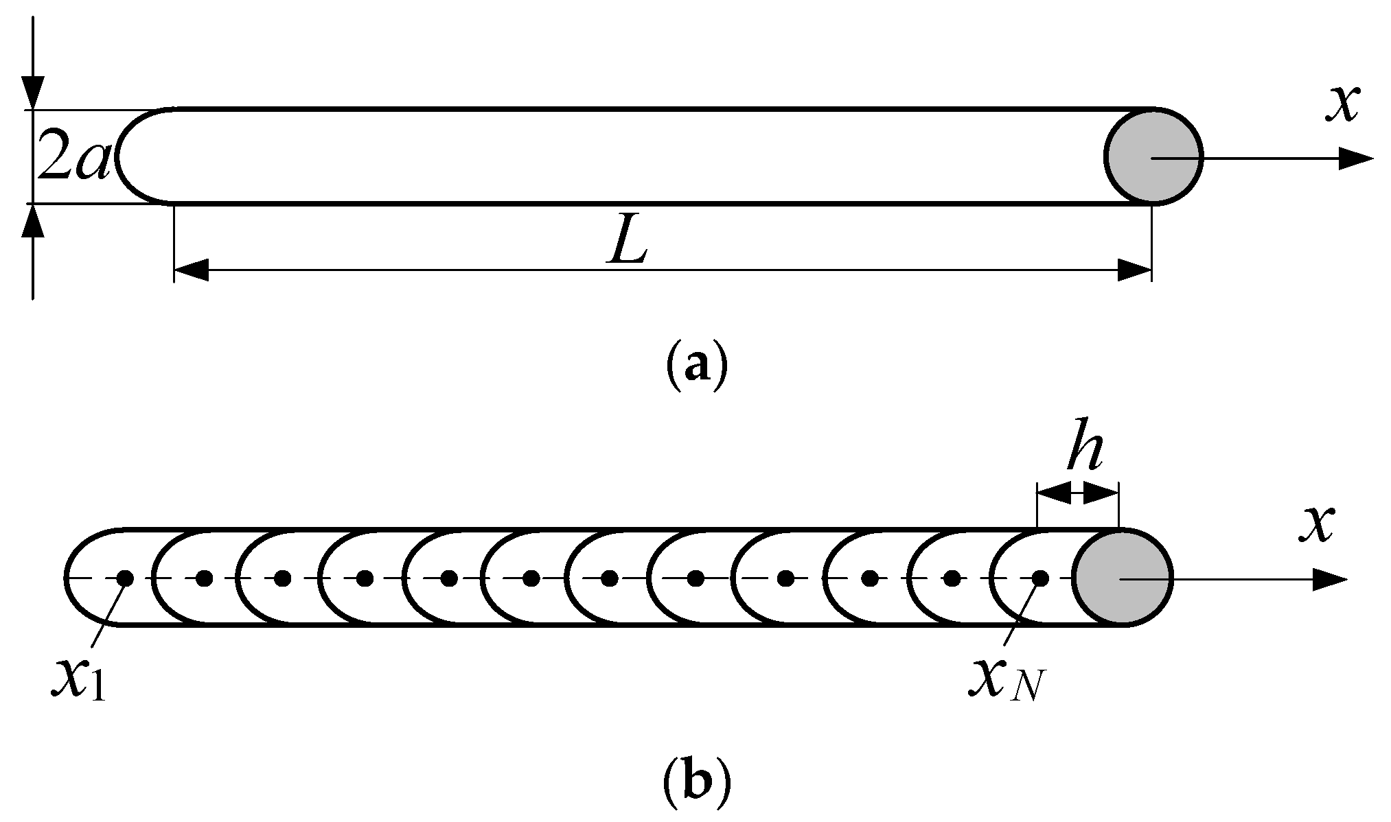
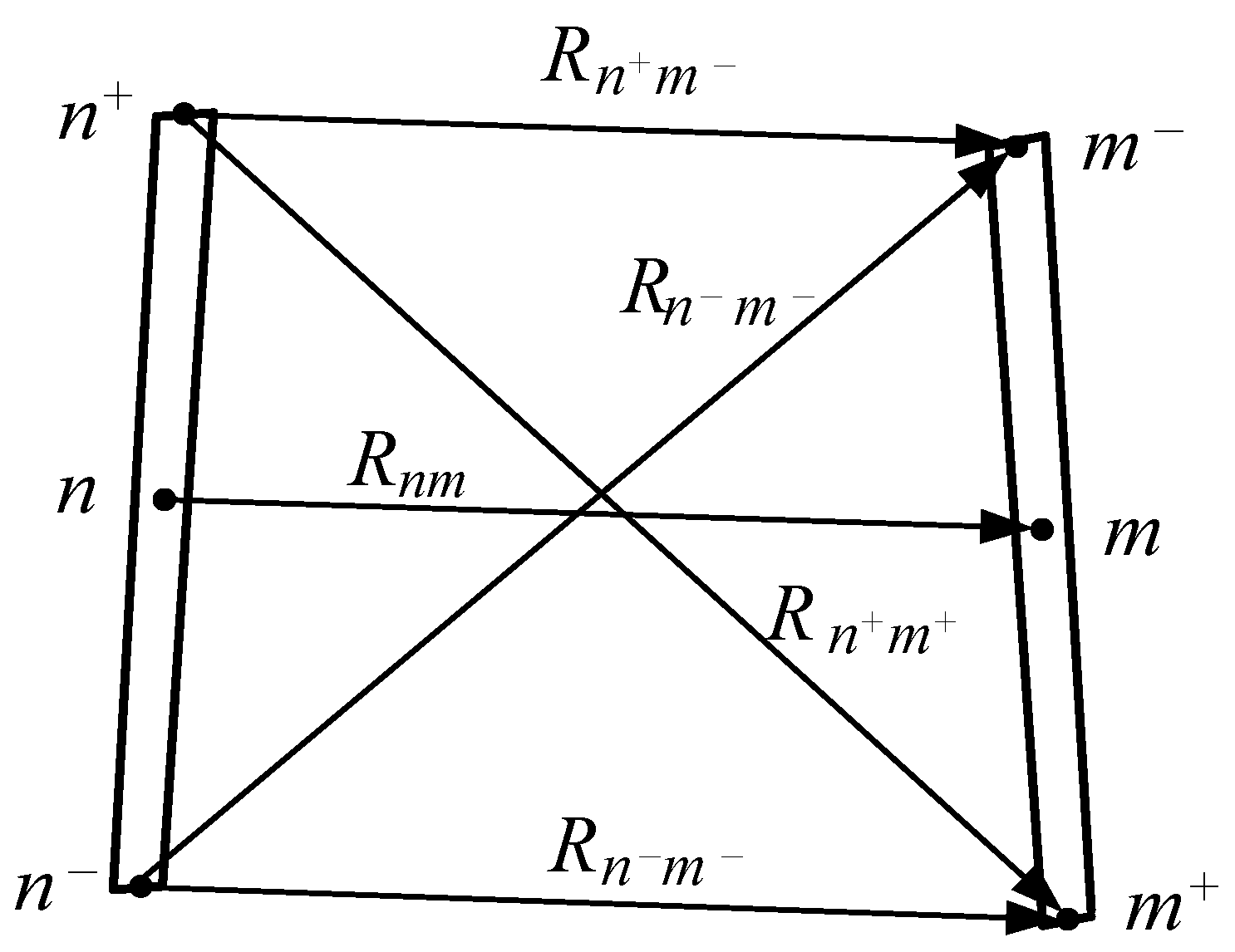
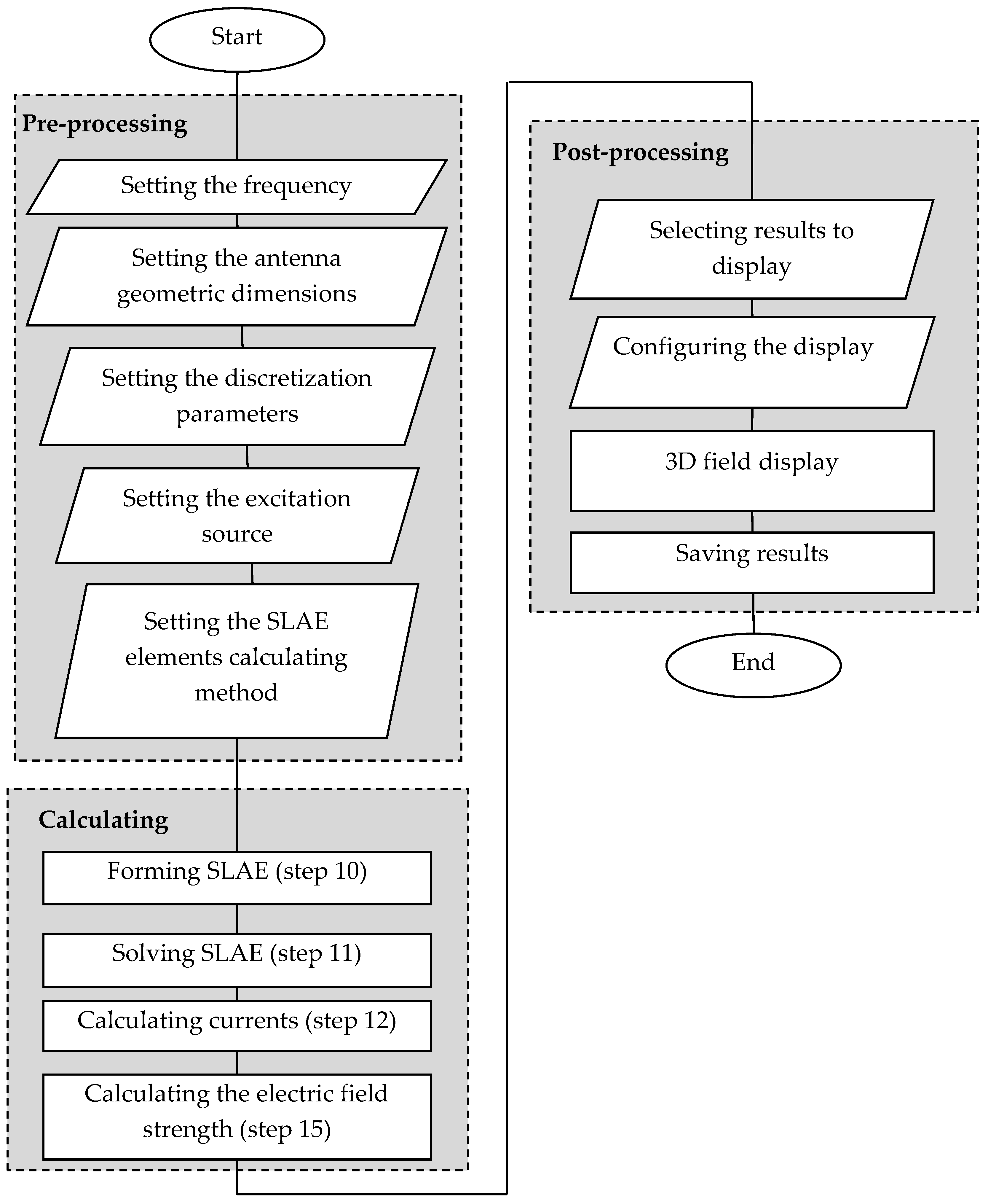
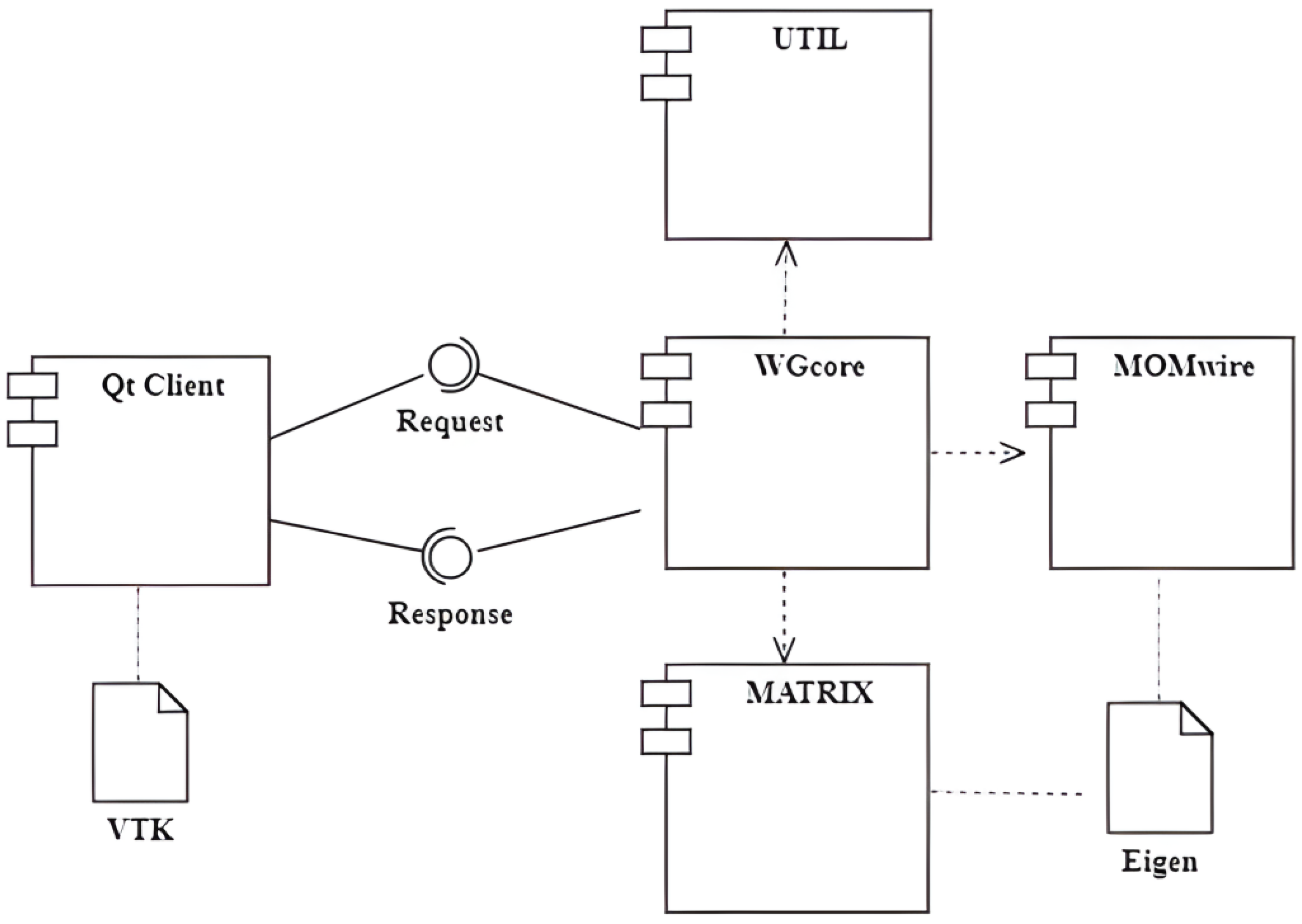
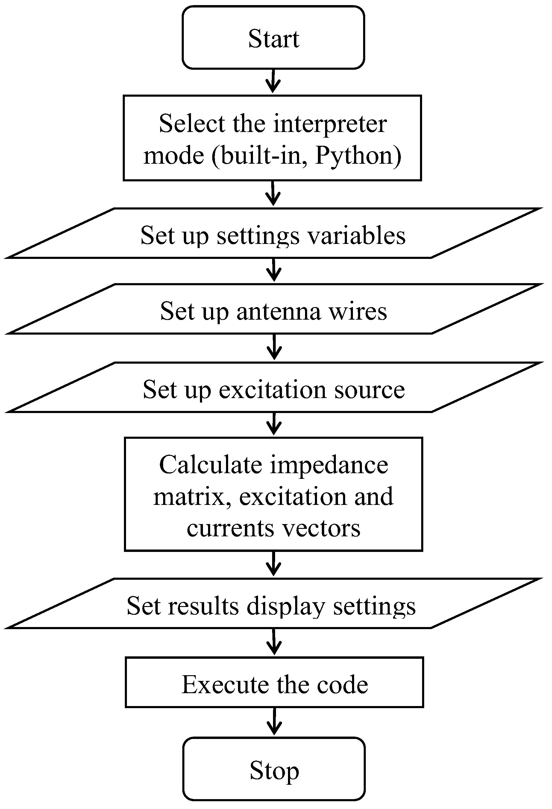
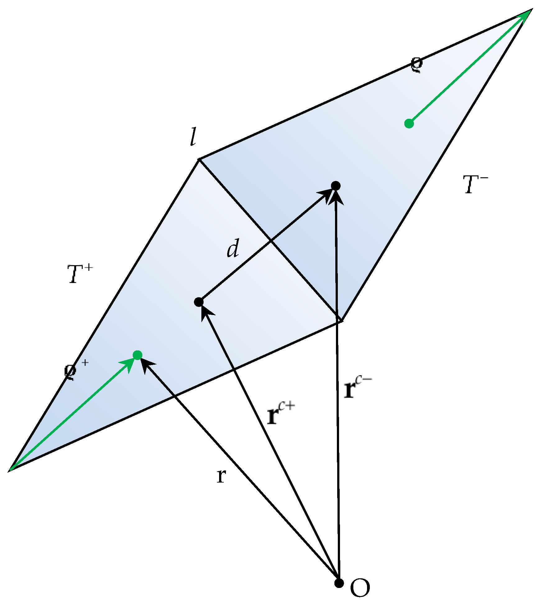
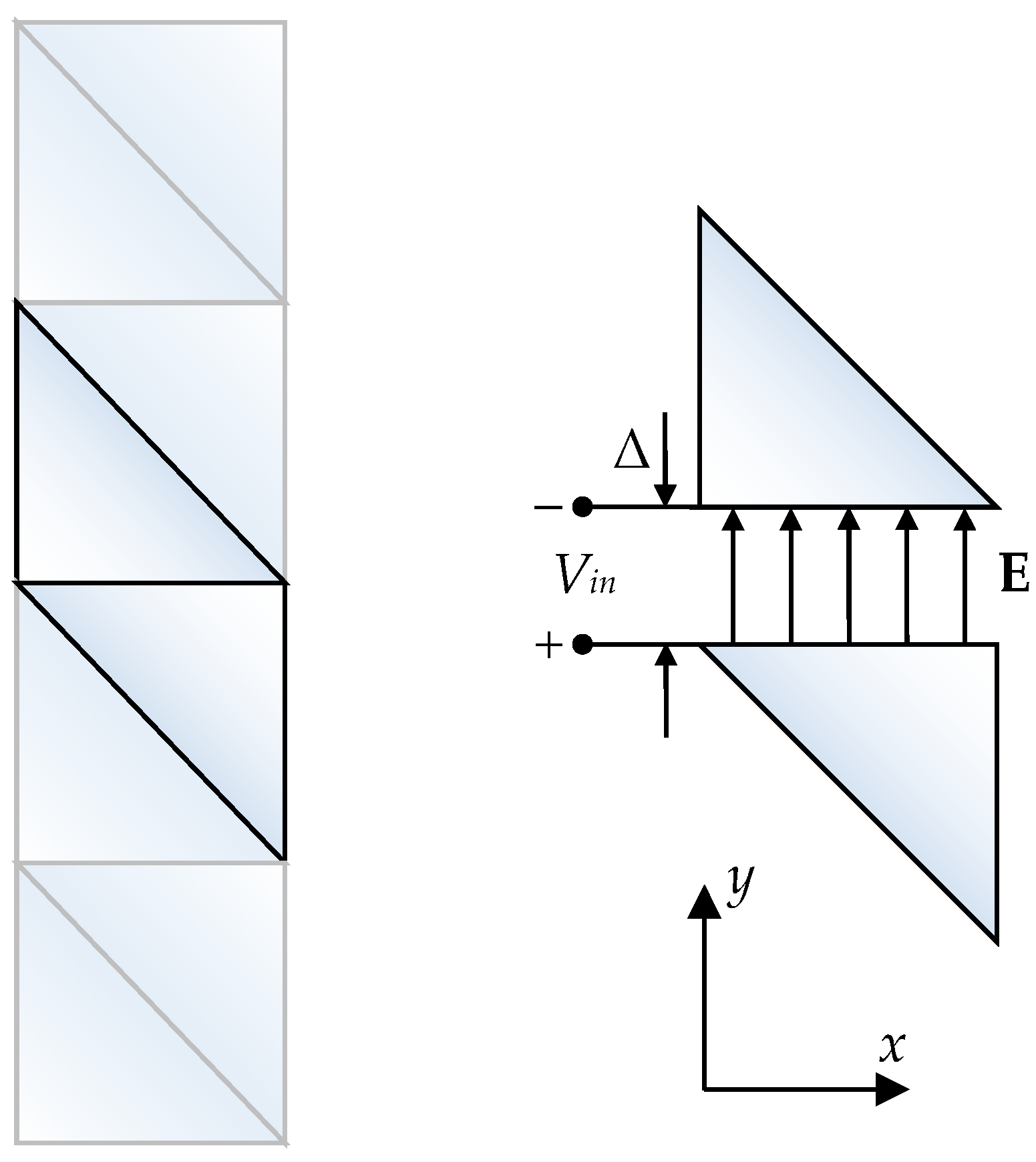
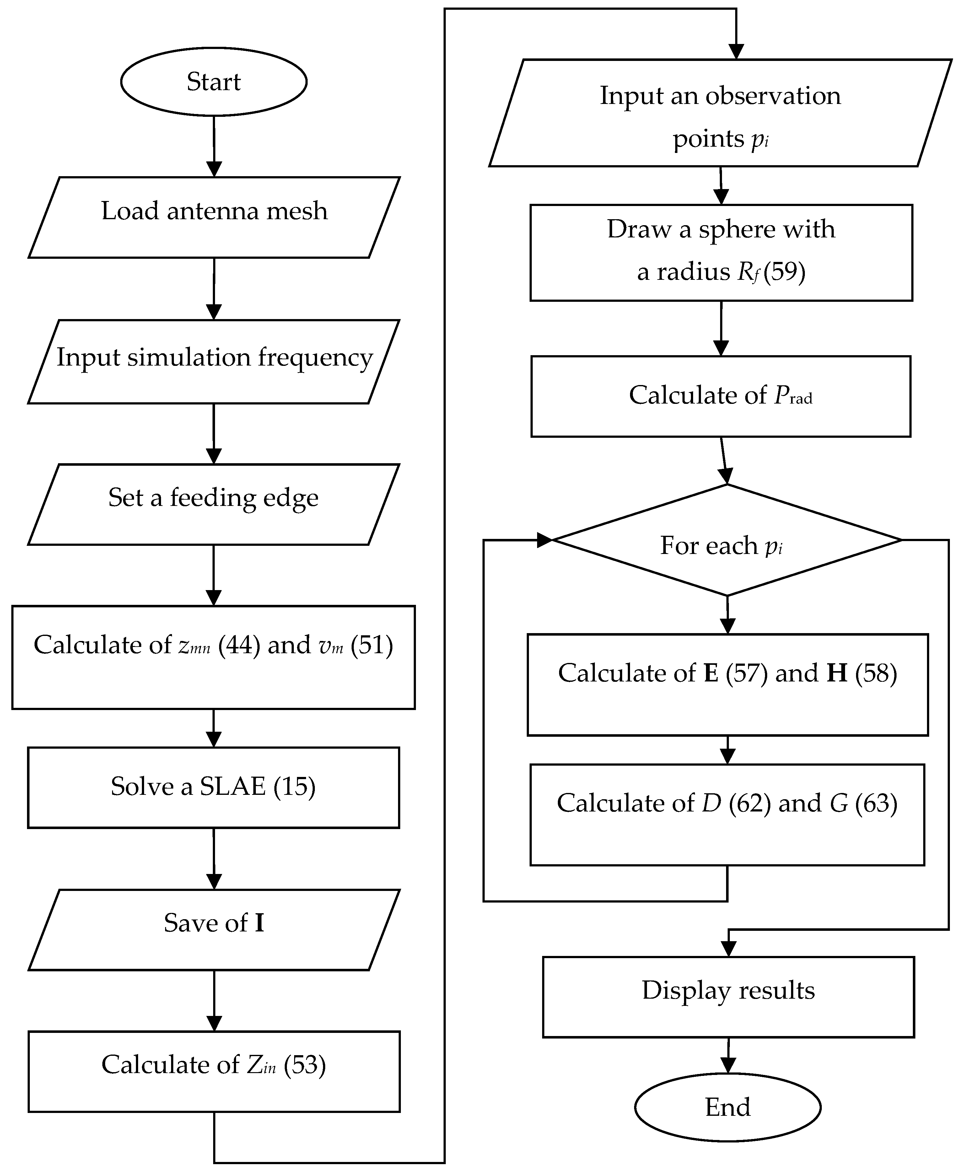
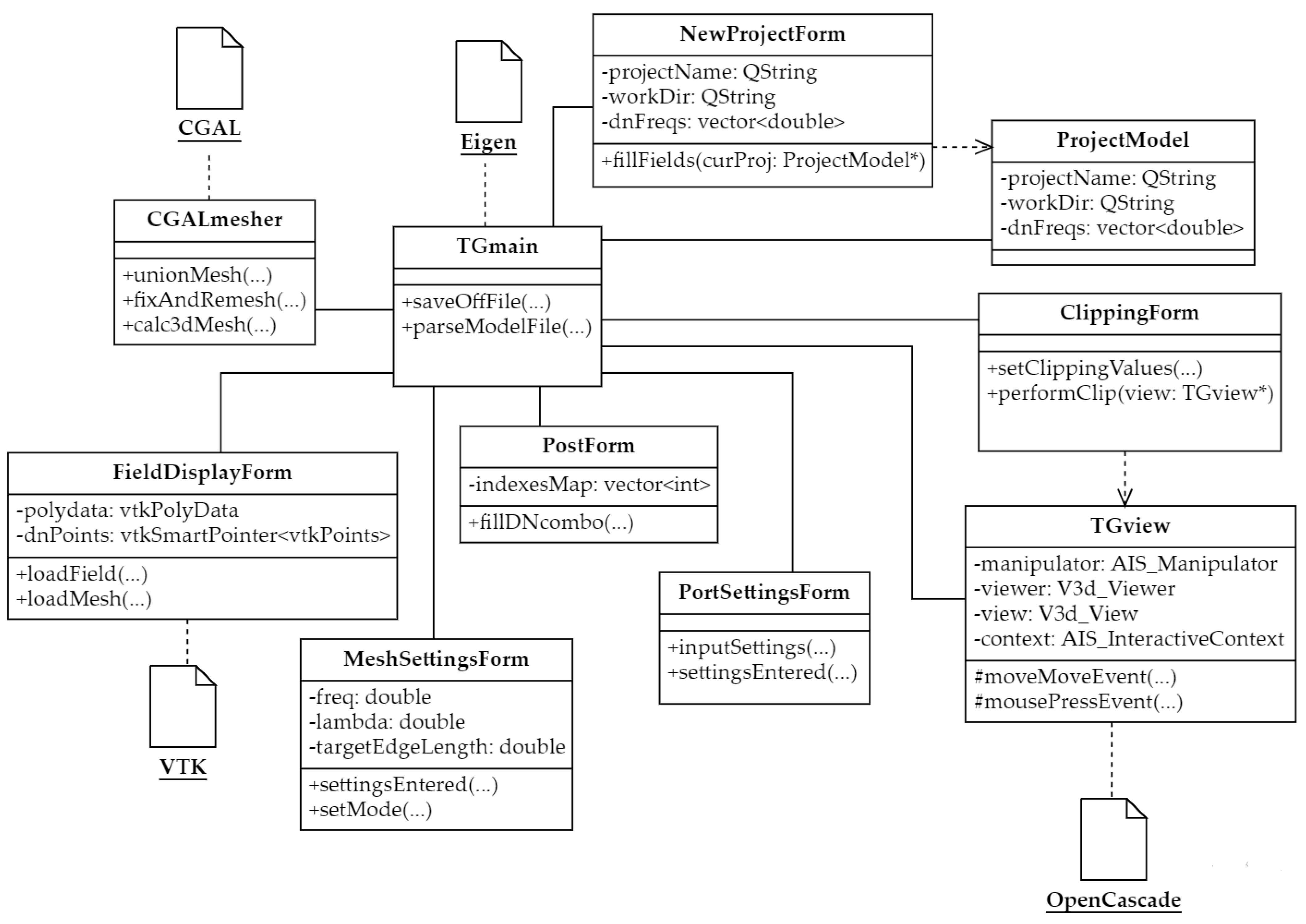
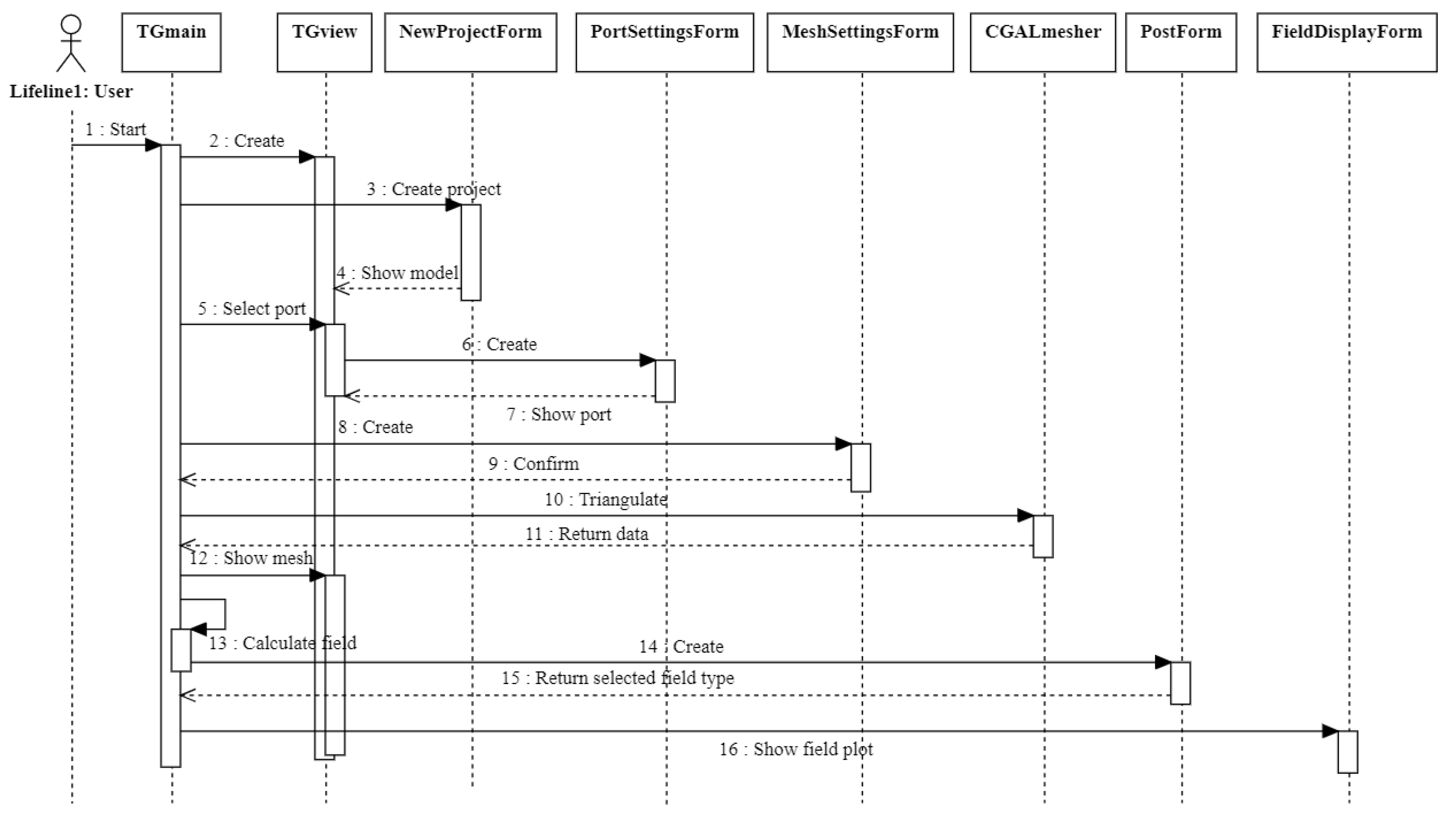
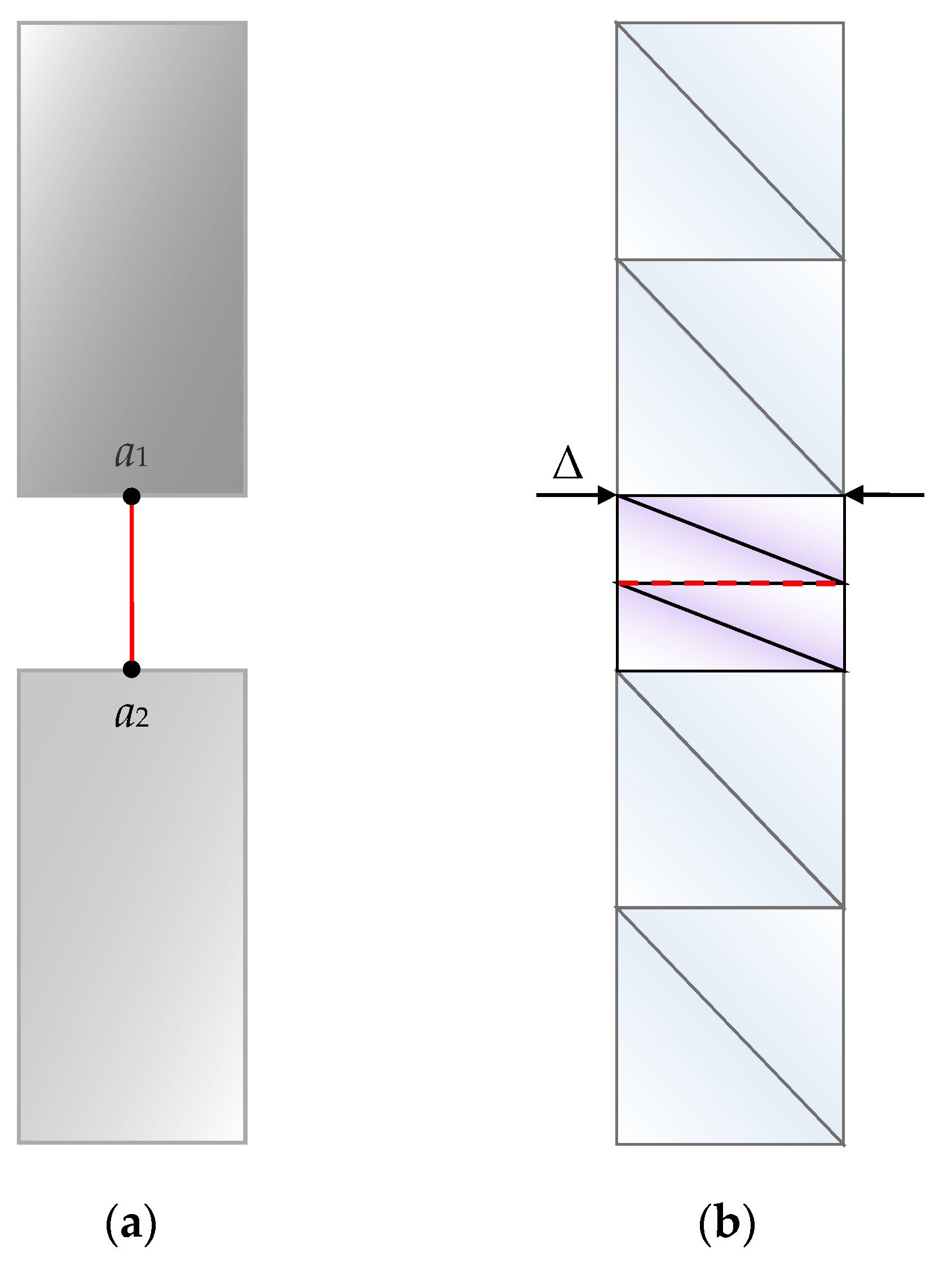
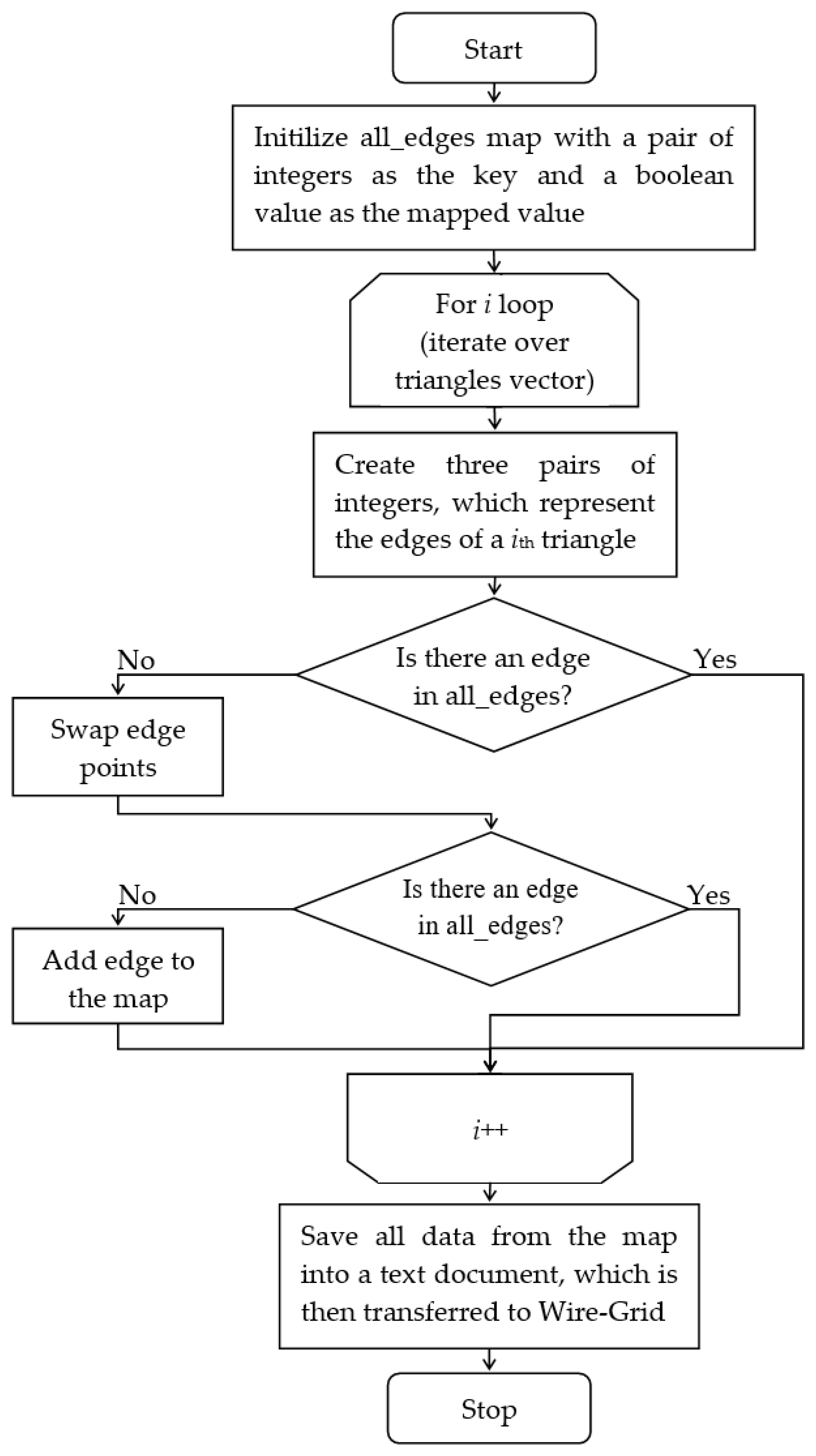
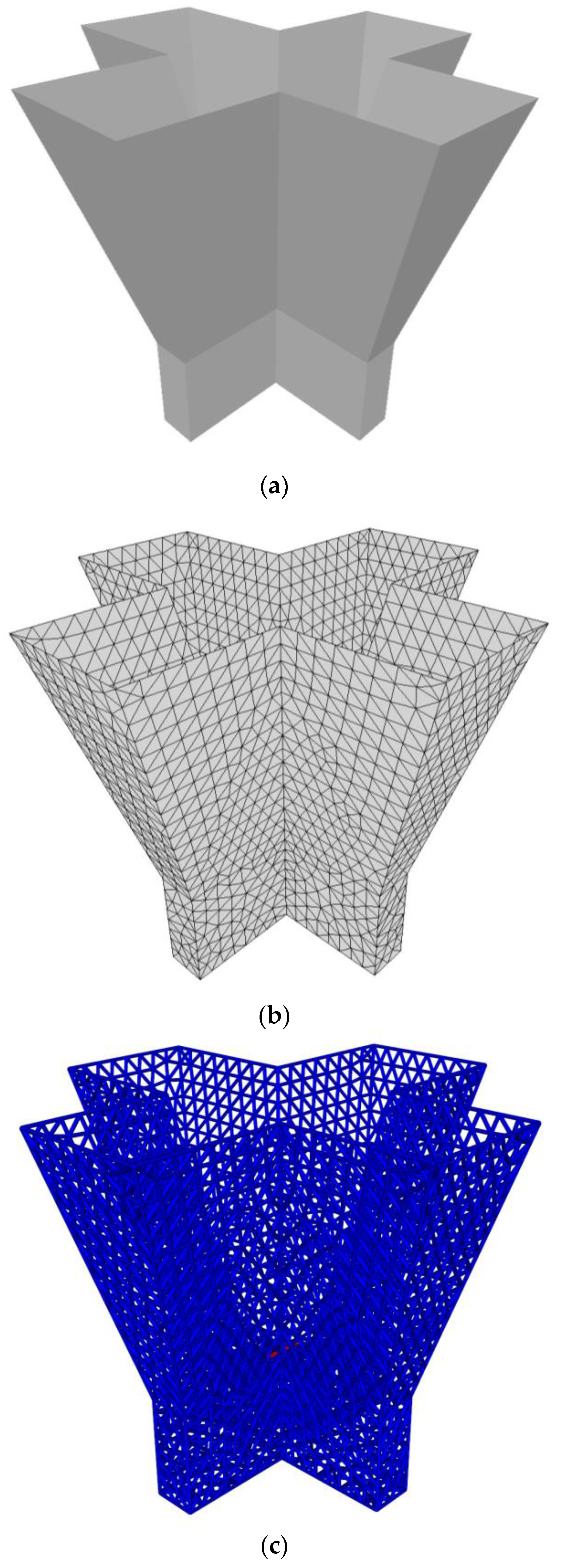
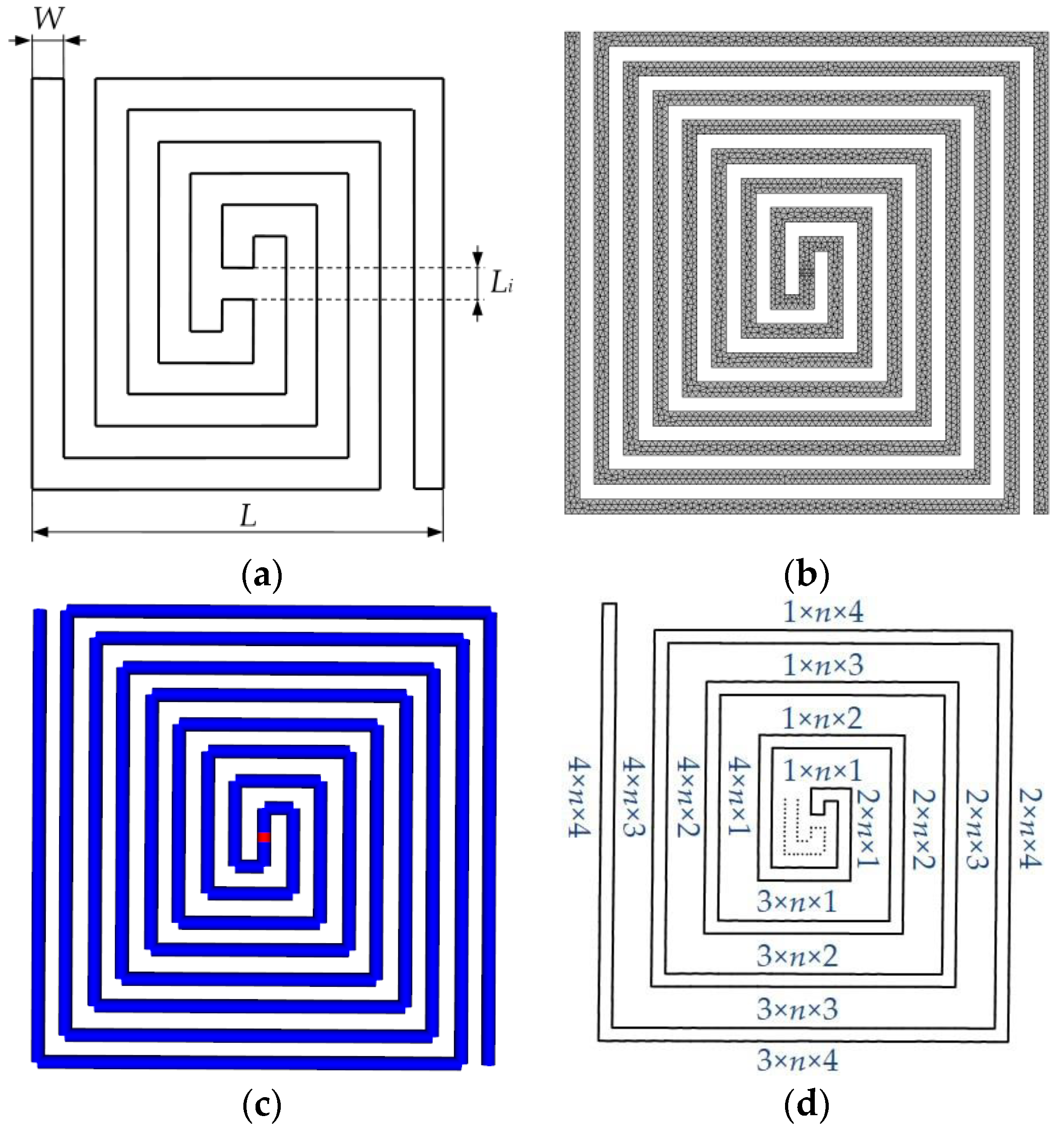
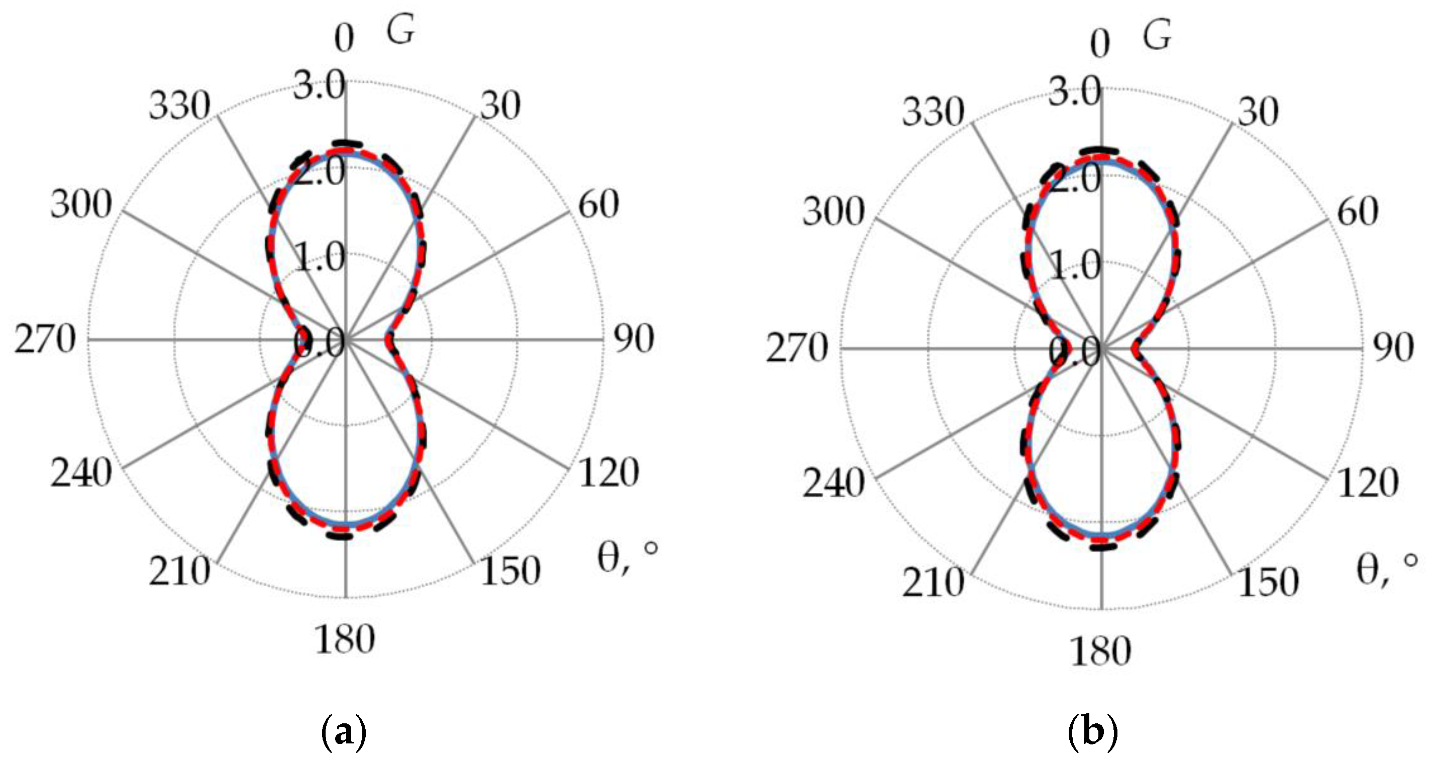
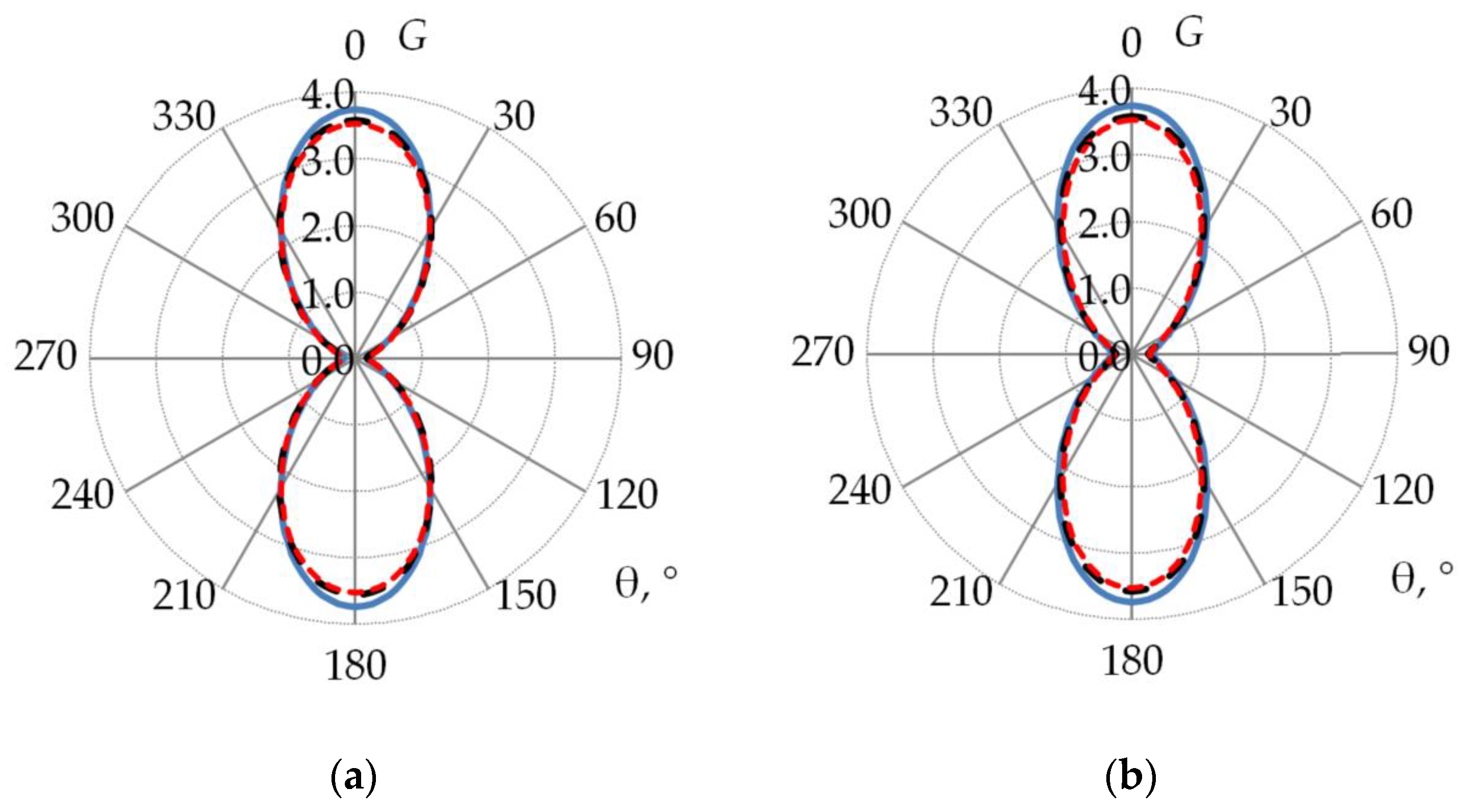
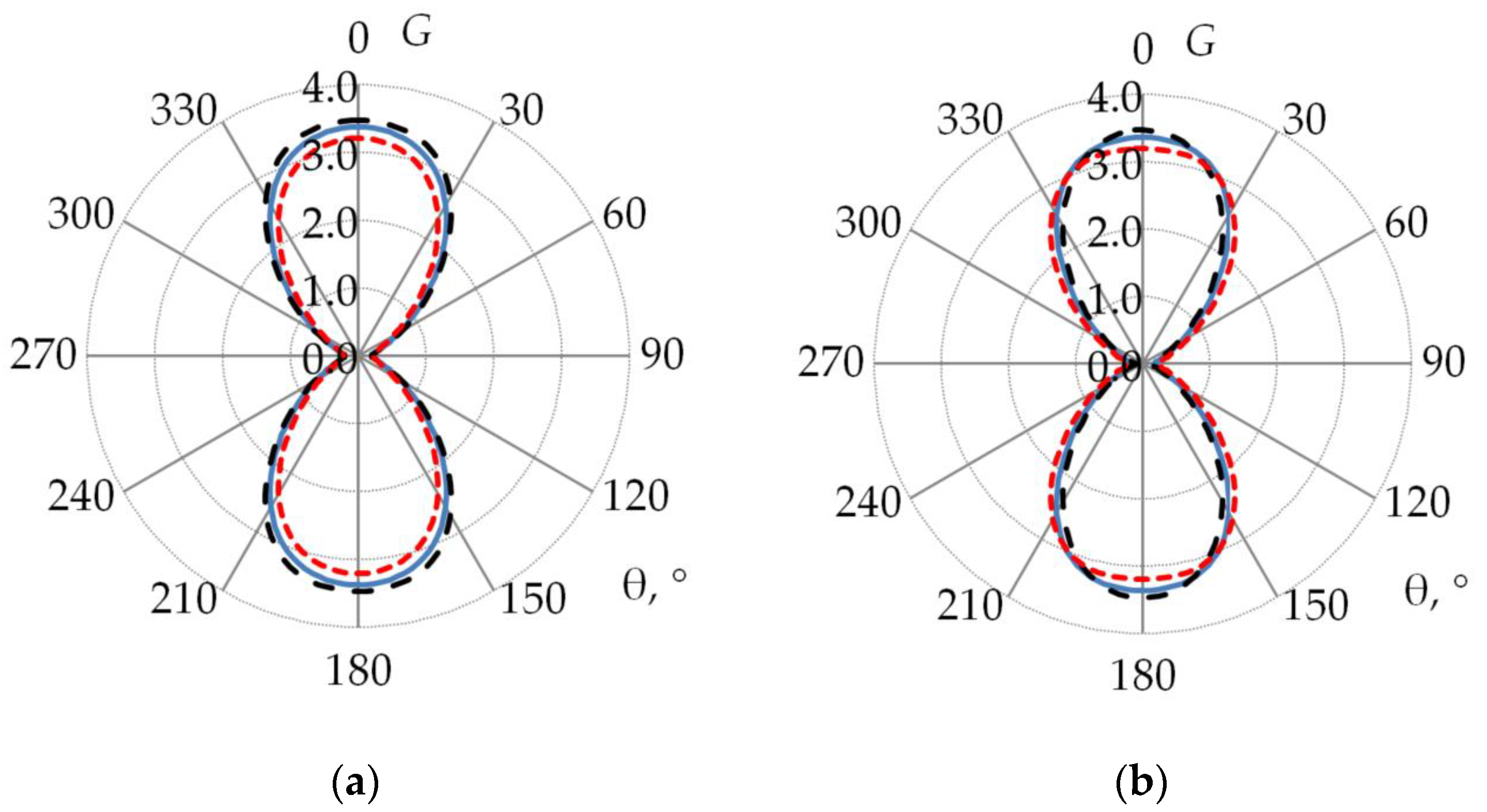
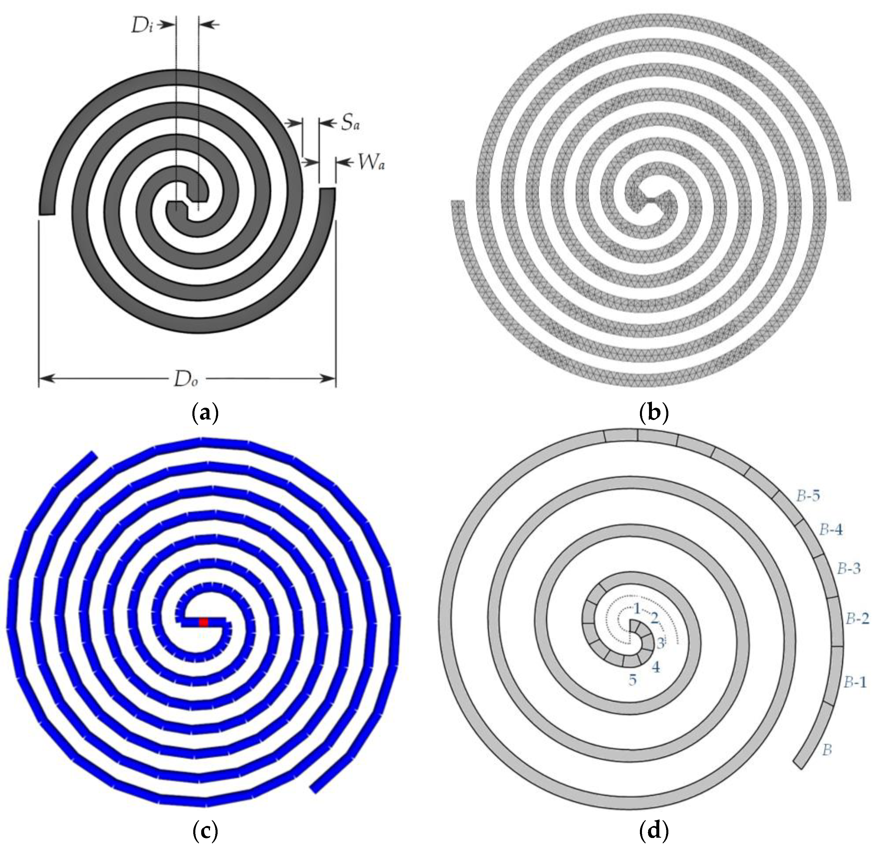
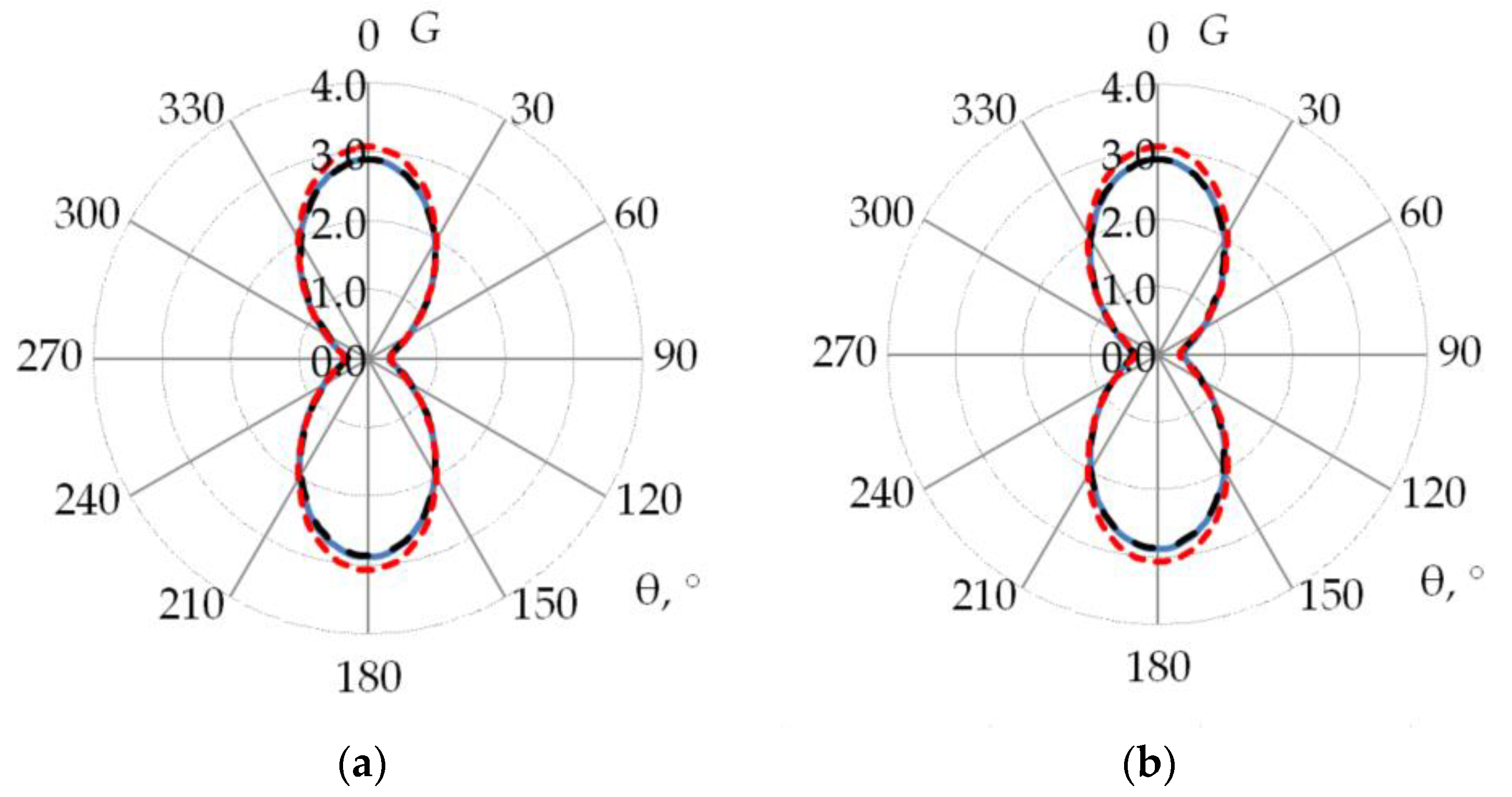
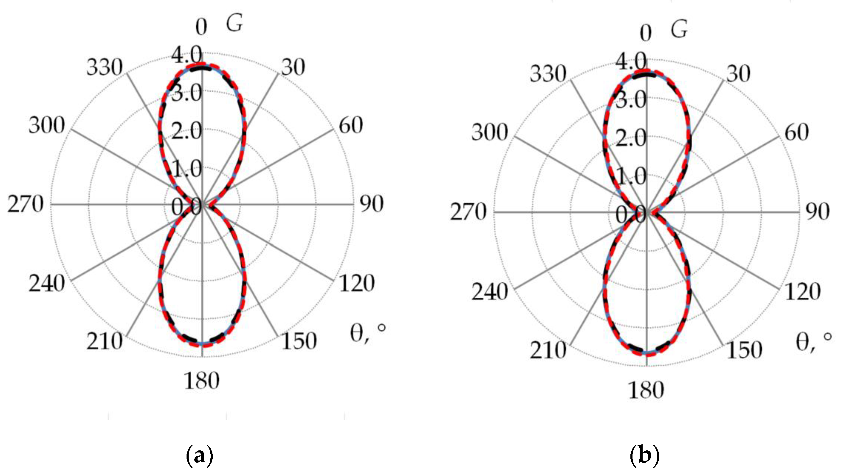
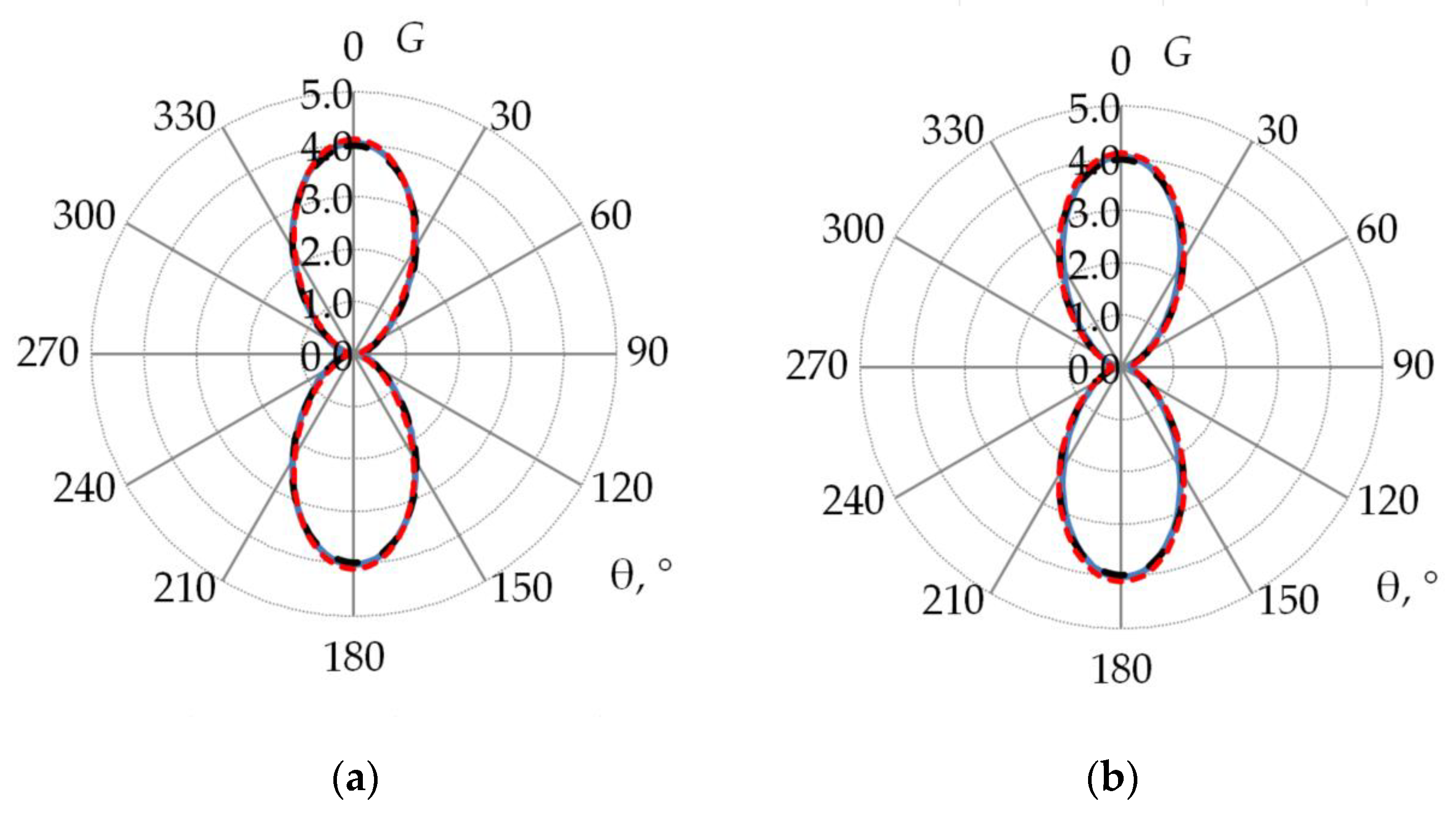
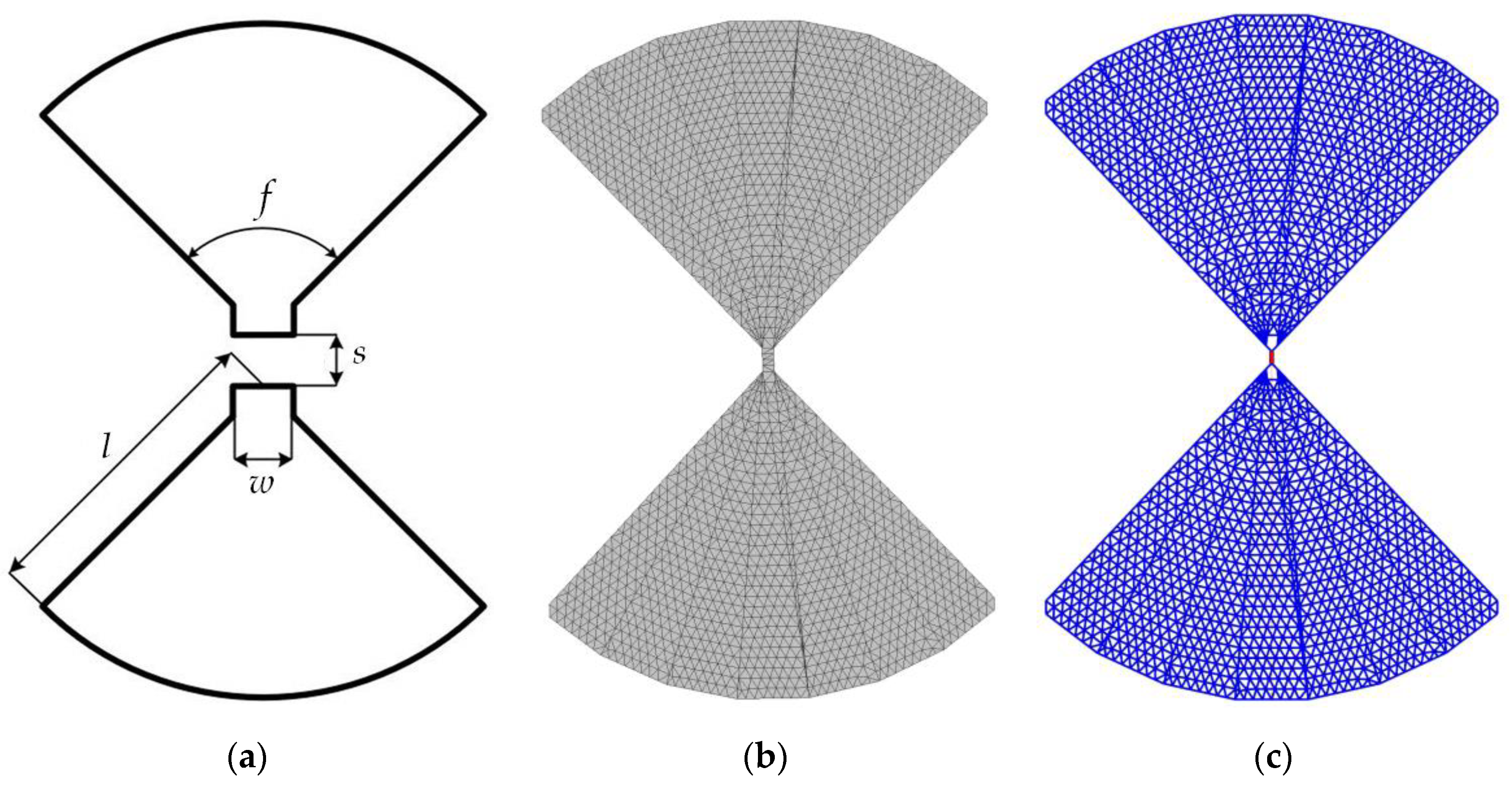
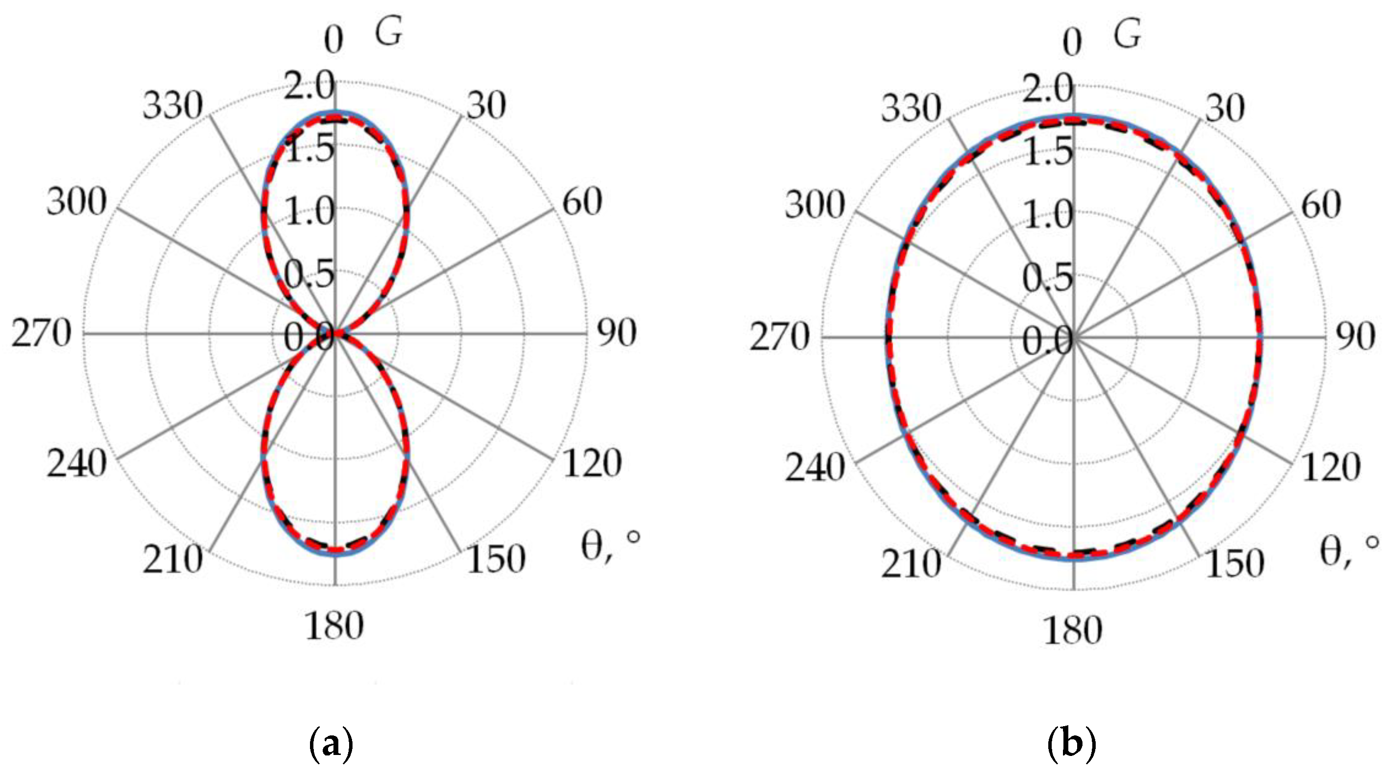
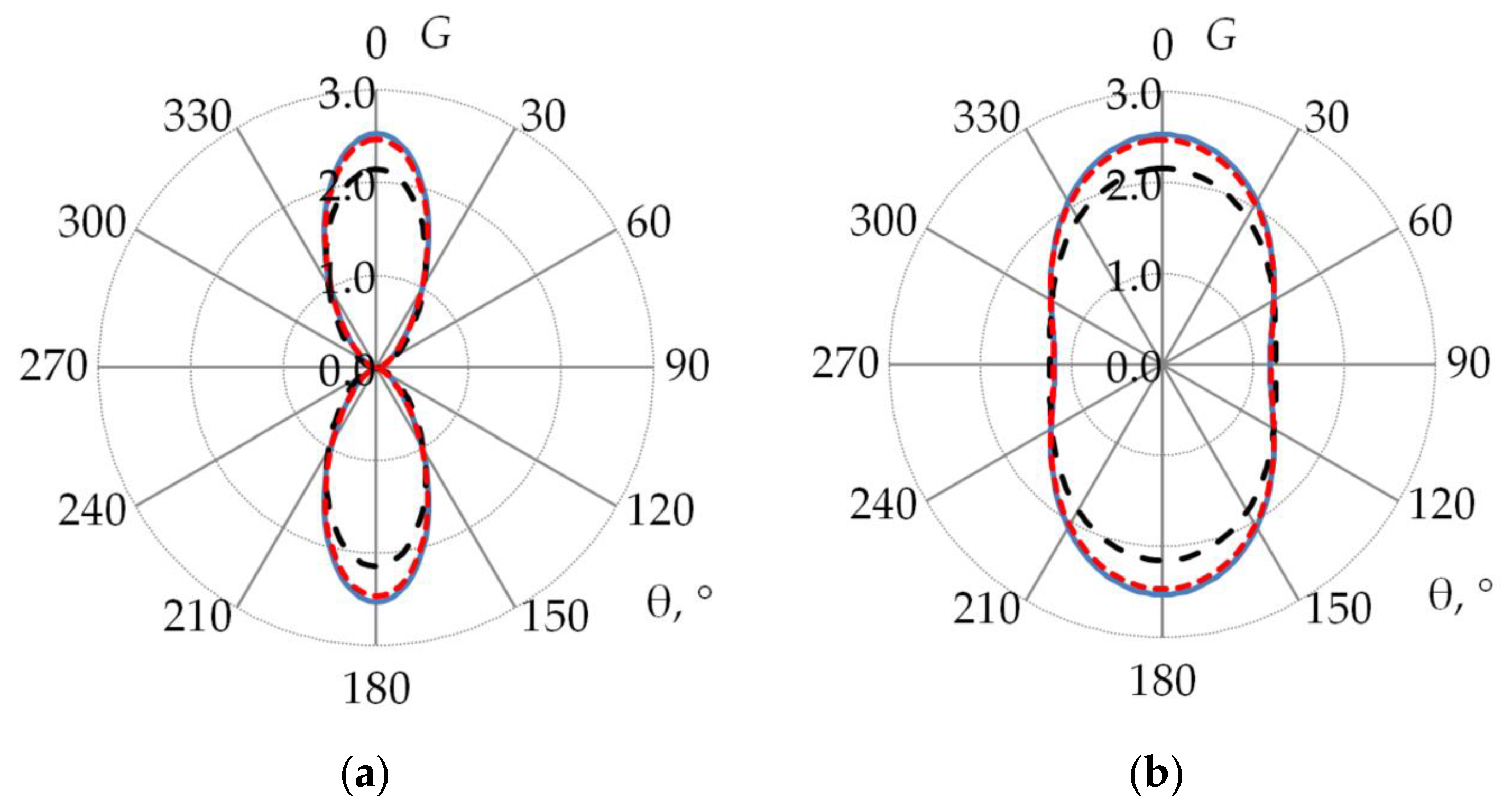
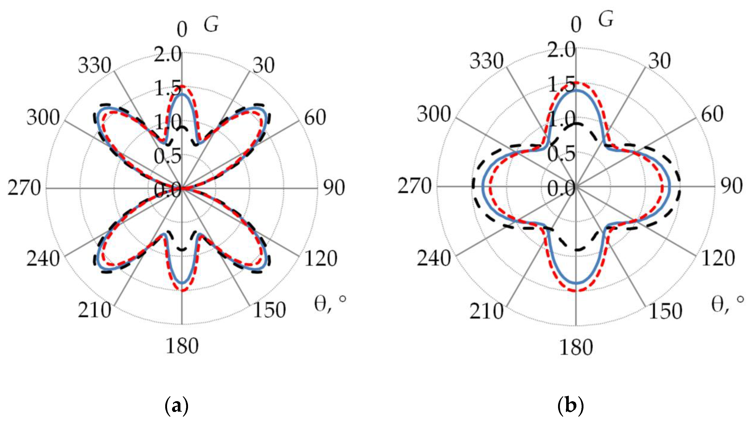
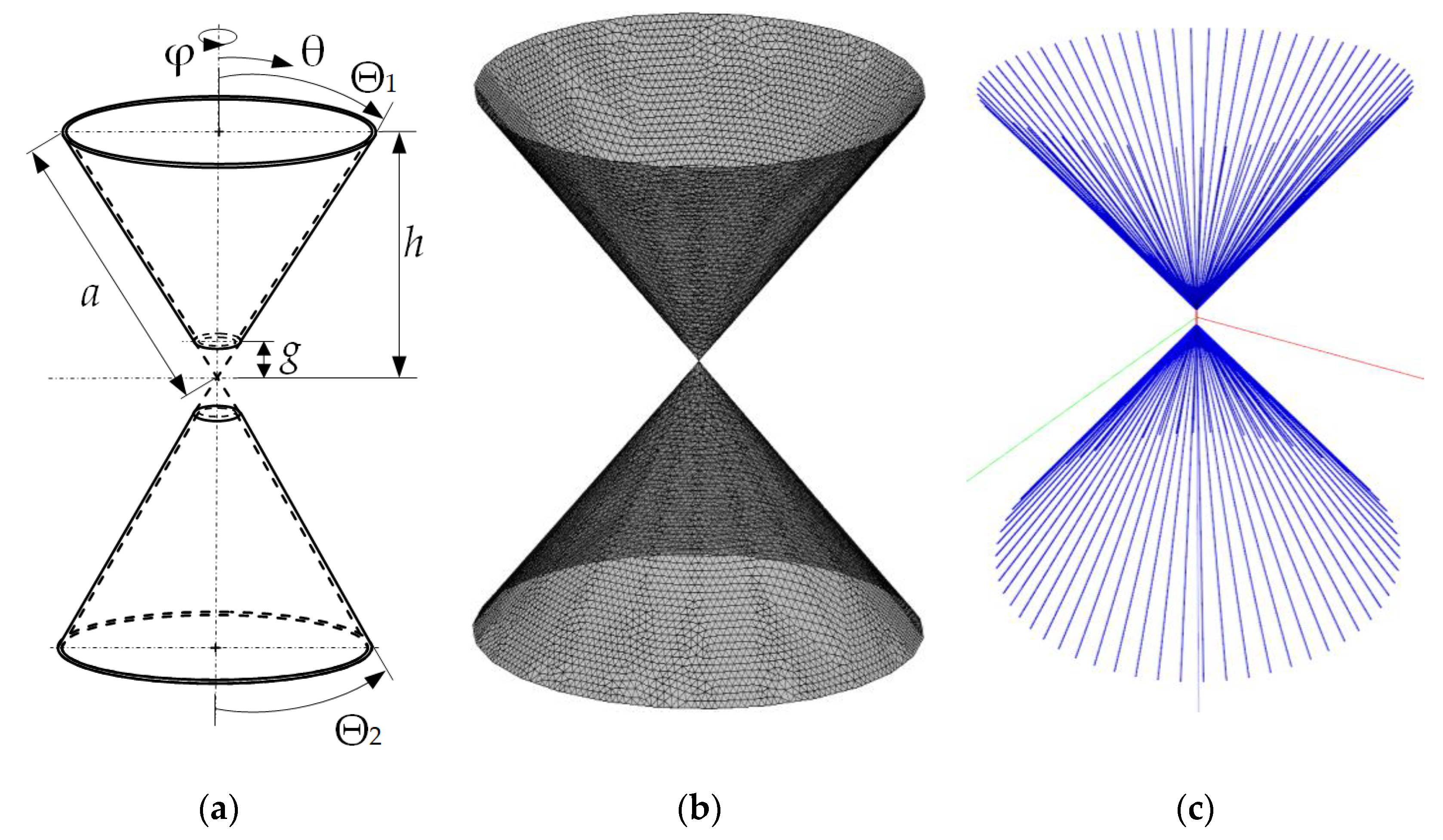
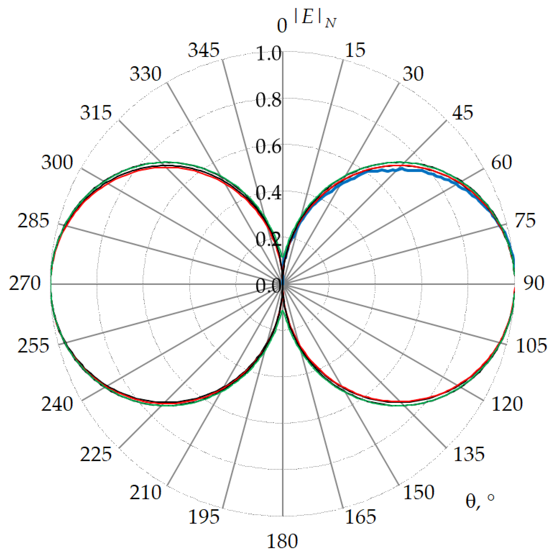
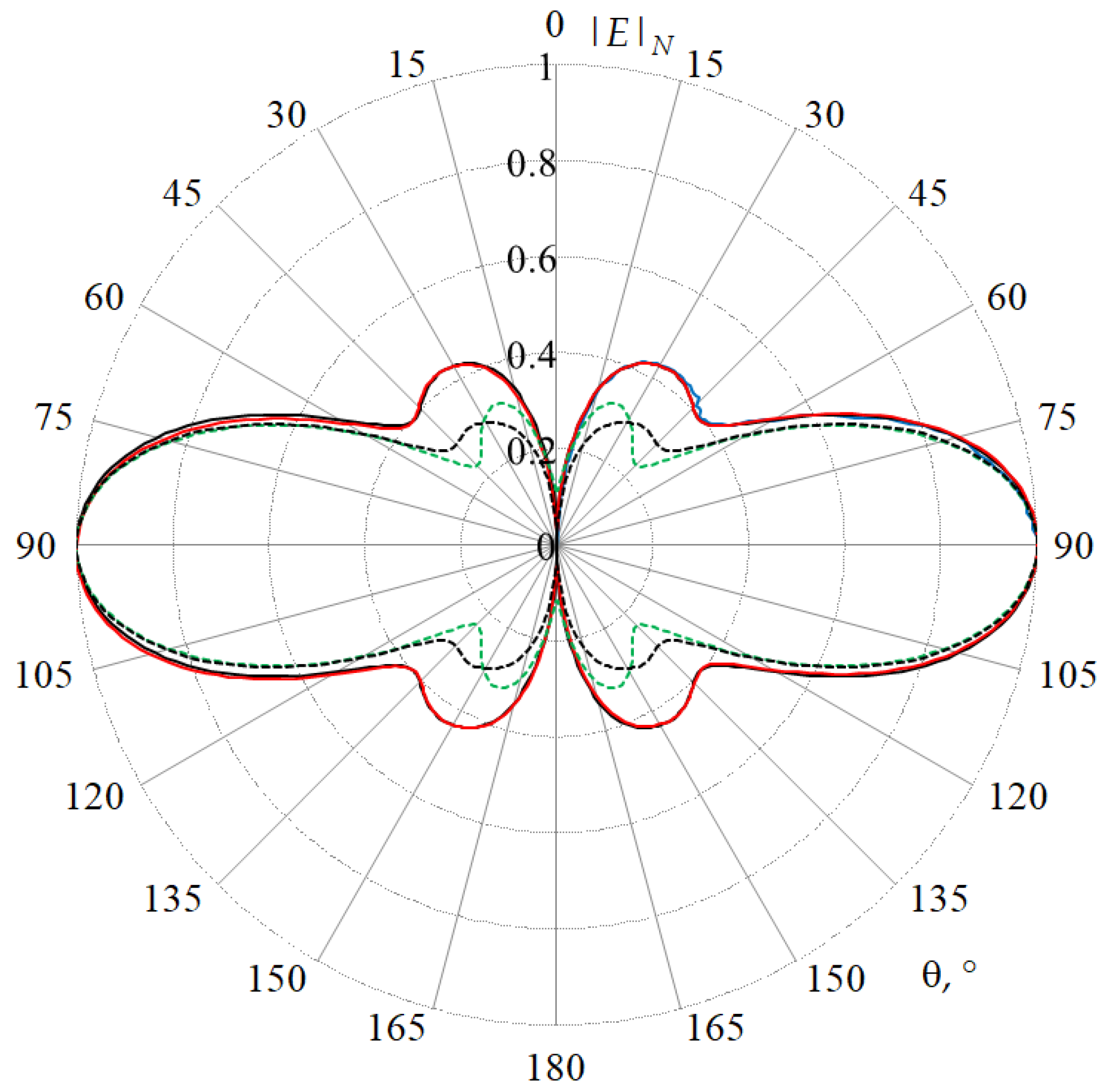
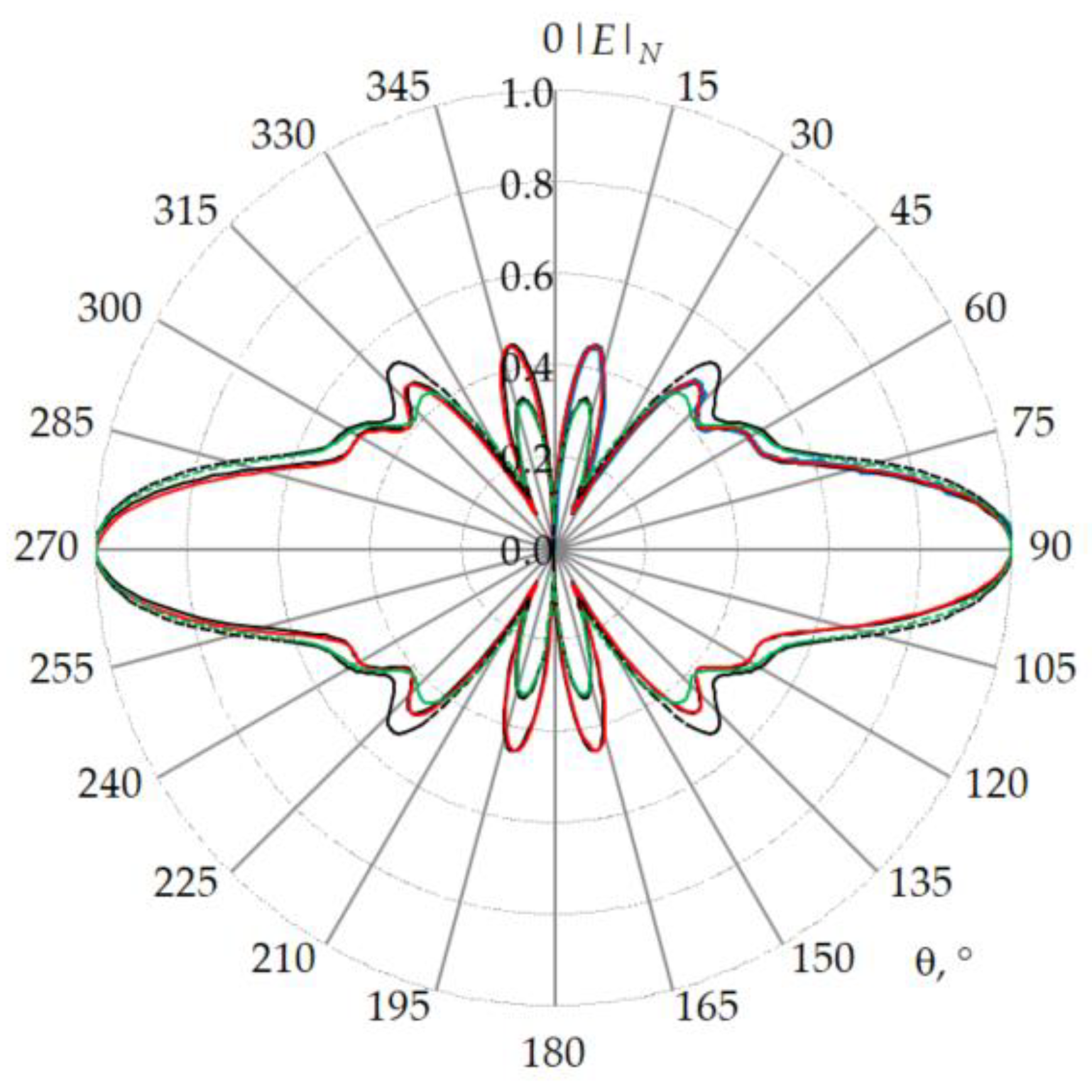
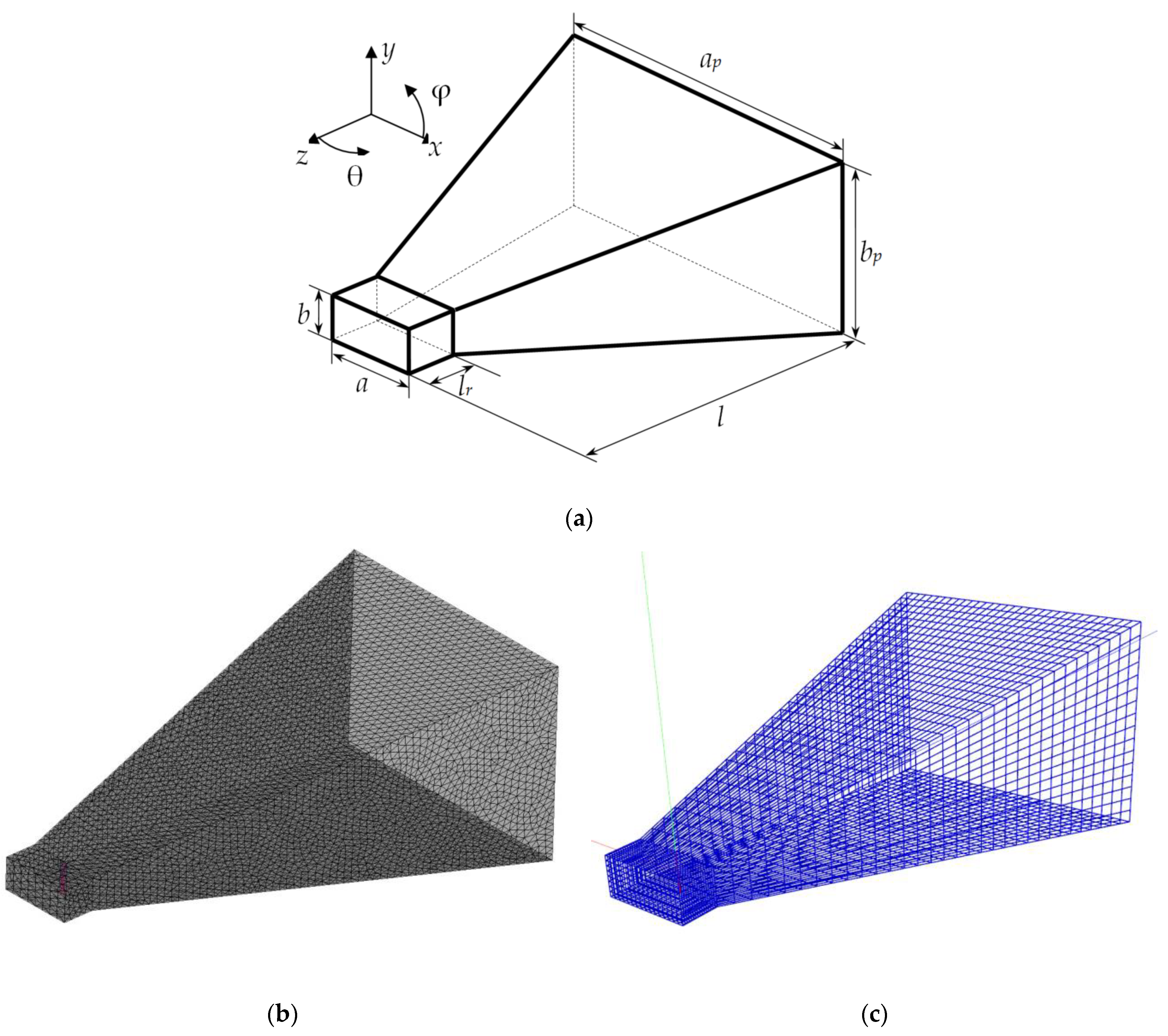
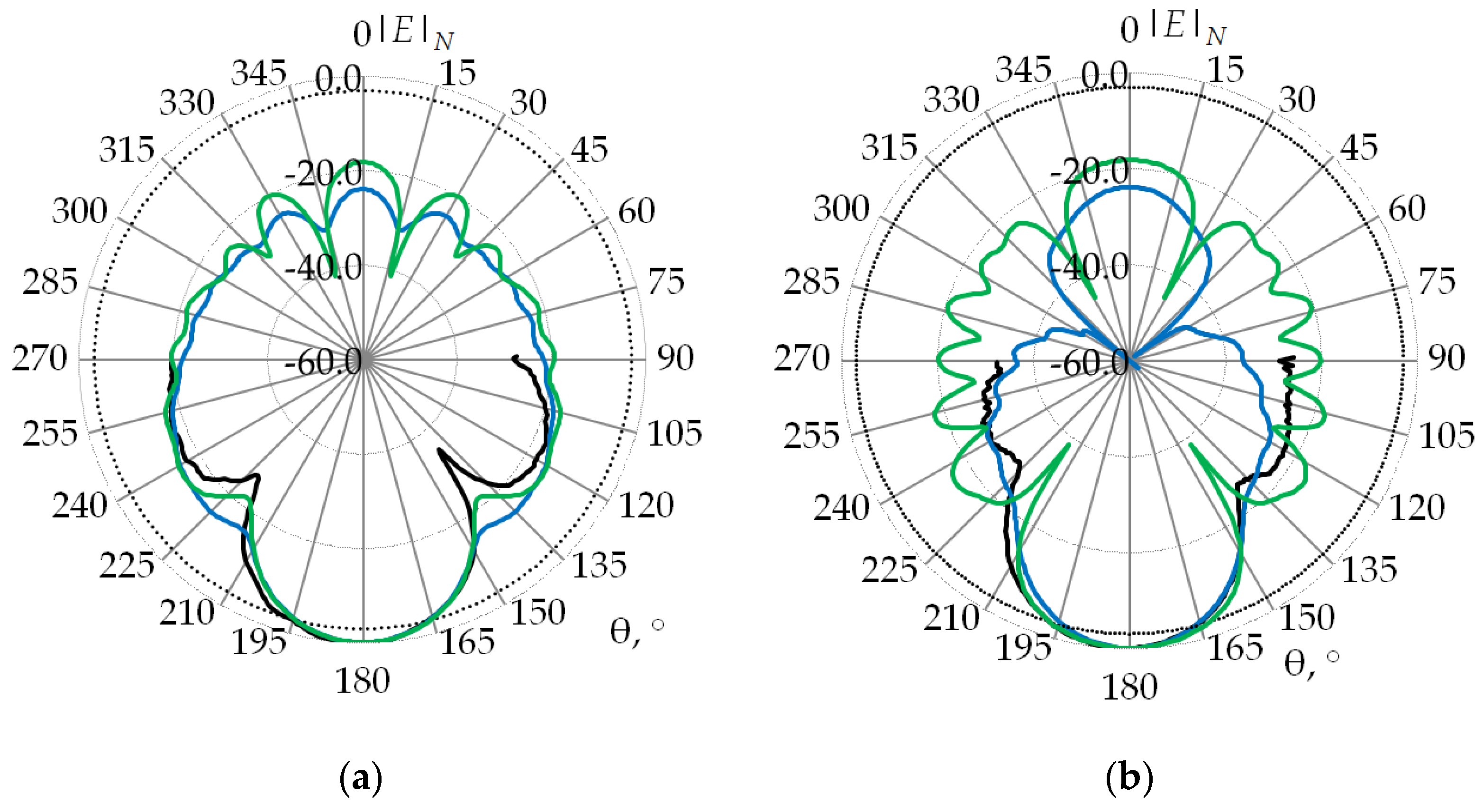
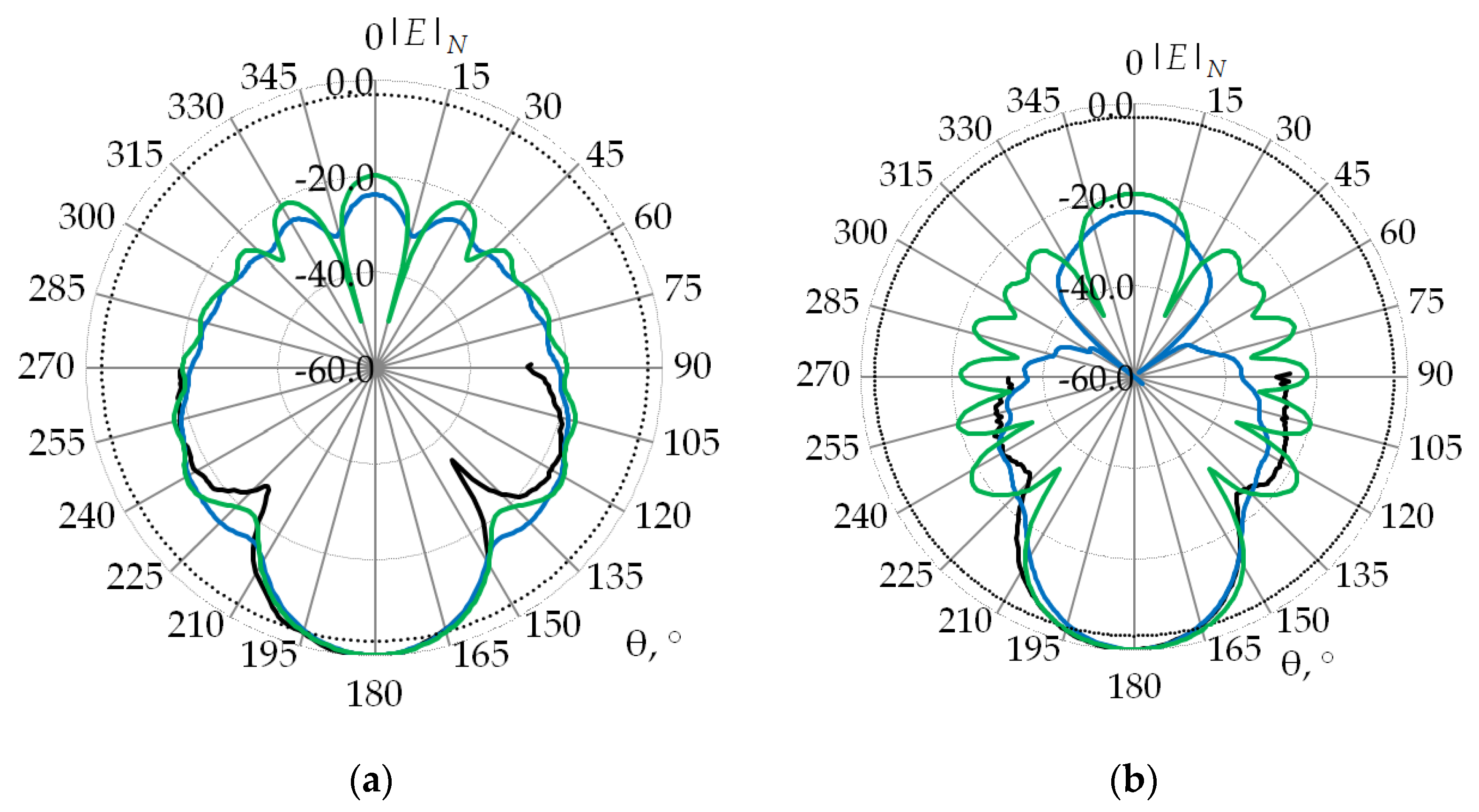
Figure 1. General view (a) and segmentation of a thin wire (b).
Algorithms 16 00200 g001
Figure 2. Separate segments n and m of the wires and the distances between them.
Algorithms 16 00200 g002
Figure 3. Block diagram of the Wire-Grid algorithm.
Algorithms 16 00200 g003
Figure 4. UML component diagram of the Wire-Grid.
Algorithms 16 00200 g004
Figure 5. Workflow of the Wire-Grid antenna modeling process.
Algorithms 16 00200 g005
Figure 6. RWG basis function defined for a pair of adjacent triangles.
Algorithms 16 00200 g006
Figure 7. Feeding edge model.
Algorithms 16 00200 g007
Figure 8. Antenna simulation algorithm based on triangular surface approximation and RWG basis functions.
Algorithms 16 00200 g008
Figure 9. UML component-diagram of the Triangle-Grid.
Algorithms 16 00200 g009
Figure 10. UML sequence-diagram of the Triangle-Grid.
Algorithms 16 00200 g010
Figure 11. Setting the length (a) and width (b) of the conductive plate used as an excitation source.
Algorithms 16 00200 g011
Figure 12. Block diagram of the mesh import function from Triangle-Grid to Wire-Grid.
Algorithms 16 00200 g012
Figure 13. Structure of a four waveguide-fed horn antenna (a) and its mesh using Triangle-Grid (b) and import function (c).
Algorithms 16 00200 g013
Figure 14. Top view of the planar rectangular spiral antenna (a), its constructed meshed model in Triangle-Grid (b), the model in Wire-Grid (the red wire is the excitation source) (c), and its adaptive segmentation model (d).
Algorithms 16 00200 g014
Figure 15. RPs of the planar rectangle spiral antenna at a frequency of 1 GHz in the E (a) and H (b) planes: Triangle-grid (- - -), Wire-grid (- - -) and EMPro (––).
Algorithms 16 00200 g015
Figure 16. RPs of the planar rectangle spiral antenna at a frequency of 3 GHz in the E (a) and H (b) planes: Triangle-grid (- - -), Wire-grid (- - -) and EMPro (––).
Algorithms 16 00200 g016
Figure 17. RPs of the planar rectangle spiral antenna at a frequency of 5 GHz in the E (a)and H (b) planes: Triangle-grid (- - -), Wire-grid (- - -) and EMPro (––).
Algorithms 16 00200 g017
Figure 18. Top view of the spiral antenna (a), and its constructed grid in Triangle-Grid (b) and in Wire-Grid (the red wire is the excitation source) (c), and its adaptive segmentation model (d).
Algorithms 16 00200 g018
Figure 19. RPs of the spiral antenna at a frequency of 1 GHz in the E (a) and H (b) planes: Triangle-grid (- - -), Wire-grid (- - -) and EMPro (––).
Algorithms 16 00200 g019
Figure 20. RPs of the spiral antenna at a frequency of 1.5 GHz in the E (a) and H (b) planes: Triangle-grid (- - -), Wire-grid (- - -) and EMPro (––).
Algorithms 16 00200 g020
Figure 21. RPs of the spiral antenna at a frequency of 2 GHz in the E (a) and H (b) planes: Triangle-grid (- - -), Wire-grid (- - -) and EMPro (––).
Algorithms 16 00200 g021
Figure 22. Top view of the bow-tie antenna (a), and its constructed grid in Triangle-Grid (b) and in Wire-Grid using the import function for meshing (c).
Algorithms 16 00200 g022
Figure 23. RPs of the planar bow-tie antenna at a frequency of 0.5 GHz in the E (a) and H (b) planes: Triangle-grid (- - -), Wire-grid (- - -) and EMPro (––).
Algorithms 16 00200 g023
Figure 24. RPs of the planar bow-tie antenna at a frequency of 1 GHz in the E (a) and H (b) planes: Triangle-grid (- - -), Wire-grid (- - -) and EMPro (––).
Algorithms 16 00200 g024
Figure 25. RPs of the planar bow-tie antenna at a frequency of 1.5 GHz in the E (a) and H (b) planes: Triangle-grid (- - -), Wire-grid (- - -) and EMPro (––).
Algorithms 16 00200 g025
Figure 26. Isometric view of the biconical antenna (a), and its constructed gridin Triangle-Grid (b) and in Wire-Grid (the red wire is the excitation source) (c).
Algorithms 16 00200 g026
Figure 27. RPs of the biconical antenna at a frequency of 0.1 GHz in the E plane: Triangle-grid (- - -), Wire-grid (- - -), digitalized from Samaddar 1998 (––), analytically by Papas 1951 (––) and Samaddar 1998 (––).
Algorithms 16 00200 g027
Figure 28. RPs of the biconical antenna at a frequency of 0.5 GHz in the E plane: Triangle-grid (- - -), Wire-grid (- - -), digitalized from Samaddar 1998 (––), analytically by Papas 1951 (––) and Samaddar 1998 (––).
Algorithms 16 00200 g028
Figure 29. RPs of the biconical antenna at a frequency of 1 GHz in the E plane: Triangle-grid (- - -), Wire-grid (- - -), digitalized from Samaddar 1998 (––), analytically by Papas 1951 (––) and Samaddar 1998 (––).
Algorithms 16 00200 g029
Figure 30. Isometric view of the horn antenna (a), and its constructed grid in Triangle-Grid (b) and in Wire-Grid (the red wire is the excitation source) (c).
Algorithms 16 00200 g030
Figure 31. RPs of the horn antenna at a frequency of 8 GHz in the E (a) and H (b) planes: Triangle-grid (––), Wire-grid (λ/40) (––), measurements [347] (––) and -3 dB level (- - -).
Algorithms 16 00200 g031
Figure 32. RPs of the horn antenna at a frequency of 8 GHz in the E (a) and H (b) planes: Triangle-grid (––), Wire-grid (λ/15) (––), measurements [347] (––) and -3 dB level (- - -).
Algorithms 16 00200 g032
Table 1. The maximum gain values of the planar rectangle spiral antenna and the percentage of their relative difference from EMPro.
CodeValue1 GHz3 GHz5 GHz
Wire-GridMaximum gain2.23.533.2
Triangle-GridMaximum gain2.283.573.47
EMProMaximum gain2.153.743.37
Wire-GridRD* −2%6%5%
Triangle-GridRD−6%5%−3%
* (−) indicates by what percent the value is bigger than the reference one (here EMPro).
Table 2. The input impedance values of the planar rectangle spiral antenna, obtained using different codes with the corresponding computational costs.
CodeFrequency (GHz)Impedance (Ohm)Memory (GB)Time (ms)NCond (Z)
Wire-Grid1113.0 − j37.2* ≈0.212548619.48 × 104
387.6 − j60.5≈0.181546891.16 × 104
5154.8 − j21.0≈0.16955174.40 × 103
Triangle-Grid1175.8 − j38.2≈0.153885771.96 × 104
3153.5 − j7.7≈0.4512,18735798.17 × 103
5209.5 + j19.4≈1.7197,04310,1455.09 × 104
EMPro1170.9 − j30.1≈0.04600038,808- **
3154.1 − j43.7≈0.1329,000164,604-
5143.6 + j88.1≈0.2791,000322,080-
* (≈) denotes that the value is approximately equal to these numbers. ** (-) denotes that the data are not available.
Table 3. The percentage of the relative difference between the considered input impedance values of the planar rectangle spiral antenna in Table 2 and EMPro.
CodeFrequency (GHz)RD Impedance (%)RD Memory (%)RD Time (%)
Wire-Grid131.44* −42595.77
333.53−38.4699.47
57.2740.7499.90
Triangle-Grid1−3.67−27593.53
34.05−246.1557.98
5−24.89−533.33−6.64
* (−) indicates by what percent the value is bigger than the reference one (here EMPro).
Table 4. The maximum gain values of the planar spiral antenna and the percentage of their relative difference from EMPro.
CodeValue1 GHz1.5 GHz2 GHz
Wire-GridMaximum gain3.073.724.09
Triangle-GridMaximum gain2.883.63.98
EMProMaximum gain2.893.664.03
Wire-GridRD * −6%−2%−1%
Triangle-GridRD 0%2%1%
* (−) indicates by what percent the value is bigger than the reference one (here EMPro).
Table 5. The input impedance values of the planar spiral antenna, obtained using different codes with the corresponding computational costs.
CodeFrequency (GHz)Impedance (Ohm)Memory (GB)Time (ms)NCond (Z)
Wire-Grid1156.0 + j15.4* ≈3.1528,37280153.02 × 1012
1.5194.3 − j8.6≈3.1526,97280153.03 × 1012
2203.3 − j63.4≈3.1534,31380153.06 × 1012
Triangle-Grid1207.1 − j1.4≈0.15192012791.79 × 104
1.5214.4 + j6.6≈0.2710,50231459.36 × 103
2201.6 − j6.4≈0.5428,40151711.85 × 104
EMPro1183.3 + j6.2≈1.2171,000325,584- **
1.5182.7 + j21.8≈1.2196,000543,864-
2184.4 + j24.7≈1.21112,000825,440-
* (≈) denotes that the value is approximately equal to these numbers. ** (-) denotes that the data are not available.
Table 6. The percentage of the relative difference between the considered input impedance values of the planar spiral antenna in Table 5 and EMPro.
CodeFrequency (GHz)RD Impedance (%)RD Memory (%)RD Time (%)
Wire-Grid114.53* −160.3360.04
1.5−5.70−160.3371.90
2−14.46−160.3369.36
Triangle-Grid1−12.9287.6097.30
1.5−16.5877.6989.06
2−8.4155.3774.64
* (−) indicates by what percent the value is bigger than the reference one (here EMPro).
Table 7. The maximum gain values of the planar bow-tie antenna and the percentage of their relative difference from EMPro.
CodeValue0.5 GHz1 GHz1.5 GHz
Wire-GridMaximum gain1.722.47EH
1.561.5
Triangle-GridMaximum gain1.72.151.711.49
EMProMaximum gain1.762.531.651.39
Wire-GridRD 2%2%5%* −8%
Triangle-GridRD 3%15%−4%−7%
* (−) indicates by what percent the value is bigger than the reference one (here EMPro).
Table 8. The input impedance values of the planar bow-tie antenna, obtained using different codes with the corresponding computational costs.
CodeFrequency (GHz)Impedance (Ohm)Memory (GB)Time (ms)NCond (Z)
Wire-Grid0.5127.4 + j120.1* ≈1.4710,72354271.21 × 109
1228.5 − j52.5≈1.4710,82454272.43 × 108
1.5158.1 + j54.8≈1.4710,97054278.37 × 107
Triangle-Grid0.5131.3 + j120.8≈0.124736712.56 × 105
1229.0 − j71.4≈0.21569924892.08 × 105
1.5173.5 + j38.8≈0.5424,03951973.97 × 106
EMPro0.5127.5 + j122.1≈0.0812,00094,068- **
1214.7 − j71.9≈0.2134,000224,640-
1.5160.4 + j43.6≈0.3053,000366,336-
* (≈) denotes that the value is approximately equal to these numbers. ** (-) denotes that the data are not available.
Table 9. The percentage of the relative difference between the considered input impedance values of the planar bow-tie antenna in Table 8 and EMPro.
CodeFrequency (GHz)RD Impedance (%)RD Memory (%)RD Time (%)
Wire-Grid10.82* −173810.64
1.5−3.55−60068.20
2−0.67−39079.30
Triangle-Grid1−1.07−5096.06
1.5−5.94083.23
2−6.96−8054.64
* (−) indicates by what percent the value is bigger than the reference one (here EMPro).
Table 10. The input impedance values of the biconical antenna, obtained using different codes with the corresponding computational costs and analytically.
CodeFrequency (GHz)Impedance (Ohm)Memory (GB)Time (ms)NCond (Z)
Wire-Grid (λ/20)0.1192.31 − j58.89* ≈0.18915132.17 × 106
0.5102.02 + j33.36≈0.59157921775.74 × 105
188.28 + 56.82j≈1.19700243531.60 × 105
Wire-Grid (λ/40)0.128.01 + j25.59≈0.223178973.15 × 105
0.590.44 + j48.18≈1.89800443539.56 × 106
184.62 + j71.55≈3.9136,21487056.43 × 105
Triangle-Grid0.123.72 + j22.09≈0.111333415.26 × 1019
0.593.44 − j1.58≈0.3613,53138972.32 × 1021
191.50 + j16.46≈2.77171,44913,1991.28 × 1018
Analytically0.140.40 + j28.32- **---
0.5101.80 − j9.38----
188.64 + j16.68----
* (≈) denotes that the value is approximately equal to these numbers. ** (-) denotes that the data are not available.
Table 11. The percentage of the relative difference between the input impedance absolute values of the biconical antenna calculated numerically and those calculated analytically.
CodeFrequency (GHz)RD Impedance (%)
Wire-Grid (λ/20)0.1* −308
0.5* −5
1−16.4
Wire-Grid (λ/40)0.123.10
0.5* −0.24
1−22.85
Triangle-Grid0.134.31
0.58.59
1−3.07
* (−) indicates by what percent the value is bigger than the reference one (here analytical values).
Table 12. The characteristics of the horn antenna models and their computational costs.
CodeMemory (GB)Time (ms)NCond (Z)
Wire-Grid (λ/40)* ≈29.90466,30925,7601.44 × 106
Wire-Grid (λ/15)≈6.1368,23311,4833.30 × 105
Triangle-Grid (λ/15)≈3.63232,86715,1482.03 × 1017
RD (%)−697124
* (≈) denotes that the value is approximately equal to these numbers. (−) indicates by what percent the value is bigger than the reference one (here Triangle-Grid values).
Table 13. Nominal values and tolerances of the horn antenna internal dimensions.
Geometric Parameterapbpabarbrllr
Nominal value (mm)80.0060.0023.0010.0023.0010.00150.0010.00
Tolerance (mm)±0.30±0.30±0.05±0.05±0.50
Table 14. Sample elements of the antenna geometrical parameter values.
Sampleapbpabl
180.0060.0023.0010.00150.00
279.7060.0023.0010.00150.00
380.3060.0023.0010.00150.00
480.0059.7023.0010.00150.00
580.0060.3023.0010.00150.00
680.0060.0022.9510.00150.00
780.0060.0023.0510.00150.00
880.0060.0023.009.95150.00
980.0060.0023.0010.05150.00
1080.0060.0023.0010.00149.50
1180.0060.0023.0010.00150.50
Table 15. Statistical characteristics of horn antenna parameters in Wire-Grid.
ParameterMEDispersionStandard DeviationStandard Deviation, %Confidence Interval
BW (°), E plane250.00.00.00.0
BW (°), H plane350.00.00.00.0
SLLmax (dB)−12.640.00780.00820.650.049
Table 16. Statistical characteristics of horn antenna parameters in Triangle-Grid.
ParameterMEDispersionStandard DeviationStandard Deviation, %Confidence Interval
BW (°), E plane260.00.00.00.0
BW (°), H plane280.00.00.00.0
SLLmax (dB)−11.630.00620.232.010.137
Table 17. Qualitative comparison of FDTD and MoM-based approaches used in this work.
MethodImplementation ComplexitySpeedMemoryComputingAntennas Types
WireMicrostripReflectorApertureConformalBroadbandArrayLensRadomesPlacement
MoMWire-GridEasyFastVery lowCurrent and charge density* 1−1100100−1−1
Triangle-GridMediumMediumMediumCurrent and charge density0111111101
FDTDMediumFastLowElectrical and magnetic fields0100−111000
* (1) denotes that the method is very appropriate, (0) is suitable, (−1) is not suitable for modeling such antenna types modeling.
Disclaimer/Publisher’s Note: The statements, opinions and data contained in all publications are solely those of the individual author(s) and contributor(s) and not of MDPI and/or the editor(s). MDPI and/or the editor(s) disclaim responsibility for any injury to people or property resulting from any ideas, methods, instructions or products referred to in the content.

