Abstract
This work was greatly influenced by the opinions of one of the authors (JS), who demonstrated in a recent book that it is important to distinguish between “fractal models” and “fractal” (power-law) behaviors. According to the self-similarity principle (SSP), the authors of this study completely distinguish between independent “fractal” (power-law) behavior and the “fractal models”, which result from the solution of equations incorporating non-integer differentiation/integration operators. It is feasible to demonstrate how many random curves resemble one another and how they can be predicted by functions with real and complex-conjugated power-law exponents. Bellman’s inequality can be used to demonstrate that the generalized geometric mean, not the arithmetic mean, which is typically recognized as the fundamental criterion in the signal processing field, corresponds to the global fitting minimum. To highlight the efficiency of the proposed algorithms, they are applied to two sets of data: one without a clearly expressed power-law behavior, the other containing clear power-law dependence.
1. Introduction and Formulation of the Problem
The recent publication of the book [1] where it was demonstrated that “fractal models” should not be confounded with “fractal” behaviors, which are seen in many physical phenomena, substantially influenced the creation of this paper. As an illustration of this point of view, several alternative modeling tools are proposed in [2,3] to model real power-law behaviors (also denoted “fractional behaviors”). Below, we will always refer to “fractal” activity as “power-law” behavior. It is impossible to explicitly link this power-law behavior with real and complex-conjugated exponents to the suggested models. The authors provide the self-similarity principle (SSP) [4], which frequently results in the expected power-law behavior and can be tested on actual data, in an effort to support this fundamental separation from another angle. In the power-law behavior that results from the SSP, log-periodic oscillations are always present. These oscillations ought to be viewed as organic additions, augmentations or components. In paper [4], we considered many complex systems that can be described by a combination of power-law functions with complex additions expressed in the form of log-periodic oscillations. In this paper, we consider the nonlinear case, and based on Bellman’s inequality [5], we prove that the global minimum in the fitting of power-law functions corresponds to the generalized geometric mean (GGM) and not the arithmetic mean that is conventionally used in modern signal processing theory.
Let us imagine that we have a measured curve (obtained from available measured data) and preliminary information about its possible self-similarity and power-law behavior is absent. Is it possible to find some additional evidence about its self-similarity at least on the qualitative level? One can suggest a criterion (described in Section 3) that proves the self-similar behavior of many random curves. The basic problem that is solved in this paper can be formulated as follows. One can prove that there is a broad class of self-similar curves that have a power-law behavior described by the real part together with complex-conjugate adding. This class is tightly connected with the SSP, and in many cases, the fitting function corresponds to the GGM if the contribution of each self-similar part is properly weighted.
2. Confirmation of the SSP for the Weierstrass–Mandelbrot Function and in Other Models
As is well-known [6,7], the Weierstrass–Mandelbrot (W-M) function is defined by the following expression
For further purposes, it is convenient to present this function in a more general form
In Equation (2), the variable z can coincide with time t, the complex frequency iω, the Laplace complex parameter p, etc. The phase φ in (2) takes into account the fact that parameter b can accept a negative value (φ = π) or can be complex (φ ≠ 0). For further manipulations with expression (2), we simply replace (beiφ) → b implying that number b can accept any arbitrary value (positive, negative or even complex). The complex function f(z) has the following decompositions
At the conditions imposed above, one can obtain the following relationship
This function was analyzed in paper [8]. Four cases are possible:
Case (a) when b, ξ > 1. The contribution of two terms in (4) becomes negligible when ξ > b.
Case (b) when b, ξ < 1. The contribution of two terms in (4) becomes negligible when ξ < b.
Case (c) when b > 1, ξ < 1. For this case, it is necessary that bξ < 1.
Case (d) when b < 1, ξ > 1. For this case, it is necessary that bξ > 1.
For b = 1, the contribution of the last two terms is valid also, if the function f(z) keeps its limiting values in accordance with decompositions (3). The numerical verification of the real part of the function S(z) was realized in paper [8]. Therefore, one can write approximately
Let us assume that the initial function itself represents a linear combination of three generalized W-M functions of type (2).
We assume that the “microscopic” functions fk(z) fulfil comparable decompositions and that the evaluations of each sum Sk(z) given above are still accurate. Therefore, using the approximate relationship (5) one can write
Here Fk(z) = F(zξk), k = 0, 1, 2, rk = (bk)−1. One can solve this system relative to the unknown sums Sk(z) and substitute them in the function F3(z)
After some algebraic manipulations, one can obtain the following self-similar functional equation
The unknown roots can be simplified if one subjects them to the normalized condition
In order to satisfy condition (10), one can identify one root, for example r3 with the unit value, i.e., r3 = 1. In this case, we have
The functional Equation (9) relative to the unknown function F(z) can be solved if one can find the solution in the form
The substitution of the solution (12) into (9) leads to representing the final solution in the form
For practical purposes, it is necessary to provide a solution for two self-similar combinations
Eliminating S1,2(z) from two rows of (14) and substituting these expressions in the last row, one can obtain the following functional equation
The solution of this equation can be written in complete analogy with expressions (12) and (13). Normalization to the unit value similar to (10) is possible if one puts r2 = 1.
It follows from the calculations made above that the functional Equations (9) and (15) are derived from the approximate functional Equation (5) that is valid for variables located in the mesoscale. It is interesting to propagate this result for the frequency variable z = iω and consider the so-called constant-phase (CPE) or reind/recup elements. To this end, we represent the complex impedance for a combination of RCL passive elements in the form
where z is the complex/Laplace parameter. For small << 1 and large values of >> 1, this function has the following behavior
These decompositions are similar to the previous decomposition (3). We should note here that expression (17) is valid for cases (a) and (b) considered above. Therefore, if the passive RCL elements are similar to each other and satisfy the scaling property Rn = R0bn, then one might expect the appearance of a CPE with power-law behavior accompanied always by complex-conjugate supplements. To complete the consideration of examples (1) and (17), we can also recall the famous product first proposed by Oustaloup with his pupils in the well-known paper [9] that also leads to the CPE from the product
Instead of expression (18), we consider the more general product
Here z is an arbitrary complex variable z = iω, a1, b1 > 0 are some positive constants, the constant can be complex and accept any value. It is easy to note that the product (19) satisfies the following relationship
Further analysis of the product (20) at N >> 1 at different values of ξ leads to the following expressions
These general solutions (22) and (23) make it possible to consider more general cases when we have a linear combination of the products
At N >> 1, expression (23) accepts the following form
Further analysis of the approximate expressions in (24) can be analyzed in complete analogy with the previous expressions (7) (K = 3), (14) (K = 2) that lead again to the desired linear Equations (9) and (15).
An extended review of the analysis of the realization of these power-law fractal elements can be found in [10]. The details of the appearance of many power-law dependencies similar to the appearance of the functional Equations (9) and (15) in the corresponding experimental measurements need special research. For us it is also important to stress one fact. In the mesoscale region, any CPE is accompanied by complex-conjugate supplements. In some materials modulated by RCL models, the detected impedance can be described by a combination of power-law exponents similar to expression (13) containing a two-power law and more exponents. Obviously, expression (9) can be generalized. Let us assume that from the SSP one can write the following relationship
where the previous measurements form a specific self-similar memory. Here ξ defines the mean scaling parameter. We also assume that the set of weights wq is normalized. In fact, relationship (25) itself represents the functional equation with solutions similar to (13). The complete solution of (25) can be found in [4]:
Here the roots rq satisfy Equation (27) and they are assumed to be positive.
The log-periodic function Pr(ln(z)) in the first row in (26) should be separated because of the normalization condition (25). It corresponds to the solution for the root r = 1 that is verified easily by substituting solution (26) in (27).
For a negative root from (27), solution (26) should be rewritten as
If the root λg (λg > 0) found from (27) is the g-fold degenerate, then the solution for F(z) is written as
Finally, for completeness, we should write the solution of (25) for complex-conjugate roots
We reproduce some solutions from papers [4,11,12] in order to firstly better understand the solution of the functional Equation (25). Secondly, we would like to stress the following fact. Irrespective of the connection with the fractional integral of a different type, the power-law dependencies including the complex power-law part appear in the result of the solution of the functional Equation (25) in the mesoscale region. That is why dielectric spectroscopy can be considered as the collective motion of atoms/molecules in the mesoscale region. It should be stressed that the SSP is the basic one for the generation of a family of different power-law dependencies that cannot be connected directly with the conventional fractional integral of the R-L type or its modifications. For the interests of the fractional calculus and its further development, it would be interesting to find the modifications of the fractional integral for expressions (26), (27) and (30) if the variable z coincides, for example, with the complex Laplace parameter p.
Let us take the next step and consider the nonlinear functional equation of the type
where the nonlinear parameter s is located presumably in the interval and covers the well-known mean values for s = −1 (harmonic mean), s = 0 (geometric mean) and s = 1 (arithmetic mean). We also assume that all the functions figuring in (25) are positive. The case s = 0 is considered as the limiting case
Taking into account Bellman’s inequality [5] that is valid for any positive values and also including functions, one can conclude that
Inequality (33) for the normalized values wq is the basic one. It implies that the true mean is tightly associated with the generalized geometric mean (GGM) covering part of the self-similar processes (q = 0, 1, …, L) and not with the arithmetic mean that is conventionally accepted in signal processing theory. Another important remark is related to the value of the scaling parameter ξ. ξ accepts an arbitrary value and can be located presumably inside the interval Rg(ln(x)) = max(lnx) − min(lnx), i.e., lnξ < Rg(lnx), or can exceed it. Here we consider x = Re(z). If the first condition is satisfied, then this case is determined as “internal fractality or self-similarity”. In the opposite case, lnξ > Rg(lnx), we have “external fractality”. A possible interval for lnξ, where hidden scaling can be located, is determined approximately from the inequality
How can the optimal values of lnξ in the analysis of the available data be defined? The evaluation of the true value of lnξ from the minimal fitting error value is explained in the following section.
3. Detection of the “Hidden” Power-Law Dependencies from Real Data
Before examining the measured data, we want to make a crucial point. It is possible to demonstrate, at least qualitatively, that any random curve J(y) expressed as a distinct trend would behave similarly. Imagine that there are N data points on the starting curve J(y). From these locations, a minimum of b = 3 local points are needed to generate the vector yb. Let Ymx = max(yb), Ymn = mean(yb) and Ymin = min(yb). The new values of Ymx, Ymn and Ymin acquired are concatenated with the prior ones after this process is repeated inside the sequence covering J(y/b) points.
The initial integral curve J(y) is compressed as a result of this transformation into three tightly closed curves, Jmx(y/3) = [Ymx], Jmn(y/3) = [Ymn] and Jmin(y/3) = [Ymin], and as a result, the resultant compressed curve has N/3 data points with unchanging features. Thus, one may write roughly
The approximate expression (35) is verified easily and numerically for any data with a clearly expressed trend. One can develop this idea and compress the initial curve ξ < 1 times for some range of the compression parameter b > 3 keeping this compression parameter b as unknown. In the result of this compression, we obtain
If we compare Equation (36) with expression (5) and consider the unknown parameters λ, ξ ≅ 1/b as continuous, one can notice their complete similarity. This preliminary analysis helps to detect a “hidden” similarity among integral curves. In Figure 1 and Figure 2, we demonstrate this observation numerically. In Figure 1, the integral curve obtained from TLS and corresponding to Signal 1 having initially 5000 data points, conserves its similarity after being compressed a hundredfold times. As the measure of its similarity, one can take the range between the limiting curves Rg(y) = Ymx − Ymn = 0.0245. In Figure 2, we demonstrate similarity for the compressed integral curves obtained in the same conditions (N = 5000, b = 100, Rg(y) = 0.0157) from the integral curve corresponding to Signal 2. Other details are given in Section 3.1 and Section 3.2 below.
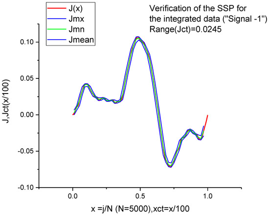
Figure 1.
This figure demonstrates the similarity of the integral curve obtained from the TLS corresponding to Signal 1. The initial curve contains N = 5000 data points, the compression parameter b = 100 and the range between compressed curves is 0.0245.
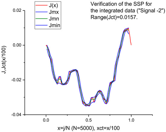
Figure 2.
This figure demonstrates the similarity of the integral curve obtained from the TLS corresponding to Signal 2. These compressed curves are obtained in the same conditions (N = 5000 data points, a compression parameter b = 100 and a range between compressed curves of 0.0157).
3.1. Description of Real Data
To verify the efficiency of the proposed algorithms, two sets of data were generated. The first, subsequently designated Signal 1, comes from the simulation of a first-order system with the transfer function
with a uniform noise as input. For the simulation, the sample time is chosen equal to Te = 0.624 ms. Thus, these data do not initially exhibit a power-law behavior.
Conversely, the second data set denoted Signal 2 was obtained under the same simulation conditions, but this time simulating a fractional system of the transfer function:
For the simulation, the transfer function is approximated by a 10 poles and zeros distribution [9,13]. Thus, these data do exhibit a power-law behavior.
3.2. Detection of the Hidden Self-Similarity
Here and below the measured data are denoted “Signal-1 (S1)” and “Signal-2 (S2)”, correspondingly. Each signal has approximately 8 × 10⁵ data points. Signal 1 is shown in Figure 3. How can the number of data points be reduced and the hidden self-similar behavior found? The desired algorithm can be divided into several successive steps. These steps are shown in an example of the processing of Signal 1.
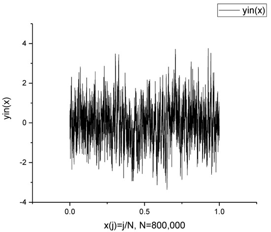
Figure 3.
The initial Signal 1 forms a trendless sequence with 8 × 10⁵ data points.
S1. The initial noise band/tape having Nb data points is transformed to a rectangle matrix having N rows (=5000) × M columns (=160) = Nb = 8 × 10⁵.
S2. Then for each column m having N rows, we find only three invariant points Yup(m) = max(m), Ymn(m) = mean(m) and Ydn(m) = min(m) that do not change their values relative to N! permutations in the fixed column. As the result of this action, we obtain three distributions over all the columns. They are shown in Figure 4. Then, in order to suppress the high-frequency fluctuations, we integrate these three distributions numerically by a trapezoid relative to its mean value
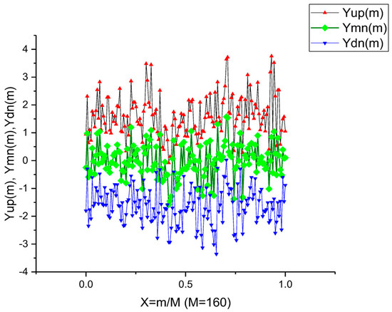
Figure 4.
Distribution of three functions Yup(m) = max(m), Ymn(m) = mean(m) and Ydn(m) = min(m) over all the columns (M = 160) that are obtained from the initial noise band depicted in Figure 3.
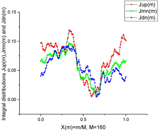
Figure 5.
Integral distributions that are obtained from the distributions depicted in Figure 4. The numerical integration plays the role of a specific filter helping to remove the high frequency fluctuations.
S3. Verification of the self-similarity principle. Integration of the initial trendless sequence depicted in Figure 3 with the help of expression (39) and comparison of this integral curve Jt(x) with the reduced integral curve Jmn(m). We should stress here again that the first curve contains 8 × 10⁵ data points, while the second one contains only 160 points coinciding with the number of columns. Their similarity is shown in Figure 6 for Signal S1.
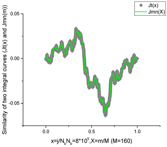
Figure 6.
This plot demonstrates the similarity of the integral curve Jt(x) obtained from the total number of data points 8 × 10⁵ (grey rhombs) and the integral curve (bolded green line) obtained from the curve Ymn(m).
It indicates that the three integral curves shown in the previous image are self-similar and are characterized by a linear combination of the power-law exponents.
S4. For fitting purposes, we use the functional Equation (9) that contains in solution (13) only two possible power-law terms and the term corresponding to the root r3 = 1. It is convenient to choose the normalized curve for all integral curves defined as
where the function Y(X) coincides with that of the integral curves Jup(X), Jmn(X) and Jdn(X).
S5. If the log-periodic corrections are removed from (13), we obtain the simplified function that enables the desired power-law exponents to be calculated
The approximate expression (41) can be transformed into the Euler equation
That makes it possible to find the desired roots by the EC method [14]. After that, one can find the decomposition coefficients before the log-periodic functions in (13) and, finally, achieve the desired fit of the integral curves Jup(X), Jmn(X) and Jdn(X). The functions prepared for the fitting procedure are shown in Figure 7. The minimum value of the relative error used for calculation of the optimal ln(ξ) is shown in Figure 8. The fit of the two functions ln(Jmn(X)) and Jmn(X) is shown in Figure 9. In Figure 10, we demonstrate the distributions of the coefficients that figure in solution (13).
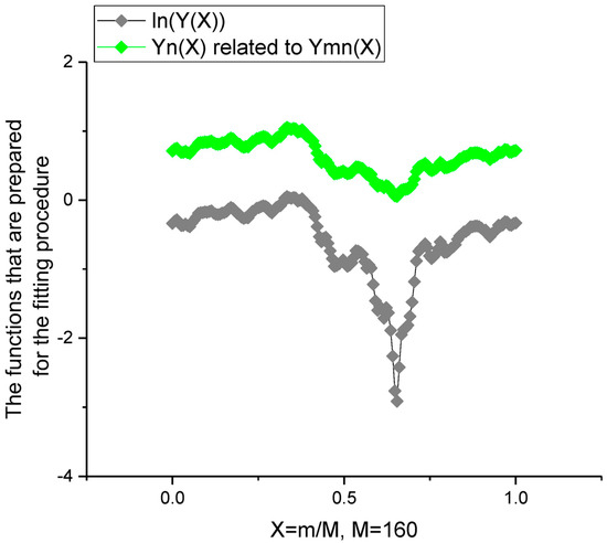
Figure 7.
These functions are prepared for the fitting procedure. Above we demonstrate the normalized Jmn(X) and below ln(Jmn(X))).
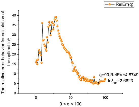
Figure 8.
The dependence of the relative error for calculation of the nonlinear parameter lnξ. For calculation of the lnξopt, expression (34) is used.
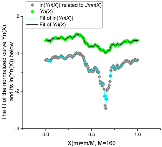
Figure 9.
The fit of the normalized curve Yn(X) corresponding to Jmn(X). The value of the relative error is given in Table 1.
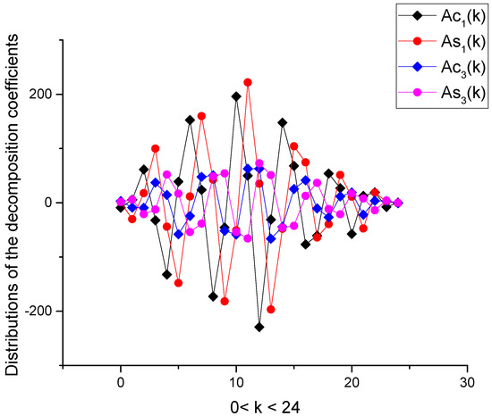
Figure 10.
Distribution of the decomposition coefficients that enter in the log-periodic functions in solution (13).
S6. If the calculated weights are normalized and satisfy condition (25), then the Bellman’s inequality is satisfied. In our case, it is expressed in the form (33). Figure 11 demonstrates the numerical verification of expression (43), relative to nonlinear parameter s that enters into expression (31)
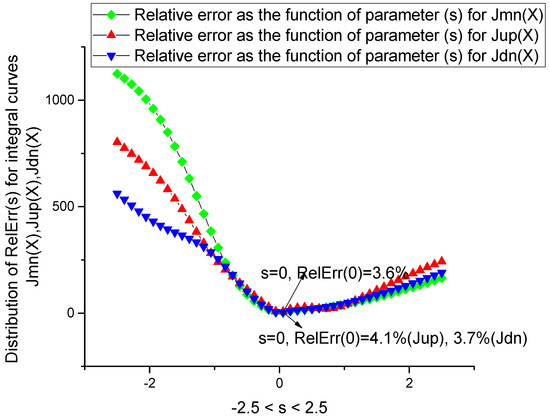
Figure 11.
Numerical verification of Bellman’s inequality (33) for all three functions: Jmn(X), Jup(X) and Jdn(X).
The additional fitting parameters for the normalized integral curve Jmn(X) are shown in Table 1. Explanation of the fitting procedure and detection of the power-law dependencies requires nine figures. Therefore, for the remaining two normalized integral curves Jup(X), Jdn(X), we show only the desired fitting parameters in Table 1. However, for Signal 2, we are forced to show some important figures for comparison with the processing procedure of Signal 1 shown above. Figure 12, Figure 13, Figure 14, Figure 15, Figure 16, Figure 17 and Figure 18 and their captions demonstrate the details of the processing procedure related to Signal 2. Again, we confirm the criterion of a “hidden” self-similarity associated with the compressed integral curves shown in Figure 1 and Figure 2 and Figure 6 and Figure 15 and show the accurate fit of the normalized function for Jmn(X) (Figure 16).

Table 1.
The set of the fitting parameters for the normalized integral curves for Signal 1.
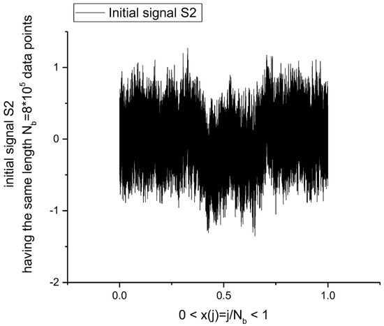
Figure 12.
The initial Signal 2 forms a quasi-trendless sequence with the same 8 × 10⁵ data points.
Figure 13.
Distribution of three functions Yup(m) = max(m), Ymn(m) = mean(m) and Ydn(m) = min(m) over all the columns (M = 160) that are obtained from the initial noise band S2 depicted in Figure 12. We note that the functions Yup(m), Ydn(m) repeat, approximately, the envelopes of the initial Signal 2.
Figure 14.
Integral distributions that are obtained from the distributions depicted in Figure 13. The numerical integration plays the role of a specific filter helping to remove the high frequency fluctuations and decreasing the number of the fitting parameters.
Figure 15.
This plot demonstrates the similarity of the integral curve Jt(x) obtained from the total number of data points 8 × 10⁵ (black balls) and the integral curve (bolded red line) obtained from the curve Ymn(m).
Figure 16.
The fit of the normalized curve Yn(X) corresponding to Jmn(X) The value of the relative error is given in Table 2.
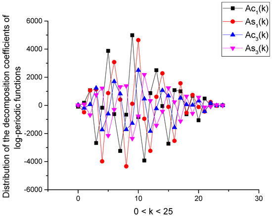
Figure 17.
Distribution of the decomposition coefficients in the log-periodic functions in solution (26).

Figure 18.
Numerical verification of Bellman’s inequality for all three functions Jmn(X), Jup(X) and Jdn(X) obtained for Signal 2.
To conclude this section, one can give the following “reading” of the SSP. Let us introduce the scaling operator as
Based on this operator, one can rewrite the basic SSP Equation (25) in the following form
where the decomposition coefficients in (25) (wl,) are related to the “roots” rl (l = 1, …, L) in (45) as
If the scaling operator’s link in Equation (44) is successful, Equation (45) immediately provides all the potential “scalings” that may be applied to the system under consideration. In our example, analysis of the integrated curves generated in various scales supports Equation (44) (see Figure 1, Figure 2, Figure 6 and Figure 15). As seen above, the generalized geometric mean defined by (32) finds the global fitting minimum in perfect compliance with inequality (33) if one of the roots in (46) coincides with the unit value.
Equation (45) admits the further generalization for the 3D case. In this case, one can define a more general scaling operator
Here F(z1,z2,z3) is an arbitrary given function. Equation (48) represents the most general case of the SSP for the 3D case.
It indicates that the three integral curves shown in the previous image are self-similar and are characterized by a linear combination of the power-law exponents.
One can note that in [15], a similar algorithm was applied to real acoustic data (sounds captured from “a wind” and these data are available at “soundspunos.com” site), demonstrating that the envelopes of these “noisy” data totally confirm the self-similarity principle and can be fitted by functions containing complex-conjugated power-law addings.
4. Results and Discussion
In this paper, we demonstrated how the self-similarity principle leads to a broad class of power-law dependencies. For linear circumstances, this concept is expressed by expression (25), whereas for nonlinear cases, it is expressed by expression (31). As a result, there are two categories into which all researchers studying fractional operators might be placed. In many common equations such as diffusion, Schrödinger, wave, etc., the majority of researchers start with mathematical generalizations of fractional integrals/derivatives and “swap” integer operators with non-integer ones, enabling them to obtain the necessary power-law dependencies as a result of this replacement. They acquire fresh power-law dependencies that must be contrasted with actual data.
The lack of a tangible meaning for such mechanical replacement is its weak point. A small portion of the research adopts a more skeptical approach and attempts to assess experimental data and connect empirical relationships with power-law exponents related to microscopic matter structure. This tendency is seen, for instance, in the mechanical relaxation of viscous materials [16] and dielectric spectroscopy [17]. A large number of studies merely ignore a group of functional equations that result in the desired power-law dependence. The suggested self-similarity concept in this study can be a reliable source of new power-law dependencies because it can be simply and regularly applied to numerous complicated systems, even in the most basic scenario
This functional Equation (50), as it is shown above, can be applied to many random curves with a clearly expressed trend. It has a solution
and contains the power-law dependencies with complex-conjugate exponents. Therefore, rather than replacing equations containing integer powers by fractional operators, perhaps it would be wise to pay closer attention to the SSP if we carefully evaluate the data that are described by power laws? One of us (RRN) would like to recall the building of the mesoscopic theory of percolation currents in electrochemistry, which was based on the derivation of a linear self-similar Equation (15) for L = 2 [18]. Taking into account the information on how to measure the spatial fractal dimensions provided in [19,20], it might be useful to start with the analysis of a self-similar dynamic process and discover a suitable fractal that corresponds to the required fractional integral in order to obtain the matching fractional integral or derivative. Finding a class of fractals that, for example, fulfills Equations (25) and (31) related to the self-similar principle, would be particularly intriguing. Some efforts were made in this direction in [21]. If such a general connection were found, then these modified fractals generated by SSP would give rise to a new class of fractional integrals. Instead of imposing replacement equations (without clearly justifying their physical significance) for the fitting of real data, this is a more natural technique to connect fractals with various versions of fractional integrals. We provide the following scheme to provide a deeper understanding of “the location” that distinguishes power-law models from fractional models. We provide the following scheme (Figure 19).
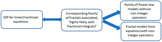
Figure 19.
This diagram clarifies the “location” of each block and the direction that appears in contemporary fractional calculus.
The SSP was founded on a dynamic/static fractal geometry model that results in the desired power-law behavior. To establish the origin of the observed power-law behavior with the fractal structure of the matter and likely with the fractional operator that can accurately describe the measured data, it would be desirable for any researcher to have the corresponding fractal model that exists in a mesoscale region.
Author Contributions
Writing—review & editing, R.R.N. and J.S. All authors have read and agreed to the published version of the manuscript.
Funding
This research received no external funding.
Data Availability Statement
The data can be available under the personal request of a potential reader.
Conflicts of Interest
The authors declare no conflict of interest.
Abbreviations
| CPE | constant-phase element |
| GGM | the generalized geometric mean |
| LLSM | linear least square method |
| TLS | trendless sequence |
| SSP | self-similar principle |
References
- Sabatier, J.; Farges, C.; Tartaglione, V. Fractional Behaviours Modelling. In Intelligent Systems, Control and Automation: Science and Engineering; Springer: Berlin/Heidelberg, Germany, 2022; Volume 101. [Google Scholar] [CrossRef]
- Sabatier, J. Modelling Fractional Behaviours without Fractional Models. Front. Control Eng. 2021, 2, 716110. [Google Scholar] [CrossRef]
- Tartaglione, V.; Farges, C.; Sabatier, J. Nonlinear dynamical modeling of adsorption and desorption processes with power-law kinetics: Application to CO2 capture. Phys. Rev. E 2020, 102, 052102. [Google Scholar] [CrossRef] [PubMed]
- Nigmatullin, R.; Machado, J.; Menezes, R. Self-similarity principle: The reduced description of randomness. Cent. Eur. J. Phys. 2013. [Google Scholar] [CrossRef]
- Beckenbach, E.F.; Bellman, R. Inequalities; Springer Science & Business Media: Berlin, Germany, 2012; Volume 30. [Google Scholar]
- Mandelbrot, B.B. The Fractal Geometry of Nature; W.H. Freeman: New York, NY, USA, 1982. [Google Scholar]
- Feder, J. Fractals; Plenum Press: New York, NY, USA; London, UK, 1988. [Google Scholar]
- Nigmatullin, R.R.; Vorobev, A.S. Discrete Geometrical Invariants: How to Differentiate the Pattern Sequences from the Tested Ones? In The Proceedings of the ICFDA19 Conference; Proceedings in Mathematics & Statistics; Springer: Singapore, 2019. [Google Scholar]
- Oustaloup, A.; Levron, F.; Mathieu, B.; Nanot, F.M. Frequency band complex noninteger differentiator: Characterization and synthesis, IEEE Transactions on Circuits and Systems. IEEE Fundam. Theory Appl. 2000, 47, 25–39. [Google Scholar]
- Gil’mutdinov, A.K.; Ushakov, P.A.; El-Khazali, R. Fractal Elements and Their Applications; Springer International Publishing: Cham, Switzerland, 2017. [Google Scholar]
- Raoul, R. Nigmatullin1 José Tenreiro Machado, Rui Menezes. Self-similarity principle: The reduced description of randomness. Cent. Eur. J. Phys. 2013, 11, 724–739. [Google Scholar]
- Nigmatullin, R.R.; Evdokimov, Y.K. The concept of fractal experiments: New possibilities in quantitative description of quasi-reproducible measurements. Chaos Solitons Fractals 2016, 91, 319–328. [Google Scholar] [CrossRef]
- Manabe, S. The non-integer integral and its application to control systems. ETJ Jpn. 1961, 6, 83–87. [Google Scholar]
- Nigmatullin, R. Recognition of nonextensive statistic distribution by the eigen-coordinates method. Phys. A 2000, 285, 547–565. [Google Scholar] [CrossRef]
- Raoul, R.; Nigmatullin, J. Sabatier How to detect and fit “fractal” curves, containing power-law exponents? Part 1 and 2. In Proceedings of the International Conference on Fractional Differentiation and its Applications (ICFDA 2023), Ajman, United Arab Emirates, 14–16 March 2023. [Google Scholar]
- Magin, R.L. Fractional Calculus in Bioengineering; Begell House Publishers, Inc.: Danbury, CT, USA, 2006. [Google Scholar]
- Jonscher, A.K. Universal Relaxation Law; Chelsea Dielectric Press Ltd.: London, UK, 1996. [Google Scholar]
- Nigmatullin, R.R.; Budnikov, H.C.; Sidelnikov, A.V. Mesoscopic theory of percolation currents associated with quantitative description of VAGs: Confirmation on real data. Chaos Solitons Fractals 2018, 106, 171–183. [Google Scholar] [CrossRef]
- He, C.H.; Liu, C. Fractal dimensions of a porous concrete and its effect on the concrete’s strength. Facta Univ. Ser. Mech. Eng. 2023. [Google Scholar]
- Yu, B.M. Comments on “Fractal Fragmentation, Soil Porosity, and Soil Water Properties: I. Theory”. Soil Sci. Soc. Am. J. 2007, 71, 632. [Google Scholar] [CrossRef]
- Nigmatullin, R.R.; Zhang, W.; Gubaidullin, I. Accurate relationships between fractals and fractional integrals: New approaches and Evaluations. Fract. Calc. Appl. Anal. 2017, 20, 1263–1280. [Google Scholar] [CrossRef]
Disclaimer/Publisher’s Note: The statements, opinions and data contained in all publications are solely those of the individual author(s) and contributor(s) and not of MDPI and/or the editor(s). MDPI and/or the editor(s) disclaim responsibility for any injury to people or property resulting from any ideas, methods, instructions or products referred to in the content. |
© 2023 by the authors. Licensee MDPI, Basel, Switzerland. This article is an open access article distributed under the terms and conditions of the Creative Commons Attribution (CC BY) license (https://creativecommons.org/licenses/by/4.0/).