Abstract
The presence of bruises on fruits often indicates cell damage, which can lead to a decrease in the ability of the peel to keep oxygen away from the fruits, and as a result, oxygen breaks down cell walls and membranes damaging fruit content. When chemicals in the fruit are oxidized by enzymes such as polyphenol oxidase, the chemical reaction produces an undesirable and apparent brown color effect, among others. Early detection of bruising prevents low-quality fruit from entering the consumer market. Hereupon, the present paper aims at early identification of bruised lemon fruits using 3D-convolutional neural networks (3D-CNN) via a local spectral-spatial hyperspectral imaging technique, which takes into account adjacent image pixel information in both the frequency (wavelength) and spatial domains of a 3D-tensor hyperspectral image of input lemon fruits. A total of 70 sound lemons were picked up from orchards. First, all fruits were labeled and the hyperspectral images (wavelength range 400–1100 nm) were captured as belonging to the healthy (unbruised) class (class label 0). Next, bruising was applied to each lemon by freefall. Then, the hyperspectral images of all bruised samples were captured in a time gap of 8 (class label 1) and 16 h (class label 2) after bruising was induced, thus resulting in a 3-class ternary classification problem. Four well-known 3D-CNN model namely ResNet, ShuffleNet, DenseNet, and MobileNet were used to classify bruised lemons in Python. Results revealed that the highest classification accuracy (90.47%) was obtained by the ResNet model, followed by DenseNet (85.71%), ShuffleNet (80.95%) and MobileNet (73.80%); all over the test set. ResNet model had larger parameter sizes, but it was proven to be trained faster than other models with fewer number of free parameters. ShuffleNet and MobileNet were easier to train and they needed less storage, but they could not achieve a classification error as low as the other two counterparts.
Keywords:
bruise; classification; 3D-CNN; fruit; hyperspectral imaging; lemon; machine learning; tensor imaging 1. Introduction
Lemon fruit is well-known for having soluble dietary fiber that helps in healthy digestion. More than half of the vitamin C needed by the body is provided using lemon consumption, which aids in strengthen the immune system and reduces the risk of heart disease and stroke [1,2]. The origins of lemon consumption probably date back to the south of China and it has been cultivated in Asia for more than 2500 years. Main lemon producer countries in the world are Spain, Mexico, the Netherlands, South Africa, and Turkey. It is desirable to use fresh lemons because they are flavorful and all parts of lemons can be used. For example, guaro drink is made from lemon juice or its peel is used as a seasoning in desserts. Processed lemons (dehydrated peel, citric acid, pomace, pectin and limonene) are used in the food and non-food industry. Lemon consumption is increasing in producing and non-producing countries around the globe. However, bruised fruit does not constitute a health hazard but it is displeasing in terms of visual appearance to consumers.
Post-harvest operations include a complex route from the garden to the market [3,4] which includes various operations such as harvesting, packaging, sorting, storage, and transportation. Although during these operations every effort is made not to damage the fruit, nevertheless often fruit suffers from mechanical damage caused by either dynamic or static load [5,6]. Lemon bruises are of great concern to the lemon industry and retailers because they reduce not only the visual appearance, but also the quality of the fruit and thus can cause significant economic losses. Bruising usually occurs in the tissue under the fruit peel cover. The amount of bruising depends on a number of factors such as the time of harvest, the maturity of the product, and the number of days after harvest. Physiological, biochemical and environmental properties are affected by the sensitivity of a given fruit to bruising [7].
Several studies, including hyperspectral imaging and near-infrared spectroscopy, have been reported for bruising detection [8,9,10,11]. These optical techniques detect and evaluate changes or differences in optical properties (i.e., reflection or transmission of light) between normal and bruised tissues. However, reflection and transmission are not intrinsic properties and their measurement often depends on the sensing configuration, lightning conditions and the type of sensor. For instance, by the integration of image processing and spectroscopy, a spatial map of spectral changes can be obtained which has promising applications in the field of agricultural products quality assessment [12,13,14].
Convolutional neural networks (CNNs) are being widely used in computer vision scientists because it is a type of deep learning (a part of the machine learning framework) for processing structured arrays of data, such as images. They are able to properly recognize patterns in the input image such as circles, lines, gradients and even faces of higher lever structures with great success. Another advantage of this kind of CCN networks is that, unlike previous computer vision algorithms, they do not need pre-processing, segmentation and feature extraction and can work directly on an original image, but taking care that overfitting to the training set is not present after training, since this would greatly limit the generalization capability of the neural network to properly classify unseen input samples belonging to the test set [15]. The inputs of CNN structure are directly the input images of interest to be automatically analyzed. CNNs have 1D, 2D and 3D types, among others. In 1D-CNN, the network moves in one direction. They are commonly used on time series data analysis. In 2D-CNNs, the kernels move in two spatial independent directions, and they are often used in image labeling and image processing (computer vision). 3D-CNN has a kernel that moves in three independent spatial directions. Those are used in 3D (volumetric) images of interest, such as MRI and CT body scans in the field of medicine.
Rivera [16] et al. studied on early detection of mango mechanical damage using machine learning and near infrared (NIR) hyperspectral images. The inner properties of healthy and damaged areas of mango were obtained in the range of 650–1100 nm and then further analyzed to select the most effective wavelengths for proper discrimination (classification). Results showed that the correct classification rate was 97.9% inside the three-day time gap after the damage was done. Following the study conducted by [17] on persimmon fruit to detect bruising using hyperspectral imaging in the range of 450–1040 nm, it is found that an algorithm based on principal component analysis (PCA) was able to identify healthy (90%) and damaged (90.8%) fruit at high correct classification rates. Also, they developed a model based on partial least squares discriminant analysis (PLS-DA) that was able to classify the fruits based the moment when bruising happened and thus the fruit classes corresponding to 0, 1, 2 and 3 days after bruising took place were discriminated with an overall mean accuracy of 99.4%. Che [18] et al. developed a pixel-based method to detect bruised area in apple fruit. Hyperspectral images of 60 apples were taken at time intervals of 0, 12, and 18 h after an artificial bruising process was conducted. After selecting the region of interest (ROI), different recognition models were developed. Results stated that the random forest (RF) model had the highest correct classification rate (99.9%). Fan [19] et al. developed a bruise detection system for blueberry fruit using a near-infrared (NIR) hyperspectral (950–1650 nm) system. They captured images at 30 min, 2 h, 6 h, and 12 h intervals after mechanical impact on blueberries had happened. A least squares support vector machine (LS-SVM) based model was developed to compute the distribution of spatial bruising. The overall classification accuracy for 30 min, 2 h, 6 h, and 12 h gaps was 77.5%, 83.8%, 92.5% and 95.0%, respectively. Li [20] et al., captured hyperspectral images of peaches at 12, 24, 36, and 48 h after impact. To create a discrimination model, the spectrum and properties of the samples were extracted. The results showed that according to the PLS-DA algorithm, the correct classification rates were 96.67%, 96.67%, 93.33% and 83.33% for 12, 24, 36 and 48 h, respectively.
Zheng et al. [21] proposed a classifier to separate healthy and bruised pear. A thermal imaging system at the ranges of 8–14μm was used to capture images. The thermal images were analyzed by the gray-level co-occurrence matrix. A total of 3246 and 1125 samples were used as training and test data set, respectively. The best test prediction accuracy obtained was 99.25%. Gai et al. [22] conducted a study based on 1D-convolutional neural network integrated with hyperspectral images to detect apple bruises. The number of 20 wavelengths were determined to proper identification. The accuracy of system was 95.79% on the test set.
Scientists believe that up to 35% of bruises occur during harvesting and transportation [23]. In order to minimize post-harvest losses, proper management, transportation, and storage techniques are needed. The bruised fruit does not only cause a decrease in marketable value, but also during the storage period, it is susceptible to various diseases due to peel/tissue damage and to the watery nature of the bruised tissue, thus making it necessary to separate bruised fruits from healthy (sound, undamaged) ones.
Application of convolutional neural networks on images is widely used and proven to achieve state-of-the-art performance on image tasks like classification, object detection, noise reduction, etc. CNNs help in extracting information from different channels of input images (3 channels in the case of RGB) by considering the spatial relation of pixels and providing encoding features from the image.
As it can be inferred from the literature review, studies on this field and topic can be divided into two categories: first category are those conducted on bruise detection after a few days (long period of time). In this case, the fruit piece is discolored and high accuracy will be obtained to distinguish between sound and bruised fruits. The second category are those conducted on fruits such as apples which will discolor in a rather short period of time, so it can be expected that the healthy and bruised samples will be classified with high accuracy only after a short period of time has passed from damage instant. Present paper deals on early identification of bruised lemons using 3D convolutional neural networks. Lemon is one of the fruits in which the visible symptoms of bruising appear at a later phase. Our methodology concatenates different spectra and create a 3D tensor image for each sample in input dataset. This can represent a 3D (volumetric) image similar to a human body medical imaging systems output. Furthermore, the 3D -NN layers are used to extract information from this 3D tensor image by considering the spatial information of the pixels in all three spatial dimensions. As a result, the relation of pixels in a single spectrum and its adjacent spectra values (similar wavelengths), as well as the near (local) spatial neighbor pixels in different spectrums, are considered while in the image encoding process of the CNN layers. Consequently, both local spectra and local spatial relevant information of different spectrums and spatial points, are considered and taken into account simultaneously in the final out classification decision of the automatic machine learning classification models here introduced.
2. Materials and Methods
An illustration of classification task workflow is given in Figure 1. The dataset contains only 210 images in 3-dimensions. Some images were corrupted or do not have enough spectrum signatures similar to the average. Next, all the samples were resized to (f,x,y) = (174,160,120) hyperspectral 3D tensor images size, for frequency bands (f wavelengths, frequency resolution), and x-axis and y-axis spatial coordinate system, with above mentioned frequency (wavelength bands) and space resolution (pixel) values, respectively. To overcome the small sample size of the dataset, data augmentation techniques were applied to increase the dataset size.
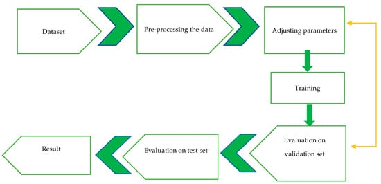
Figure 1.
An illustration of our machine learning framework classification task workflow.
2.1. Collecting the Samples
A total of 70 healthy and intact lemons were obtained from orchards. In order to avoid bruising during transport from the garden to laboratory, the fruits were protected inside the covers. First, all fruit was labeled and the hyperspectral images of all were captured as the healthy class (class label 0). Next all lemons were drop from a height of 30 cm hitting the ground producing artificial bruising. Then, the hyperspectral images of all bruised samples were captured at 8 (class label 1) and 16 h (class label 2) after bruising.
2.2. Hardware System for Data Collection
A hyperspectral camera with software and built-in scanner (Noor Imen Tajhiz Co.; https://hyperspectralimaging.ir/, accessed on 2 February 2023, made in Iran-Kashan) were used. The spectral range of the camera was 400 to 1100 nm and its spectral resolution was 2.5 nm. The type of camera scan was angular scan and the accuracy of spatial resolution for an object at a distance of 1 m was equal to 250 microns. In order to avoid ambient light noise, a chamber was used with artificial illumination by 2 lamps placed opposite to each other (20 W), c.f. Figure 2. To prevent the brightness of the sample, the light should not directly illuminate the sample, but it should be installed in such a way that it illuminates the space inside the chamber uniformly.
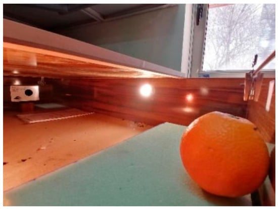
Figure 2.
Setup of proposed hardware system to perform input samples hyperspectral imaging.
2.3. Removal of the Noisy Spectral Data
Images captured by the hyperspectral camera were at the range of 400–1100 nm. Due to various reasons such as ambient noise, light effect and others, the beginning and the end of the spectrum range were highly noisy. Therefore, those noisy frequency bands data were discarded since they did not provide useful information (see a number of hyperspectral image examples in Figure 3. At the end, a total of 174 spectral images where picked from each individual input fruit sample, at a range of 550–900 nm and selected to be further analyzed.
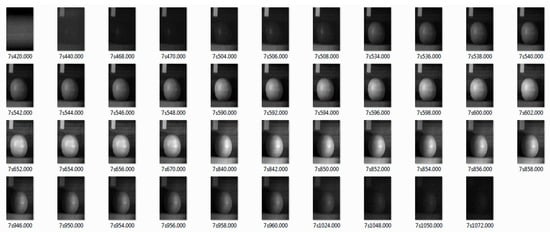
Figure 3.
Some examples of hyperspectral images at the wavelength range of 400–1100 nm: as is apparent from images, both initial and final frequency bands were considered irrelevant and thus discarded.
2.4. The 3-Dimensional (3D) Structure of the Hyperspectral Imaging Fruit Samples
Figure 4 shows an example of a lemon input tensor 3D hyperspectral image. After preprocessing, there are 174 spectrums for each sample data, and each spectrum has 160 by 120 spatial pixels (19,200 pixels). The example below shows the spectrum of a lemon training sample tensor image.
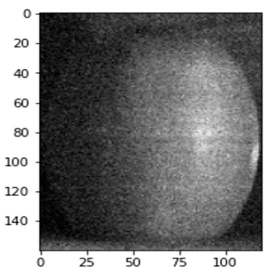
Figure 4.
A sample tensor 3D hyperspectral image at a particular fixed spectrum frequency band: dataset consisted of 174 wavelength band images like the one here depicted, with a spectral resolution of 2.5 nm between frequency bands inside (550–900 nm) wavelength range, and (160 × 120) spatial resolution pixels, totaling 19,200 spatial pixels in each spectral band image.
2.5. 3D-Convolutional Neural Network Classifiers
Convolutional Neural Networks (CNN) are a special type of Neural Networks designed for detecting image-specific features and patterns from pixels inside the image. As illustrated in Figure 5, given an input image that may contain multiple channels (3 channels in the case of RGB images), CNN encodes image-specific features required for making inferences on inputs in image tasks. This encoding is done using fixed-sized kernels ‘walking’ (convolution) through the whole image space. As a result, usage of CNN provides a state-of-the-art method for tasks like image classifications, object detection, image reconstruction, etc.
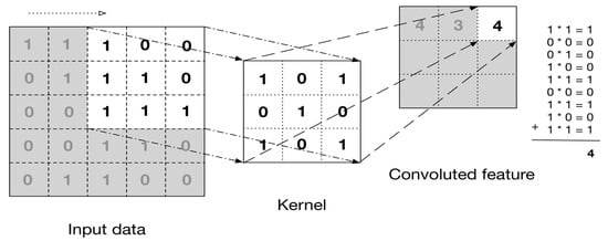
Figure 5.
Convolutional Neural Networks (CNN) layer with a kernel size 3 and its generated encoded output after convolution.
A convolutional layer with kernel k and image matrix can be formalized as Equation (1) [24]:
where x is image matrix, T stands for vector transpose, z is the feature value (i,j) of layer l and the kernel k of the output feature matrix and ω and b are weight vector and bias matrix of kernel k and layer l, respectively.
The most important limitation of Artificial Neural Network (ANN) is their complexity and efficiency when dealing with high-dimensional inputs like image pixels. If each input is represented by a 64 × 64 pixel image, the number of weights needed by a neuron in the first layer would be 12,288 [24]. This makes CNN a suitable choice for image tasks.
In an image classification task, a model can use CNN layers to extract spatial information from images and generate encoded feature matrices (feature extraction). After some layers of CNN, it will use fully connected neural network layers to provide a predicted label given these encoded features (classification). This process is illustrated in Figure 6 [25].

Figure 6.
An example of an image classification by a CNN network architecture.
At the present paper, 3D-CNN network was leveraged so that it accepts 3D images as inputs. The input tensor to this network has 4 dimensions, including the number of channels (Figure 7) [26].
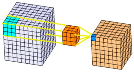
Figure 7.
Example of a 3D-CNN with a 3D kernel depicted as an orange box.
Different 3D-CNN models such as ResNet, ShuffleNet, DenseNet, and MobileNet at the PyThon programing framework, were used to predict the output class labels, as detailed next.
2.5.1. ResNet Architecture
Using deep networks introduces several problems in the training phase, like the degradation problem that causes the model to be harder to train and reduces the output classification accuracy of the model. ResNet model solves this problem by defining residual connections. This helps define deep networks without those optimization problems and still have a model which could easily be trained and maintain its high output accuracy [27]. The building block of this model is represented in Figure 8. These connections enhance the gradient flow in backpropagation and prevent degradation problems like gradient vanishing.
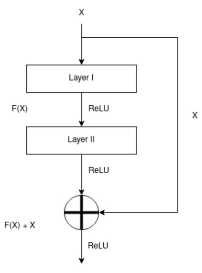
Figure 8.
Example of Residual Connections in the building block of ResNet architecture.
2.5.2. ShuffleNet Architecture
ShuffleNet is an extremely efficient network that uses Pointwise Group Convolution and Channel Shuffle to achieve an efficient performance for environments with limited available resources [28]. An example of ShuffleNet building block is illustrated in Figure 9.
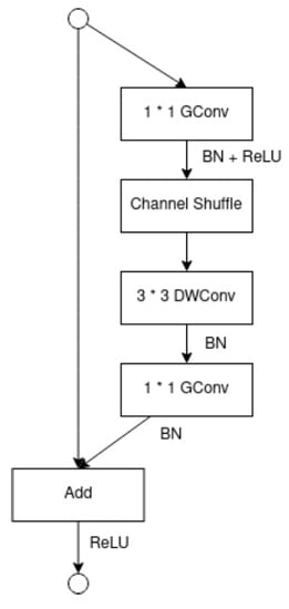
Figure 9.
Building block of ShuffleNet depicted with Channel Shuffle and Pointwise Group Convolution in it.
2.5.3. DenseNet Architecture
In the DenseNet network, each layer is connected to every other preceding layer. This helps in preventing the vanishing gradient problem and also strengthens feature propagation [29]. Figure 10 illustrates the building blocks of DenseNet also known as Dense Blocks. Additionally, DenseNet helps in using fewer parameters in the learning process. Leveraging the knowledge of previous layers also reduces the redundancy in the learned feature maps.
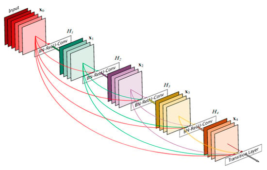
Figure 10.
Example of Dense Blocks depicted in DenseNet architecture.
2.5.4. MobileNet Architecture
Similar to ShuffleNet, MobileNet introduces a new architecture to efficiently learn on embedded and mobile applications with limited resources available [30]. It uses depth-wise separable convolutions that reduce the number of parameters compared to simple CNN networks. A depth-wise separable convolution is illustrated in Figure 11 containing Depthwise convolution and Pointwise convolution layers.
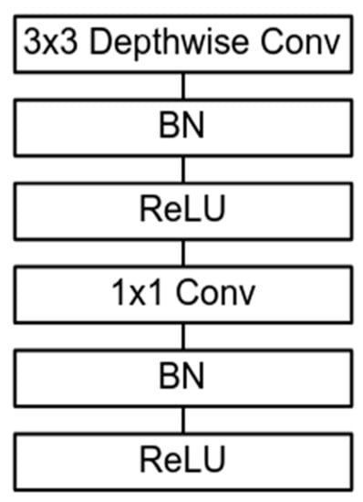
Figure 11.
Building block of MobileNet containing Depthwise Convolution and Pointwise Convolution boxes.
2.6. Train, Test and Validation Disjoint Sets: A Partition of the Input Dataset
The input image hyperspectral dataset is split into the disjoint train, test, and validation sets with portions of 70%, 10%, and 20% of the total, respectively. The number of samples in the dataset for each label (class) is as follows (before augmentation), see Table 1.

Table 1.
Number (#) of samples in the dataset and in train/test/validation disjoint sets.
3. Results
3.1. 3D-CNN Model Parameter, NN Size and Training Time
Multiple CNN models (3D versions), ResNet, ShuffleNet, MobileNet, and DenseNet, were used. They had different training times and parameter sizes (See Table 2).

Table 2.
3D-CNN model parameter sizes and training time per epoch.
The ShuffleNet model [28] uses Channel Shuffle Operation and Pointwise Group Convolution to be highly efficient. As a result, it consumes less amount of resources, less computational load and it can be trained faster with less memory usage in comparison to other models, like DenseNet. DenseNet uses Dense Blocks that help each layer collect the knowledge from all preceding layers [29]. ResNet model uses Residual Connections between its layers [27]. This enhances the training time as the gradient flow would be highly optimized. As a result, a deeper ResNet model with a larger parameter size has a faster training time in comparison with the DenseNet model. MobileNet is also used for embedded applications where there is a limited computational power. It uses depth-wise separable convolutions to reduce the model size and at the same time make it more efficient.
3.2. The Final Deep Network Classifiers Structure
The batch size was 4 and also they were accumulated 2 epochs before one step in optimization (resulting in an effective batch size of 8). The well-known CrossEntropyLoss loss (error) function was used as the optimization criterion. In addition, the Adadelta optimizer with an exponential learning rate was applied that helped in achieving faster convergence and increased stochastic nature of the training process. It was started with a learning rate of 0.1 and was then reduced exponentially by a gamma factor of 0.95.
In order to use all the spatial information of the hyperspectral images, we concatenated the spectrums of each sample and created a 3D image. As a result, the input to our models is an image of size 174 × 160 × 120 pixels. One important hyper-parameter for our classifier in the training phase is the batch size. We had some limitations in the GPU memory storage (Google Colab. Environment). Additionally, the 3D-CNN models consume more memory storage space than 2D-CNN models because of the larger trainable parameters in these 3D model kernels and pooling layers. In order to overcome this limitation, we used a batch size of 4 with a gradient accumulation of two back propagations. This provides an effective batch size of 8 in our training phase, as already mentioned.
We used CrossEntropyLoss cost function to compute the error of the models. The last layer of the classifier uses a Softmax layer to provide a prediction probability for each of the classes. By using the cross-entropy loss, these logits (probabilities) are compared with the expected label vector which is a one-hot vector with one single non-zero value on the index of the expected label and zero on all other indices of the vector. As a result, if an error is introduced on these logits, it will go back to update model parameters through the backpropagation learning algorithm.
As the training optimizer, we used Adadelta [31]. Adadelta adapts the learning rate dynamically over time and has two major benefits: there is no need to manually select a global learning rate and addresses the problem of the continual decay of learning rates throughout training. We used an exponential scheduler for our optimizer and it helped the mode to faster converge to an optimal point in the loss function. We started with a base value of 0.1 for the learning rate and after each training epoch, this learning rate is multiplied by a gamma value of 0.95. The learning rate for epoch number n (n ≥ 1) can be calculated from initial learning rate easily using the following formula:
Using larger gamma values (0.95 to 0.99) results in high learning rates in the first 100 epochs which in turn results in larger gradient steps that reduce the training robustness of the model. Using small values of gamma increases the training time as well as reduces the chance to escape a local optimum in the loss function. As a result, it will take longer to reach high classification accuracy values.
3.3. The Behavior and Performance of All Four Deep Learning Classifiers after the Training Phase: Cross Entropy (CE) Loss Function and Output Classification Accuracy (%)
Figure 12 illustrates the behavior of the classifiers after the training phase. As shown, the DenseNet model has many oscillations in both the training and validation phase losses. In addition, the DenseNet model is a complex model which needs much more time and epoch numbers to train to achieve an accuracy equivalent to the ResNet case.
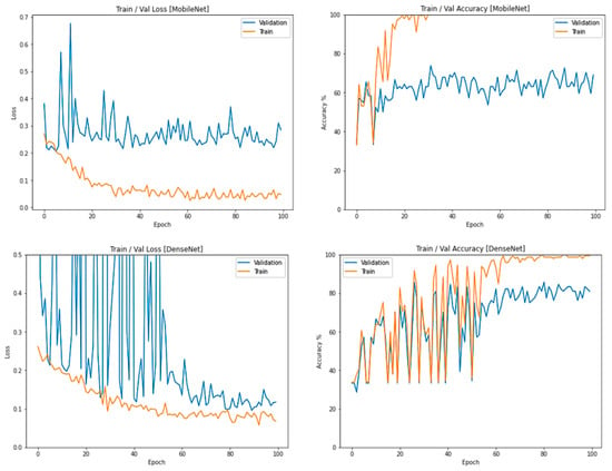
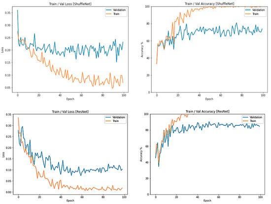
Figure 12.
Train (solid orange) and validation (solid blue) cross-entropy (CE) loss and classification accuracy (%) examples, after 100 epochs: ResNet, DenseNet, ShuffleNet, MobileNet.
The MobileNet model converges after 40 epochs and there was no noticeable further improvement in the validation loss after that epoch. This shows us that the 3D version of MobileNet does not have a high generalization power or in other words, this model can easily overfit to our small training dataset.
ShuffleNet is almost as efficient as MobileNet as illustrated in Table 2 in terms of both the training time and parameter set size. In contrast, it achieves higher accuracy on the training set, as compared to MobileNet. The reduction of training loss in the ShuffleNet is smoother and more robust than MobileNet and it converges after 60 epochs. As a result, there is an even higher chance to improve the accuracy of this model by increasing the training time.
None of the DenseNet and MobileNet models could achieve a lower loss on the training set when compared to ResNet. This shows us the power of ResNet models in reaching high accuracy in a limited amount of time and limited resources.
Both ShuffleNet and MobileNet use special structures to create an efficient model for embedded applications. Although they are easier and faster to train, we can see that there is a tradeoff for their generalization capability to the validation set in these two cases, since none of them can achieve a high classification accuracy, contrary to what DenseNet and ResNet models were able to do, over the validation set.
The ResNet model achieves lower loss in the training set as compared to all other models. This tells us that the residual connections in this model and using larger depths provide us with a highly generalizable model that can perform well on both the training and validation sets. None of the other models achieved a training loss of less than 0.05.
3.4. ResNet Lemon Bruising Classifier Results: Confusion Matrix and Precision-Recall Curves
In this section and the following ones, we evaluate the classifiers’ performance using their confusion matrix and the precision-recall curve on the test data. The confusion matrix illustrates the predicted labels of the model over the test data for each class. The element in the i’th row and j’th column of this matrix shows the number of samples in i’th class that are mis-classified as the j’th class by the model, over the test set.
The precision-recall curve (pr-curve) is a way of representing the behavior of a binary classifier. It is most useful whenever the classes sample are imbalanced (number of samples of one class clearly dominant over the others). The Average Precision (AP) summarizes such a plot as the weighted mean of precisions achieved at each output detection threshold, with the increase in recall from the previous threshold used as the weight. For a multi-class classifier, this curve can be plotted for each class C by considering other classes as a new class different from C (binarized problem, one class versus the remainder). Then AP can be calculated by micro-averaging on all classes.
The confusion matrix of the ResNet classifier is illustrated in Table 3. The large values on the diagonal of this matrix show that most of the predictions of this model on the test dataset were correct. The hardest label for this model was Class 2 because as we can see 2 of the samples were wrongly predicted out of all 7 samples for this class. This might be due to a problem in the test dataset since the number of misclassifications is small compared to other values. This model achieves an Average Precision of 0.95. We can see the AP for this model per class in Figure 13. The best average precision is for Class 1 which is 0.99. This means that it is easier for the model to classify Class 1 and distinguish it from all other classes. In contrast, finding the difference and distinguishing Class 0 from other classes is harder. This was shown in the confusion matrix too, where we can see that there are both Class 1 and Class 2 samples that are misclassified as Class 0.

Table 3.
Confusion matrix for ResNet (test set). Class 0, 1 and 2 refer to healthy, 8 and 16 h after induction of bruising, respectively.
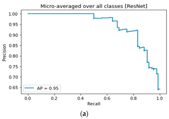
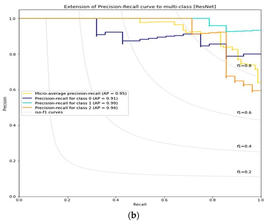
Figure 13.
Precision-Recall curve for ResNet model. (a): for the trained model, (b): for model separated by each class.
3.5. DenseNet Lemon Bruising Classifier Results: Confusion Matrix and Precision-Recall Curves
Table 4 shows the confusion matrix for DenseNet classifier. This classifier predicts all Class 1 samples correctly but has difficulties in classifying Class 0 and Class 2 objects. There are samples from Class 0 and Class 2 which are misclassified as other classes. The Average Precision for this model is 0.91 which is less than that of ResNet model (AP = 0.95).

Table 4.
Confusion matrix for DenseNet (test set): Class 0, 1 and 2 refer to healthy, 8 and 16 h after induction of bruising, respectively.
As a result, this model does not have the accuracy and power of ResNet model. We can check the precision-recall curve of this model in Figure 14. The best distinguishable class for this model is Class 1, similar to ResNet model, but Class 2 and Class 0 are harder to distinguish. In contrast to the ResNet model, DenseNet can distinguish Class 0 better than Class 2. This tells us that there are different encoded features considered by these two models in the classification layers.
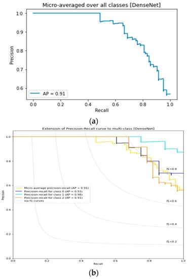
Figure 14.
Precision-Recall curve for DenseNet model. (a): for the trained model, (b): for model separated by each class.
3.6. ShuffleNet Lemon Bruising Classifier Results: Confusion Matrix and Precision-Recall Curves
The confusion matrix for ShuffleNet model is shown in Table 5. Similar to DenseNet, this model has no difficulty in predicting the correct labels of Class 1 samples in the test set. In contrast, ShuffleNet cannot predict Class 2 samples correctly and most of them are misclassified as Class 1. The ShuffleNet model has an Average Precision of 0.73. Compared two ResNet and DenseNet, this average precision is low and this tells us about the low generalization power of ShuffleNet model which could also be concluded from its confusion matrix. The precision-recall curve of ShuffleNet is plotted in Figure 15. By checking this curve, we conclude that this model can distinguish Class 1 better than all other classes but has problems with discriminanting Class 0 and Class 2.

Table 5.
Confusion matrix for ShuffleNet (test set): Class 0, 1 and 2 refer to healthy, 8 and 16 h after induction of bruising, respectively.
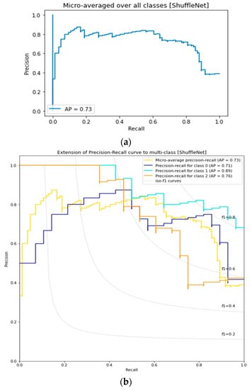
Figure 15.
Precision-Recall curve for ShuffleNet model. (a): for the trained model, (b): for model separated by each class.
3.7. MobileNet Lemon Bruising Classifier Results: Confusion Matrix and Precision-Recall Curves
The confusion matrix for MobileNet model is shown in Table 6. This model cannot predict Class 2 as it is shown inside this matrix. Most of these samples are misclassified as Class 0 or Class 1 and the model is only an expert in classifying Class 1 samples. The Average Precision for this model is 0.75. It is a little better than the ShuffleNet model but still far behind from those in ResNet and MobileNet. This tells us about the sacrifice (tradeoff) of generalization power for efficiency in the MobileNet model. As it is shown in Figure 16, this model cannot distinguish the Class 2 samples correctly.

Table 6.
Confusion matrix for MobileNet (test set): Class 0, 1 and 2 refer to healthy, 8 and 16 h after induction of bruising, respectively.
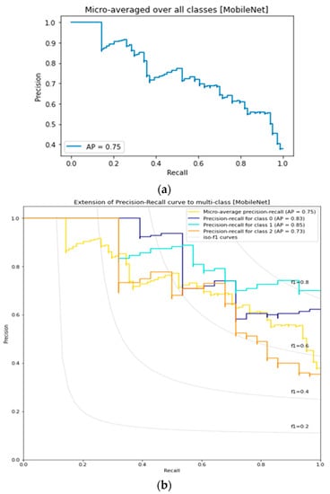
Figure 16.
Precision-Recall curve for MobileNet model. (a): for the trained model, (b): for model separated by each class.
By checking all these four precision-recall curves, we can also conclude that the most difficult class of lemon hyperspectral images is Class 2, as most of the models cannot distinguish them from other samples. In contrast, Class 1 samples are easier to distinguish. They can be distinguished easier even with human eyes but the difference between Class 2 and other classes is not easily determined. Finally, the ResNet model has the best generalization capability and Average Precision either on each class or overall.
3.8. Comparison of Lemon Bruising Classification Performance over the Four Deep Learning Architectures Considered: Accuracy (%), F1-Score, and AP
The overall results of these models are presented in Table 7, including the classification Accuracy, F1-score [32,33,34], area under the ROC curve (AROC), and the calculated AP per each label as well as the micro-averaged AP, computed over all three lemon classes. Figure 17 shows the classification Receiver Operation Characteristic (ROC) curves. These ROC curves illustrate the performance of each classifier by considering various threshold settings for each label versus the others. Consequently, it measures the success of the model in distinguishing each class from other two classes in a ternary classification.

Table 7.
Results of deep learning models evaluation comparison by their classification accuracy (%), F1-score, Average Precision (AP) and Area under the ROC curve (AROC): ResNet, DenseNet, ShuffleNet, and MobileNet.
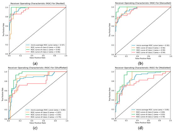
Figure 17.
Receiver Operation Characteristic (ROC) curve for each model (Micro averaged on all classes and for each class): (a) ResNet, (b) DenseNet, (c) ShuffleNet, and (d) MobileNet.
Based on the results, it is shown that the best accuracy is achieved by leveraging residual connections in the neural network, i.e., using ResNet. Although this model has larger parameter sizes, it can be trained faster rather than other models with fewer parameters. For instance, ResNet takes only 24 s in each training iteration, while DenseNet takes more than 40 s with number of parameters less than half of those in ResNet. This shows us that using the Residual Connections helps us achieve larger models in case of their generalization power and parameter size but still has better accuracy compared to the DenseNet model which takes longer to train and has also less robustness in the training phase.
As it has been seen, when using 3D-CNN layers in the models, it could be more difficult to train compared to standard CNN baseline models for 2D images. In addition, 3D-CNN models consume larger values of GPU memory because of larger parameters size and their training complexities. Thus, smaller batch sizes were used to overcome this limitation. Using smaller batch sizes alongside the difficulty of training 3D-CNN models results in lower accuracy for architectures with complex training paths like DenseNet. Similarly, this results in higher accuracy for the models that overcome this difficulty by leveraging Residual Connections.
Finally, some models are trying to leverage different techniques like Channel Shuffle Operation and Pointwise Group Convolution [35,36] to provide highly efficient models which could be used on embedded environments, like ShuffleNet and MobileNet. In contrast, these models sacrifice their generalization capacity power. Although they were easier to train and less storage is required for them, they could not achieve a lower loss, not even on the training set.
4. Conclusions
In this paper, four 3D-CNN model architectures were used to predict and classify lemon hyperspectral images in search of their freshness (bruises). The most important results obtained in this study are summarized next to conclude:
- The input dataset was small and the use of specific augmentations helped in generalizing the model’s prediction. Thus, we used two kind of data augmentation in this work: RandomHorizontalFlip and Color Jitter.
- There were limitations in the case of GPU memory resources and they were solved by accumulating gradients of smaller batches. With this method, we were able to train the networks with batch size 8, which is useful in the training phase.
- Using 3D-CNN layers helps us extract useful information from the 3D structure of concatenated hyperspectral images and leverage the spatial information within nearby pixels of the images and spectrums, thus having a double spectral-spatial classification.
- The best result is achieved from models with Residual Connections such as ResNet. These connections enhance the flow of gradients in these models. As a result, the model can be deeper without suffering the degradation problems like vanishing gradients and deeper models provide higher generalization power.
- Using exponential schedulers instead of a fixed learning rate helps to dynamically adapt the learning rate based on the epoch number. Furthermore, this scheduler enhances the process of finding an optimal point on our loss function by using big steps at the start of training and reducing the step sizes as we converge in the following epochs.
- Changing the architecture of the models in order to make them more efficient, like ShuffleNet and MobileNet, will sacrifice their performance and generalization power in complex tasks like 3D-CNN classifications in favor of their simplicity.
- The easiest label to distinguish in our dataset is Class 1 (8 h after bruising). Both Class 0 (healthy, un-bruised) and Class 2 (16 h after bruising) labels are harder to distinguish and need more powerful networks like ResNet and DenseNet to be correctly classified.
Author Contributions
Conceptualization, R.P.; methodology, S.S. and M.H.R.; software, M.D.; validation, S.S. and M.H.R.; formal analysis, R.P. and S.S.; investigation, R.P.; writing—original draft preparation, R.P.; writing—review and editing, J.I.A.; visualization, S.S.; supervision, M.H.R.; project administration, R.P. and S.S.; funding acquisition, R.P. and S.S. All authors have read and agreed to the published version of the manuscript.
Funding
This research received no external funding.
Data Availability Statement
Data is unavailable due to privacy or ethical restrictions.
Conflicts of Interest
The authors declare no conflict of interest. The funders had no role in the design of the study; in the collection, analyses, or interpretation of data; in the writing of the manuscript; or in the decision to publish the results.
References
- Rico, D.; Martin-Diana, A.B.; Barat, J.; Barry-Ryan, C. Extending and measuring the quality of fresh-cut fruit and vegetables: A review. Trends Food Sci. Technol. 2007, 18, 373–386. [Google Scholar] [CrossRef]
- Gulsen, O.; Roose, M.L. Lemons: Diversity and relationships with selected Citrus genotypes as measured with nuclear genome markers. J. Am. Soc. Hortic. Sci. 2001, 126, 309–317. [Google Scholar] [CrossRef]
- Issa, I.M.; Munishi, E.J.; Mubarack, K. Post-harvest Losses for Urban Fresh Fruits and Vegetables along the Continuum of Supply Chain Functions: Evidence from Dar es Salaam City-Tanzania. Can. Soc. Sci. 2021, 17, 75–87. [Google Scholar]
- Firdous, N. Post-harvest losses in different fresh produces and vegetables in Pakistan with particular focus on tomatoes. J. Hortic. Postharvest Res. 2021, 4, 71–86. [Google Scholar]
- Li, Z.; Thomas, C. Quantitative evaluation of mechanical damage to fresh fruits. Trends Food Sci. Technol. 2014, 35, 138–150. [Google Scholar] [CrossRef]
- Stropek, Z.; Gołacki, K. A new method for measuring impact related bruises in fruits. Postharvest Biol. Technol. 2015, 110, 131–139. [Google Scholar] [CrossRef]
- Hussein, Z.; Fawole, O.A.; Opara, U.L. Harvest and postharvest factors affecting bruise damage of fresh fruits. Hortic. Plant J. 2020, 6, 1–13. [Google Scholar] [CrossRef]
- Zhou, X.; Ampatzidis, Y.; Lee, W.S.; Zhou, C.; Agehara, S.; Schueller, J.K. Deep learning-based postharvest strawberry bruise detection under UV and incandescent light. Comput. Electron. Agric. 2022, 202, 107389. [Google Scholar] [CrossRef]
- Yin, H.; Li, B.; Zhang, F.; Su, C.-T.; Ou-Yang, A.-G. Detection of early bruises on loquat using hyperspectral imaging technology coupled with band ratio and improved Otsu method. Spectrochim. Acta Part A Mol. Biomol. Spectrosc. 2022, 283, 121775. [Google Scholar] [CrossRef]
- Guo, W.; Gao, M.; Cheng, J.; Zhou, Y.; Zhu, X. Effect of mechanical bruises on optical properties of mature peaches in the near-infrared wavelength range. Biosyst. Eng. 2021, 211, 114–124. [Google Scholar] [CrossRef]
- Huang, X.; Meng, Q.; Wu, Z.; He, F.; Tian, P.; Lin, J.; Zhu, H.; Zhou, X.; Huang, Y. Detection of early bruises in Gongcheng persimmon using hyperspectral imaging. Infrared Phys. Technol. 2022, 125, 104316. [Google Scholar] [CrossRef]
- Pourdarbani, R.; Sabzi, S.; Kalantari, D.; Paliwal, J.; Benmouna, B.; García-Mateos, G.; Molina-Martínez, J.M. Estimation of different ripening stages of Fuji apples using image processing and spectroscopy based on the majority voting method. Comput. Electron. Agric. 2020, 176, 105643. [Google Scholar] [CrossRef]
- Sabzi, S.; Pourdarbani, R.; Rohban, M.H.; García-Mateos, G.; Paliwal, J.; Molina-Martínez, J.M. Early detection of excess nitrogen consumption in cucumber plants using hyperspectral imaging based on hybrid neural networks and the imperialist competitive algorithm. Agronomy 2021, 11, 575. [Google Scholar] [CrossRef]
- Wieme, J.; Mollazade, K.; Malounas, I.; Zude-Sasse, M.; Zhao, M.; Gowen, A.; Argyropoulos, D.; Fountas, S.; Van Beek, J. Application of hyperspectral imaging systems and artificial intelligence for quality assessment of fruit, vegetables and mushrooms: A review. Biosyst. Eng. 2022, 222, 156–176. [Google Scholar] [CrossRef]
- Benmouna, B.; Pourdarbani, R.; Sabzi, S.; Fernandez-Beltran, R.; García-Mateos, G.; Molina-Martínez, J.M. Comparison of Classic Classifiers, Metaheuristic Algorithms and Convolutional Neural Networks in Hyperspectral Classification of Nitrogen Treatment in Tomato Leaves. Remote Sens. 2022, 14, 6366. [Google Scholar] [CrossRef]
- Rivera, N.V.; Gómez-Sanchis, J.; Chanona-Pérez, J.; Carrasco, J.J.; Millán-Giraldo, M.; Lorente, D.; Cubero, S.; Blasco, J. Early detection of mechanical damage in mango using NIR hyperspectral images and machine learning. Biosyst. Eng. 2014, 122, 91–98. [Google Scholar] [CrossRef]
- Munera, S.; Rodríguez-Ortega, A.; Aleixos, N.; Cubero, S.; Gómez-Sanchis, J.; Blasco, J. Detection of Invisible Damages in ‘Rojo Brillante’Persimmon Fruit at Different Stages Using Hyperspectral Imaging and Chemometrics. Foods 2021, 10, 2170. [Google Scholar] [CrossRef]
- Che, W.; Sun, L.; Zhang, Q.; Tan, W.; Ye, D.; Zhang, D.; Liu, Y. Pixel based bruise region extraction of apple using Vis-NIR hyperspectral imaging. Comput. Electron. Agric. 2018, 146, 12–21. [Google Scholar] [CrossRef]
- Fan, S.; Li, C.; Huang, W.; Chen, L. Detection of blueberry internal bruising over time using NIR hyperspectral reflectance imaging with optimum wavelengths. Postharvest Biol. Technol. 2017, 134, 55–66. [Google Scholar] [CrossRef]
- Li, X.; Liu, Y.; Jiang, X.; Wang, G. Supervised classification of slightly bruised peaches with respect to the time after bruising by using hyperspectral imaging technology. Infrared Phys. Technol. 2021, 113, 103557. [Google Scholar] [CrossRef]
- Zeng, X.; Miao, Y.; Ubaid, S.; Gao, X.; Zhuang, S. Detection and classification of bruises of pears based on thermal images. Postharvest Biol. Technol. 2020, 161, 111090. [Google Scholar] [CrossRef]
- Gai, Z.; Sun, L.; Bai, H.; Li, X.; Wang, J.; Bai, S. Convolutional neural network for apple bruise detection based on hyperspectral. Spectrochim. Acta Part A Mol. Biomol. Spectrosc. 2022, 279, 121432. [Google Scholar] [CrossRef] [PubMed]
- Dunno, K.; Stoeckley, I.; Hofmeister, M. Susceptibility of impact damage to whole apples packaged inside molded fiber and expanded polystyrene trays. Foods 2021, 10, 1980. [Google Scholar] [CrossRef]
- Gu, J.; Wang, Z.; Kuen, J.; Ma, L.; Shahroudy, A.; Shuai, B.; Liu, T.; Wang, X.; Wang, G.; Cai, J. Recent advances in convolutional neural networks. Pattern Recognit. 2018, 77, 354–377. [Google Scholar] [CrossRef]
- O’Shea, K.; Nash, R. An introduction to convolutional neural networks. arXiv 2015, arXiv:1511.08458. [Google Scholar]
- Huang, J.; Zhou, W.; Li, H.; Li, W. Sign language recognition using 3D convolutional neural networks. In Proceedings of the 2015 IEEE International Conference on Multimedia and Expo (ICME), Turin, Italy, 29 June–3 July 2015; pp. 1–6. [Google Scholar]
- He, K.; Zhang, X.; Ren, S.; Sun, J. Deep residual learning for image recognition. In Proceedings of the IEEE Conference on Computer Vision and Pattern Recognition 2016, Las Vegas, NV, USA, 26 June–1 July 2016; pp. 770–778. [Google Scholar]
- Zhang, X.; Zhou, X.; Lin, M.; Sun, J. Shufflenet: An extremely efficient convolutional neural network for mobile devices. In Proceedings of the IEEE Conference on Computer Vision and Pattern Recognition 2018, Salt Lake City, UT, USA, 18–22 June 2018; pp. 6848–6856. [Google Scholar]
- Huang, G.; Liu, Z.; Van Der Maaten, L.; Weinberger, K.Q. Densely connected convolutional networks. In Proceedings of the IEEE Conference on Computer Vision and Pattern Recognition 2017, Honolulu, HI, USA, 21–26 July 2017; pp. 4700–4708. [Google Scholar]
- Howard, A.G.; Zhu, M.; Chen, B.; Kalenichenko, D.; Wang, W.; Weyand, T.; Andreetto, M.; Adam, H. Mobilenets: Efficient convolutional neural networks for mobile vision applications. arXiv 2017, arXiv:1704.04861. [Google Scholar]
- Zeiler, M.D. Adadelta: An adaptive learning rate method. arXiv 2012, arXiv:1212.5701. [Google Scholar]
- Sabzi, S.; Abbaspour-Gilandeh, Y.; Javadikia, H. The use of soft computing to classification of some weeds based on video processing. Appl. Soft Comput. 2017, 56, 107–123. [Google Scholar] [CrossRef]
- Sabzi, S.; Pourdarbani, R.; Arribas, J.I. A computer vision system for the automatic classification of five varieties of tree leaf images. Computers 2020, 9, 6. [Google Scholar] [CrossRef]
- Waldamichael, F.G.; Debelee, T.G.; Schwenker, F.; Ayano, Y.M.; Kebede, S.R. Machine Learning in Cereal Crops Disease Detection: A Review. Algorithms 2022, 15, 75. [Google Scholar] [CrossRef]
- Pizzolante, R.; Carpentieri, B. Visualization, Band Ordering and Compression of Hyperspectral Images. Algorithms 2012, 5, 76–97. [Google Scholar] [CrossRef]
- Liu, G.; Zhang, C.; Xu, Q.; Cheng, R.; Song, Y.; Yuan, X.; Sun, J. I3D-Shufflenet Based Human Action Recognition. Algorithms 2020, 13, 301. [Google Scholar] [CrossRef]
Disclaimer/Publisher’s Note: The statements, opinions and data contained in all publications are solely those of the individual author(s) and contributor(s) and not of MDPI and/or the editor(s). MDPI and/or the editor(s) disclaim responsibility for any injury to people or property resulting from any ideas, methods, instructions or products referred to in the content. |
© 2023 by the authors. Licensee MDPI, Basel, Switzerland. This article is an open access article distributed under the terms and conditions of the Creative Commons Attribution (CC BY) license (https://creativecommons.org/licenses/by/4.0/).