Article

On Finding Optimal (Dynamic) Arborescences

1
Instituto de Engenharia de Sistemas e Computadores, Investigação e Desenvolvimento em Lisboa (INESC-ID), 1000-029 Lisboa, Portugal
2
Instituto Superior Técnico, Universidade de Lisboa, 1049-001 Lisboa, Portugal
3
Instituto Superior de Engenharia de Lisboa, Instituto Politécnico de Lisboa, 1959-007 Lisboa, Portugal
*
Author to whom correspondence should be addressed.
Algorithms 2023, 16(12), 559; https://doi.org/10.3390/a16120559
Submission received: 4 November 2023 / Revised: 1 December 2023 / Accepted: 2 December 2023 / Published: 6 December 2023

Abstract

:
Let G = ( V , E ) be a directed and weighted graph with a vertex set V of size n and an edge set E of size m such that each edge ( u , v ) E has a real-valued weight w ( u , c ) . An arborescence in G is a subgraph T = ( V , E ) such that, for a vertex u V , which is the root, there is a unique path in T from u to any other vertex v V . The weight of T is the sum of the weights of its edges. In this paper, given G, we are interested in finding an arborescence in G with a minimum weight, i.e., an optimal arborescence. Furthermore, when G is subject to changes, namely, edge insertions and deletions, we are interested in efficiently maintaining a dynamic arborescence in G. This is a well-known problem with applications in several domains such as network design optimization and phylogenetic inference. In this paper, we revisit the algorithmic ideas proposed by several authors for this problem. We provide detailed pseudocode, as well as implementation details, and we present experimental results regarding large scale-free networks and phylogenetic inference. Our implementation is publicly available.

1. Introduction

The problem of finding an optimal arborescence in directed and weighted graphs is one of the fundamental problems in graph theory, and it has several practical applications. It has been found in modeling broadcasting [1], network design optimization [2], and subroutines to approximate other problems—such as the traveling salesman problem [3]–and it is also closely related to the Steiner problem [4]. Arborescences are also found in multiple clustering problems, from taxonomy to handwriting recognition and image segmentation [5]. In phylogenetics, optimal arborescences are useful representations of probable phylogenetic trees [6,7].
Chu and Liu [8], Edmonds [9], and Bock [10] independently proposed a polynomial time algorithm for the static version of this problem. The algorithm by Edmonds relies on a contraction phase followed by an expansion phase. A faster version of Edmonds’ algorithm was proposed by Tarjan [11], which runs in O ( m log n ) time. Camerini et al. [12] corrected the algorithm proposed by Tarjan, namely, they corrected the expansion procedure. The fastest known algorithm was proposed later by Gabow et al. [13], with improvements in the contraction phase and the capacity to run in O ( n log n + m ) time. Fischetti and Toth [14] also addressed this problem restricted to complete directed graphs by relying on the Edmonds’ algorithm. The algorithms proposed by Tarjan, Camerini et al., and Gabow et al., rely on elaborated constructions and advanced data structures, namely, for efficiently keeping mergeable heaps and disjoint sets.
As stated by Aho et al. [15], “efforts must be made to ensure that promising algorithms discovered by the theory community are implemented, tested and refined to the point where they can be usefully applied in practice.” The transference of algorithmic ideas and results from algorithm theory to practical applications can be, however, considerable, especially when dealing with elaborated constructions and data structures, which present well-known challenges in algorithm engineering [16].
Although there are practical implementations of the Edmonds’ algorithm, such as the implementation by Tofigh and Sjölund [17] or the implementation in NetworkX [18], most of them neglect these elaborated constructions. Even though the Tarjan version is mentioned in the implementation by Tofigh and Sjölund, they state in the source code that its implementation is left to be done. An experimental evaluation is also not provided, together with most of these implementations. Only recently, Espada [19] and Böther et al. [20] provided and tested efficient implementations, thereby taking into account more elaborated constructions. We highlight in particular the experimental evaluation by Böther et al. with respect to the use of different mergeable heap implementations and their conclusions pointing out that the Tarjan version is the most competitive in practice.
These experimental results are for the static version. As far as we know, only Pollatos, Telelis, and Zissimopoulos [21] studied the dynamic version of the problem of finding optimal arborecences. Although Pollatos et al. provided experimental results, they did not provide implementation details nor, as far as we know, a publicly available implementation. Their results point out that the dynamic algorithm is particularly interesting for sparse graphs, as is the case for most real networks, which are, in general, scale-free graphs [22].
In this paper, we present detailed pseudocode and a practical implementation of Edmonds’ algorithm taking into account the construction by Tarjan [11] and the correction by Camerini [12]. Based on this implementation, and on the ideas by Pollatos et al., we also present an implementation for the dynamic version of the problem. As far as we know, this is the first practical and publicly available implementation for dynamic directed and weighted graphs using this construction. Moreover, we provide generic implementations in the sense that a generic comparator is given as a parameter, and, hence, we are not restricted to weighted graphs; we can find the optimal arborescence on any graph equipped with a total order on the set of edges. We also provide experimental results of our implementation for large scale-free networks and in phylogenetic inference use cases, thereby detailing the design choices and the impacts of the used data structures. Our implementation is publicly available at https://gitlab.com/espadas/optimal-arborescences (accessed on 4 November 2023).
The rest of this paper is organized as follows. In Section 2, we introduce the problem of finding optimal arborescences, and we describe both the Edmonds’ algorithm and the Tarjan algorithm, including the correction by Camerini et al. In Section 3, we present the dynamic version of the problem and the studied algorithm. We provide the implementation details and data structure design choices in Section 4. Finally, we present and discuss the experimental results in Section 5.

2. Optimal Arborescences

Both the Edmonds’ and Tarjan algorithms proceed in two phases: a contraction phase followed by an expansion phase. The contraction phase then maintains a set of candidate edges for the optimal arborescence under construction. This set is empty in the beginning. As this phase proceeds, selected edges may form cycles, which are contracted to form super vertices. The contraction phase ends when no contraction is possible, and all the vertices have been processed. In the expansion phase, super vertices are expended in the reverse order of their contraction, and one edge is discarded per cycle to form the arborescence of the original graph. The main difference between both algorithms is with respect to the contraction phase.

2.1. Edmonds’ Algorithm

Let G = ( V , E ) be a directed and weighted graph with a vertex set V of size n and an edge set E of size m such that each edge ( u , v ) E has a real-valued weight w ( u , v ) . Let each contraction mark the end of an iteration of the algorithm, and, for iteration i, let G i denote the graph at that iteration, let D i be the set of selected vertices in iteration i, let E i be the set of selected edge incidents regarding the selected vertices, and let Q i be the cycle formed by the edges in E i , if any come to exist.
The algorithm starts with G 0 = G , D i , and E i being initialized as empty sets, and Q i is initialized as an empty graph for all the iterations i.

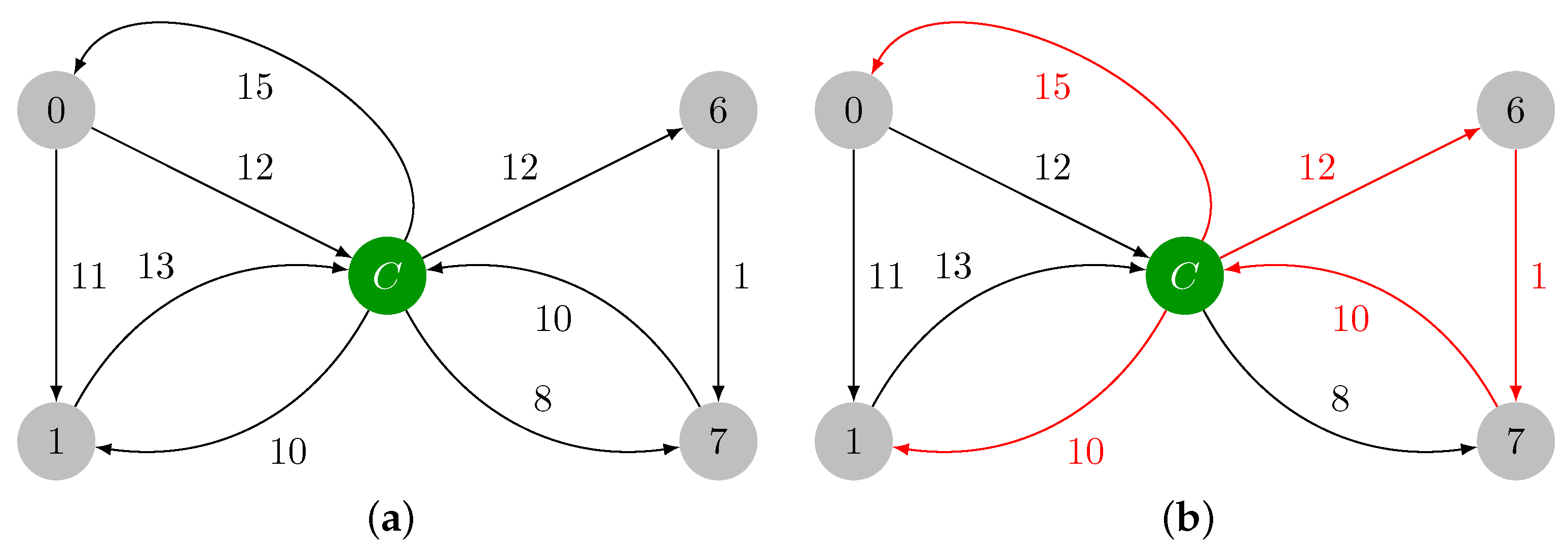
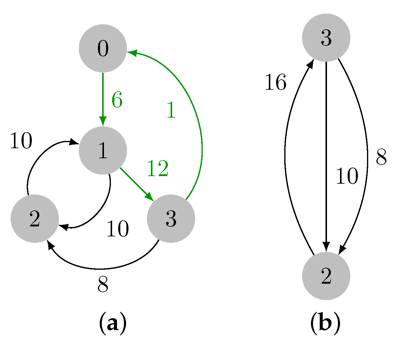
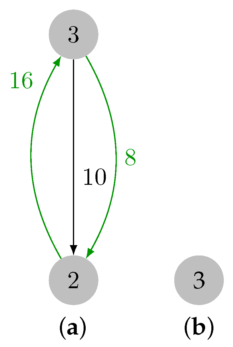
2.1.1. Contraction Phase

The algorithm proceeds by selecting vertices in G i , which are not yet in D i . If such a vertex exists, then it is added to D i , and the minimum weight incident edge on it is added to E i . The algorithm stops if either a cycle is formed in E i or if all the vertices of G i are in D i .
If E i holds a cycle, then we add the edges forming the cycle to Q i , and we build a new graph G i + 1 from G i , where the vertices in the cycle are contracted into a single super vertex v i + 1 . The edges ( u , v ) G i are added to G i + 1 and updated as follows:
  • Loop edge removal: If u , v Q i , then ( u , v ) G i + 1 .
  • Unmodified edge preservation: If u , v Q i , then ( u , v ) G i + 1 .
  • Edges originating from the new vertex: If u Q i v , Q i , then ( v i + 1 , v ) G i + 1 .
  • Edges incident to the new vertex: If u Q i v Q i , then ( u , v i + 1 ) G i + 1 , and w ( u , v i + 1 ) = w ( u , v ) + σ Q i w ( u , v ) .
Here, w ( u , v i + 1 ) is the weight of the edge ( u , v i + 1 ) in G i + 1 , w ( u , v ) is the weight of ( u , v ) in G i , σ Q i denotes the maximum edge weight in the cycle Q i , and w ( u , v ) is the weight of the edge in the cycle incident to vertex v. After the weights are updated, the algorithm continues the contraction phase with the next iteration i + 1 .
The contraction phase ends when there are no more vertices to be selected in G i for some iteration i.

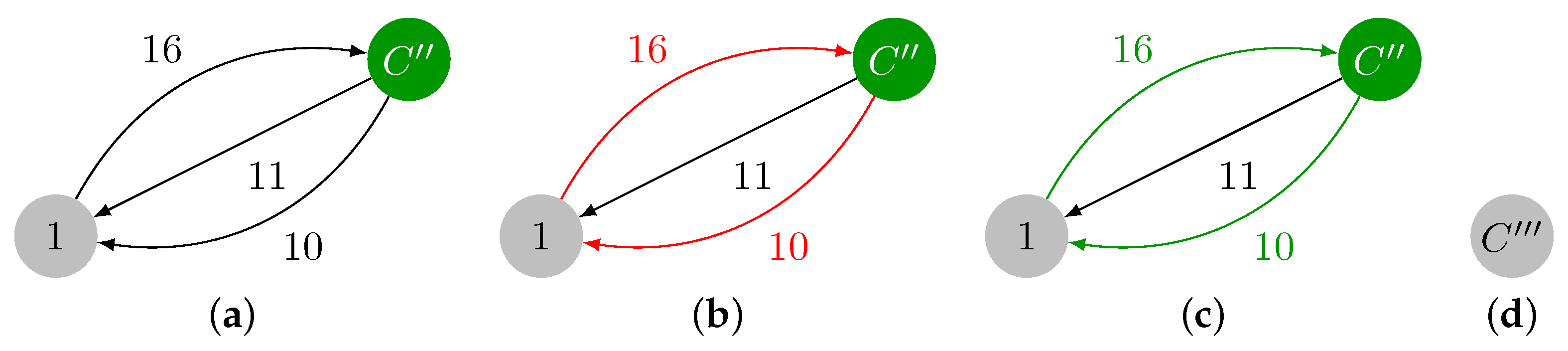
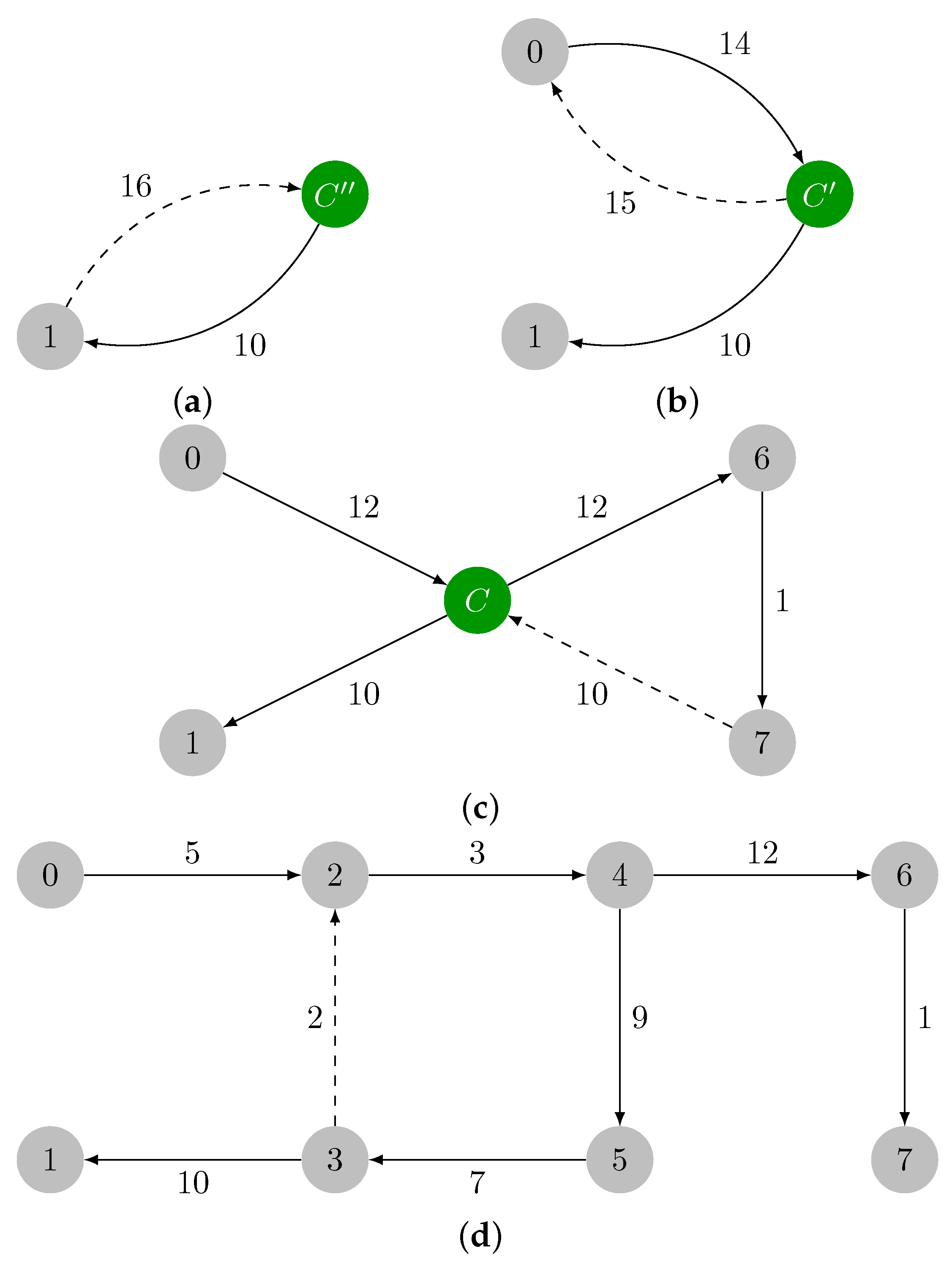
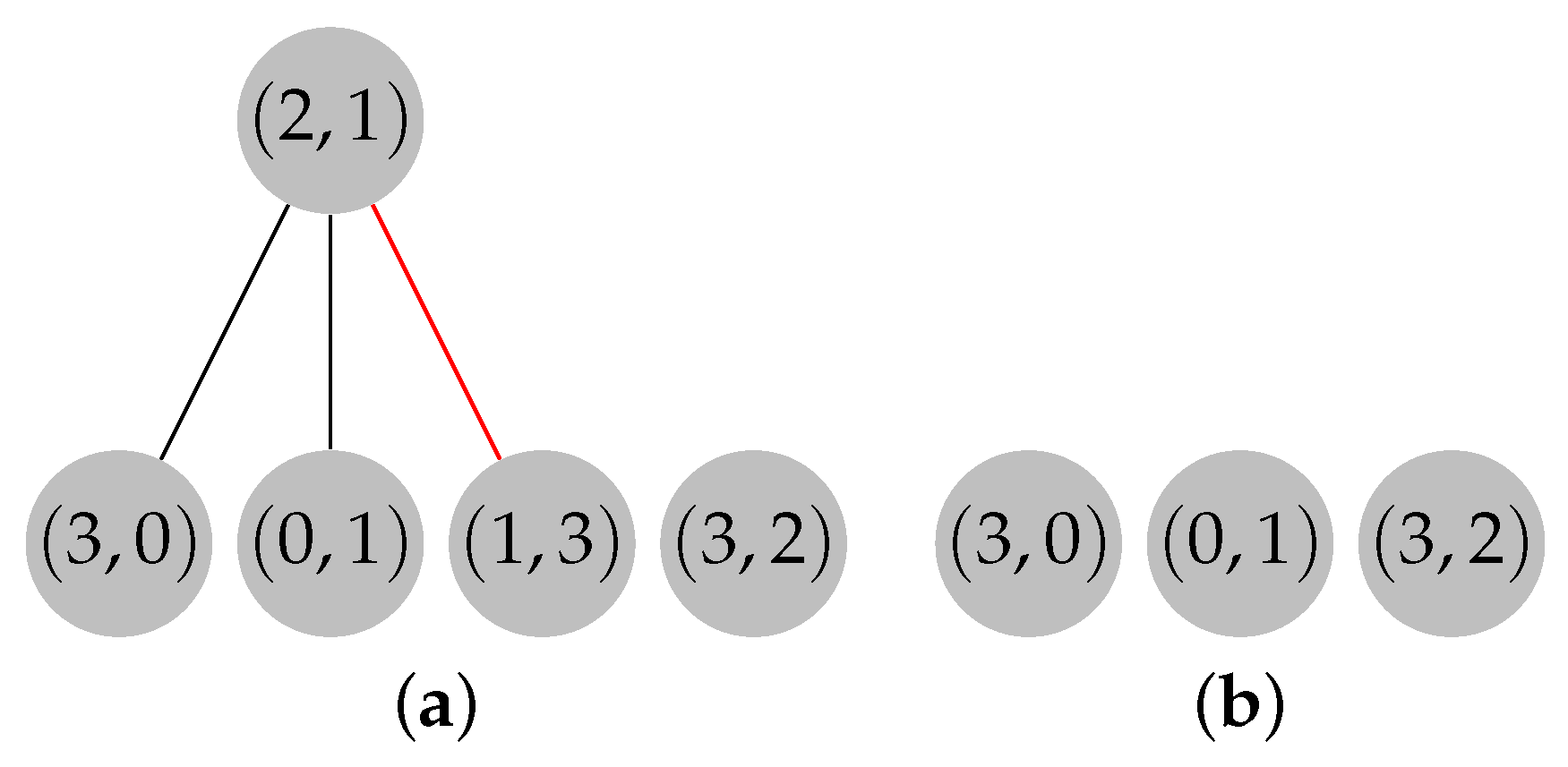
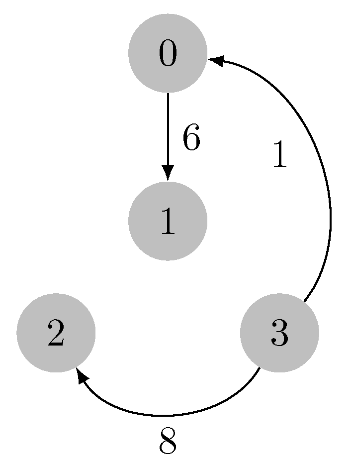
2.1.2. Expansion Phase

The final content of E i holds an arborescence for the graph G i . Let H denote a subgraph formed by the edges of E i . For every contracted cycle Q i , we add to H all the cycle edges except one. If the contracted cycle is a root of H, we discard the cycle edge with the maximum weight. If the contracted cycle is not a root of H, we discard the cycle edge that shares the same destination as an edge currently in H. The algorithm proceeds in reverse with respect to the contraction phase, thus examining the graph G i 1 and the cycle Q i 1 . This process continues until all contractions are undone, and H is the final arborescence.

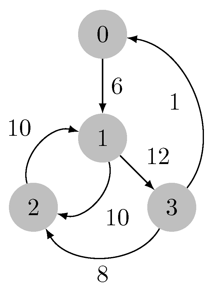
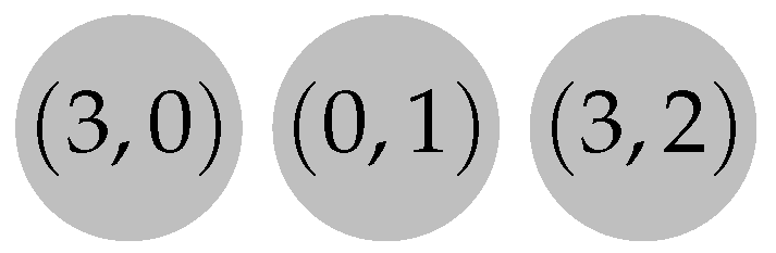
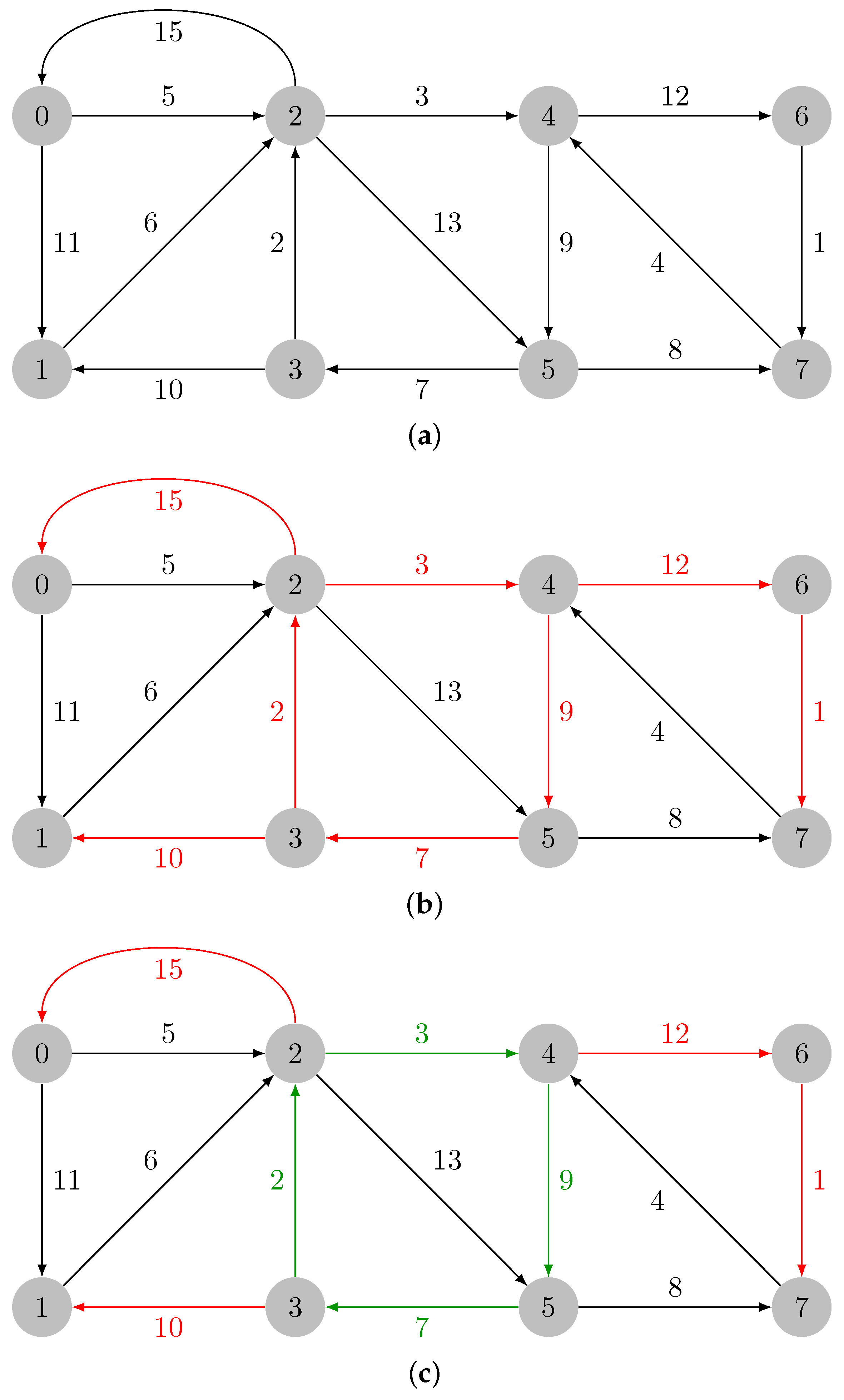
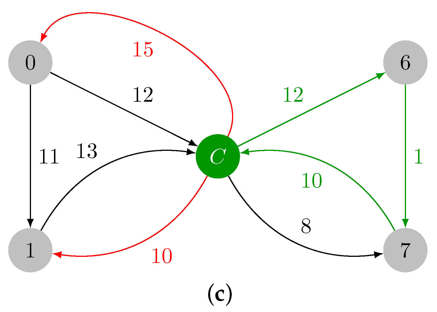
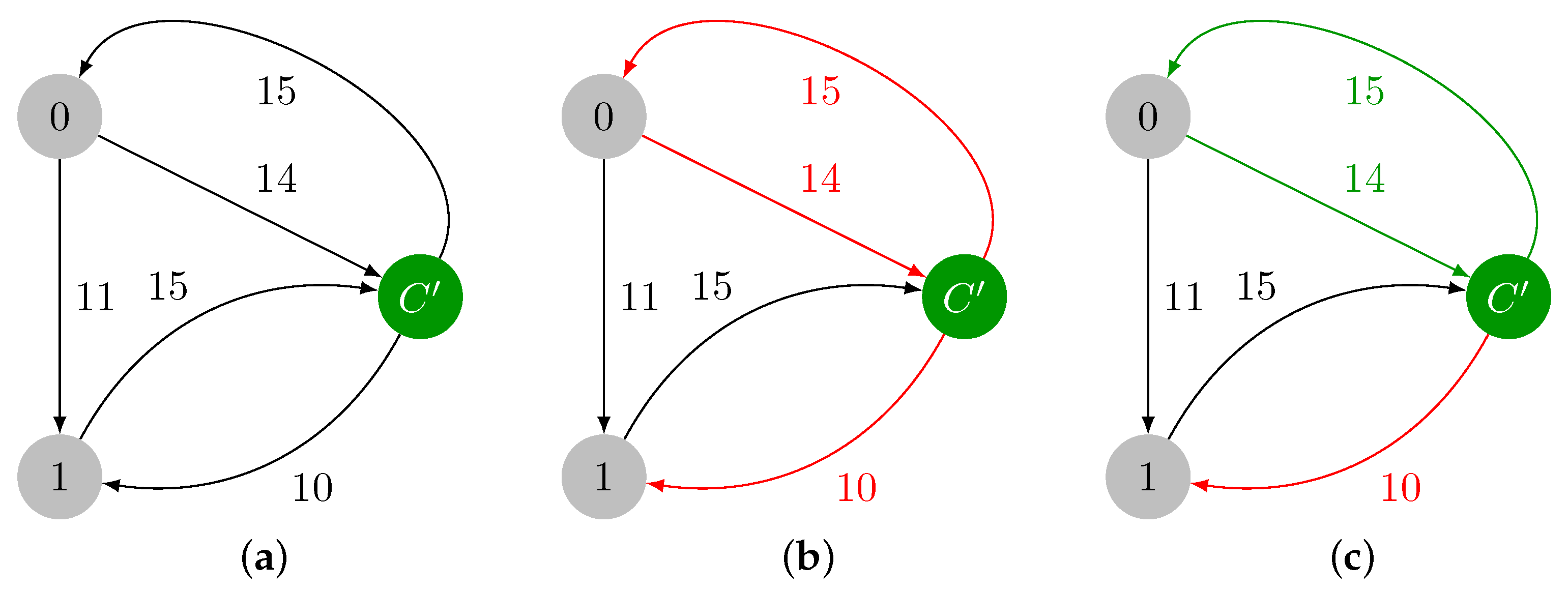
2.1.3. Illustrative Example

Let us consider the graph in Figure 1a. Let the input graph be denoted by G 0 . In Figure 1b, the minimum weight incident edges in every vertex of G 0 are colored in red; those edges are added: E 0 = { ( 2 , 0 ) , ( 3 , 1 ) , ( 3 , 2 ) , ( 2 , 4 ) , ( 5 , 3 ) , ( 4 , 6 ) , ( 6 , 7 ) } . The green edges in Figure 1c form a cycle and are added to Q 0 = { ( 3 , 2 ) , ( 2 , 4 ) , ( 4 , 5 ) , ( 5 , 3 ) } . The cycle Q 0 must then be contracted. The maximum weight edge in Q 0 is the edge ( 4 , 5 ) , and σ Q 0 = 9 .
In Figure 2a, it is shown the contracted version of G 0 , which is named G 1 , with the reduced costs already computed. In Figure 2b, the minimum weight incident edges are highlighted in red, and they are added to E 1 = { ( C , 0 ) , ( C , 1 ) , ( C , 6 ) , ( 7 , C ) , ( 6 , 7 ) } . In Figure 2c, the cycle Q 1 = { ( C , 6 ) , ( 6 , 7 ) , ( 7 , C ) } is marked in green, and it will be contracted. The maximum weight edge of Q 1 is edge ( C , 6 ) , and σ Q 1 = 12 .
The contracted version of G 1 , which is named G 2 , is presented in Figure 3a. The minimum weight incident edges in every vertex of G 2 are marked in red in Figure 3b, and they are added to E 2 = { ( 0 , C ) , ( C , 0 ) , ( C , 1 ) } . E 2 has a cycle, Q 2 = { ( 0 , C ) , ( C , 0 ) } , that is colored in green in Figure 3c. This cycle must be also contracted. The maximum weight edge of Q 2 is edge ( 0 , C ) , and σ Q 2 = 15 .
Since E 2 contains a cycle, a contraction is required, and we obtain the graph G 3 in Figure 4a. The minimum incident edges in G 3 are marked in red in Figure 4b, and they are added to E 3 = { ( 1 , C ) , ( C , 1 ) } . Note that E 3 contains another cycle: Q 3 = { ( 1 , C ) , ( C , 1 ) } . The maximum weight edge present in Q 3 is ( 1 , C ) , and σ Q 3 = 16 . A final contraction of cycle Q 3 is required, thus leading to G 4 with a single vertex, which is shown in Figure 4d. In this last iteration, we have E 4 = and Q 4 = , thereby ending the contraction phase.
The expansion phase expands the cycles formed in reverse order by kicking out one edge per cycle. The removed edges are presented as dashed edges. Let H = E 4 , and let the decrement be i. Vertex C is a root of H, since there is no edge directed towards C . In this case, every edge of Q 3 is added to H except the maximum weight edge of the cycle, as shown in Figure 5a. In iteration i = 2 , note that H = { ( C , 1 ) } , and vertex C is a root; therefore, every edge from Q 2 must be added to H except the maximum weight edge ( C , 0 ) . In the next iteration, i = 1 , vertex C is not a root of H, since edge ( 0 , C ) H . In this case, we add every edge from Q 1 except the ones that share the destination with the edges in H, as illustrated in Figure 5c. Regarding the final expansion, H = { ( 0 , C ) , ( C , 1 ) , ( C , 6 ) , ( 6 , 1 ) } implies that C is not a root. Every edge in Q 0 = { ( 3 , 2 ) , ( 2 , 4 ) , ( 4 , 5 ) , ( 5 , 3 ) } except edge ( 3 , 2 ) is added to H. The optimal arborescence of G 0 is shown in Figure 5d.

2.2. Tarjan Algorithm

The algorithm proposed by Tarjan [11] is built on the Edmonds’ algorithm, but it relies on advanced data structures to become more efficient, particularly in the contraction phase. The algorithm builds in this phase a subgraph H = ( V , E ) of G = ( V , E ) such that H contains the selected edges. The optimum arborescence could then be extracted from H through a depth-first search, thereby taking into account Lemma 2 in the Tarjan paper [11]. This lemma states that there is always a simple path in H from any vertex u in a root that is a strongly connected component S to any vertex v in the weakly connected component containing S. Camerini et al. [12], however, provided a counterexample for this construction, and they proposed a correction that relies on an auxiliary forest F, which we discuss below.
The algorithm by Tarjan keeps track of weakly and strongly connected components in G, as well as nonexamined edges entering each strongly connected component. The bookkeeping mechanism used the union–find data structure [23] to maintain disjoint sets. Let SFIND, SUNION, and SMAKE-SET denote operations on strongly connected components, and let WMAKE-SET, WFIND, and WUNION denote operations on weakly connected components. Find operations find the component where a given vertex lies in; union operations merge two components together, and make-set operations initialize the singleton components for each vertex. Nonexamined edges are kept through a collection of priority queues, which are implemented as mergeable heaps. Let MELD, EXTRACT-MIN, and INIT denote the operations on heaps, where the meld operation makes it possible to merge two heaps, the extract-min makes it possible to obtain and remove the minimum weight element, and the initialization operation makes it possible to initialize a heap from a list of elements. We also consider the SADD-WEIGHT operation, which adds a constant weight to all the edge incidents on a given strongly connected component in constant time. Note that edge incidents on a given strongly connected component are maintained in a priority queue, where they are compared taking into account its weight and the constant weight added to that strongly connected component.
The correction proposed by Camarini et al. requires us then to maintain a forest F and a set rset that holds the roots of the optimal arborescence, i.e., it holds the vertices without incident edges. Each node of forest F has an associated edge of G, a parent node, and a list of children.

2.2.1. Initialization

The data structures are initialized as follows. queues is an array of heaps, which is initialized with an heap for each vertex v containing incident edges on v. roots is the list of vertices to be processed, which is initialized as V. The forest F is initialized as empty, as well as the set r s e t . Four auxiliary arrays are also needed to build F and the optimal arborescence, namely, inEdgeNode —that for each vertex v stores a node of F associated with the minimum weight edge incident in v, π —that stores the leaf nodes of F, cycleEdgeNode —that stores for each representative cycle vertex v the list of cycle edge nodes in F, and max —that stores for each strongly connected component the target of the maximum weight edge. These data structures are initialized as detailed in Algorithm 1.
Algorithm 1 Initialization of Tarjan algorithm.
  • r o o t s                      ▹ Set of vertices to process.
  • for each v V  do
  •     queues [ v ] INIT ( v , L [ v ] )     ▹ L [ v ] refers to the list of edges incident in v.
  •     SMAKE SET ( v ) , WMAKE SET ( v )
  •     roots roots { v }
  •     max [ v ] v
  •     inEdgeNode [ v ] null
  •     π [ v ] null
  •     cycleEdgeNode [ v ]
  • end for
  • F
  • rset

2.2.2. Contraction Phase

The contraction phase proceeds while roots as follows; the while loop body is detailed in Algorithms 2–4. It pops a vertex r from roots , and it verifies if there are incident edges in r such that they do not belong to a contracted strongly connected component. If there are such edges, then it extracts the one with minimum weight; otherwise, it stops and it continues with another vertex in roots . See Algorithm 2 for the detailed pseudocode.
Algorithm 2 Main loop body of the contraction phase.
  • r POP ( r o o t s )
  • if  queues [ r ] then
  •         ( u , r ) EXTRACT MIN ( queues [ r ] )
  •        while  queues [ r ] and SFIND ( u ) = SFIND ( r )  do
  •              ( u , r ) EXTRACT MIN ( queues [ r ] )
  •        end while
  •        if  SFIND ( u ) = SFIND ( r )  then
  •              rset rset { r }
  •              continue
  •        end if
  • else
  •         rset rset { r }
  •         continue
  • end if
Once an incident edge on r is found that does not lie within a strongly connected component, i.e., that is incident on a contracted strongly connected component, we must update forest F. Hence, we create a new node minNodeF in forest F that is associated with edge ( u , r ) . If r is not part of a strongly connected component, i.e., r is not part of a cycle, then minNodeF becomes a leaf of F. Otherwise, F must be updated by making minNodeF a parent of the trees of F that are part of the strongly connected component. Algorithm 3 details this updating of forest F.
Algorithm 3 Continuation of the main loop body of the contraction phase.
  • Create the node minNodeF in forest F associated with the edge ( u , r )
  • if  cycleEdgeNode [ r ] =  then
  •        π [ r ] minNodeF
  • else
  •       for each n cycleEdgeNode [ r ]  do
  •              PARENT ( n ) minNodeF
  •              CHILDREN ( minNodeF ) CHILDREN ( minNodeF ) { n }
  •       end for
  • end if
The next step is to verify if ( u , r ) forms a cycle with the minimum weight edges formerly selected. It is enough to check if ( u , r ) connects the vertices in the same weakly connected components. Note that ( u , r ) is incident on a root and, if u lies in the same weakly connected component as r, then adding ( u , r ) necessarily forms a cycle. Assuming that adding ( u , r ) does not form a cycle, we perform the union of the sets representing the two weakly connected components to which u and r belong, i.e., WUNION ( u , r ) . We also update the inEdgeNode [ r ] array, as r now has an incident edge selected.
If adding ( u , r ) forms a cycle, a contraction is performed. The contraction procedure starts firstly by finding the edges involved in the cycle by using a backward depth-first search. During this process, a m a p is initialized, where the edge is associated to its F node (the map key). Then the maximum weight edge in the cycle is found, the reduced costs are computed, and the weight of the edges is updated. Note that the min-heap property is always maintained when reducing the costs without running any kind of procedure to ensure it, since the constant r e d u c e d is added to every edge in a given priority queue. The arrays inEdgeNode and cycleEdgeNode are updated, and the heaps involved in the cycle are merged. See Algorithm 4 for detailed pseudocode.
Algorithm 4 Continuation of the main loop body of the contraction phase.
  • if  WFIND ( u ) WFIND ( r )   then
  •       inEdgeNode [ r ] minNodeF
  •       WUNION ( u , r )
  • else
  •       inEdgeNode [ r ] null
  •       cycle { minNodeF }
  •      Let map denote a map.
  •       map [ minNodeF ] ( u , r )
  •       u SFIND ( u )
  •      while  inEdgeNode [ u ] n u l l  do
  •             cycle cycle { inEdgeNode [ u ] }
  •             ( v , u ) EDGE ( inEdgeNode [ u ] )
  •             map [ inEdgeNode [ u ] ] ( v , u )
  •             u SFIND ( v )
  •      end while
  •      Let σ denote the weight of the maximum weight edge ( u σ , v σ ) in cycle .
  •       rep SFIND ( v σ )
  •      for each node n cycle  do
  •             cost σ w ( map [ n ] )
  •             ( u , v ) E D G E ( n )
  •             SADD WEIGHT ( v , cost )
  •             cycleEdgeNode [ SFIND ( v ) ] cycleEdgeNode [ SFIND ( v ) ] { n }
  •      end for
  •      for each node n cycle  do
  •             ( u , v ) E D G E ( n )
  •             SUNION ( u , v )
  •      end for
  •       roots roots { SFIND ( rep ) }
  •       max [ SFIND ( rep ) ] = max [ rep ]
  •      for each node n cycle  do
  •             ( u , v ) E D G E ( n )
  •            if  SFIND ( v ) rep  then
  •                  MELD ( queues [ rep ] , queues [ SFIND ( v ) ] )
  •          end if
  •      end for
  • end if

2.2.3. Expansion Phase

We obtain the optimal arborescence from the forest F, which is decomposed to break the cycles of G. Note that the nodes of F will represent the edges of H seen in Edmonds’ algorithm. The expansion phase is as follows. We first take care of the super nodes of F, which are roots of the optimal arborescence, represented by the set rset . Each vertex u in rset is the representative element of a cycle, i.e., the destination of the maximum edge of a cycle. Hence, u becomes a root of the optimal arborescence, and every edge incident to u in F must be deleted. The tree F is decomposed by deleting the node π [ u ] and all its ancestors. For the other cycles, whose corresponding super vertices are not optimal arborescence roots, the incident edge ( u , v ) , represented by a root in F, is added to H, and the other incident edges represented in F by π [ v ] and its ancestors are deleted. The procedure ends when there are no more nodes in F. The optimal arborescence is given by H. The pseudocode is detailed in Algorithm 5.
Algorithm 5 Expansion phase.
  • H                      ▹ Set of edges.
  • R { max [ v ]   |   v rset }
  • N roots of F
  • while  R   do
  •       u POP ( R )
  •       N DELETE ANCESTORS ( π [ u ] , N )
  • end while
  • while  N   do
  •       ( u , v ) EDGE ( POP ( N ) )
  •       H H ( u , v )
  •       N DELETE ANCESTORS ( π [ v ] , N )
  • end while
  • return  H
  • procedure  DELETE ANCESTORS ( nodeF , N )
  •       while  nodeF n u l l  do
  •            for each edge CHILDREN ( nodeF )  do
  •                   PARENT ( edge ) = null
  •                   N N { edge }
  •             end for
  •             remove nodeF
  •              nodeF = PARENT ( n o d e )
  •      end while
  •      return N
  • end procedure

2.2.4. Illustrative Example

Let us consider the graph G = ( V , E ) in Figure 6. At the beginning of the contraction phase, the forest F is empty. There is a priority queue associated with each vertex, and the contents are Q 0 = { ( 3 , 0 , 1 ) } , Q 1 = { ( 0 , 1 , 6 ) , ( 2 , 1 , 10 ) } , Q 2 = { ( 3 , 2 , 8 ) , ( 1 , 2 , 10 ) } , and Q 3 = { ( 1 , 3 , 12 ) } .
We have also roots = { 0 , 1 , 2 , 3 } , rset = , and max [ v ] = v for v V .
We start popping vertices, denoted by r, from the set roots and finding the minimum weighted edge incident to each r. We can safely pop zero, one, and two from roots , and the respective minimum weight incident edges ( 3 , 0 ) , ( 0 , 1 ) , and ( 3 , 2 ) , with weights one, six, and eight, respectively, without forming a cycle. These edges are added to forest F as nodes, thereby leading to the state seen in Figure 7. Since each vertex in { 0 , 1 , 2 } forms a strongly connected component with a single vertex, we have π [ 0 ] = ( 3 , 0 ) , π [ 1 ] = ( 0 , 1 ) , and π [ 2 ] = ( 3 , 2 ) .
Note that currently r o o t s = { 3 } , and the contents of each priority queue are Q 0 = , Q 1 = { ( 2 , 1 , 10 ) } , Q 2 = { ( 1 , 2 , 10 ) } , and Q 3 = { ( 1 , 3 , 12 ) } . Vertex 3 is then removed from set roots , edge ( 1 , 3 ) is added as a node to F, and π [ 3 ] = ( 1 , 3 ) . Also, a cycle { ( 3 , 0 ) , ( 0 , 1 ) , ( 1 , 3 ) } is formed, thereby implying that a contraction must be performed. Let three denote the cycle representant. After the contraction, we have max [ 3 ] = 3 , since ( 1 , 3 ) is the maximum weight edge in the cycle, and we have Q 3 = { ( 2 , 1 , 16 ) } , Q 2 = { ( 1 , 2 , 10 ) } , and r o o t s = { 3 } . Figure 8 depicts this first contraction.
Vertex 3 is yet again removed from the set r o o t s ; moreover, edge ( 2 , 1 , 16 ) is popped out from Q 3 , and added to F as a node. Since edge ( 2 , 1 , 16 ) is incident in a strongly connected component that contains cycle C = { ( 3 , 0 ) , ( 0 , 1 ) , ( 1 , 3 ) } , the edges directed from ( 2 , 1 ) to every edge in C are created in F, and parent pointers are initialized in the reverse direction, as shown in Figure 9.
Recall that edge ( 3 , 2 ) was previously selected, and the addition of edge ( 2 , 1 ) forms cycle C = { ( 2 , 1 ) , ( 3 , 2 ) } . After processing C , let three be the cycle representative, and, hence, r o o t s = { 3 } , Q 3 = , and max [ 3 ] = 3 , since ( 2 , 1 ) is the maximum weight edge in the cycle, and SFIND ( 1 ) = 3 . Finally, three is removed from set roots , but Q 3 is empty, thereby ending the contraction phase. The final contracted graph is presented in Figure 10.
The expansion phase can proceed now. Let N = { ( 2 , 1 ) , ( 3 , 2 ) } , R = { 3 } , and H = . Recall that π [ 0 ] = ( 3 , 0 ) , π [ 1 ] = ( 0 , 1 ) , π [ 2 ] = ( 3 , 2 ) , and π [ 3 ] = ( 1 , 3 ) . The expansion begins by evaluating the elements from set R, which contain only vertex 3. Since π [ 3 ] = ( 1 , 3 ) , and the path P 3 is constructed by following the child-to-parent direction until a root node is found, P 3 = { ( 1 , 3 ) , ( 2 , 1 ) } . Then, P 3 is removed from F, and the content of set N is updated to be N = { ( 3 , 2 ) , ( 3 , 0 ) , ( 0 , 1 ) } , as shown in Figure 11.
Since R = , the expansion phase proceeds with an evaluation of the nodes in set N. Set N is processed similarly to set R with two minor changes: the elements of N, when removed, are added to H; since N contains the edges ( u , v ) as nodes, then the path P v is traced from the leaf node stored in π [ v ] . This process terminates when N = , and H holds the optimal arborescence. The final arborescence H = { ( 3 , 2 ) , ( 3 , 0 ) , ( 0 , 1 ) } for our example is depicted in Figure 12.

3. Optimal Dynamic Arborescences
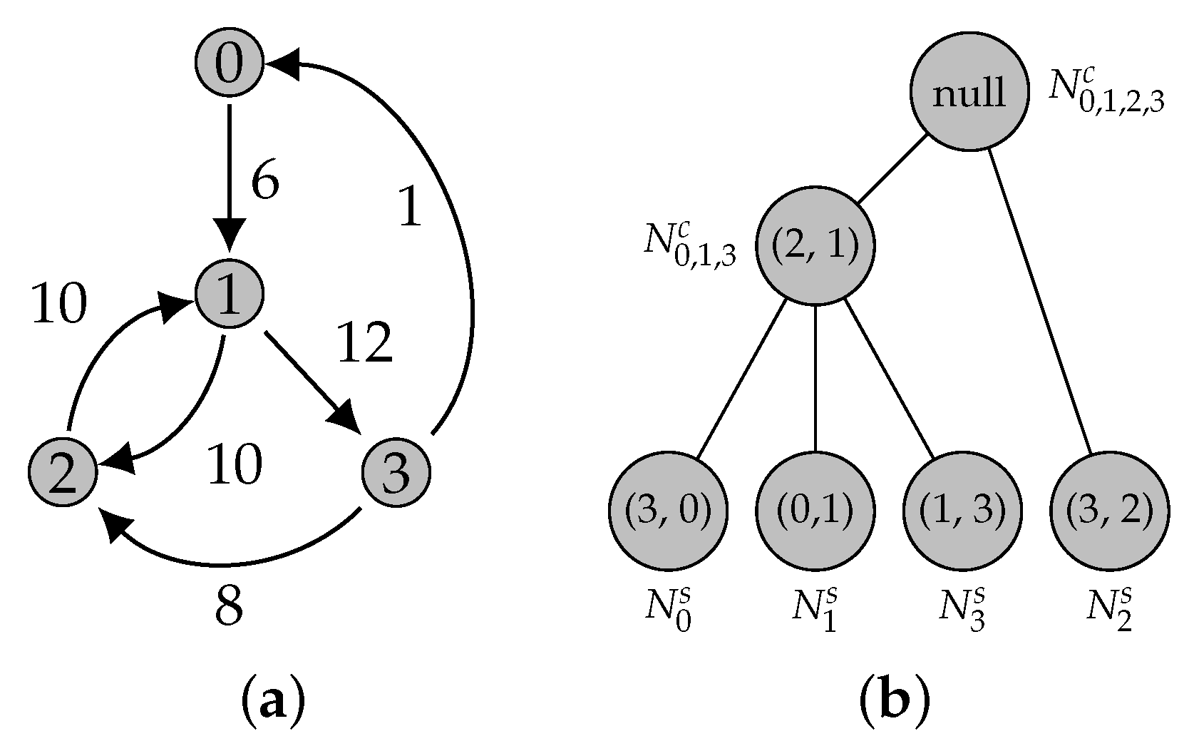
Pollatos, Telelis, and Zissimopoulos [21] proposed two variations of an intermediary tree data structure, which are built during the execution of the Edmonds’ algorithm on G and then updated when G changes. We will present the data structure by Pollatos et al. [21], named the augmented tree data structure (ATree), that encodes the set of edges H introduced in the previous section, along with all the vertices (simple and contracted) processed during the contraction phase of Edmonds’ algorithm. When G is modified, the ATree is decomposed and processed, thereby yielding a partially contracted graph G = ( V , E ) . Then, the Edmonds’ algorithm is executed for G . Note that only G and the ATree are kept in the memory.
Let us assume that the graph G = ( V , E ) is strongly connected and that w ( u , v ) > 0 for all ( u , v ) E . If G is not strongly connected, we can add a vertex v and 2 n edges such that w ( v , v ) = and w ( v , v ) = for all v V .

3.1. ATree

A simple node of the ATree, represented as N v s , encodes an edge with target v V . A complex node, represented as N i j c , encodes an edge that targets a super vertex that represents a contraction of the vertices i j V . In what follows, whenever the type of an ATree node is not known or relevant in the context, we just use N to represent it. The parent of an ATree node is the complex node, which edge targets the super vertex into which the child edge target is contracted. Since G is strongly connected, all vertices will eventually be contracted into a single super vertex, and the ATree will have a single root. A null edge is encoded in the ATree root node. See Figure 13. The ATree takes O ( n ) space, and its construction can be embedded into the Edmonds’ algorithm implementation without affecting its complexity. Let us detail how an update in G affects the ATree F, namely, the edge insertions and deletions. Edge weight updates are easily achieved by deleting the edge and adding it again with the new weight. Vertex deletions are solved by deleting all the related edges, and vertex insertions are trivially solved by considering G with the existing super vertex and the new vertex (and related edges).

3.2. Edge Deletion

Let ( u , v ) E be the edge we want to delete from G. If ( u , v ) F , we just remove it from G. If ( u , v ) F , we remove ( u , v ) from G, and we decompose the ATree: we delete the node N, which represents the edge ( u , v ) , and since we consequently break the cycles containing ( u , v ) , we also delete every ancestor node of N in F. Each child of a removed node becomes the root of its subtree. Then, we create a partially contracted graph G with the remaining nodes in the ATree, and we run the Edmonds’ algorithm for G to rebuild the full ATree F and find the new optimal arborescence.
The graph G = ( V , E ) is obtained from the decomposed ATree as follows. Note that if a complex node N i , , j c is a root of F, the super vertex representing the contraction of vertices i , , j belongs to V . Let then { N x 1 , , N x } be the roots of the ATree F, where x k is the representant of the contraction when N x k is a complex node in the ATree. Then, V = { x 1 , , x } . E is the set of the incident edges in V .

3.3. Edge Insertion

Inserting a new edge ( u , v ) is handled by reducing the problem to an edge deletion. We first add ( u , v ) in G. Then, we check if ( u , v ) should replace an edge present in ATree F. Starting from the leaf N v s of the ATree F representing an edge incident to v, and then following its ancestors, we check if w ( u , v ) is smaller than the weight of the edge represented by each N (see Figure 14). We can replace an edge if the previous condition holds and if N u s is not present in its subtree, i.e. ( u , v ) should not be an edge connecting two nodes of the current cycle. We then engage a virtual deletion of the candidate node (the edge is not deleted, but the ATree is decomposed); we build the graph G = ( V , E { ( u , v ) } ) from the decomposed ATree, and we execute the Edmonds’ algorithm for G to rebuild the full ATree F.

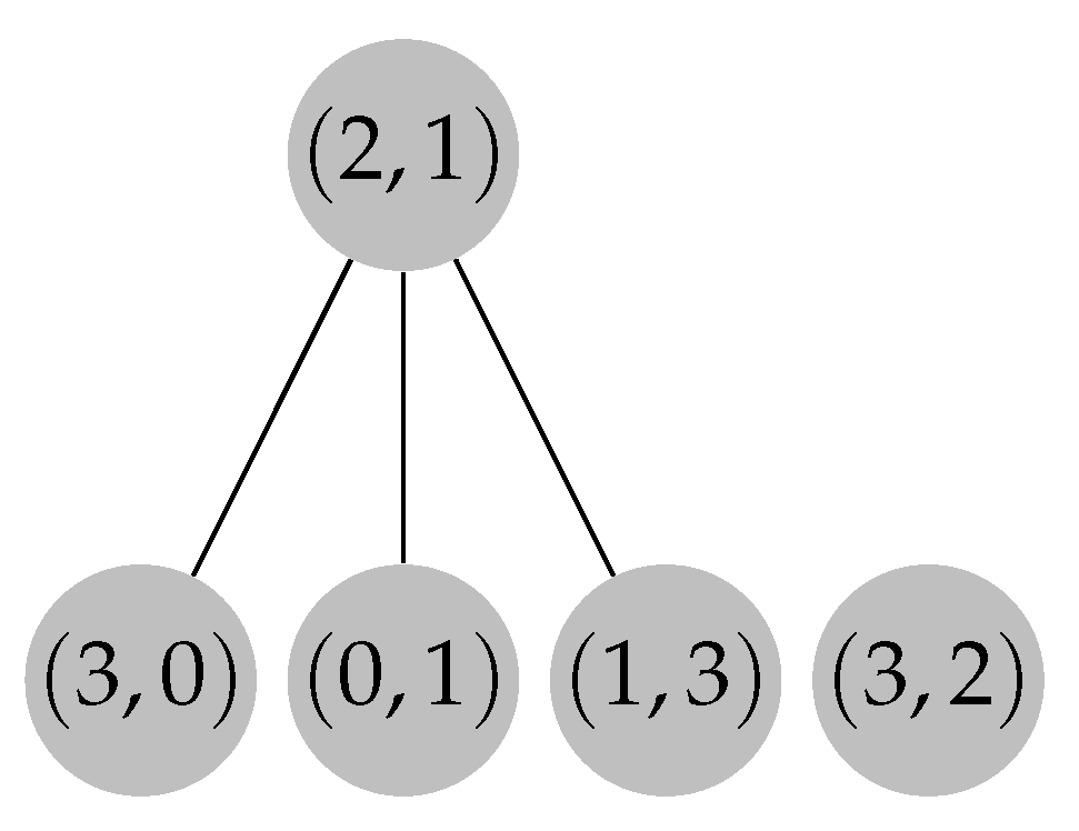
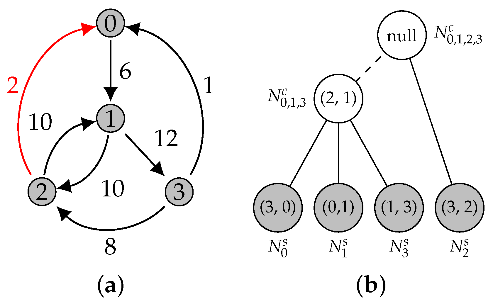
3.4. ATree Data Structure

ATree is an extension of the forest F data structure presented in Section 2.2. The nodes of the ATree maintain the following records: the edge of G, the node N, represents EDGE ( N ) ; the cost of the edge at the time it was selected is represented by w N ; its parent is represented by PARENT ( N ) ; the list of its children is represented by CHILDREN ( N ) ; its kind (simple or contracted) is measured; the list of contracted edges during the creation of the super node is documented; the edge of maximum weight in the cycle e max is measured; and its weight  w max is measured.
In an edge deletion, the edge is removed from the contracted edges list into which it belongs. In the process of decomposing and reconstructing the ATree, the set of edges E corresponds to the concatenation of the lists of contracted edges associated with each deleted ATree node. And, we need to update the weight of every edge ( u , v ) of E . Let N v s be the simple node whose contracted edges contain ( u , v ) . The new weight w ( u , v ) is w ( u , v ) = w ( u , v ) N P w N , where P is the set of ancestors of N v s , w ( u , v ) is the original weight, and w N the weight of the edge represented by N at the time it was selected. We run a BFS on each tree to find the subtracted sum r i of each simple node N i s in O ( n ) time. Then, we scan the edges e to assign the reduced cost w ( e ) = w ( e ) r i .
While adding an edge ( u , v ) , we look for a candidate node to replace in the ATree. The process starts with N v s , and it checks every ancestor until the root is inspected or if a node N verifies w ( EDGE ( N ) ) > w ( u , v ) , where w ( EDGE ( N ) ) denotes the reduced cost of the edge presented by N. If the root is reached without verifying the condition, we insert ( u , v ) in the contracted edges list of the lowest common ancestor of N v s and N u s . If the condition is met, we find a candidate node N where ( u , v ) could be added, but we must determine if ( u , v ) is safe to be added. We check if N u s is already present with a BFS in the subtree of root N. If we find N u s , and we insert ( u , v ) in the contracted edges list of the lowest common ancestor of N v s and N u s . Otherwise, we engage a virtual deletion of EDGE ( N ) (the edge is not deleted, but the ATree is decomposed); then, we build the graph G = ( V , E { ( u , v ) } ) and execute the Edmonds’ algorithm for G as mentioned before. The pseudocode for finding a candidate is detailed in Algorithm 6, where ( u , v ) is the edge to be inserted.
Algorithm 6 Finding a candidate node in the ATree; ( u , v ) is the edge to be inserted.
  • nodeF = N v s
  • if  w ( EDGE ( nodeF ) ) > w ( u , v )   then
  •        return  nodeF
  • end if
  • S                            ▹Let S be a set.
  • while  nodeF null   do
  •        S = S { nodeF } )
  •        nodeF = PARENT ( nodeF )
  • end while
  • Let L be a LIFO containing the nodes in cycle creation order.
  • compare = false
  • candidate = null
  • while  L   do
  •        nodeF = POP ( L )
  •       if  nodeF is root then
  •           return  null
  •       end if
  •       if  nodeF S  then
  •            compare = true
  •       end if
  •        candidate = FIND CANDIDATE ( nodeF , ( u , v ) , compare )
  •        compare = false
  •       if  candidate null  then
  •           break
  •       end if
  • end while
  • return  candidate
  • procedure  FIND CANDIDATE ( nodeF , e i n , compare )
  •       Let w max be the maximum weight edge in CHILDREN ( nodeF ) .
  •       for each child CHILDREN ( nodeF )  do
  •            ( u , v ) = EDGE ( c h i l d )
  •            cost = w max ( w ( u . v ) + SFIND WEIGHT ( v ) )
  •            SADD WEIGHT ( v , cost )
  •       end for
  •        ( u , v ) = EDGE ( nodeF )
  •        w ( u , v ) = w ( u , v ) + SFIND WEIGHT ( v )
  •        w ( u , v ) = w ( u , v ) + SFIND WEIGHT ( v )
  •       if  compare and w ( u , v ) < w ( u , v )  then
  •           return  nodeF
  •       end if
  •       for each edge CHILDREN ( nodeF )  do
  •            ( u , v ) = EDGE ( edge )
  •            SUNION ( u , v )
  •       end for
  •       return  null
  • end procedure

4. Implementation Details and Analysis

Let us detail and discuss our implementation, namely, used data structures and their customization, for finding an optimal arborescence and dynamically maintaining it. It follows the pseudocode described in the previous sections. As mentioned earlier, this implementation is built on the theoretical results introduced by Edmonds [9], Tarjan [11], and Camerini et al. [12] for the static algorithm, as well as on the results derived by Pollatos, Telelis, and Zissimopoulos [21] for the dynamic algorithm. The implementation incorporates all these results, namely, the contraction and expansion phases by Edmonds, the bookkeeping mechanisms proposed by Tarjan, and the forest data structure introduced by Camerini et al., which have been further extended as the ATree data structure. Recall that the bookkeeping mechanism adjusted to maintain the forest data structure relies on the following data structures: for every node v, a list L ( v ) stores each edge incident to v; disjoint sets keep track of the strongly and weakly connected components; and a collection of queues keeps track of the edges entering each vertex and a forest—or, in the dynamic case, an ATree F.

4.1. Incidence Lists

Since edges of G are processed by incidence and not by origin, G is represented as an array of edges sorted with respect to target vertices. This is beneficial, since it takes advantage of memory locality, thereby bringing improvements to the overall performance.

4.2. Disjoint Sets

Two implementations of the union–find data structure for managing disjoint sets are used, with both supporting the standard operations. One is used to represent weakly connected components, while the other is employed for strongly connected components. The latter is an augmented version. In the case of the first implementation, the following common operations are supported: WFIND ( x ) , which returns a pointer to the representative element of the unique set containing x; WUNION ( x ) , which unites the sets that contain x and y; and WMAKE SET ( x ) , which creates a new set whose only element and representative is x. For the augmented implementation, the same operations are supported, but they are named SFIND , SUNION , and SMAKE SET ; two extra operations are also supported, namely, SADD WEIGHT and SFIND WEIGHT , which are detailed below.
Our implementations of the union–find data structure rely on the conventional heuristics, namely, union by rank and path compression, thereby achieving nearly constant time per operation in practice; m operations over n elements take O ( m α ( n ) ) amortized time, where α is the inverse of the Ackermann [24]. Both implementations use two arrays of integers, namely, the rank and the parent array instead of pointer-based trees. Even though the operation’s computational complexity is, theoretically speaking, the same, using arrays instead of pointers promotes memory locality, since arrays are allocated in contiguous memory.
The purpose of having a different implementation for strongly connected components is to bring a constant time solution for the computation of the reduced costs, thereby exploiting the path compression and union by rank heuristics. While finding the minimum weight incident edges in every vertex in the contraction phase, cycles may arise. Then, the maximum weight edge in the cycle is found, the reduced costs are computed, and the weight of the incident edges is updated by summing the reduced costs. In this context, the augmented version of the union–find data structure then supports the following operations as mentioned above: SADD WEIGHT ( x , k ) , which adds a constant k to the weight of all the elements of the set containing x, and SFIND WEIGHT ( x ) , which returns the accumulated weight for the set containing x. Supporting these operations requires an additional attribute weight , which is represented internally as a third array to store the weights. The weights are initialized with 0. The SADD WEIGHT ( x , k ) operation adds value k to the root or representative element of the set containing x in constant time. The operation SFIND ( x ) has been rewritten for updating the weights whenever the underlying union–find tree structure changes due to the path compression heuristic; this change does not change the complexity of this operation. The operation SFIND WEIGHT ( x ) performs the sum of all values stored in field weight on the path from x until we meet the root of the disjoint set containing x; the cost of this operation is identical to the cost of operation of SFIND . A constant time solution is obtained then for updating the weight of all the elements in a given set, which allows us to update the weight of all the edges that are incident on a given vertex and also in constant time.

4.3. Queues

Heaps are used to implement the priority queues, which track the edges that are incident in each vertex. In this context, three types of heaps were implemented and tested, namely, binary heaps [25], binomial heaps [26], and pairing heaps [27,28]. The pairing heaps are the alternative that have simultaneously better theoretical and expected experimental results; although binary heaps are faster than all other heap implementations when the decrease key operation is not needed. Pairing heaps are often faster than d-ary heaps (like binary heaps) and almost always faster than other pointer-based heaps [29]. Our experimental results also consider this comparison (see Section 5). With respect to the theoretical results, using pairing heaps to implement priority queues and assuming that n is the size of a heap, the common heap operations are as follows: INIT ( L ) creates a heap with elements in list L in O ( n ) time; INSERT ( h , e ) inserts an element e in the heap h in Θ ( 1 ) time; GET MIN ( h ) obtains the element with minimum weight in Θ ( 1 ) time; EXTRACT MIN ( h ) returns and removes from the heap h the element with the minimum weight in O ( log n ) amortized time; DECREASE KEY ( h , e ) decreases the weight of element e in o ( log n ) amortized time; and MELD ( h 1 , h 2 ) merges two heaps h 1 and h 2 in Θ ( 1 ) time.
Our implementation does not rely on the DECREASE KEY operation, but it relies heavily on the MELD and EXTRACT MIN operations. In this context, it is important to note that the MELD operation takes O ( n ) time for binary heaps and O ( log n ) time for binomial heaps. The EXTRACT MIN ( h ) runs in O ( log n ) time for both binary and binomial heaps. On the other hand, both pairing and binomial heaps are pointer-based data structures, while binary heaps are array-based. Hence, it is not clear a priori which heap implementation would be better in practice and, hence, it is a topic of analysis in our experimental evaluation, as mentioned.

4.4. Forest

Several data structures were introduced to manage F and the cycles in G. A set rset holds the roots of the optimal arborescence, i.e., it holds the vertices that do not have any incident edge. A table max holds the destination of the maximum edges in a strongly connected component. A table π points to the leaves of F, where π [ v ] = ( u , v ) means that the node ( u , v ) of F was created during the evaluation of vertex v. The table inEdgeNode holds for each v, the unique node of F entering the strongly connected component represented by v. Finally, the list cycleEdgeNode holds the lists of nodes in a cycle, where cycleEdgeNode [ r e p ] holds the nodes of the cycle represented by r e p .
These data structures allow us to construct and maintain the forest F within the contraction phase without burdening the overall complexity of the algorithm. They allow also to extract an optimal arborescence in linear time during the expansion phase. The detailed pseudocode has been presented in Section 2.2.
This representation is extended for implementing the ATree to take into account the data structure description and the pseudocode presented in Section 3.4.

4.5. Complexity

Let us discuss the complexity of our implementation for finding a (static) optimal arborescence in a graph G with n vertices and m edges.
In the initialization phase, we mainly have the n INIT operations for the priority queues, the n SMAKE SET operations for the augmented disjoint sets, the n WMAKE SET operations for the disjoint sets, and the O ( n ) operations for the other data structures. All these operations take constant time each; thus, the initialization takes O ( n ) time.
In the contraction phase, only the operations on priority queues and disjoint sets may not take constant time. The operations on priority queues are at most the m EXTRACT MIN operations and the n MELD operations. Since EXTRACT MIN takes O ( log n ) time, and (for pairing heaps) the MELD operation takes constant time, then it takes O ( m log n ) total time for maintaining priority queues. The operations for disjoint sets are m WFIND and SFIND operations, n WUNION and SUNION operations, and n SADD WEIGHT operations. The disjoint set operations take O ( m α ( n ) ) total time, where α is the inverse of the Ackermann function [24]. The other operations run in O ( m + n ) time. Therefore, the contraction phase takes O ( m log n ) time.
In the expansion phase, F contains no more than 2 n 2 nodes, and each node of F is visited exactly once, so the procedure takes O ( n ) time. The total time required to find an optimal arborescence is therefore dominated by the priority queue operations yielding a final time complexity of O ( m log n ) .
Let us analyze now the cost of dynamically maintaining the optimal arborescence. Let ρ be the set of affected vertices and edges, | ρ | be the number of affected vertices, and | | ρ | | be the number of affected edges. A vertex is affected if it is included in a different contraction in the new output after an edge insertion or removal. Note that | ρ | < n , thus meaning that all operations in an addition or deletion of an edge occur in O ( n ) time and that a re-execution of the Edmonds’ algorithm only processes the affected vertices. The update of an optimal arborescence, using the implementation presented in Section 2.2, can then be achieved in O ( n + | | ρ | | log | ρ | ) time per edge insertion or removal.

5. Experimental Evaluation

We implemented the original Edmonds’ algorithm as described in Section 2.1 and the Tarjan algorithm as described in Section 2.2. The implementation of the Tarjan algorithm has three variants, which differ only on the heap implementation. As discussed before, we considered binary heaps, binomial heaps, and pairing heaps in our experiments. The algorithms were implemented in Java 11, and the binaries were compiled with javac  11.0 . 20 . The experiments were performed on a computer with the following hardware: Intel(R) Xeon(R) Silver 4214 CPU at 2.20GHz and with 16 GB of RAM.
The aim of this experimental evaluation is to compare the performance of Edmonds’ original algorithm with the Tarjan algorithm to evaluate the use of different heap implementations and to investigate the practicality of the dynamic algorithm for dense and sparse graphs. For the datasets, we used randomly generated graphs, both dense and sparse, and real phylogenetic data.

5.1. Datasets

Graph datasets comprising sparse and dense graphs were generated according to well known random models. To generate sparse graphs, we considered three different models. One of them was the Erdos–Rényi (ER) model [30], with p = c log n n and c 1 , where p denotes the probability of linking a node u with a node v, and n is the number of nodes in the network. Whenever p has the previously defined value, the network has one giant component and some isolated nodes. Moreover, these graphs were generated using the fast_gnp_random_graph generator of the NetworkX library [31], with p = 0.02 .
Sparse scale-free directed graphs were also generated using the model derived by Bollobás et al. [32] (identified as scale-free in our experiments) and a variant of the duplication model derived by Chung et al. [33]. The first were generated using the scale_free_graph function of the NetworkX library, with all the parameters set with their omission value except for the number of nodes. The latter were generated using our own implementation, where given 0 p 1 , the partial duplication model builds a graph G = ( V , E ) according to partial duplication as follows: start with a single vertex at time t = 1 , and, at time t > 1 , perform a duplication step: uniformly select a random vertex u of G; add a new vertex v and edges ( u , v ) and ( v , u ) with (different) random weights; for each neighbor w of u, add edges ( v , w ) and/or ( w , v ) with probability p; and find random integer weights chosen uniformly from [ 0 , 1000 ] .
Dense graphs were generated using the complete_graph generator of the NetworkX library, which creates a complete graph, i.e., all pairs of distinct nodes have an edge connecting them. Edge weights were assigned randomly.
The running time and memory were averaged over five runs and for five different graphs of each size for all models.
We also used real phylogenetic data in the dynamic updating evaluation, namely, real dense graphs using phylogenetic datasets available on EnteroBase [34]; the respective details are shown in Table 1. The graphs were built based on the pairwise distance among genetic profiles, as usual using distance-based phylogenetic inference [7]. The experiments on these data were carried out by considering increasing volumes of data, namely, [ 10 % , 20 % , 30 % , , 100 % ] .

5.2. Edmonds’ versus Tarjan

We compared both the Edmonds’ and Tarjan algorithms for complete and sparse graphs using generated graph datasets. This comparison is presented in Figure 15. As expected, the Tarjan algorithm was faster, and the experimental running time followed the expected theoretical bound of O ( m log n ) . The memory requirements were also lower for the Tarjan algorithm, which grew linearly with the size of the graph, as expected.
Given these results, we omitted Edmonds’ algorithm from the remaining evaluation.

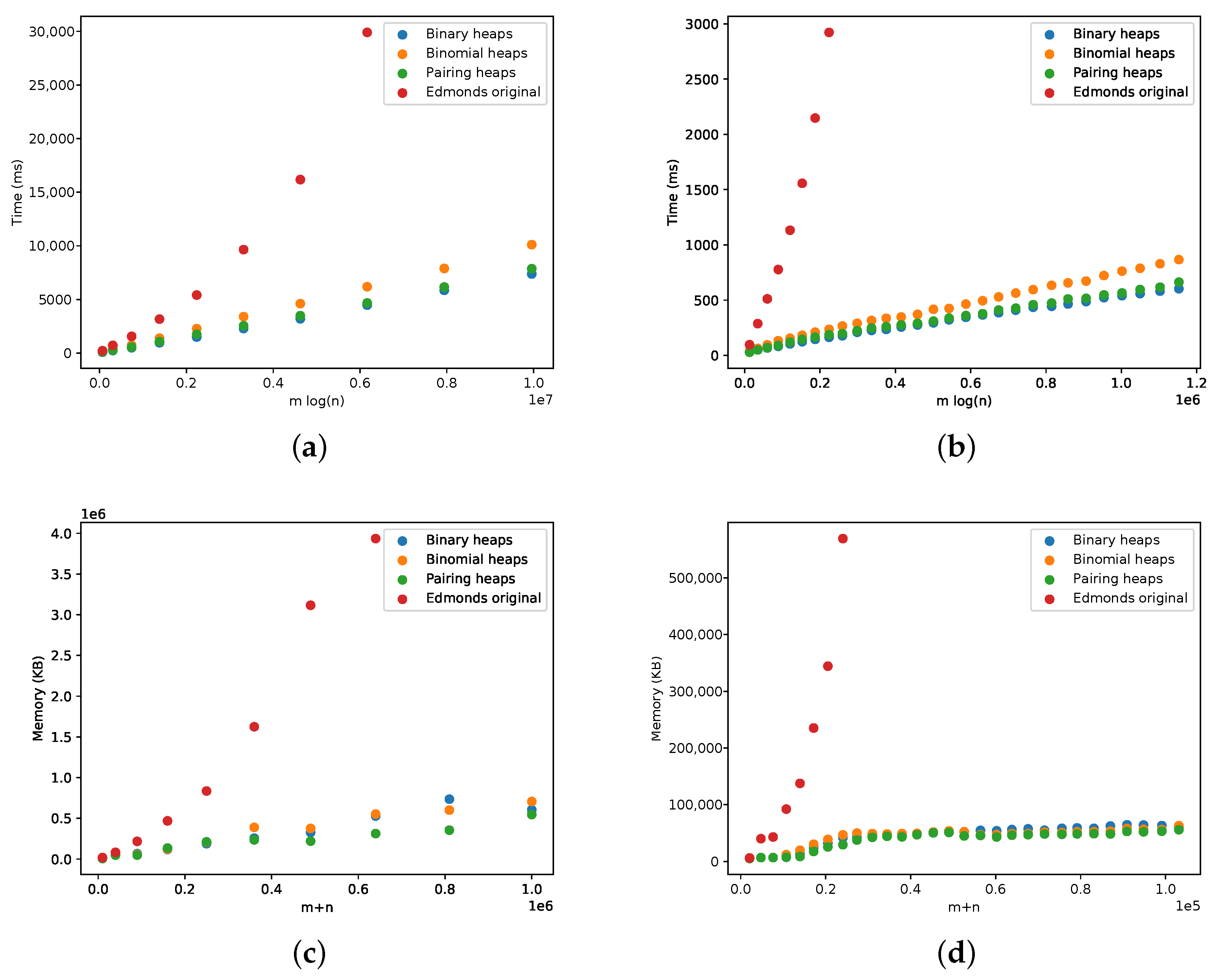
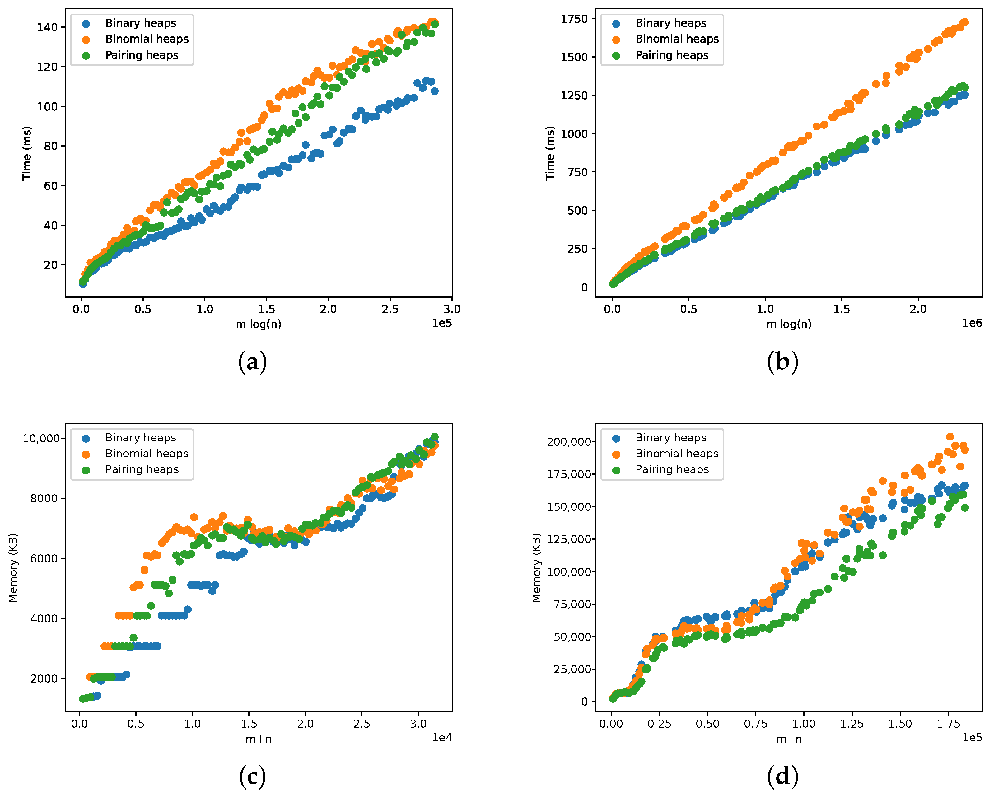
5.3. Different Heap Implementations

The results for scale-free graphs are presented in Figure 16. The running time and memory requirements are according to the expectations and to the analysis for complete and sparse graphs in the previous section. The somewhat strange behavior in the memory plots for a lower number of vertices and edges is due to Java’s garbage collector, and it can be ignored.
The focus in this section is the performance of different heap implementations when applying the Tarjan algorithm.  The improved theoretical performance of the binomial and pairing heaps was not supported by our experiments, and, in fact, they fared no better than binary heaps. The pairing heaps obtained a similar time performance to the binary heaps in the duplication models while simultaneously using less space. This is particularly interesting, since the meld operation is more efficient for pairing heaps. However, the memory locality exploited by the binary heaps played an important role here.
We note that our results are consistent with those obtained by Böther et al. [20]. Even though our implementation is in Java, while theirs is in C++, and ours is generic with respect to the total order of edges, we observed the same behavior in what concerns the running time increase versus the size of the graph, as well as with respect to binary heaps versus pointer-based heap data structures.

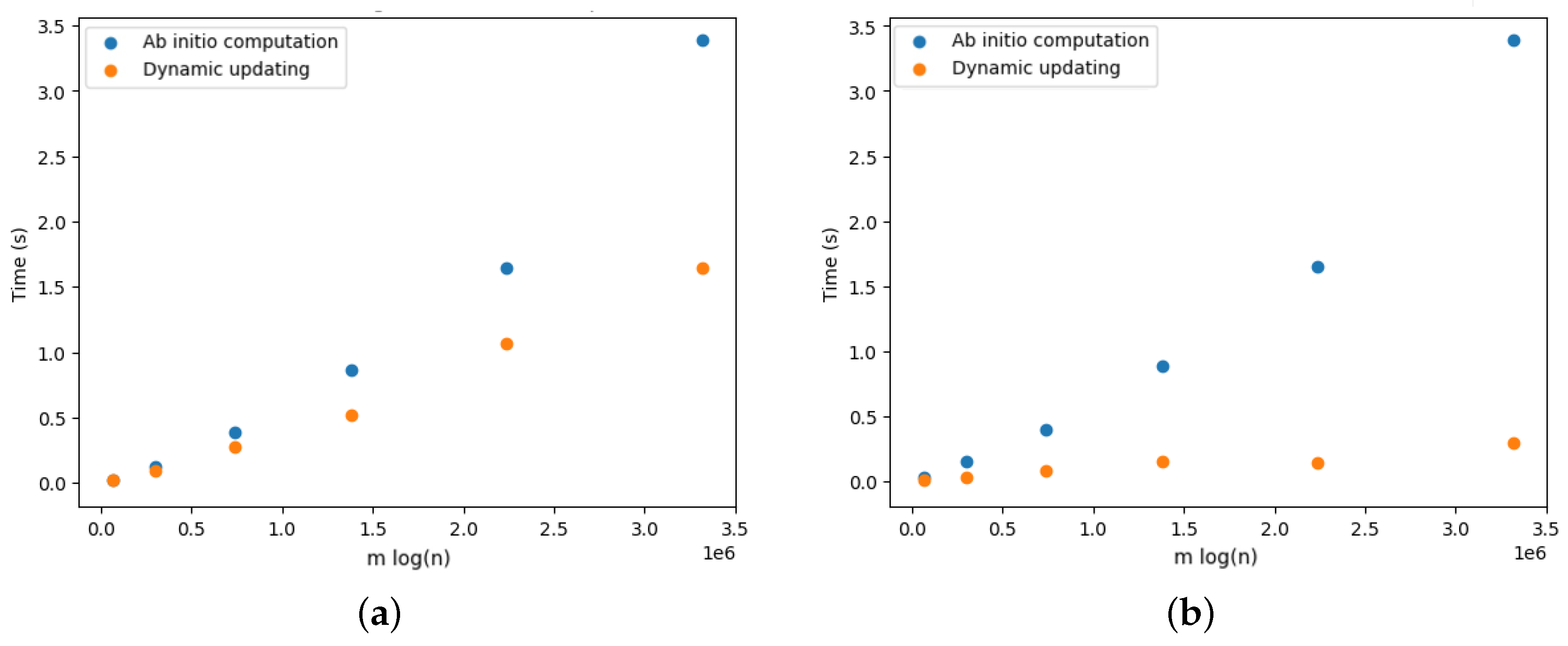
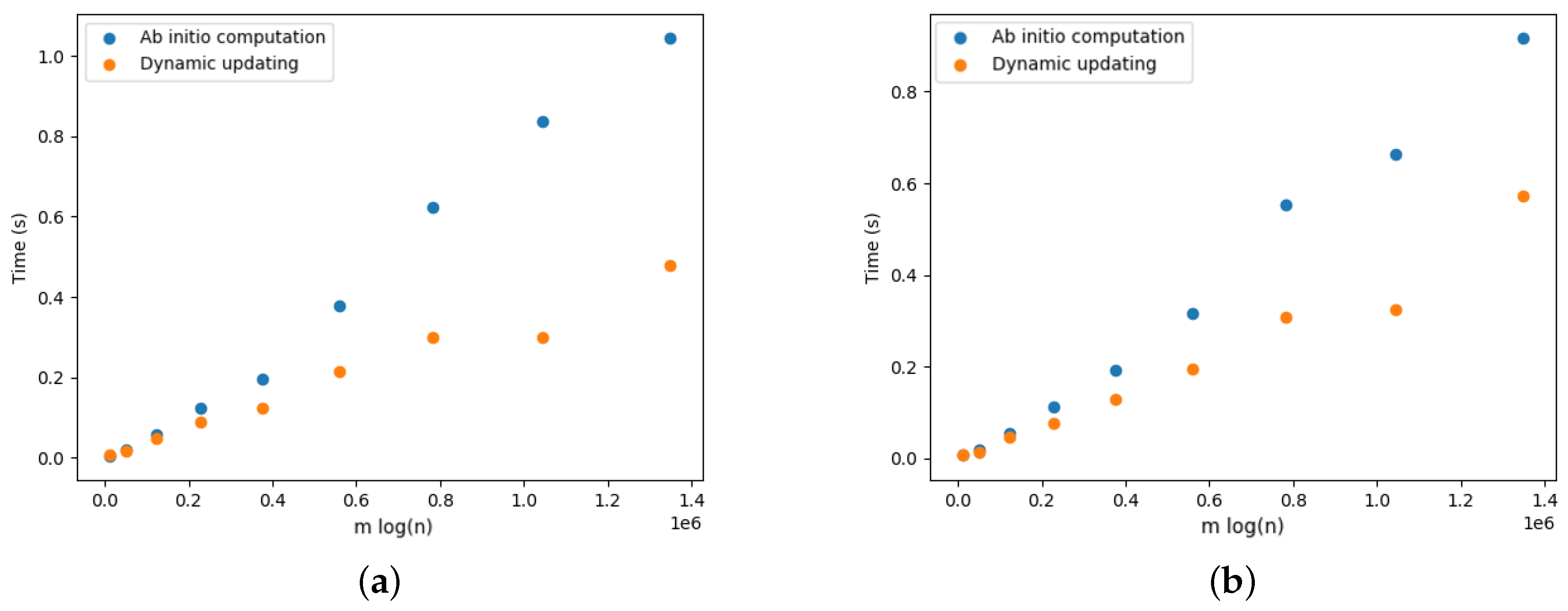
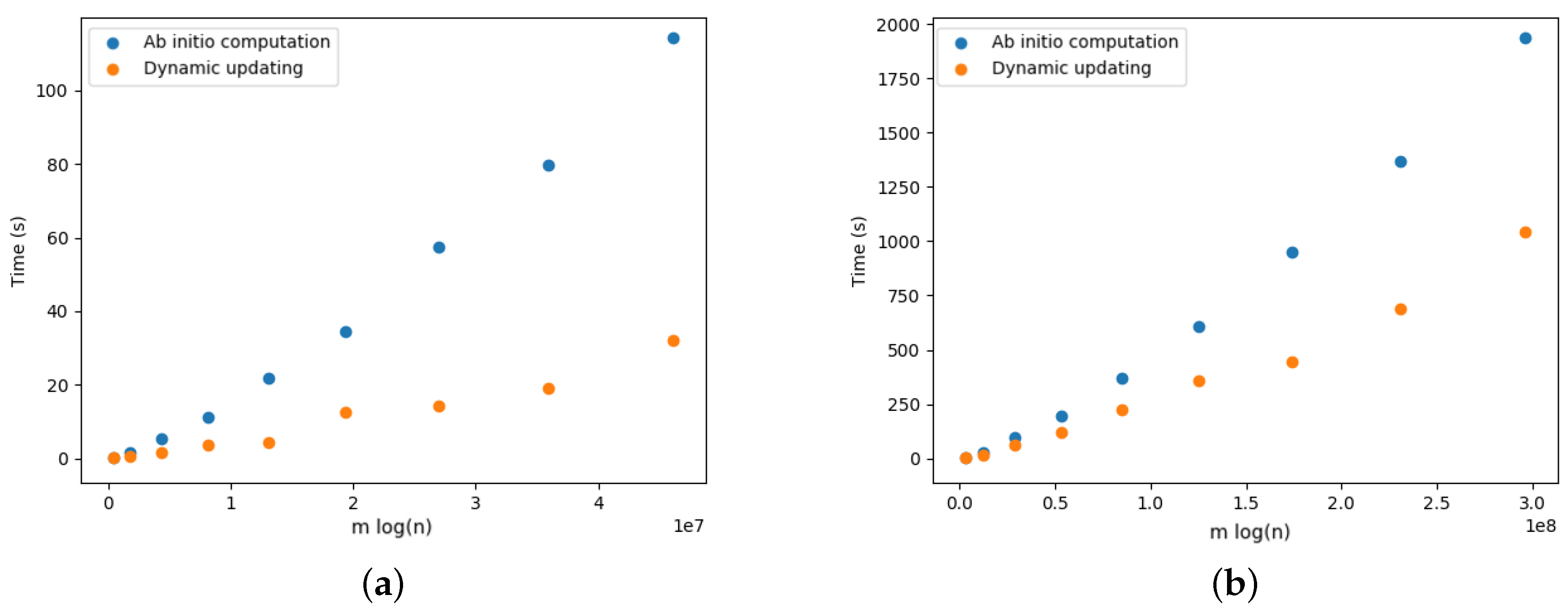
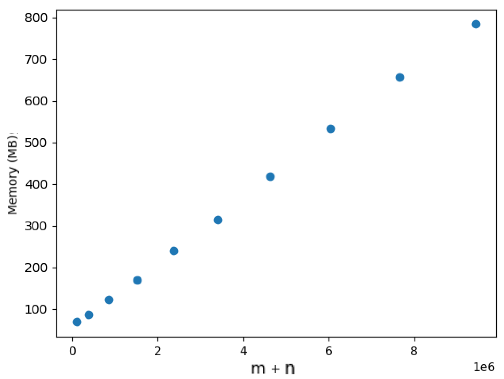
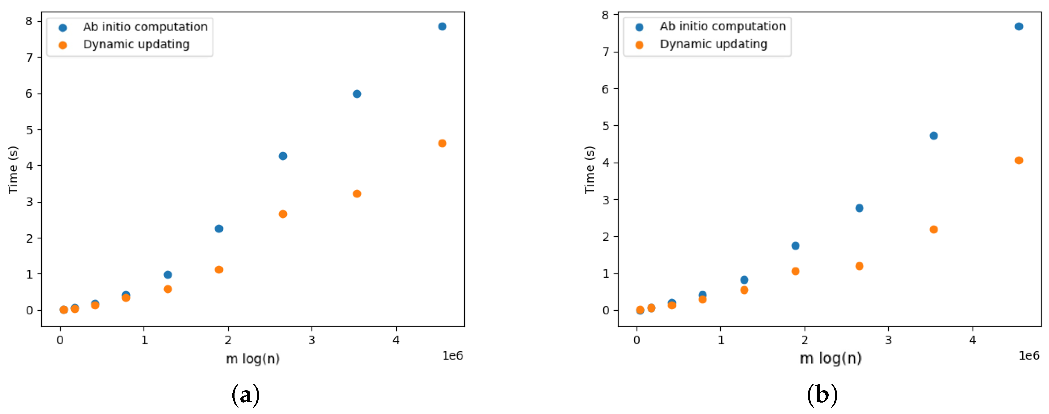
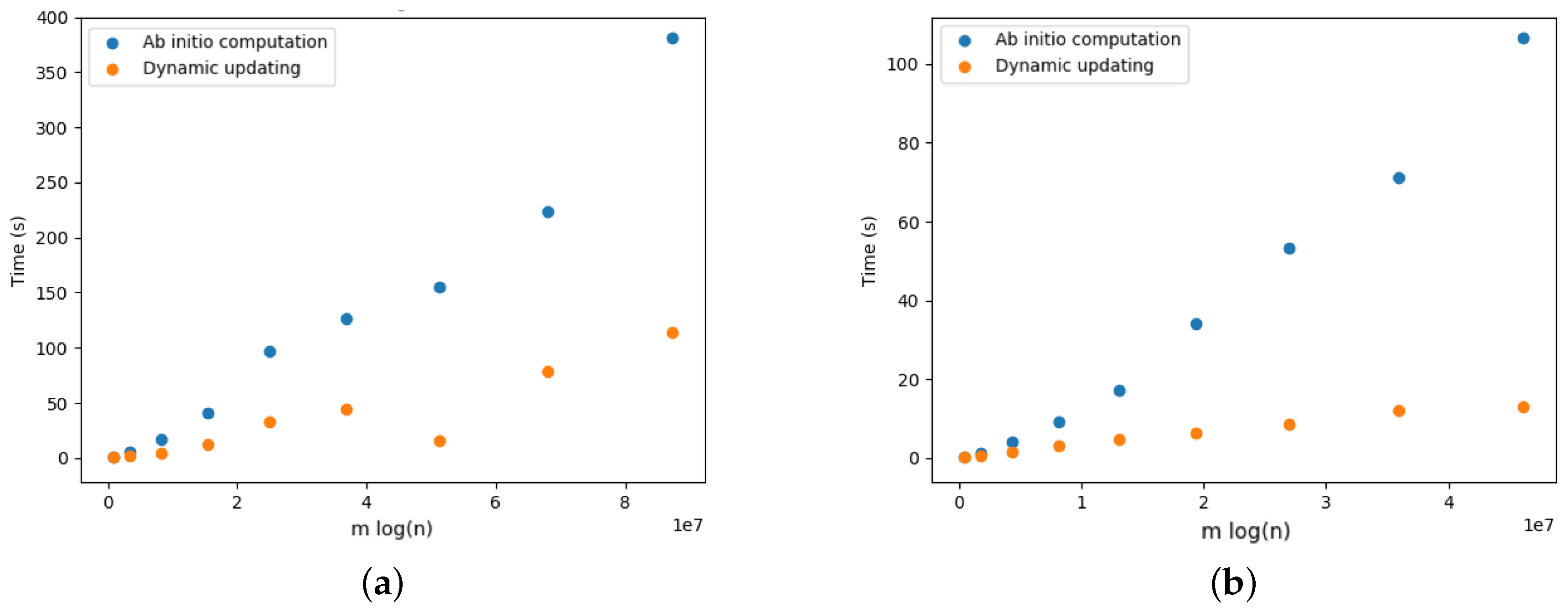
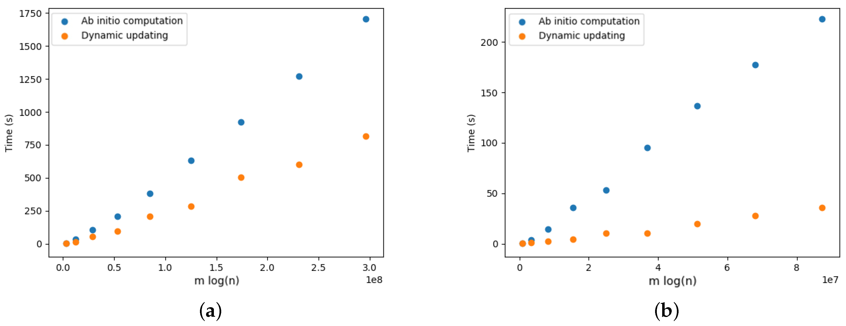
5.4. Dynamic Optimal Arborescences

Let us compare the performance of maintaining dynamic optimal arborescences versus ab initio computation on edge updates. Both implementations rely on the algorithm derived by Tarjan that is described in this paper. Our experiments consisted pf evaluating the running time and required memory for adding and deleting edges. The results were averaged over a sequence of 10 independent DELETE operations and also over a sequence of 10 independent ADD operations. The sequences of edges subject to deletion or insertion were randomly selected.
Figure 17a provides the results for the DELETE operations. We observe that updating the arborescence was twice as fast compared to its ab initio computation. Note that these results are aligned with the results presented by Pollatos, Telelis, and Zissimopoulos [21]. Figure 18a, Figure 19a, Figure 20a, Figure 21a and Figure 22a provide the results for the DELETE operation with respect to the phylogenetic data described above. As the size of the dataset grew, and the inferred graph became larger, and the dynamic updating also became more competitive, being twice as fast when compared with the ab initio computation.
The results for the ADD operations are presented in Figure 17b for complete graphs and in Figure 18b, Figure 19b, Figure 20b, Figure 21b and Figure 22b. It is clearly perceived that the ab initio computation was outmatched by the dynamic updating, in particular as the size of the graph grew. The dynamic updating was consistently at least twice as fast as the ab initio computation, thereby often surpassing that speedup factor.
We also evaluated the memory requirements for dynamic updating. We only measured the memory consumption for the DELETE operation, because the ADD operation is essentially reduced to an edge removal operation. Table 2, Table 3, Table 4, Table 5 and Table 6 show the memory usage comparison between the ab initio computation and the dynamic updating, which were averaged over 10 operations. In each table, the first column contains the % of the dataset being considered, the second column presents the memory usage for the ab initio computation, the third column presents the memory usage for the dynamic updating, and the fourth column presents the memory ratio between dynamic updating and ab initio computation. As an illustrative baseline, Figure 23 shows the memory usage for the Yersinia.wgMLST dataset as an increasing percentage of it added to the computation. Given these results, we can observe that both the ab initio computation and the dynamic updating required linear space regarding the size of the input. This is also consistent with the results for random graphs presented above. However, the dynamic updating required three times more memory on average than the ab initio computation, which is expected given that a more complex data structure needed to be managed.

6. Conclusions

We provided implementations of Edmonds’ algorithm and of the Tarjan algorithm for determining optimal arborescences on directed and weighted graphs. Our implementation of the Tarjan Algorithm incorporated the corrections by Camerini et al., and it ran in ( m log n ) time, where n is the number of vertices of the graph, and m is the number of edges. We also provided an implementation for the dynamic updating of optimal arborescences based on the ideas by Pollatos, Telelis, and Zissimopoulos that relies on the Tarjan algorithm running in O ( n + | | ρ | | log | ρ | ) per update operation, where | ρ | and | | ρ | | are, respectively, the number of affected vertices and edges that scale linearly with respect to the memory usage. We highlight the fact that our implementations are generic in the sense that a generic comparator was given as a parameter, and, hence, we were not restricted to weighted graphs; we can find the optimal arborescence on any graph equipped with a total order on the set of edges. To our knowledge, our implementation for the optimal arborescence problem for dynamic graphs is the first one to be publicly available. The code is available at https://gitlab.com/espadas/optimal-arborescences (accessed on 4 November 2023).
Experimental evaluation shows that our implementations comply with the expected theoretical bounds. Moreover, while multiple changes occurred in G, the dynamic updating was at least twice as fast as the ab initio computation, thereby requiring more memory, even if by a constant factor. Our experimental results also corroborate the results presented by Böther et al. and Pollatos et al.
We found one shortcoming regarding the dynamic optimal arborescence, namely, the high dependence between the time needed to recalculate the optimum arborescence and the affected level of the ATree. The lower the level, the larger the number of affected constituents will be. A prospect to achieve a more efficient dynamic algorithm could be relying on link–cut trees [35], which maintains a collection of node–disjoint forests of self-adjusting binary heaps (splay trees [36]) under a sequence of LINK and CUT operations. Both operation take O ( log n ) time in the worst case.
With respect to the application in the phylogenetic inference context, we highlight the fact that the proposed implementation for dynamic updates makes it possible to significantly improve the time required to update phylogenetic patterns as datasets grow in size. We note also that, due to the use of heuristics in the probable optimal tree inference, there are some algorithms that include a final step for further local optimizations [6]. Although it may not be always the case, it seems that we can often incorporate such local optimization in the total order over edges. Given that our implementations assume that such a total order is given as parameter, such optimizations can be easily incorporated. The challenge of combining these techniques to implement classes of local optimizations is also a path for future work.

Author Contributions

J.E. and A.P.F. designed and implemented the solution. J.E., L.M.S.R., T.R. and C.V. conducted the experimental evaluation. C.V., A.P.F., L.M.S.R. and T.R. wrote the manuscript. All authors have read and agreed to the published version of the manuscript.

Funding

The work reported in this article received funding from the Fundação para a Ciência e a Tecnologia (FCT), with references UIDB/50021/2020, LA/P/0078/2020, and PTDC/CCI-BIO/29676/2017 (NGPHYLO project), and from the European Union’s Horizon 2020 research and innovation program under Grant Agreement No. 951970 (OLISSIPO project). It was also supported through the Instituto Politécnico de Lisboa, with project IPL/IDI&CA2023/PhyloLearn_ISEL.

Institutional Review Board Statement

Not applicable.

Informed Consent Statement

Not applicable.

Data Availability Statement

Data are contained within the article.

Conflicts of Interest

The authors declare no conflict of interest.

References

  1. Li, Y.; Thai, M.T.; Wang, F.; Du, D.Z. On the construction of a strongly connected broadcast arborescence with bounded transmission delay. IEEE Trans. Mob. Comput. 2006, 5, 1460–1470. [Google Scholar]
  2. Fortz, B.; Gouveia, L.; Joyce-Moniz, M. Optimal design of switched Ethernet networks implementing the Multiple Spanning Tree Protocol. Discrete Appl. Math. 2018, 234, 114–130. [Google Scholar] [CrossRef]
  3. Gerhard, R. The Traveling Salesman: Computational Solutions for TSP Applications; Lecture Notes in Computer Science; Springer: Berlin/Heidelberg, Germany, 1994; Volume 840. [Google Scholar]
  4. Cong, J.; Kahng, A.B.; Leung, K.S. Efficient algorithms for the minimum shortest path Steiner arborescence problem with applications to VLSI physical design. IEEE Trans. Comput. Aided Des. Integr. Circuits Syst. 1998, 17, 24–39. [Google Scholar] [CrossRef]
  5. Coscia, M. Using arborescences to estimate hierarchicalness in directed complex networks. PLoS ONE 2018, 13, e0190825. [Google Scholar] [CrossRef]
  6. Zhou, Z.; Alikhan, N.F.; Sergeant, M.J.; Luhmann, N.; Vaz, C.; Francisco, A.P.; Carriço, J.A.; Achtman, M. GrapeTree: Visualization of core genomic relationships among 100,000 bacterial pathogens. Genome Res. 2018, 28, 1395–1404. [Google Scholar] [CrossRef]
  7. Vaz, C.; Nascimento, M.; Carriço, J.A.; Rocher, T.; Francisco, A.P. Distance-based phylogenetic inference from typing data: A unifying view. Brief. Bioinform. 2021, 22, bbaa147. [Google Scholar] [CrossRef] [PubMed]
  8. Chu, Y.J.; Liu, T. On the shortest arborescence of a directed graph. Sci. Sin. 1965, 14, 1396–1400. [Google Scholar]
  9. Edmonds, J. Optimum branchings. J. Res. Natl. Bur. Stand. B 1967, 71, 233–240. [Google Scholar] [CrossRef]
  10. Bock, F. An algorithm to construct a minimum directed spanning tree in a directed network. Dev. Oper. Res. 1971, 29, 29–44. [Google Scholar]
  11. Tarjan, R.E. Finding optimum branchings. Networks 1977, 7, 25–35. [Google Scholar] [CrossRef]
  12. Camerini, P.M.; Fratta, L.; Maffioli, F. A note on finding optimum branchings. Networks 1979, 9, 309–312. [Google Scholar] [CrossRef]
  13. Gabow, H.N.; Galil, Z.; Spencer, T.; Tarjan, R.E. Efficient algorithms for finding minimum spanning trees in undirected and directed graphs. Combinatorica 1986, 6, 109–122. [Google Scholar] [CrossRef]
  14. Fischetti, M.; Toth, P. An efficient algorithm for the min-sum arborescence problem on complete digraphs. ORSA J. Comput. 1993, 5, 426–434. [Google Scholar] [CrossRef]
  15. Aho, A.V.; Johnson, D.S.; Karp, R.M.; Kosaraju, S.R.; McGeoch, C.C.; Papadimitriou, C.H.; Pevzner, P. Emerging opportunities for theoretical computer science. ACM SIGACT News 1997, 28, 65–74. [Google Scholar] [CrossRef]
  16. Sanders, P. Algorithm engineering—An attempt at a definition. In Efficient Algorithms; Springer: Berlin, Germany, 2009; pp. 321–340. [Google Scholar]
  17. Tofigh, A.; Sjölund, E. Implementation of Edmonds’s Optimum Branching Algorithm. Available online: https://github.com/atofigh/edmonds-alg/ (accessed on 4 November 2023).
  18. Hagberg, A.; Schult, D.; Swart, P. NetworkX. Available online: https://networkx.org/documentation/stable/reference/algorithms/ (accessed on 4 November 2023).
  19. Espada, J. Large Scale Phylogenetic Inference from Noisy Data Based on Minimum Weight Spanning Arborescences. Master’s Thesis, IST, Universidade de Lisboa, Lisbon, Portugal, 2019. [Google Scholar]
  20. Böther, M.; Kißig, O.; Weyand, C. Efficiently computing directed minimum spanning trees. In Proceedings of the 2023 Symposium on Algorithm Engineering and Experiments (ALENEX), Florence, Italy, 22–23 January 2023; pp. 86–95. [Google Scholar]
  21. Pollatos, G.G.; Telelis, O.A.; Zissimopoulos, V. Updating directed minimum cost spanning trees. In Proceedings of the International Workshop on Experimental and Efficient Algorithms, Menorca, Spain, 24–27 May 2006; pp. 291–302. [Google Scholar]
  22. Barabási, A.L. Network Science; Cambridge University Press: Cambridge, UK, 2016. [Google Scholar]
  23. Galler, B.A.; Fisher, M.J. An improved equivalence algorithm. Commun. ACM 1964, 7, 301–303. [Google Scholar] [CrossRef]
  24. Tarjan, R.E.; Van Leeuwen, J. Worst-case analysis of set union algorithms. J. ACM (JACM) 1984, 31, 245–281. [Google Scholar] [CrossRef]
  25. Williams, J. Algorithm 232: Heapsort. Commun. ACM 1964, 7, 347–348. [Google Scholar]
  26. Vuillemin, J. A data structure for manipulating priority queues. Commun. ACM 1978, 21, 309–315. [Google Scholar] [CrossRef]
  27. Fredman, M.L.; Sedgewick, R.; Sleator, D.D.; Tarjan, R.E. The pairing heap: A new form of self-adjusting heap. Algorithmica 1986, 1, 111–129. [Google Scholar] [CrossRef]
  28. Pettie, S. Towards a final analysis of pairing heaps. In Proceedings of the 46th Annual IEEE Symposium on Foundations of Computer Science (FOCS’05), Pittsburgh, PA, USA, 23–25 October 2005; pp. 174–183. [Google Scholar]
  29. Larkin, D.H.; Sen, S.; Tarjan, R.E. A back-to-basics empirical study of priority queues. In Proceedings of the 2014 Sixteenth Workshop on Algorithm Engineering and Experiments (ALENEX), Portland, OR, USA, 5 January 2014; pp. 61–72. [Google Scholar]
  30. Gilbert, E.N. Random graphs. Ann. Math. Stat. 1959, 30, 1141–1144. [Google Scholar] [CrossRef]
  31. Hagberg, A.A.; Schult, D.A.; Swart, P.J. Exploring Network Structure, Dynamics, and Function using NetworkX. In Proceedings of the 7th Python in Science Conference, Pasadena, CA, USA, 19–24 August 2008; Varoquaux, G., Vaught, T., Millman, J., Eds.; pp. 11–15. [Google Scholar]
  32. Bollobás, B.; Borgs, C.; Chayes, J.T.; Riordan, O. Directed scale-free graphs. In Proceedings of the SODA, Baltimore, MD, USA, 12–14 January 2003; Volume 3, pp. 132–139. [Google Scholar]
  33. Chung, F.R.K.; Lu, L.; Dewey, T.G.; Galas, D.J. Duplication Models for Biological Networks. J. Comput. Biol. 2003, 10, 677–687. [Google Scholar] [CrossRef]
  34. Zhou, Z.; Alikhan, N.F.; Mohamed, K.; Fan, Y.; Achtman, M.; Brown, D.; Chattaway, M.; Dallman, T.; Delahay, R.; Kornschober, C.; et al. The EnteroBase user’s guide, with case studies on Salmonella transmissions, Yersinia pestis phylogeny, and Escherichia core genomic diversity. Genome Res. 2020, 30, 138–152. [Google Scholar] [CrossRef] [PubMed]
  35. Sleator, D.D.; Tarjan, R.E. A Data Structure for Dynamic Trees. J. Comput. Syst. Sci. 1983, 26, 362–391. [Google Scholar] [CrossRef]
  36. Russo, L.M. A study on splay trees. Theor. Comput. Sci. 2019, 776, 1–18. [Google Scholar] [CrossRef]
Figure 1. Identification of the cycle Q 0 in G 0 . (a) Input weighted directed graph. (b) Minimum weight incident edges in every vertex of graph G 0 , which are colored in red. (c) Cycle in G 0 colored in green.
Algorithms 16 00559 g001
Figure 2. Contraction of cycle Q 0 and identification of cycle Q 1 . (a) Contracted version of graph G 0 , which is named G 1 . (b) Minimum weight incident edges in every vertex of graph G 1 . (c) Cycle Q 1 in graph G 1 colored in green.
Algorithms 16 00559 g002aAlgorithms 16 00559 g002b
Figure 3. Contraction of cycle Q 1 and identification of cycle Q 2 . (a) Contracted version of G 1 , which is named G 2 . (b) Minimum weight incident edges in G 2 . (c) Cycle in G 2 colored in green.
Algorithms 16 00559 g003
Figure 4. Contraction of Q 2 , identification of Q 3 , and final graph G 4 after Q 3 contraction. (a) Contracted version of G 2 , which is named G 3 . (b) Minimum weight incident edges in G 3 . (c) Cycle Q 3 in G 3 colored in green. (d) G 4 .
Algorithms 16 00559 g004
Figure 5. Expansion phase and optimal arborescence. (a) Expansion subgraph H for iteration i = 3 . (b) Expansion subgraph H for iteration i = 2 . (c) Expansion subgraph H for iteration i = 1 . (d) Expansion subgraph H for iteration i = 0 .
Algorithms 16 00559 g005
Figure 6. Input weighted directed graph.
Algorithms 16 00559 g006
Figure 7. Forest F after popping 0, 1, and 2 from set roots .
Algorithms 16 00559 g007
Figure 8. First contraction of the input graph. (a) Cycle { ( 3 , 0 ) , ( 0 , 1 ) , ( 1 , 3 ) } colored in green. (b) Contraction result.
Algorithms 16 00559 g008
Figure 9. Adding directed edges from node ( 2 , 1 ) to the nodes of cycle C in forest F.
Algorithms 16 00559 g009
Figure 10. Last cycle and final contracted graph. (a) Cycle { ( 2 , 1 ) , ( 3 , 2 ) } marked in green. (b) Contraction result.
Algorithms 16 00559 g010
Figure 11. Forest F after removing P 3 . (a) Path P 3 colored in red. (b) Removal of path P 3 from forest F.
Algorithms 16 00559 g011
Figure 12. MSA of the input graph.
Algorithms 16 00559 g012
Figure 13. A graph and its ATree. The root represents the edge incident to the contraction of all graph nodes ( null ). (a) A weighted directed graph. (b) The corresponding ATree.
Algorithms 16 00559 g013
Figure 14. We add the edge ( 2 , 0 ) with weight 2 to the graph ((a): edge represented in red). The process starts with the analysis of node N 0 s , which represents edge ( 3 , 0 ) with weight 1. The vertex ( 2 , 0 ) cannot replace the N 0 s edge, as it is heavier. Then, the N 0 s parent is examined, N 0 , 1 , 3 c . The corresponding edge is heavier than ( 2 , 0 ) , and N 2 s is not present in its subtree. Then, ( 2 , 0 ) should replace this node, and N 0 , 1 , 3 c and its ancestors are virtually deleted ((b): nodes represented in white). The Edmonds’ algorithm is executed on the remaining nodes (represented in gray).
Algorithms 16 00559 g014
Figure 15. Comparison between the Edmonds’ algorithm and the Tarjan algorithm (three different heap implementation) with respect to complete and sparse graphs. (a) Running time for complete graphs. (b) Running time for sparse graphs. (c) Memory for complete graphs. (d) Memory for sparse graphs.
Algorithms 16 00559 g015
Figure 16. Comparison of three different heap implementations within the Tarjan algorithm sparse scale-free graphs. (a) Running time for scale-free graphs. (b) Running time for duplication model graphs. (c) Memory for scale-free graphs. (d) Memory for duplication model graphs.
Algorithms 16 00559 g016
Figure 17. Optimal arborescence updating versus ab initio computation for DELETE and ADD operations for complete graphs. Running time averaged over 10 random operations. (a) DELETE operations. (b) ADD operations.
Algorithms 16 00559 g017
Figure 18. Optimal arborescence updating versus ab initio computation for DELETE and ADD operations for clostridium.Griffiths dataset. Running time averaged over 10 random operations. (a) DELETE operations. (b) ADD operations.
Algorithms 16 00559 g018
Figure 19. Optimal arborescence updating versus ab initio computation for DELETE and ADD operations for Moraxella.Achtman7GeneMLST dataset. Running time averaged over 10 random operations. (a) DELETE operations. (b) ADD operations.
Algorithms 16 00559 g019
Figure 20. Optimal arborescence updating versus ab initio computation for DELETE and ADD operations for Salmonella.Achtman7GeneMLST dataset. Running time averaged over 10 random operations. (a) DELETE operations. (b) ADD operations.
Algorithms 16 00559 g020
Figure 21. Optimal arborescence updating versus ab initio computation for DELETE and ADD operations for Yersinia.cgMLSTv1 dataset. Running time averaged over 10 random operations. (a) DELETE operations. (b) ADD operations.
Algorithms 16 00559 g021
Figure 22. Optimal arborescence updating versus ab initio computation for DELETE and ADD operations for Yersinia.wgMLST dataset. Running time averaged over 10 random operations. (a) DELETE operations. (b) ADD operations.
Algorithms 16 00559 g022
Figure 23. Memory usage of Tarjan algorithm for Yersinia.wgMLST dataset.
Algorithms 16 00559 g023
Table 1. Phylogenetic datasets. The first three without missing data. The number of vertices n is the number of genetic profiles in each dataset.
Datasets n = | V | m = | E |
clostridium.Griffiths440 193 , 600
Moraxella.Achtman7GeneMLST773 597 , 529
Salmonella.Achtman7GeneMLST5464 29 , 855 , 296
Yersinia.McNally369 136 , 161
Table 2. Memory usage comparison for the dynamic updating and ab initio computation of an optimal arborescence for the clostridium.Griffiths dataset.
Dataset
%
Ab Initio
(MB)
Dynamic Updating
(MB)
Memory Ratio
106.9421.053.03
207.8724.143.07
308.9027.733.12
4010.5432.523.09
5012.5439.123.12
6014.9346.763.11
7017.9855.343.08
8021.4265.213.05
9026.2977.172.94
10031.1889.372.87
Table 3. Memory usage comparison for the dynamic updating and ab initio computation of an optimal arborescence for the Moraxella.Achtman7GeneMLST dataset.
Dataset
%
Ab Initio
(MB)
Dynamic Updating
(MB)
Memory Ratio
107.9323.973.02
209.7130.163.11
3013.1740.633.09
4017.1054.863.21
5023.8074.083.21
6030.80106.203.45
7043.92133.993.05
8049.65163.363.29
9063.66219.693.45
10079.70263.233.30
Table 4. Memory usage comparison for the dynamic updating and ab initio computation of an optimal arborescence for the Yersinia.cgMLSTv1 dataset.
Dataset
%
Ab Initio
(MB)
Dynamic Updating
(MB)
Memory Ratio
1020.9685.104.06
2038.98142.423.65
3078.79240.363.05
40131.39415.183.16
50195.35565.252.89
60261.86841.663.21
70376.261100.502.92
80465.271374.022.95
90612.671684.402.75
100724.011997.672.76
Table 5. Memory usage comparison for the dynamic updating and ab initio computation of an optimal arborescence for the Yersinia.wgMLST dataset.
Dataset
%
Ab Initio
(MB)
Dynamic Updating
(MB)
Memory Ratio
10125.32415.933.32
20156.31513.53.29
30214.65680.623.17
40295.80908.013.07
50411.261201.332.92
60534.451585.992.97
70714.392056.442.88
80898.642479.412.76
901098.493026.202.75
1001306.953640.202.79
Table 6. Memory usage comparison for the dynamic updating and ab initio computation of an optimal arborescence for the Salmonella.Achtman7GeneMLST dataset.
Dataset
%
Ab Initio
(MB)
Dynamic Updating
(MB)
Memory Ratio
1062.60210.453.36
20154.52520.833.37
30319.871041.223.26
40575.051772.005.54
50886.042667.963.01
601274.593883.463.04
701754.895242.212.99
802285.916841.032.99
902872.808574.122.99
1003435.5110,482.843.05
Disclaimer/Publisher’s Note: The statements, opinions and data contained in all publications are solely those of the individual author(s) and contributor(s) and not of MDPI and/or the editor(s). MDPI and/or the editor(s) disclaim responsibility for any injury to people or property resulting from any ideas, methods, instructions or products referred to in the content.

