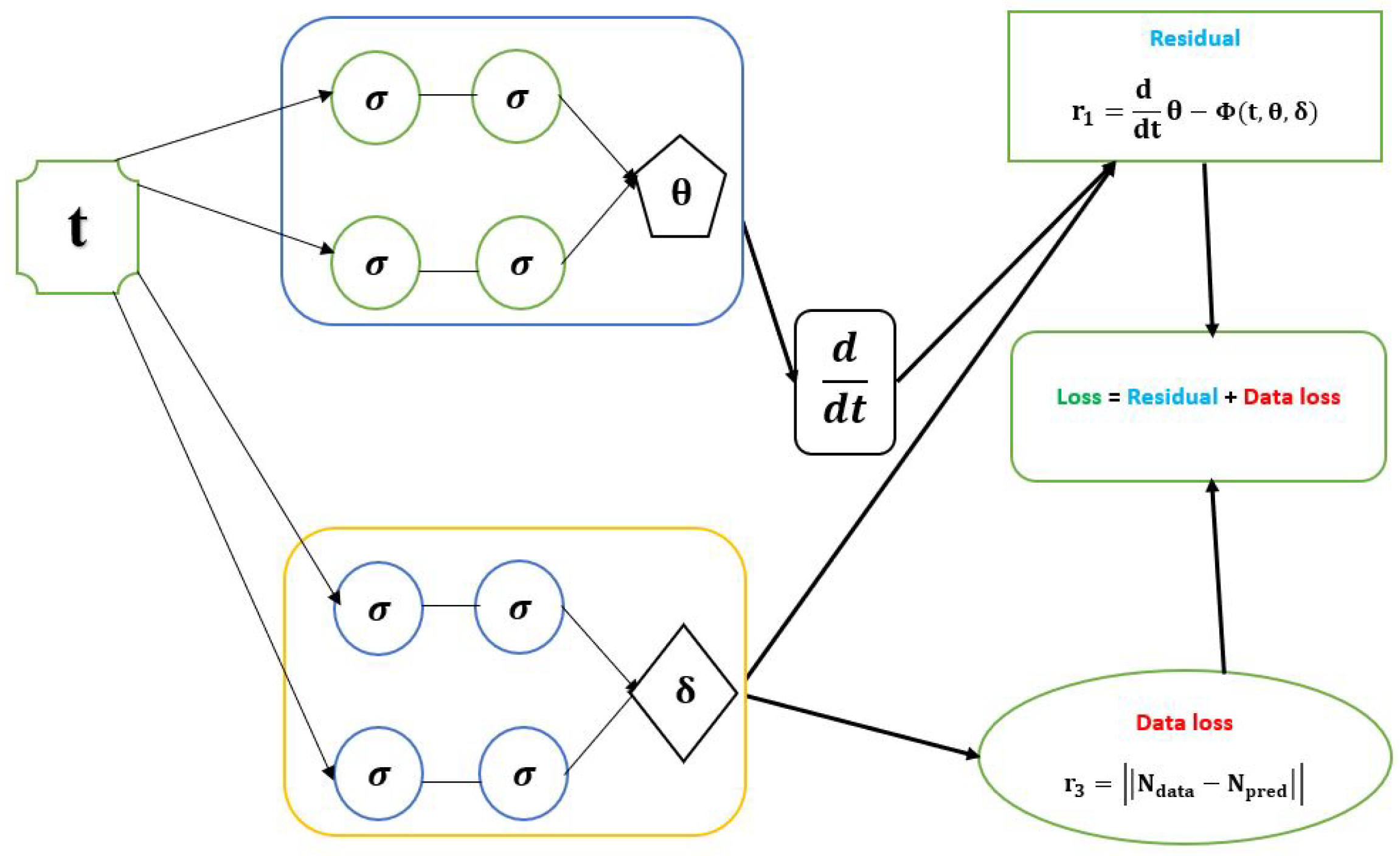
Figure 1.
Schematic diagram of the PINN with the parameters of a dynamical system of ODE model.
Figure 1.
Schematic diagram of the PINN with the parameters of a dynamical system of ODE model.
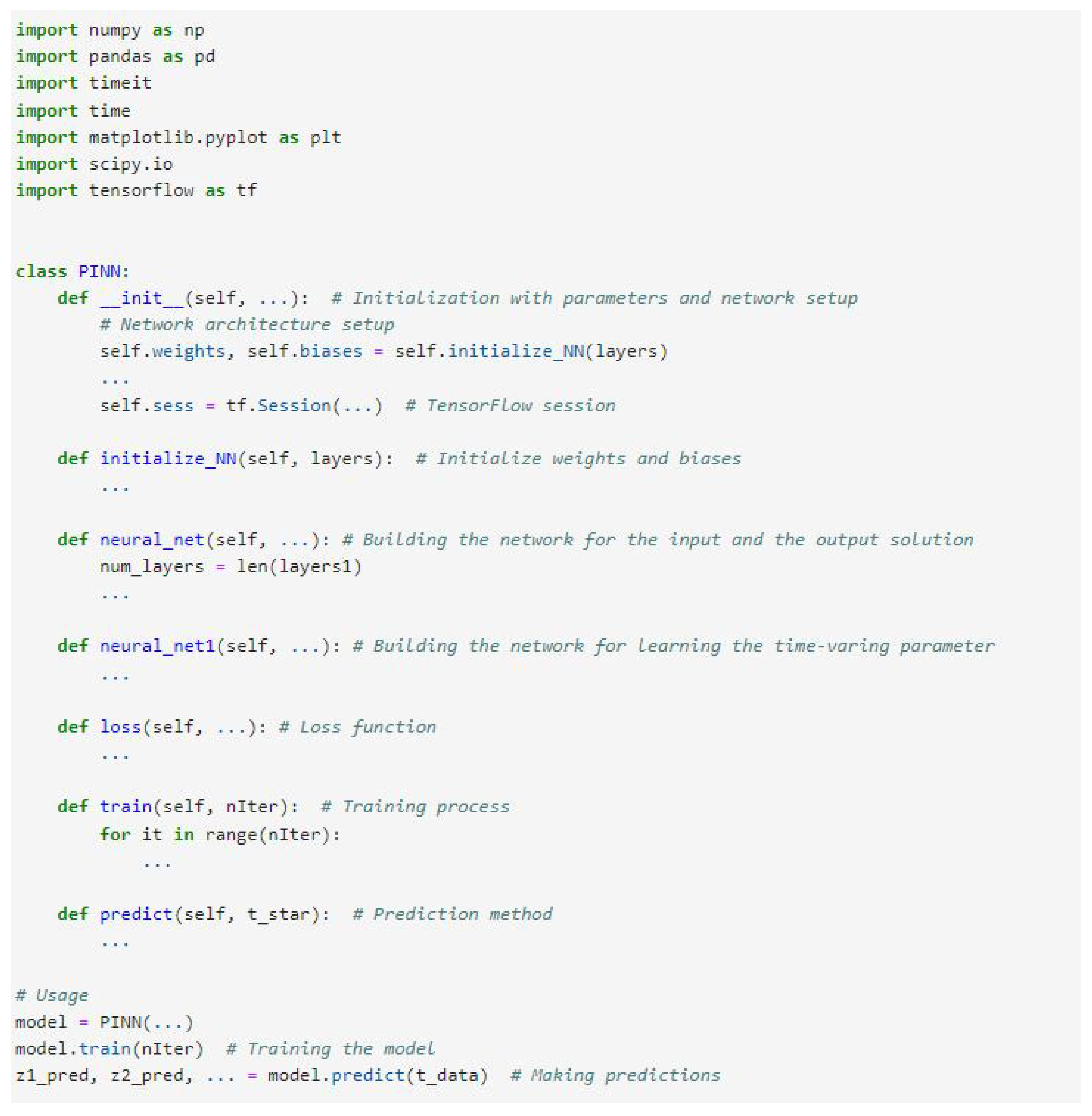
Figure 2.
PINN source code.
Figure 2.
PINN source code.
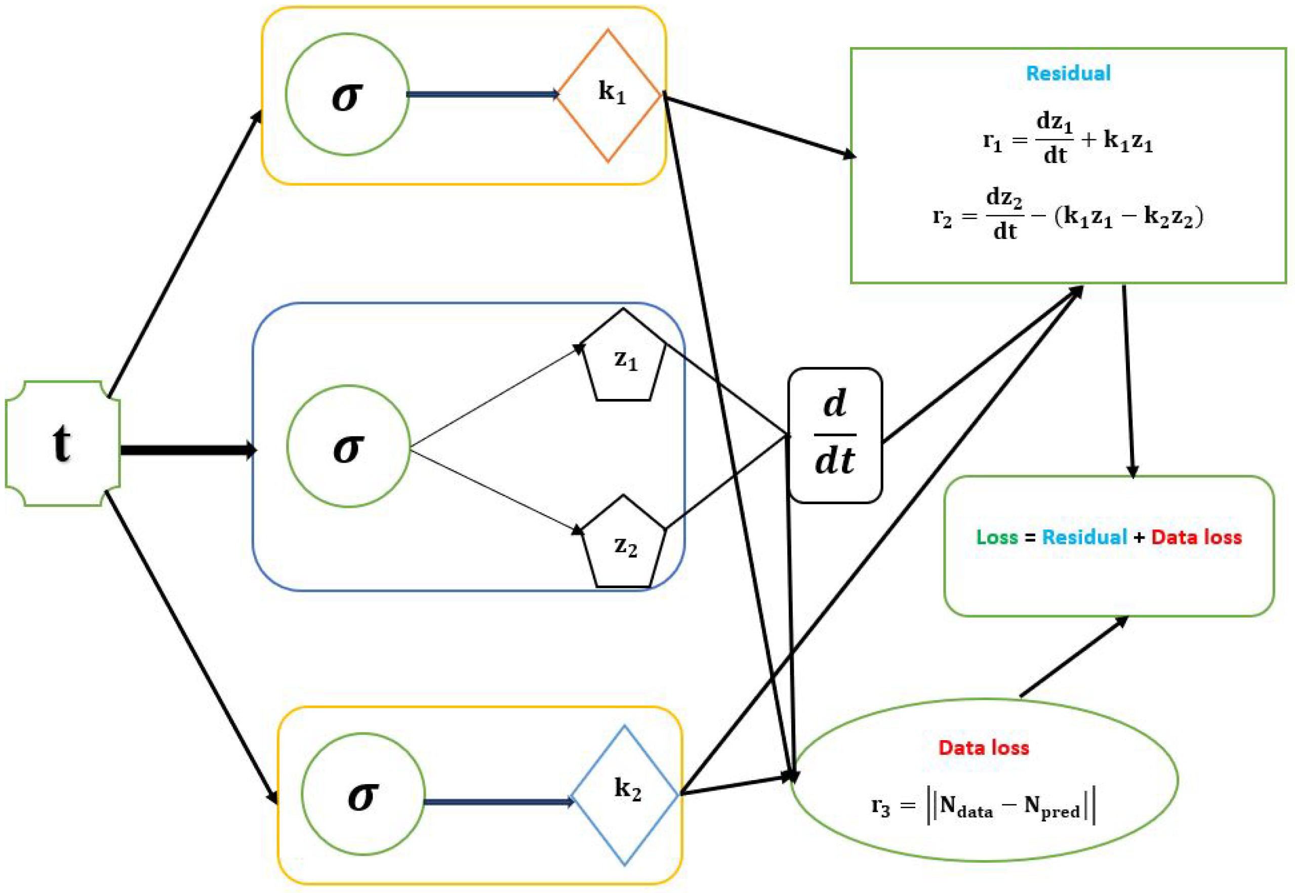
Figure 3.
Schematic diagram of the PINN with the parameters of first-order irreversible chain reactions model.
Figure 3.
Schematic diagram of the PINN with the parameters of first-order irreversible chain reactions model.
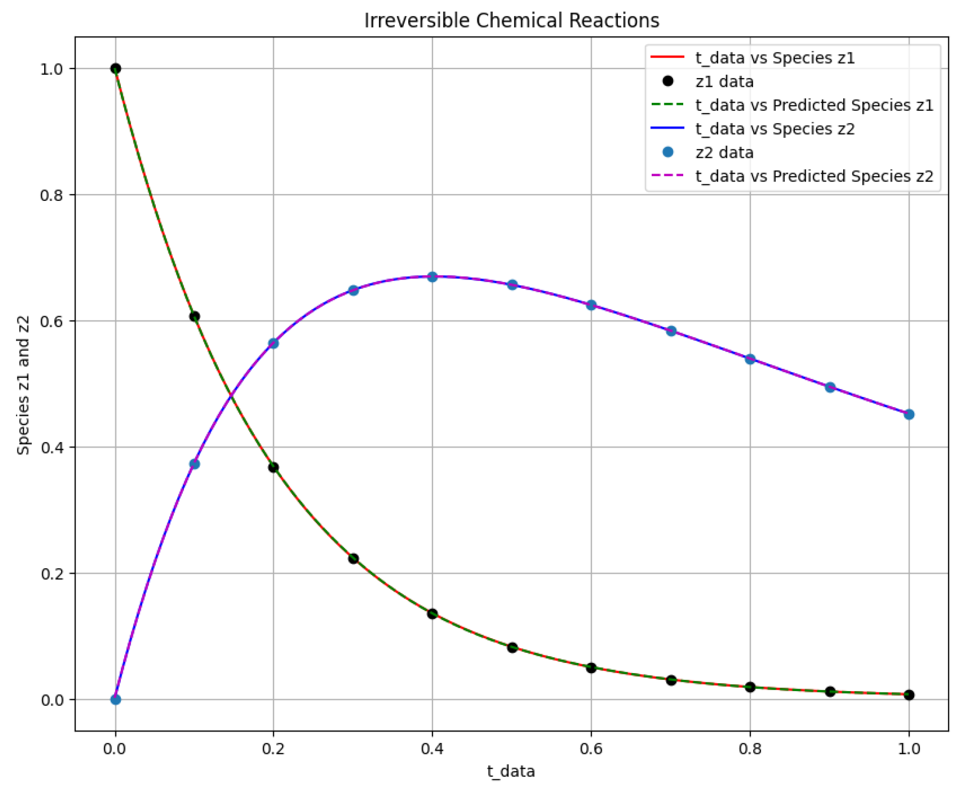
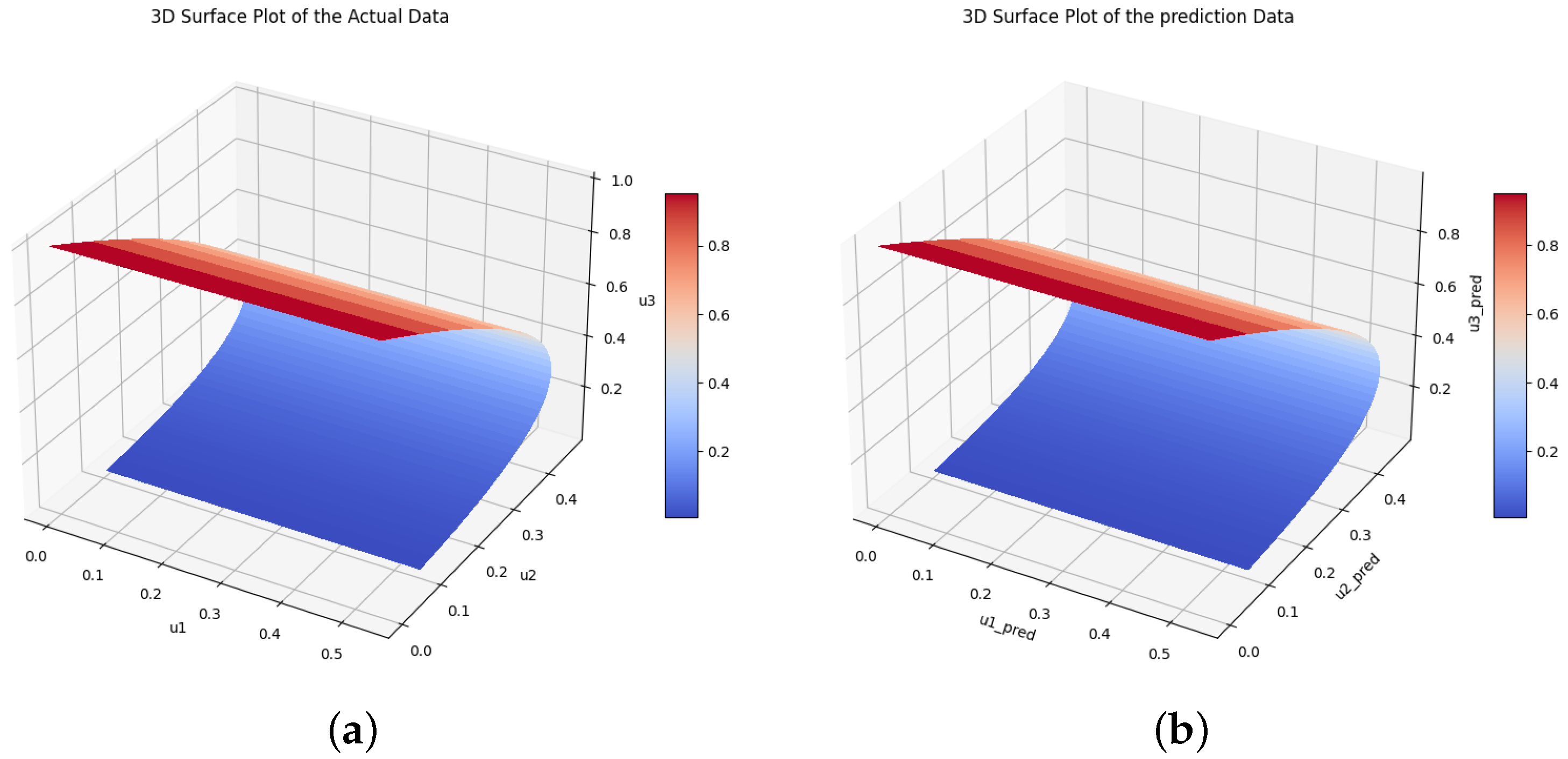
Figure 4.
The first-order irreversible chain reactions solution of the actual output of species against and the predicted output of species against .
Figure 4.
The first-order irreversible chain reactions solution of the actual output of species against and the predicted output of species against .
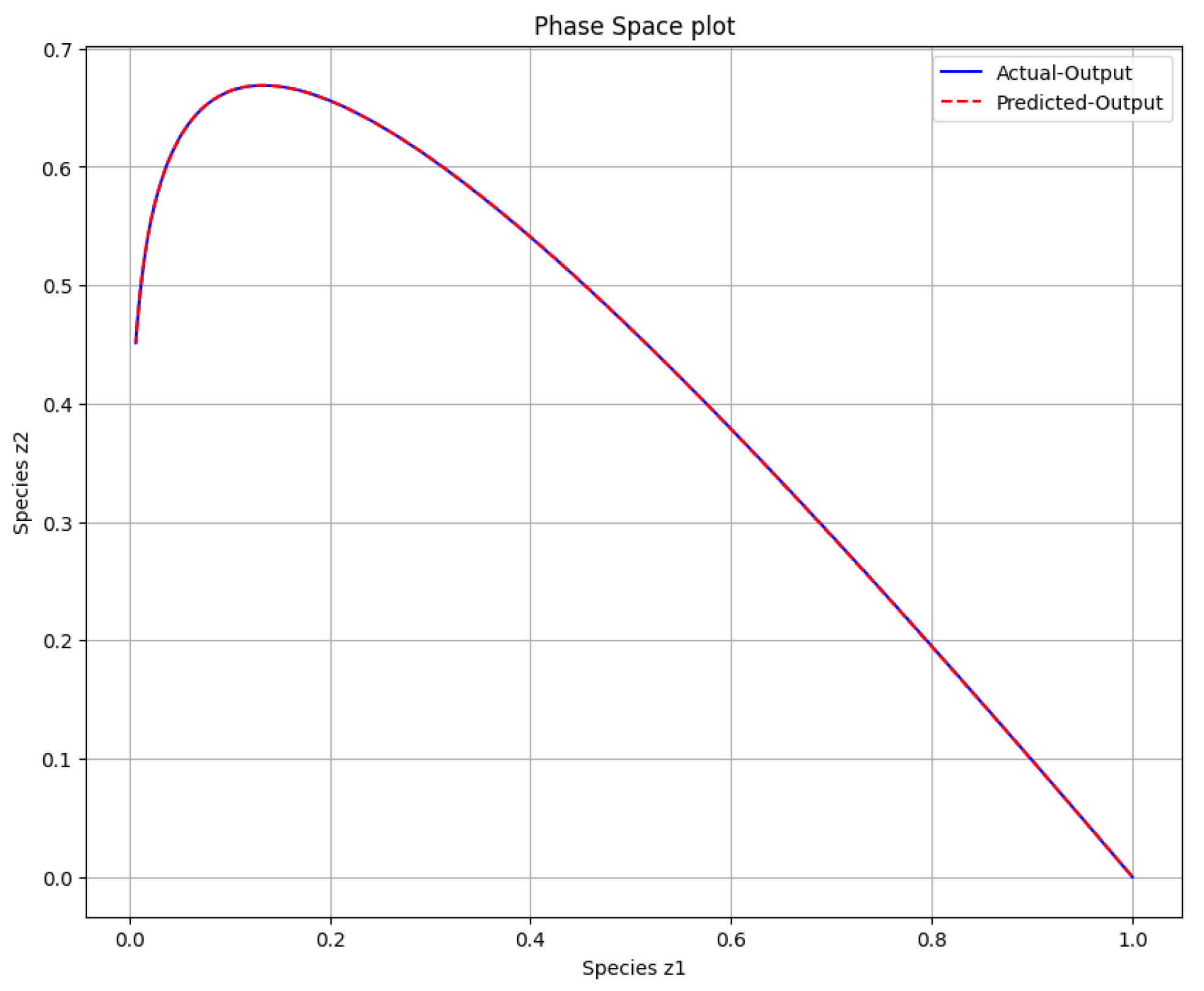
Figure 5.
The phase space plot of the actual output of species against species and the predicted output of species against species .
Figure 5.
The phase space plot of the actual output of species against species and the predicted output of species against species .
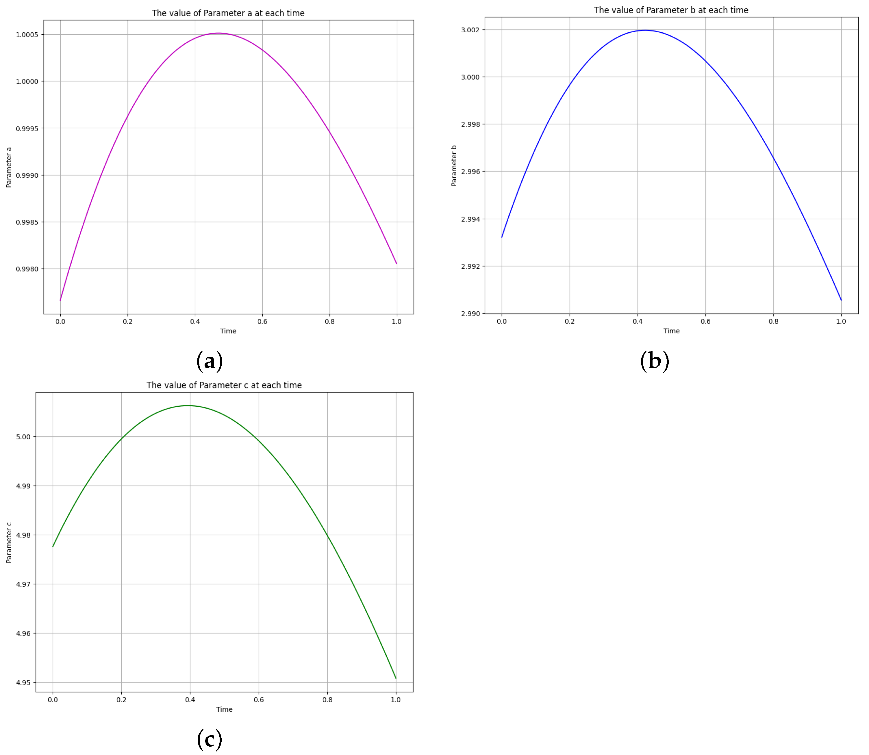
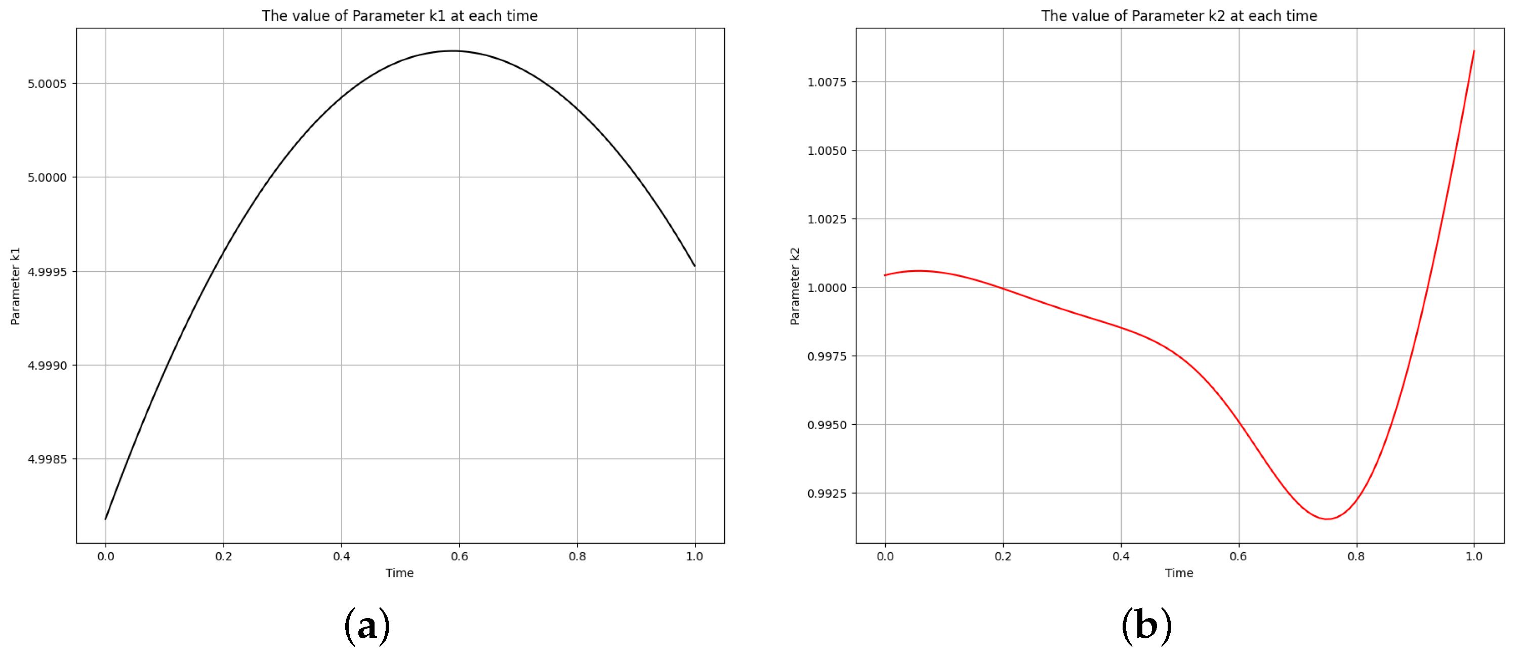
Figure 6.
The learned time-varying parameter values of the first-order irreversible chain reactions model. (a) Time-varying parameter . (b) Time-varying parameter .
Figure 6.
The learned time-varying parameter values of the first-order irreversible chain reactions model. (a) Time-varying parameter . (b) Time-varying parameter .
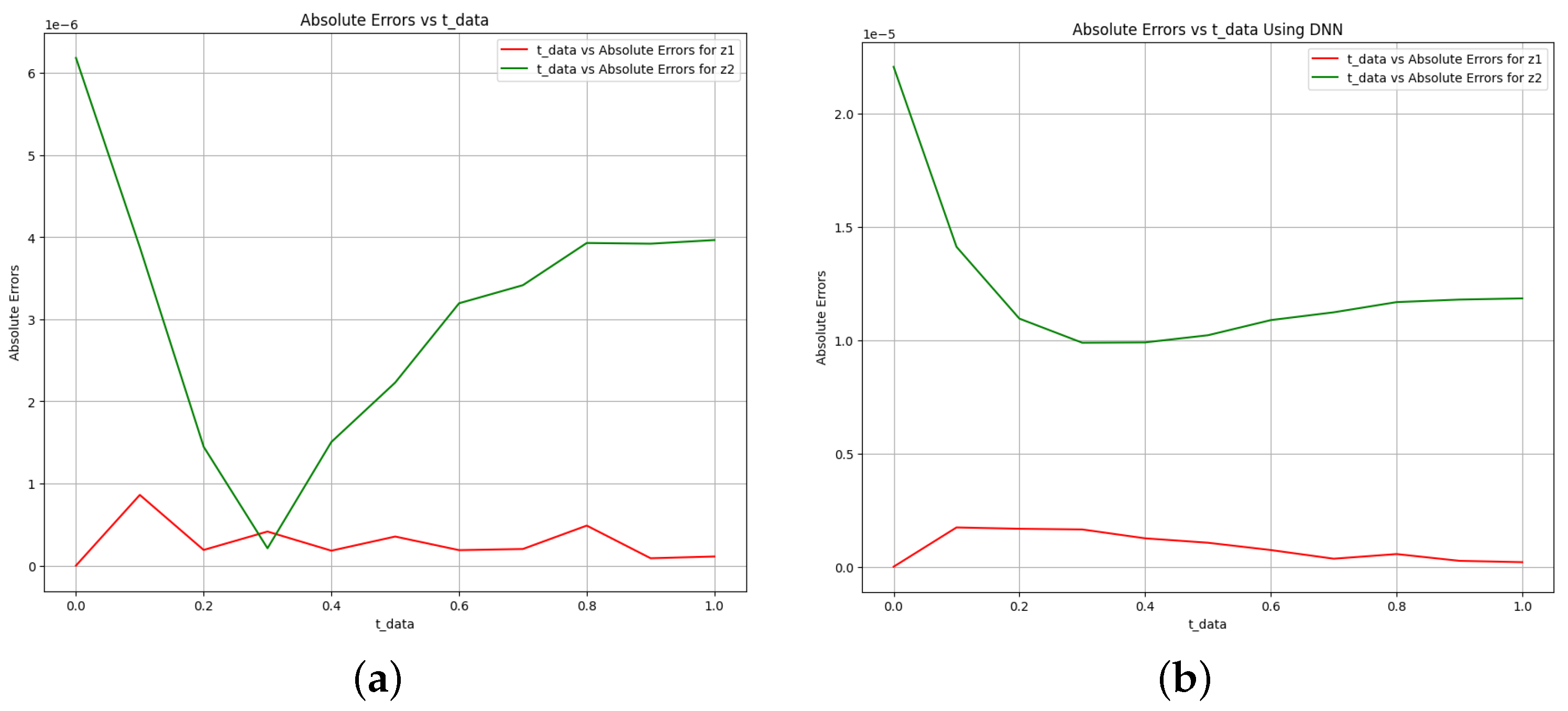
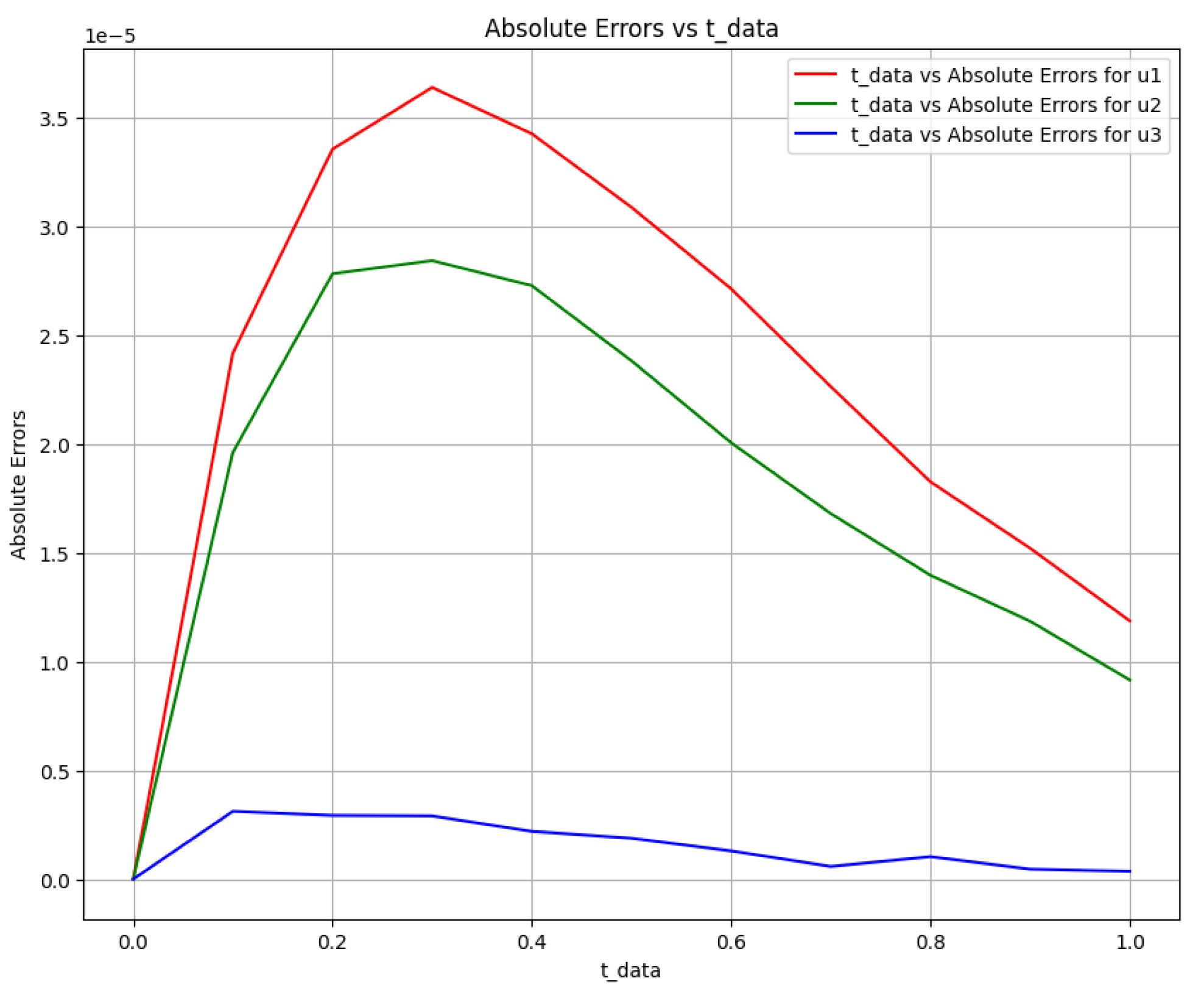
Figure 7.
Absolute error plot between the data, PINN solution, and DNN solution. (a) Absolute error plot using PINN. (b) Absolute error plot using DNN.
Figure 7.
Absolute error plot between the data, PINN solution, and DNN solution. (a) Absolute error plot using PINN. (b) Absolute error plot using DNN.
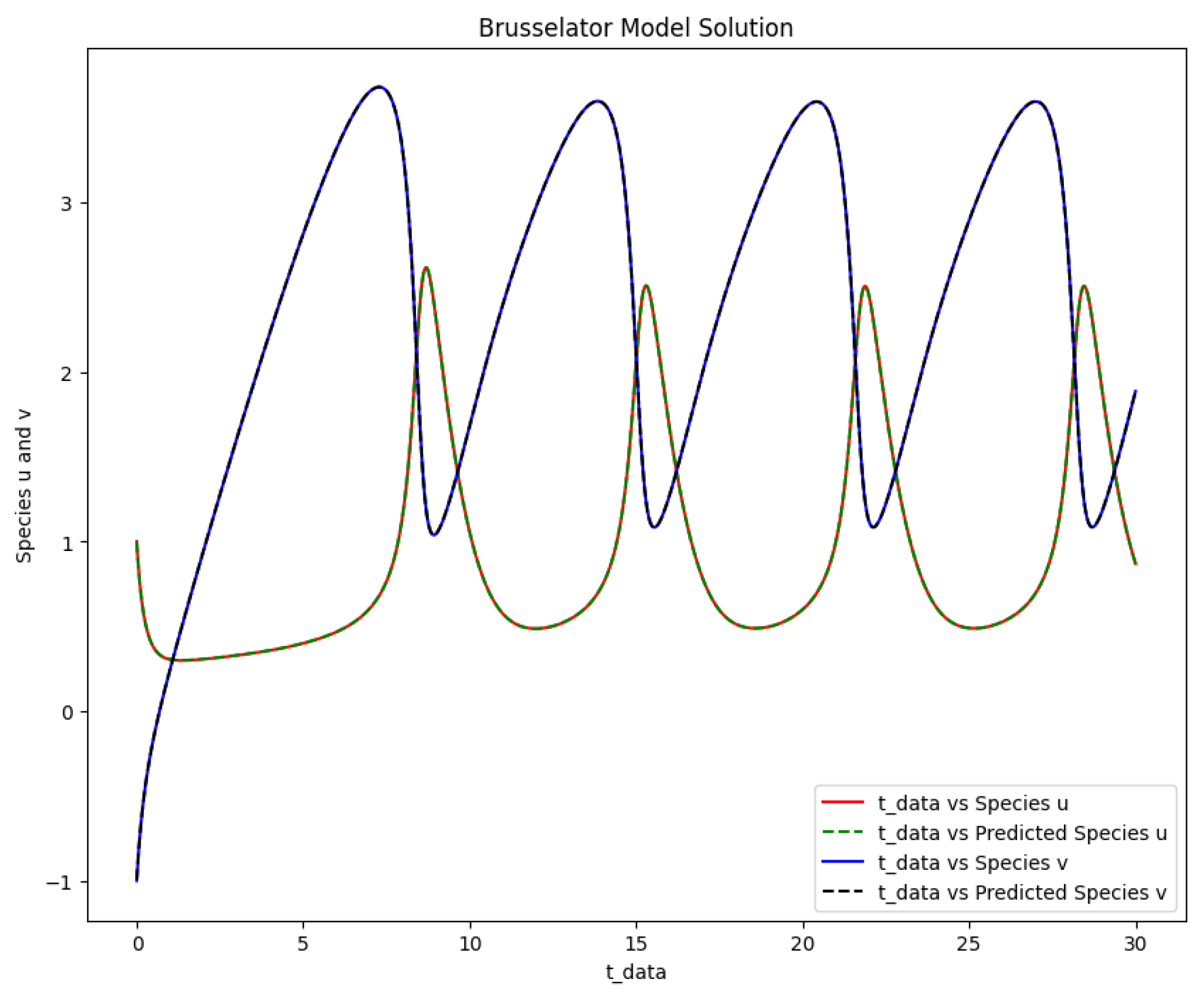
Figure 8.
The Brusselator model solution of the actual output of species u,v against and the predicted output of species u,v against .
Figure 8.
The Brusselator model solution of the actual output of species u,v against and the predicted output of species u,v against .
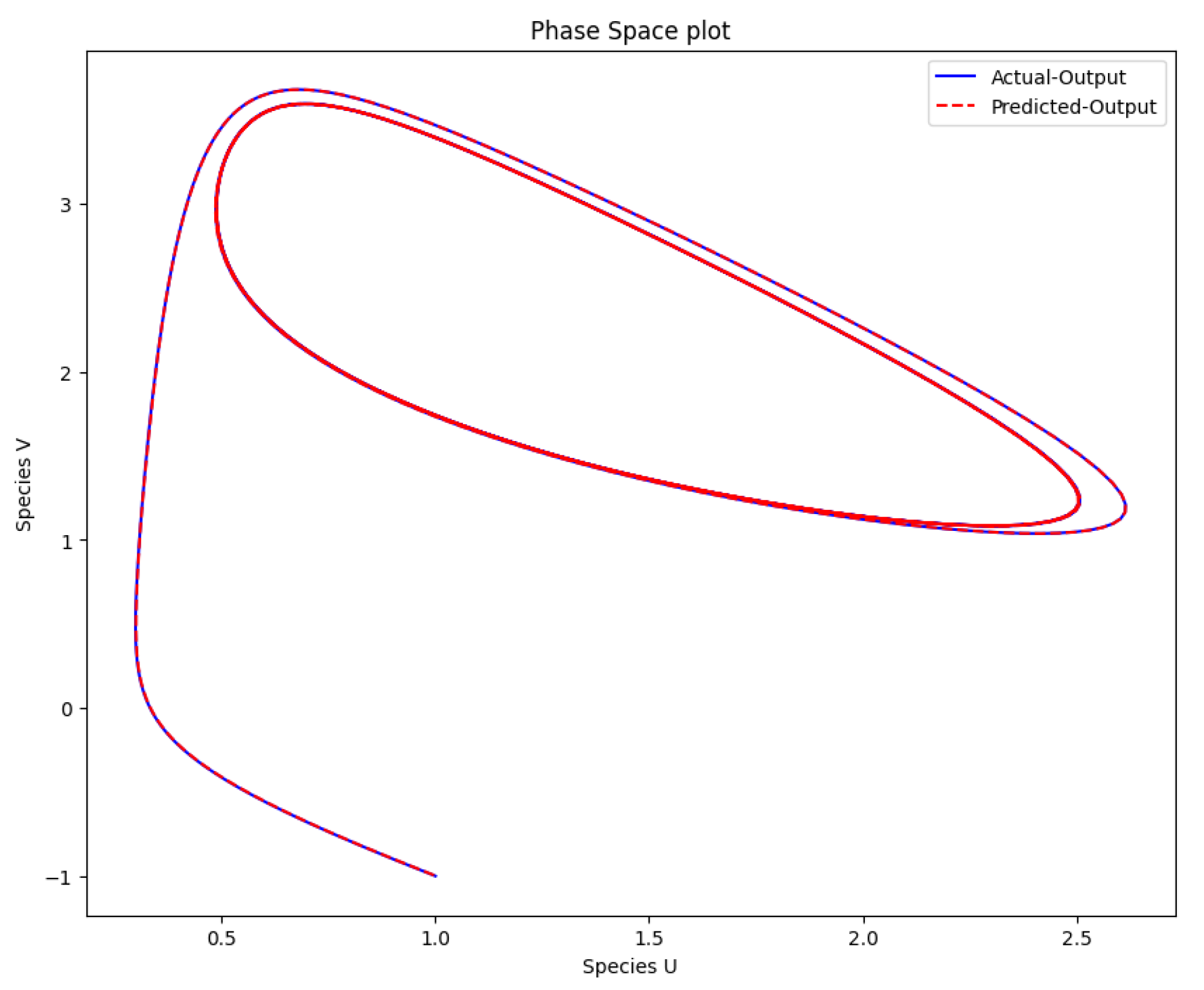
Figure 9.
The phase space plot of the actual output of species u against species v and the predicted output of species u against species v.
Figure 9.
The phase space plot of the actual output of species u against species v and the predicted output of species u against species v.
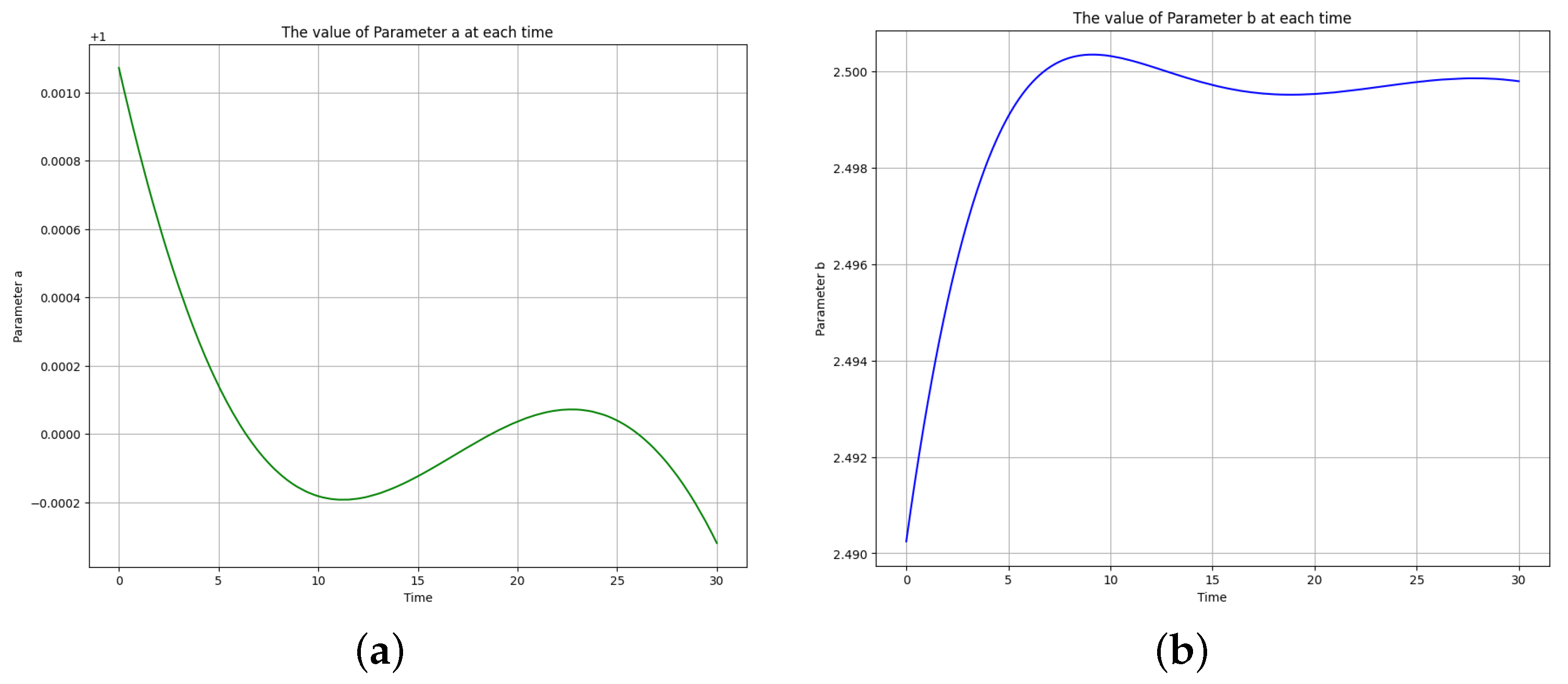
Figure 10.
The learned time-varying parameter values of the Brusselator model. (a) Time-varying parameter a. (b) Time-varying parameter b.
Figure 10.
The learned time-varying parameter values of the Brusselator model. (a) Time-varying parameter a. (b) Time-varying parameter b.
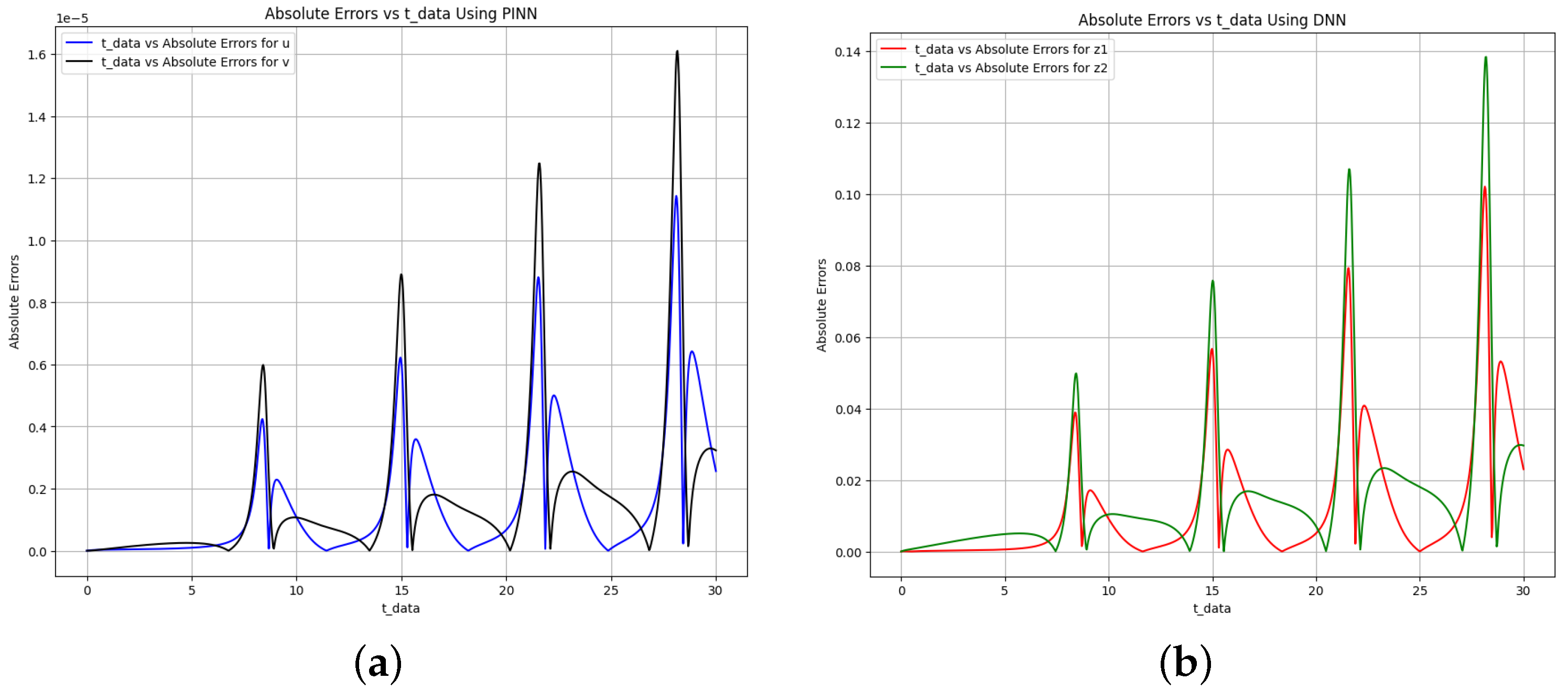
Figure 11.
Absolute error plot between the data, PINN solution, and DNN solution for the Brusselator model. (a) Absolute error plot using PINN. (b) Absolute error plot using DNN.
Figure 11.
Absolute error plot between the data, PINN solution, and DNN solution for the Brusselator model. (a) Absolute error plot using PINN. (b) Absolute error plot using DNN.
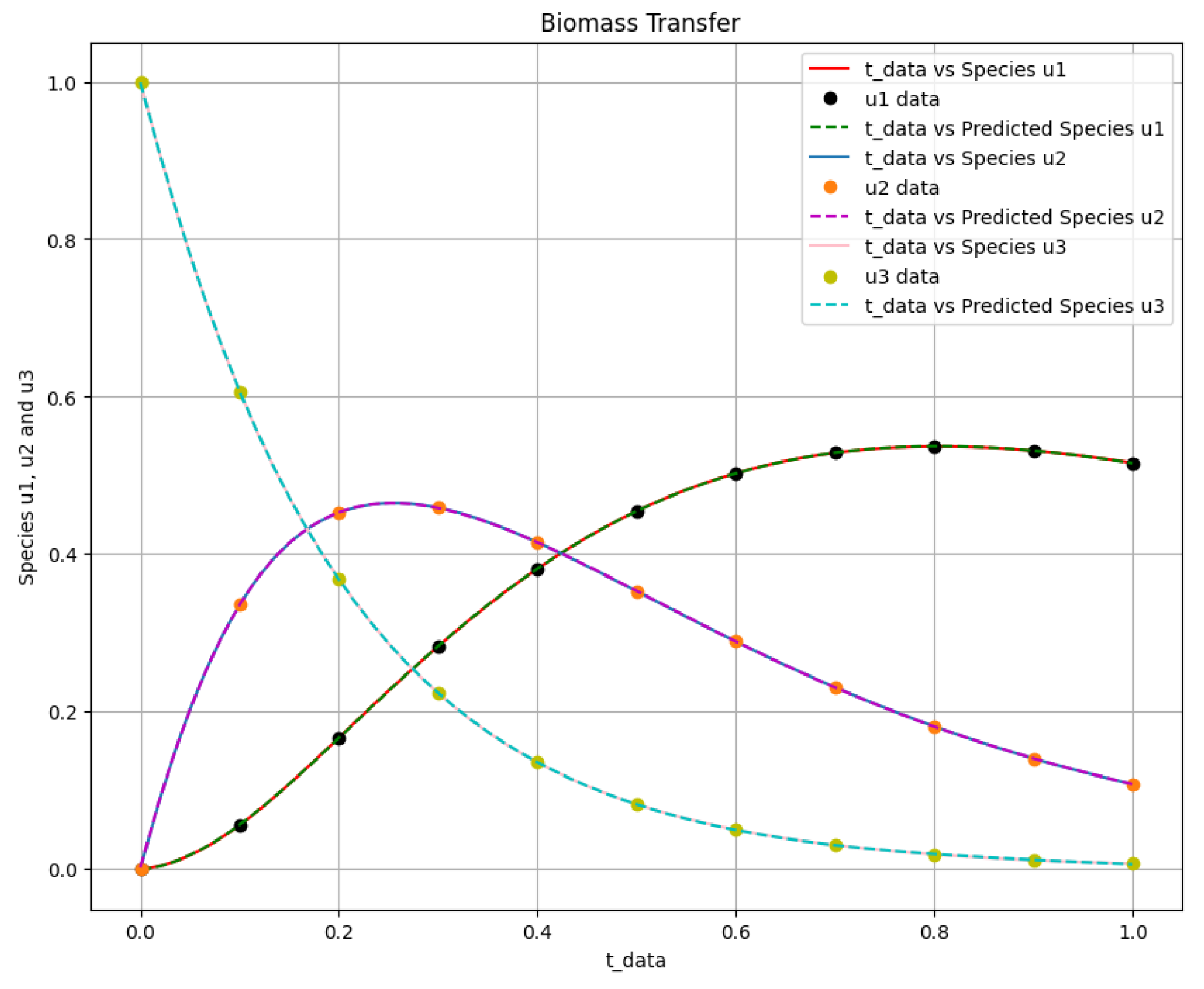
Figure 12.
The biomass transfer exact solution and the predicted output of species against .
Figure 12.
The biomass transfer exact solution and the predicted output of species against .
Figure 13.
The true and the predicted values of species and . (a) The true values of species U. (b) The predicted values of species U.
Figure 13.
The true and the predicted values of species and . (a) The true values of species U. (b) The predicted values of species U.
Figure 14.
The learned time-varying parameter values of the biomass transfer model. (a) Time-varying parameter a. (b) Time-varying parameter b. (c) Time-varying parameter c.
Figure 14.
The learned time-varying parameter values of the biomass transfer model. (a) Time-varying parameter a. (b) Time-varying parameter b. (c) Time-varying parameter c.
Figure 15.
Absolute error plot between the data and PINN solution.
Figure 15.
Absolute error plot between the data and PINN solution.
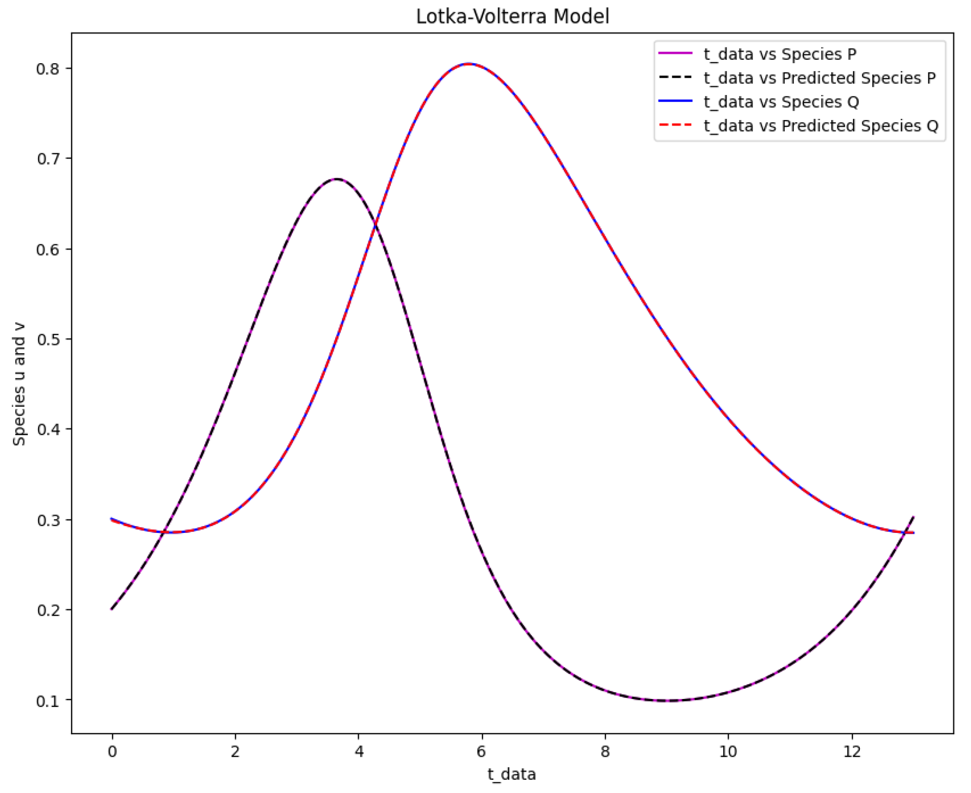
Figure 16.
The Lotka-Volterra model solution for the real output of species P and Q against time data and the predicted output of species P and Q against time data.
Figure 16.
The Lotka-Volterra model solution for the real output of species P and Q against time data and the predicted output of species P and Q against time data.
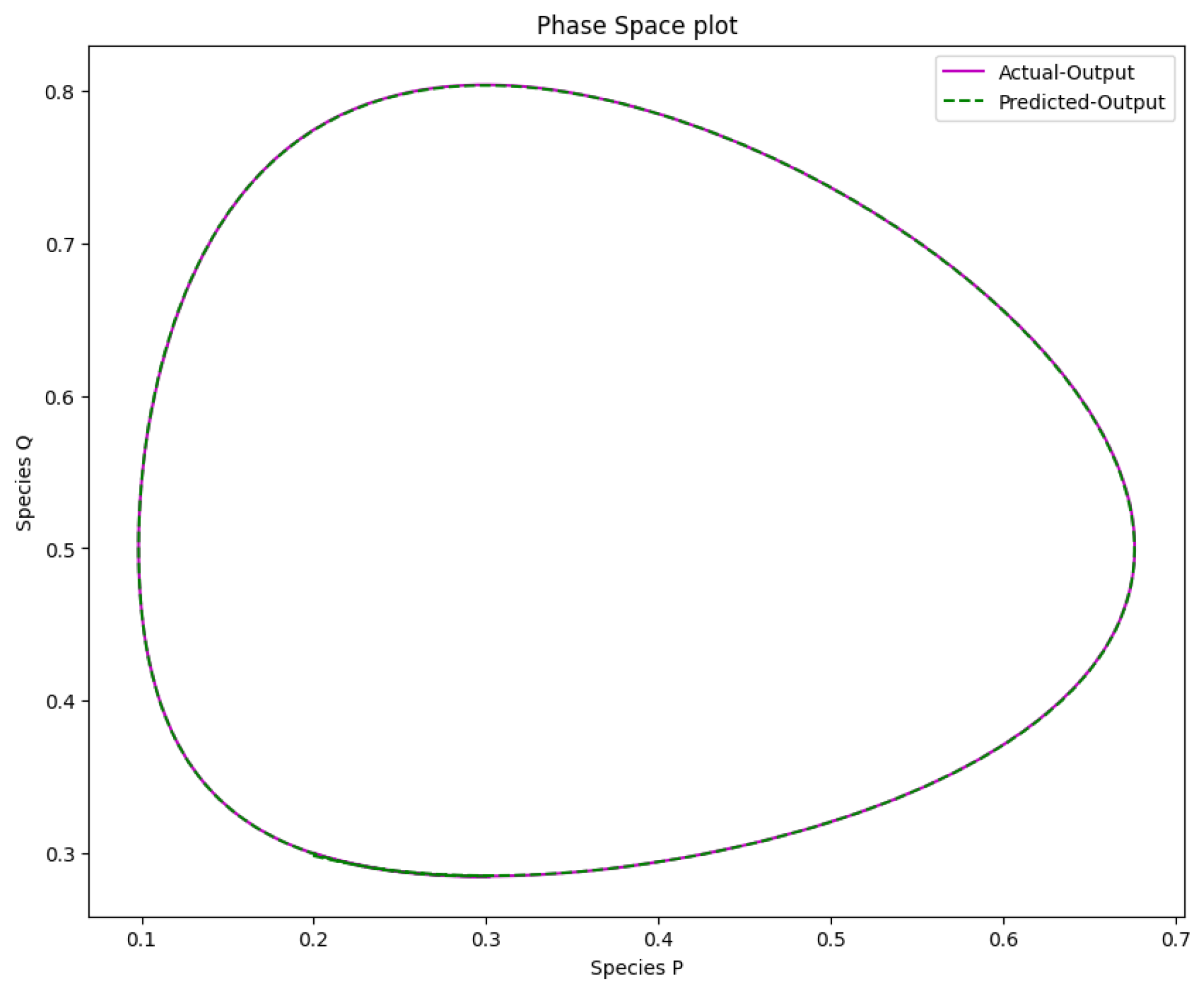
Figure 17.
The phase space plot of the actual output of species P against species Q and the predicted output of species P against species Q of the Lotka-Volterra model.
Figure 17.
The phase space plot of the actual output of species P against species Q and the predicted output of species P against species Q of the Lotka-Volterra model.
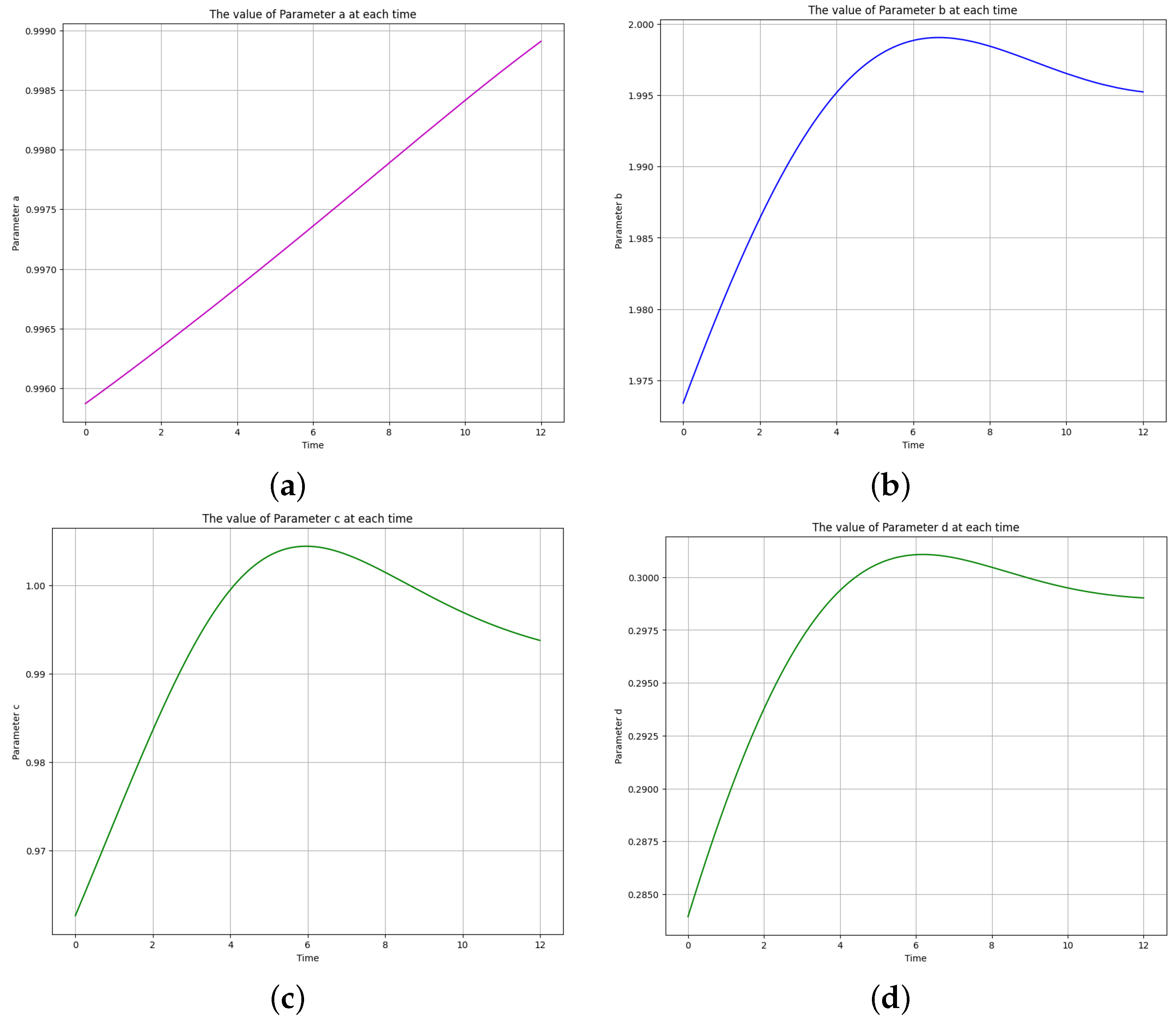
Figure 18.
The learned time-varying parameter values of the Lotka-Volterra model. (a) Time-varying parameter a. (b) Time-varying parameter b. (c) Time-varying parameter c. (d) Time-varying parameter d.
Figure 18.
The learned time-varying parameter values of the Lotka-Volterra model. (a) Time-varying parameter a. (b) Time-varying parameter b. (c) Time-varying parameter c. (d) Time-varying parameter d.
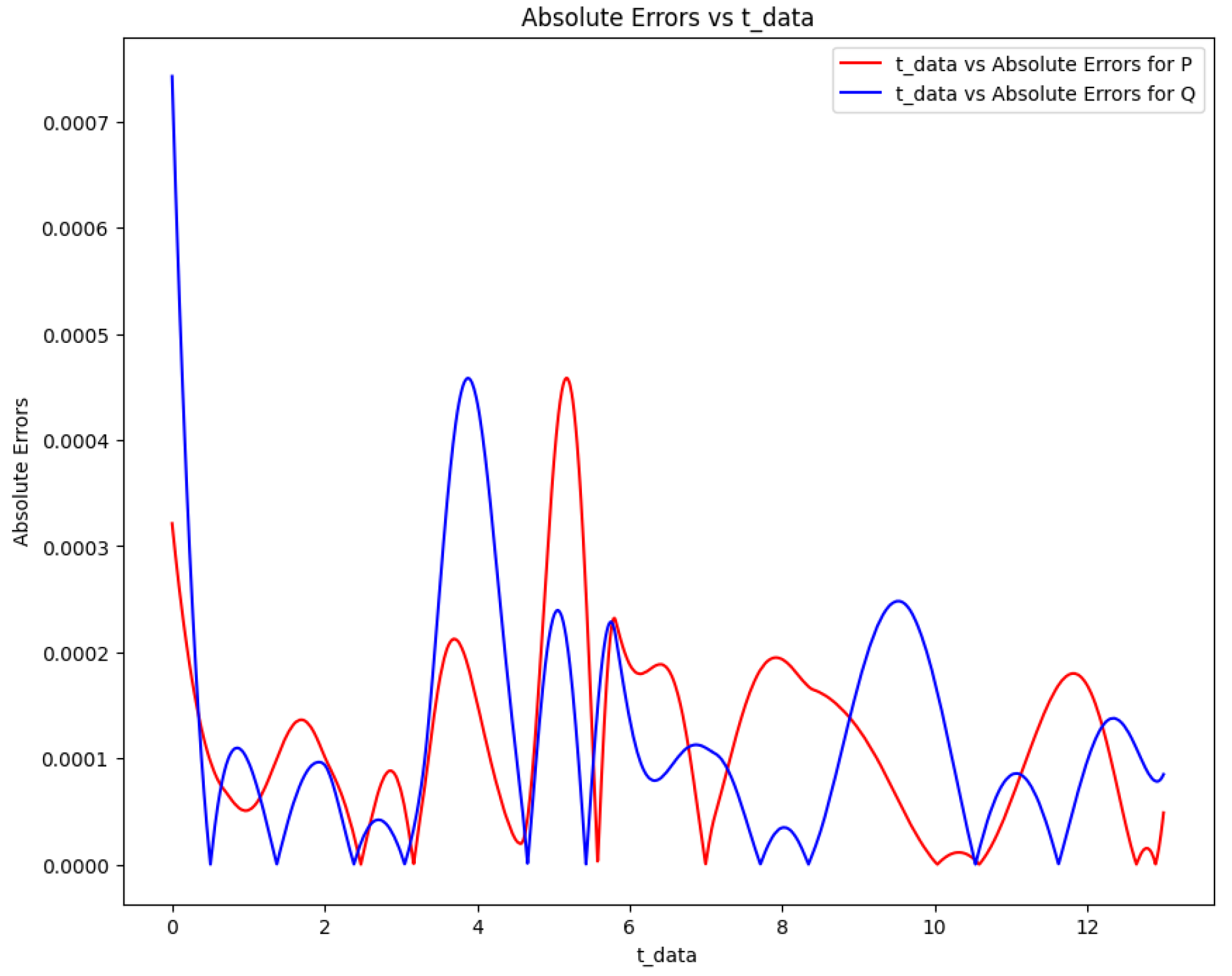
Figure 19.
Absolute error plot between the data and PINN solution of the Lotka-Volterra model.
Figure 19.
Absolute error plot between the data and PINN solution of the Lotka-Volterra model.
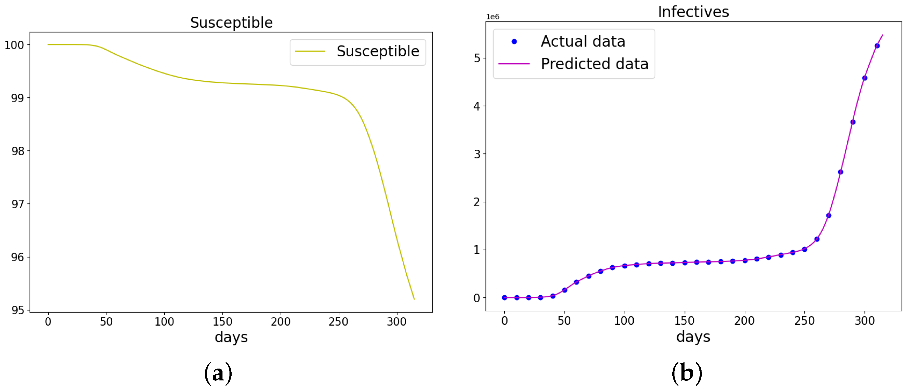
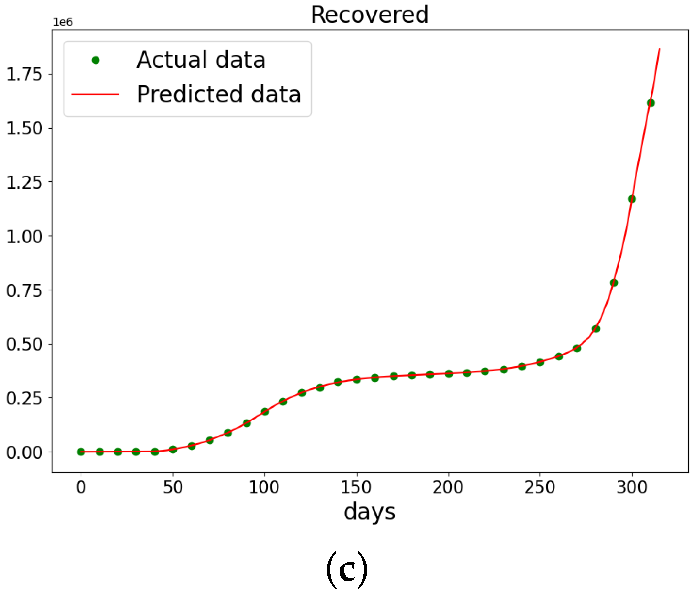
Figure 20.
The data and the learned SIR model using PINN Algorithm 5 on COVID-19 data. (a) The susceptible graph. (b) The data and the learned infectives. (c) The data and the learned recovered population.
Figure 20.
The data and the learned SIR model using PINN Algorithm 5 on COVID-19 data. (a) The susceptible graph. (b) The data and the learned infectives. (c) The data and the learned recovered population.
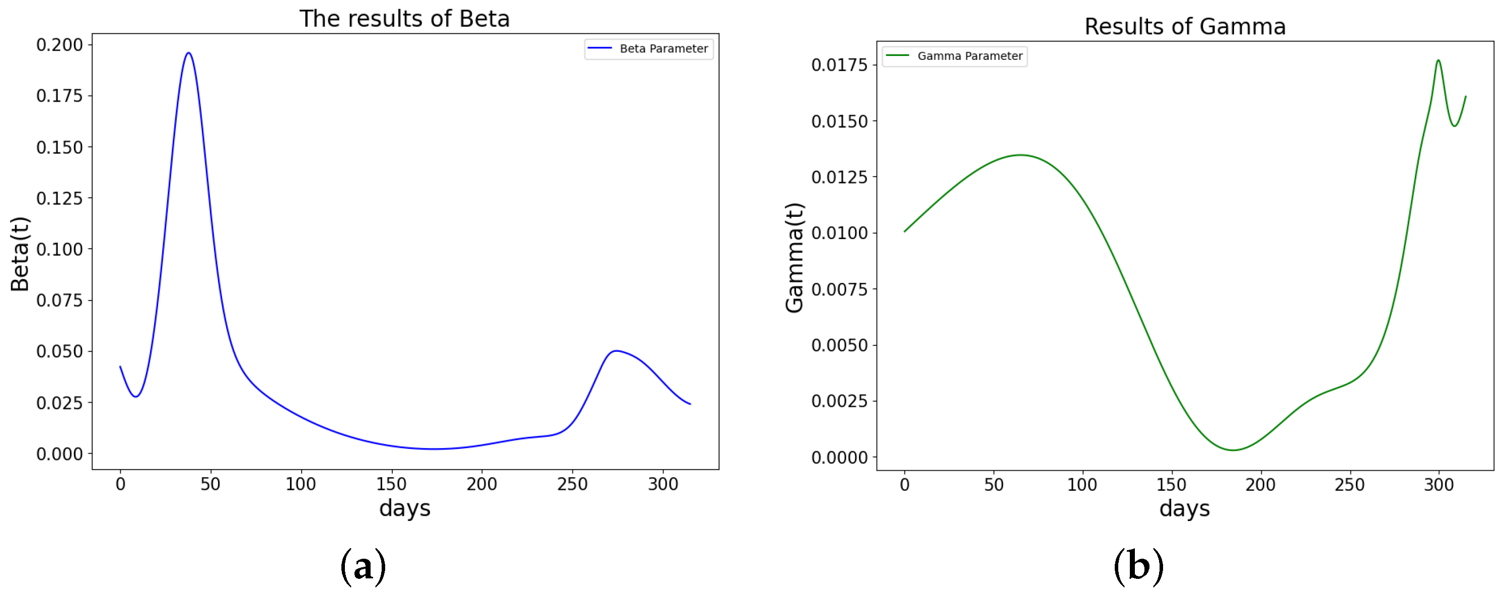
Figure 21.
The learned parameters of SIR model using PINN Algorithm 5 on COVID-19 data. (a) The learned . (b) The learned .
Figure 21.
The learned parameters of SIR model using PINN Algorithm 5 on COVID-19 data. (a) The learned . (b) The learned .
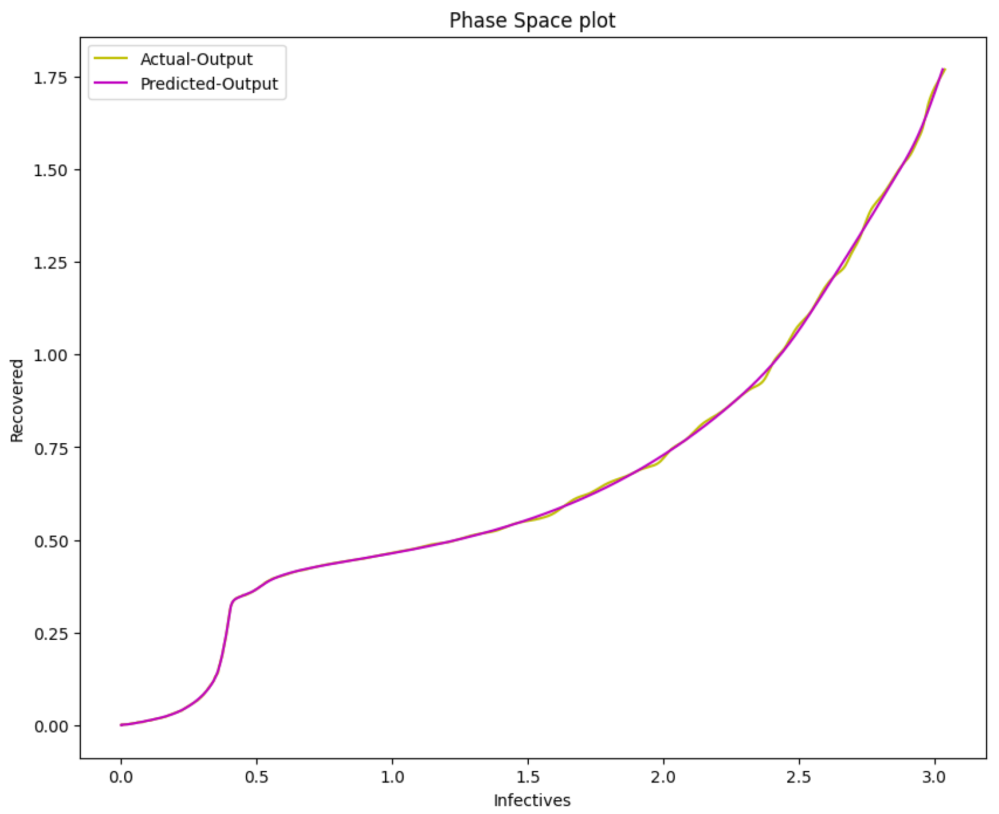
Figure 22.
The phase space plot of the actual output of I against R and the predicted output of I against R of the SIR model from the COVID-19 data.
Figure 22.
The phase space plot of the actual output of I against R and the predicted output of I against R of the SIR model from the COVID-19 data.
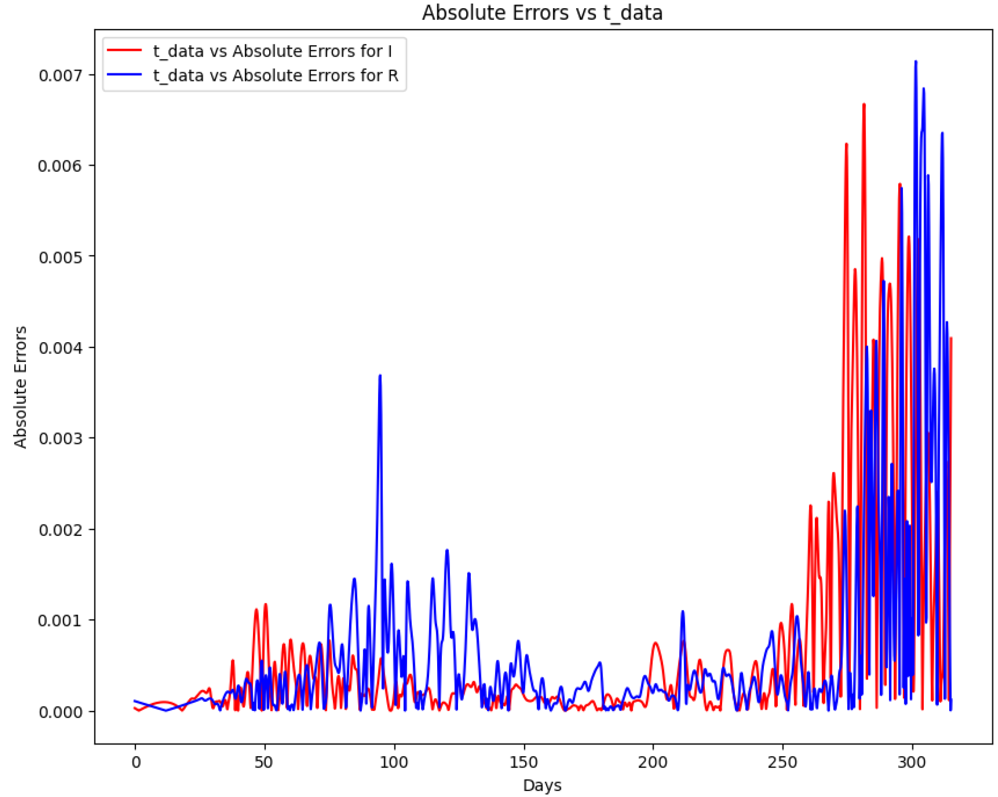
Figure 23.
Absolute error plot between the COVID-19 data and the PINN solution of the SIR model.
Figure 23.
Absolute error plot between the COVID-19 data and the PINN solution of the SIR model.
Table 1.
Observed values of and at different time points.
Table 1.
Observed values of and at different time points.
| t | | |
|---|
| 0.0 | 1.000000 | 0.000000 |
| 0.1 | 0.606531 | 0.372883 |
| 0.2 | 0.367879 | 0.563564 |
| 0.3 | 0.223130 | 0.647110 |
| 0.4 | 0.135335 | 0.668731 |
| 0.5 | 0.082085 | 0.655557 |
| 0.6 | 0.049787 | 0.623781 |
| 0.7 | 0.030197 | 0.582985 |
| 0.8 | 0.018316 | 0.538767 |
| 0.9 | 0.011109 | 0.494326 |
| 1.0 | 0.006738 | 0.451427 |
Table 2.
Comparison of the two approaches using PINN.
Table 2.
Comparison of the two approaches using PINN.
| | | |
|---|
| True Values | 5.0 | 1.0 |
| Approach 1 | 5.0000086 | 0.99999505 |
| Error of Approach 1 | 0.0000086 | 0.00000495 |
| Approach 2 | 5.0005193 | 1.0001917 |
| Error of Approach 1 | 0.0005193 | 0.0001917 |
| | | |
| MAE of Approach 1 | 2.7979 | 3.0801 |
| MAE of Approach 2 | 1.7826 | 3.7310 |
| MSE of Approach 1 | 1.3095 | 1.1916 |
| MSE of Approach 2 | 4.8358 | 2.0368 |
| RMSE of Approach 1 | 3.6187 | 3.4519 |
| RMSE of Approach 2 | 2.1991 | 4.5131 |
Table 3.
Comparison of obtained results using PINN vs. DNN through the approaches described in Scenario 1. The table demonstrates a significant 67.7% improvement in computational efficiency when employing PINNs compared to DNNs, highlighting the enhanced performance and time-saving capabilities of PINNs in dynamic system modeling.
| | True Values | PINN | DNN | Epochs | CPU Using PINN | CPU Using DNN |
|---|
| 5.0 | 5.0000086 | 5.0000643 | | | |
| | | | | 90,000 | 40s | 124s |
| 1.0 | 0.99999505 | 1.0000190 | | | |
Table 4.
Comparison of obtained error results using PINN vs. DNN. This table presents a detailed analysis of the error metrics for both PINN and DNN models across two variables, and . The results highlight the superior accuracy of PINNs, as evidenced by significantly lower error values across all metrics compared to DNNs, underscoring the effectiveness of PINNs in dynamic system modeling.
| Error Metrics | | | | |
|---|
| 2.7979 | 2.1615 | 3.0801 | 2.3330 |
| 1.3095 | 7.0444 | 1.1916 | 5.6775 |
| 3.6187 | 2.6541 | 3.4519 | 2.3827 |
Table 5.
Comparison of PINN vs. DNN based on shallow vs. deep layers through the approaches described in Scenario 1. This table details the accuracy of parameter estimation ( and ) and computational performance across various network depths. Notably, it showcases the increasing computational efficiency of PINNs over DNNs, with improvements of , and for different layer configurations. These findings emphasize the enhanced efficiency and adaptability of PINNs in handling complex dynamical systems, especially in deeper network architectures.
| Layers | Neurons | (PINN) | (DNN) | (PINN) | (DNN) | Epochs | CPU PINN | CPU DNN |
|---|
| 1 | 40 | 4.99815 | 4.9925046 | 1.0002131 | 0.9969400 | 21378 | 10s | 30s |
| 2 | 40, 40 | 5.0000534 | 4.9999063 | 1.00021 | 1.0000036 | 24358 | 13s | 33s |
| 3 | 40, 40, 40 | 4.999991 | 5.0050346 | 0.9999847 | 1.0018185 | 16021 | 9s | 24s |
Table 6.
The optimal parameter estimation and the error metrics using PINN.
Table 6.
The optimal parameter estimation and the error metrics using PINN.
| | a | b |
|---|
| True Values | 1.0 | 2.5 |
| Approach 2 | 1.0000001 | 2.5 |
| Error of Approach 2 | 0.0000001 | 0.0000 |
| | u | v |
| MAE of Approach 2 | 1.5247 | 1.7520 |
| MSE of Approach 2 | 6.5662 | 9.5430 |
| RMSE of Approach 2 | 2.5625 | 3.0892 |
Table 7.
Comparison of obtained results using PINN vs. DNN through the approaches described in Scenario 1. This table illustrates the accuracy in parameter estimation and the significant computational efficiency improvement of 88.7% with PINNs over DNNs, highlighting the robustness and speed of PINNs in complex system modeling.
| | True Values | PINN | DNN | Epochs | CPU Using PINN | CPU Using DNN |
|---|
| a | 1.0 | 1.0000001 | 1.0038480 | | | |
| | | | | 50,000 | 111s | 982s |
| b | 2.5 | 2.5 | 2.5088659 | | | |
Table 8.
Comparison of obtained error results using PINN vs. DNN.
Table 8.
Comparison of obtained error results using PINN vs. DNN.
| Error Metrics | | | | |
|---|
| 1.5247 | 3.6030 | 1.7520 | 4.5508 |
| 6.5662 | 3.8405 | 9.5430 | 5.4941 |
| 2.5624 | 6.1972 | 3.0891 | 7.4122 |
Table 9.
Analysis of the Brusselator model using different epochs.
Table 9.
Analysis of the Brusselator model using different epochs.
| Epochs | Loss | Error u | Error v |
|---|
| 50,000 | 2.7514 | 7.9001 | 5.5722 |
| 40,000 | 1.9048 | 1.5938 | 3.3815 |
| 30,000 | 1.5272 | 2.8571 | 5.4818 |
Table 10.
Observed values of and at different time points.
Table 10.
Observed values of and at different time points.
| t | | | |
|---|
| 0.0 | 0.000000 | 0.000000 | 1.000000 |
| 0.1 | 0.055747 | 0.335719 | 0.606531 |
| 0.2 | 0.166850 | 0.452330 | 0.367879 |
| 0.3 | 0.282767 | 0.458599 | 0.223130 |
| 0.4 | 0.381125 | 0.414647 | 0.135335 |
| 0.5 | 0.454416 | 0.352613 | 0.082085 |
| 0.6 | 0.502502 | 0.288780 | 0.049787 |
| 0.7 | 0.528506 | 0.230648 | 0.030197 |
| 0.8 | 0.536641 | 0.181006 | 0.018316 |
| 0.9 | 0.531127 | 0.140241 | 0.011109 |
| 1.0 | 0.515706 | 0.107623 | 0.006738 |
Table 11.
Comparison of the two approaches using PINN.
Table 11.
Comparison of the two approaches using PINN.
| | a | b | c |
|---|
| True Values | 1.0 | 3.0 | 5.0 |
| Approach 1 | 0.99999785 | 2.999931 | 5.000046 |
| Error of Approach 1 | 0.00000215 | 0.000069 | 0.000046 |
| Approach 2 | 1.0000874 | 3.0001755 | 5.0010123 |
| Error of Approach 1 | 0.0000874 | 0.0001755 | 0.0010123 |
| | | | |
| MAE of Approach 1 | 2.3118 | 1.8068 | 1.5237 |
| MAE of Approach 2 | 2.1915 | 2.6433 | 3.4797 |
| MSE of Approach 1 | 6.4652 | 3.9821 | 3.5008 |
| MSE of Approach 2 | 6.9882 | 8.9255 | 1.8445 |
| RMSE of Approach 1 | 2.5427 | 1.9955 | 1.8709 |
| RMSE of Approach 2 | 2.6435 | 2.9876 | 4.2948 |
Table 12.
Comparison of obtained results using PINN vs. reported in the literature using DNN.
Table 12.
Comparison of obtained results using PINN vs. reported in the literature using DNN.
| | True Values | PINN | DNN [12] | Epochs |
|---|
| a | 1.0 | 0.99999785 | 1.0024 | |
| | | | | 71,800 |
| b | 3.0 | 2.999931 | 3.0026 | |
| | | | | 71,800 |
| c | 5.0 | 5.000046 | 5.0150 | |
Table 13.
Comparison of PINN vs. reported in the literature using DNN [
12] based on shallow vs. deep layers.
Table 13.
Comparison of PINN vs. reported in the literature using DNN [
12] based on shallow vs. deep layers.
| Layers | Neurons | a (PINN) | a (DNN) | b (PINN) | b (DNN) | c (PINN) | c (DNN) | Epochs |
|---|
| 1 | 40 | 1.0000379 | 1.0044 | 3.0000386 | 2.9936 | 5.0002103 | 4.9451 | 20,000 |
| 2 | 40, 40 | 1.0000603 | 1.0051 | 2.9999495 | 3.0125 | 4.9998903 | 5.0515 | 15,107 |
| 3 | 40, 40, 40 | 0.99996376 | 1.0044 | 3.000064 | 2.9936 | 4.999971 | 4.9451 | 9800 |
Table 14.
The parameter estimation of the Lotka-Volterra model.
Table 14.
The parameter estimation of the Lotka-Volterra model.
| | a | b | c | d |
|---|
| True Values | 1.0 | 2.0 | 1.0 | 0.3 |
| Approach 2 | 0.999136 | 1.9990387 | 1.000002 | 0.3 |
| Error of Approach 2 | 0.000864 | 0.0009619 | 0.000002 | 0.00 |
Table 15.
The error metrics of the Lotka-Volterra model.
Table 15.
The error metrics of the Lotka-Volterra model.
| | P | Q |
|---|
| MAE | 2.3452 | 2.4140 |
| MSE | 8.5244 | 1.0660 |
| RMSE | 2.9197 | 3.2649 |
Table 16.
Comparison of the obtained results using PINN vs. those reported in the literature using DNN for the Lotka-Volterra model.
Table 16.
Comparison of the obtained results using PINN vs. those reported in the literature using DNN for the Lotka-Volterra model.
| | True Values | PINN | DNN [33] | Epochs |
|---|
| a | 1.0 | 0.999876 | 0.9931 | |
| | | | | 50,000 |
| b | 2.0 | 1.999771 | 1.9860 | |
| | | | | 50,000 |
| c | 1.0 | 0.999869 | 0.9946 | |
| | | | | 50,000 |
| d | 0.3 | 0.300004 | 0.2984 | |
Table 17.
The error metrics of the SIR model.
Table 17.
The error metrics of the SIR model.
| | I | R |
|---|
| MAE | 1.3053 | 1.2820 |
| MSE | 6.9586 | 6.0906 |
| RMSE | 2.6379 | 2.4679 |


