


Wind Turbine Predictive Fault Diagnostics Based on a Novel Long Short-Term Memory Model

Abstract
:1. Introduction
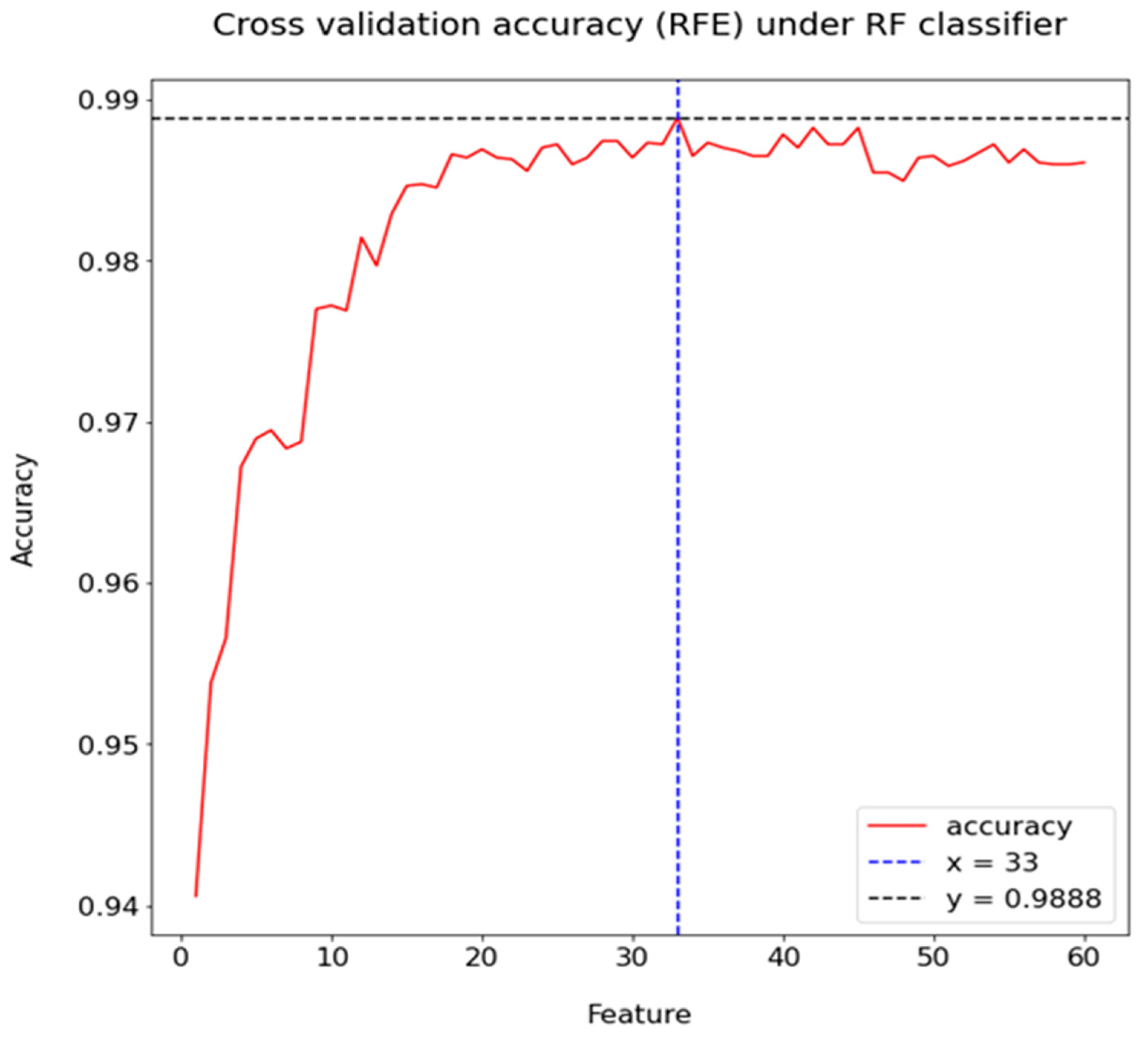
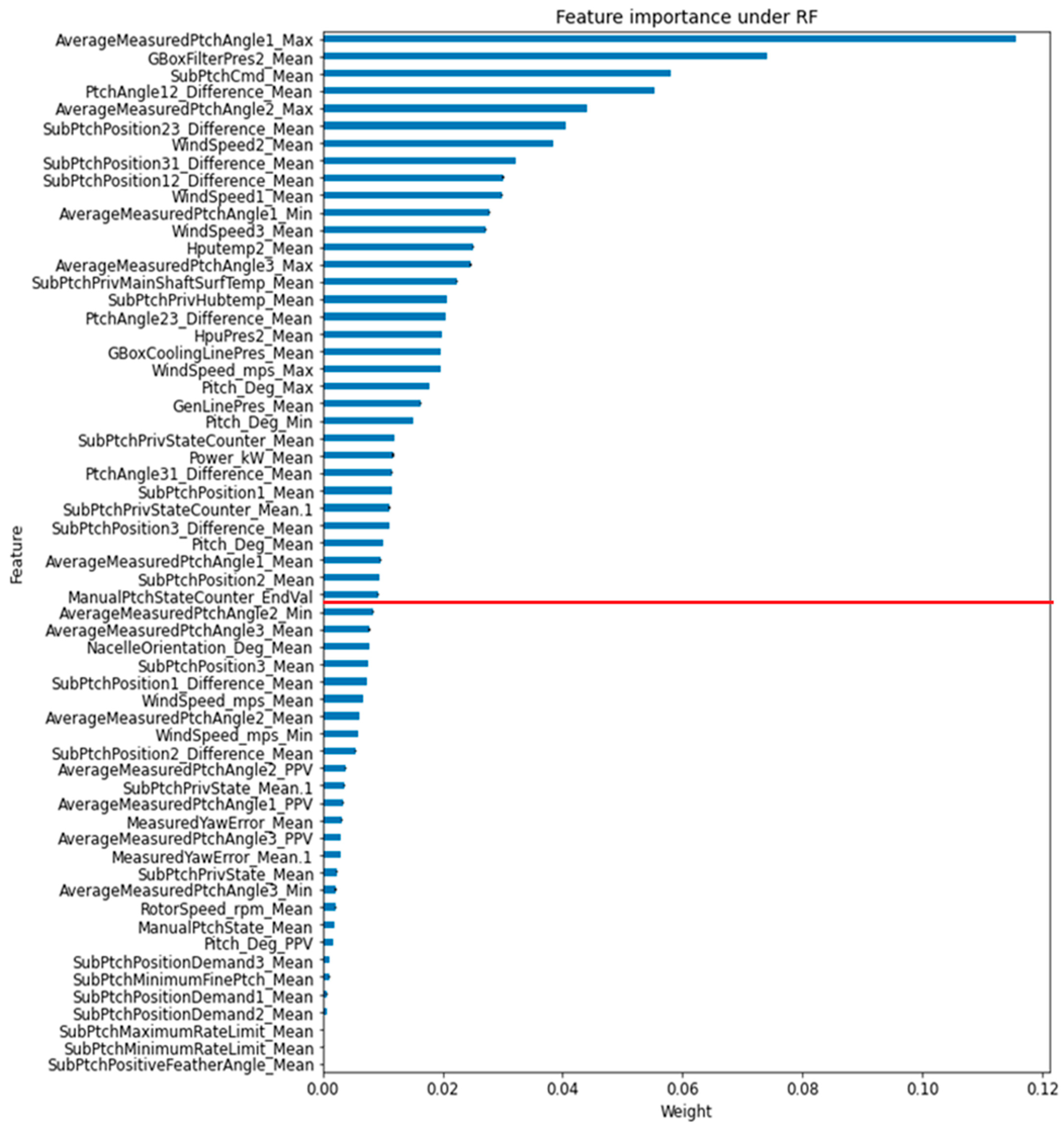
- A feature selection method, Recursive Feature Elimination (RFE) [34], is conducted along with an RF classifier for WT fault prediction. The weights of each feature are computed under the RF classifier, and the RFE application reserves the optimal number of features in order of their significance levels to maintain a balance between prediction accuracy and computational costs.
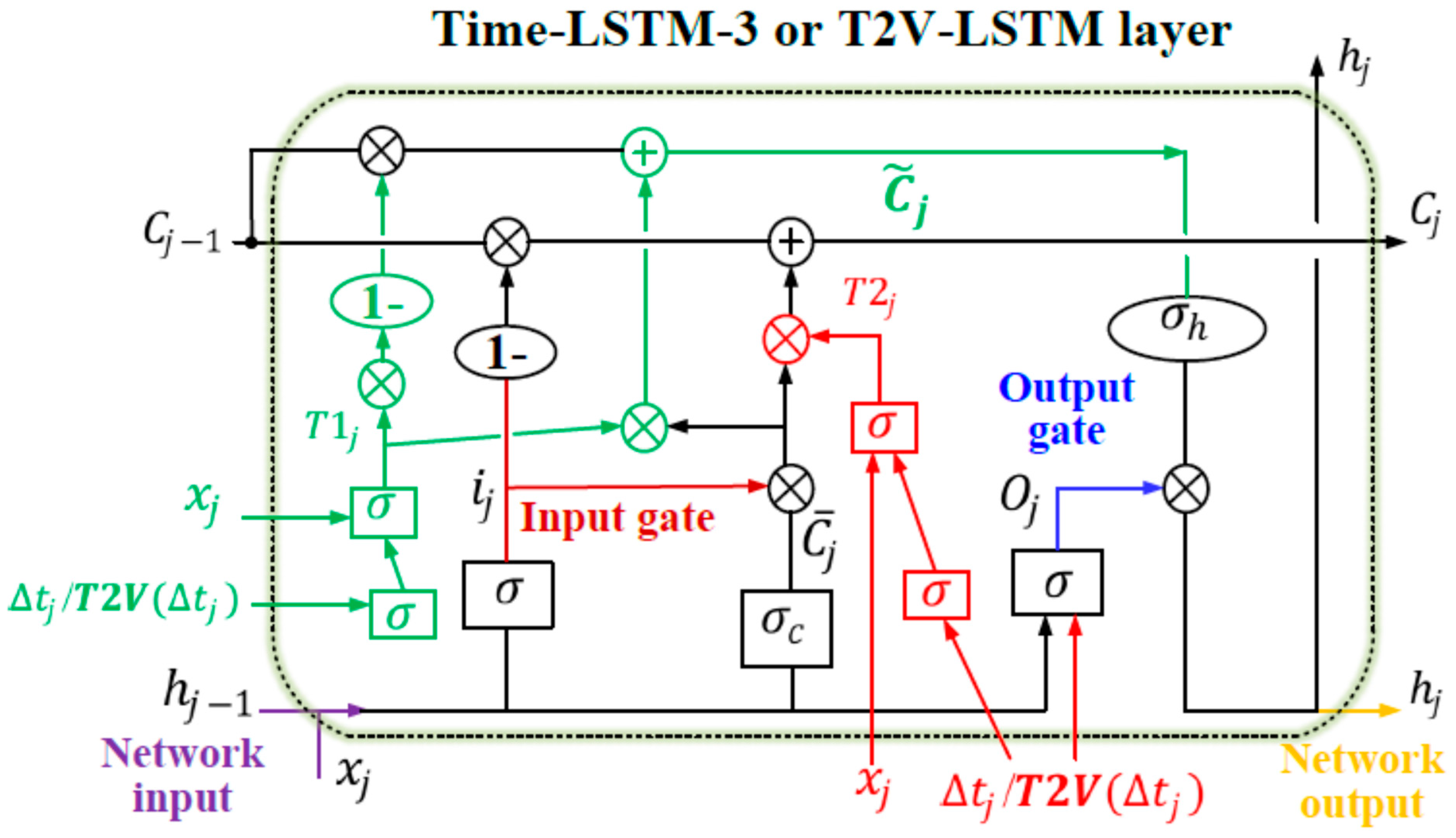
- By integrating Time2Vec into LSTM, this approach, T2V-LSTM, has been validated to outperform LSTM with a stationary Time2Vec activation function based on several synchronous datasets [33]. In this paper, the data points related to downtimes are removed to reserve only fault-free and fault data provided by the SCADA system for the purpose of fault and no-fault predictions. Thus, a non-stationary Time2Vec activation function is demanded to deal with the yielded asynchronous data.
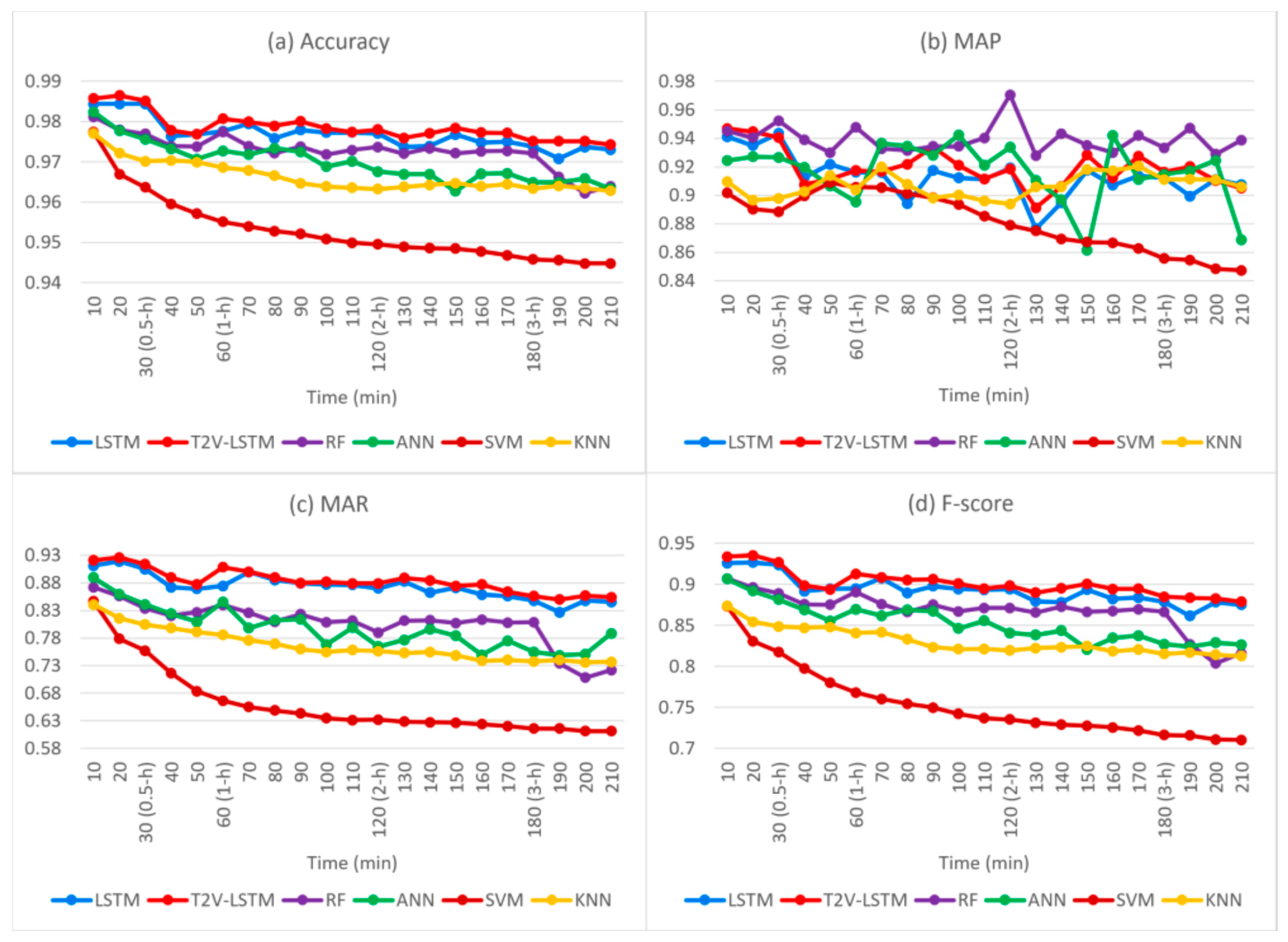
- A novel deep-learning neural network model, T2V-LSTM, with an optimal non-stationary activation function, is modelled to improve the model performance of LSTM, successfully detecting over 84.97% of faults in advance. The comparative studies between T2V-LSTM, LSTM, and other ML classifiers are investigated for overall and individual fault predictions based on performance metrics, including accuracy, recall scores, precision scores, and F-scores [16].
2. SCADA Data
2.1. Operational Data and Status Data
2.2. Feature Engineering
2.3. Predictive Fault Diagnosis
3. Methods
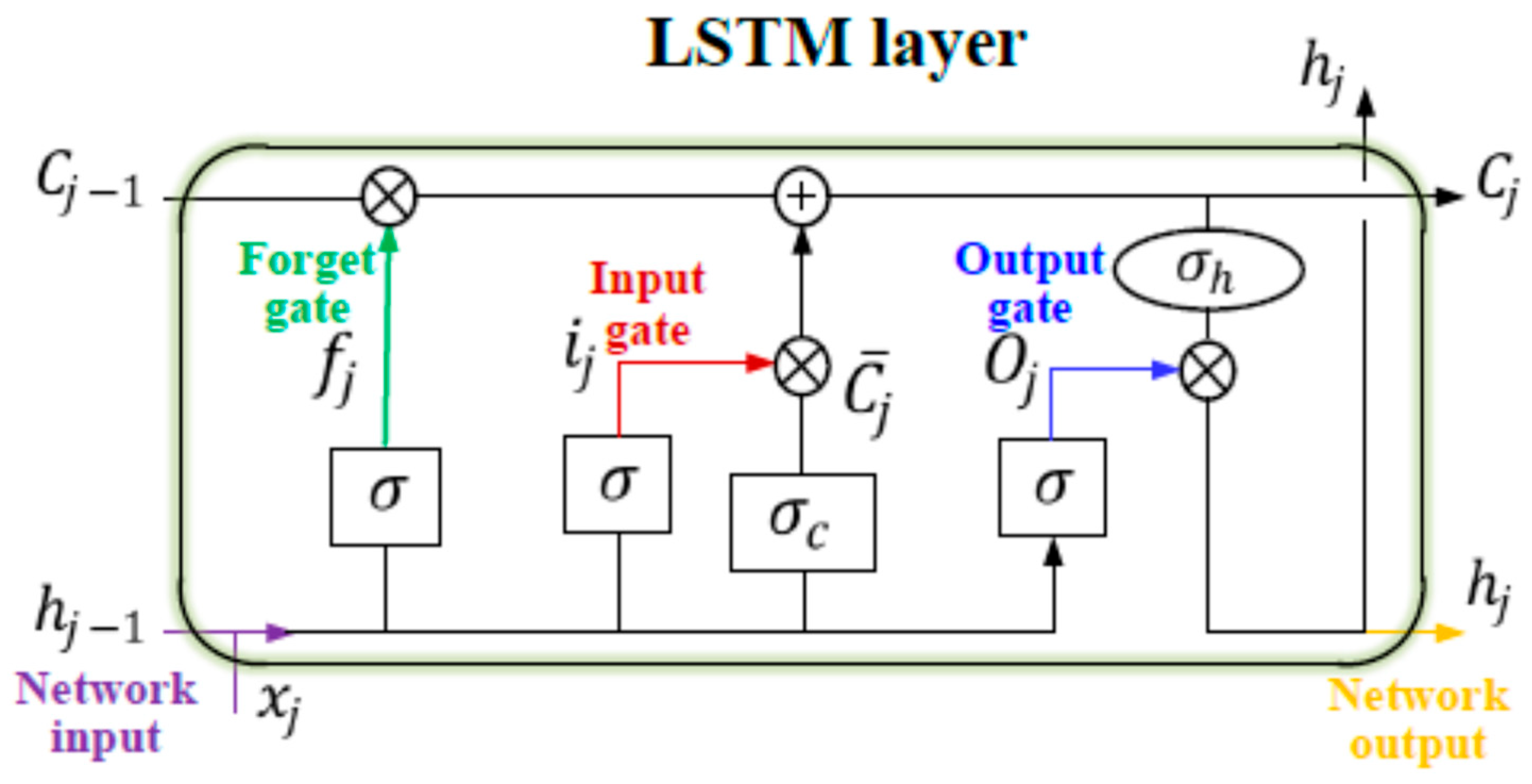
3.1. LSTM
3.2. Time-LSTM-1
3.3. Time-LSTM-3 and T2V-LSTM Models
3.4. Validations
3.5. Model Optimisation
4. Results
4.1. Overall Performance Metrics
4.2. Performance Metrics upon Individual Faults
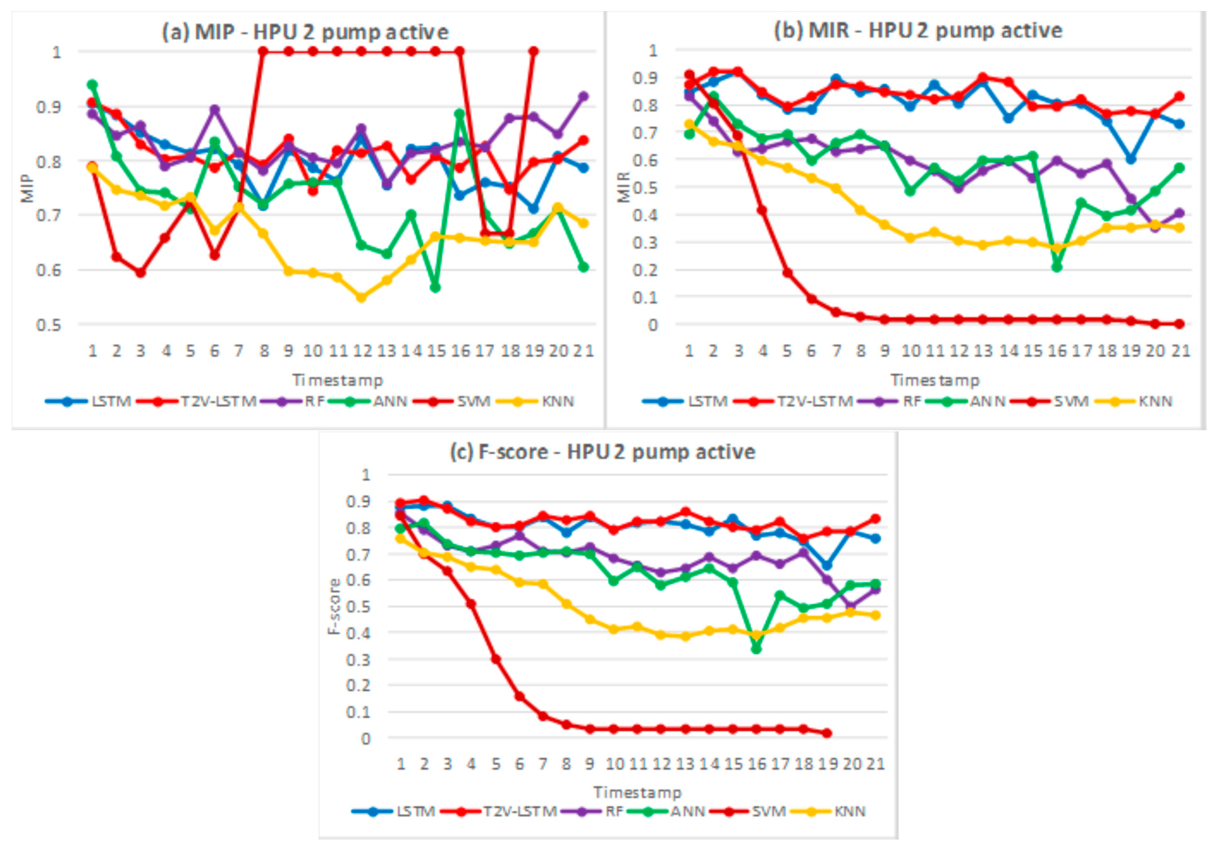
4.2.1. HPU 2 Pump Active
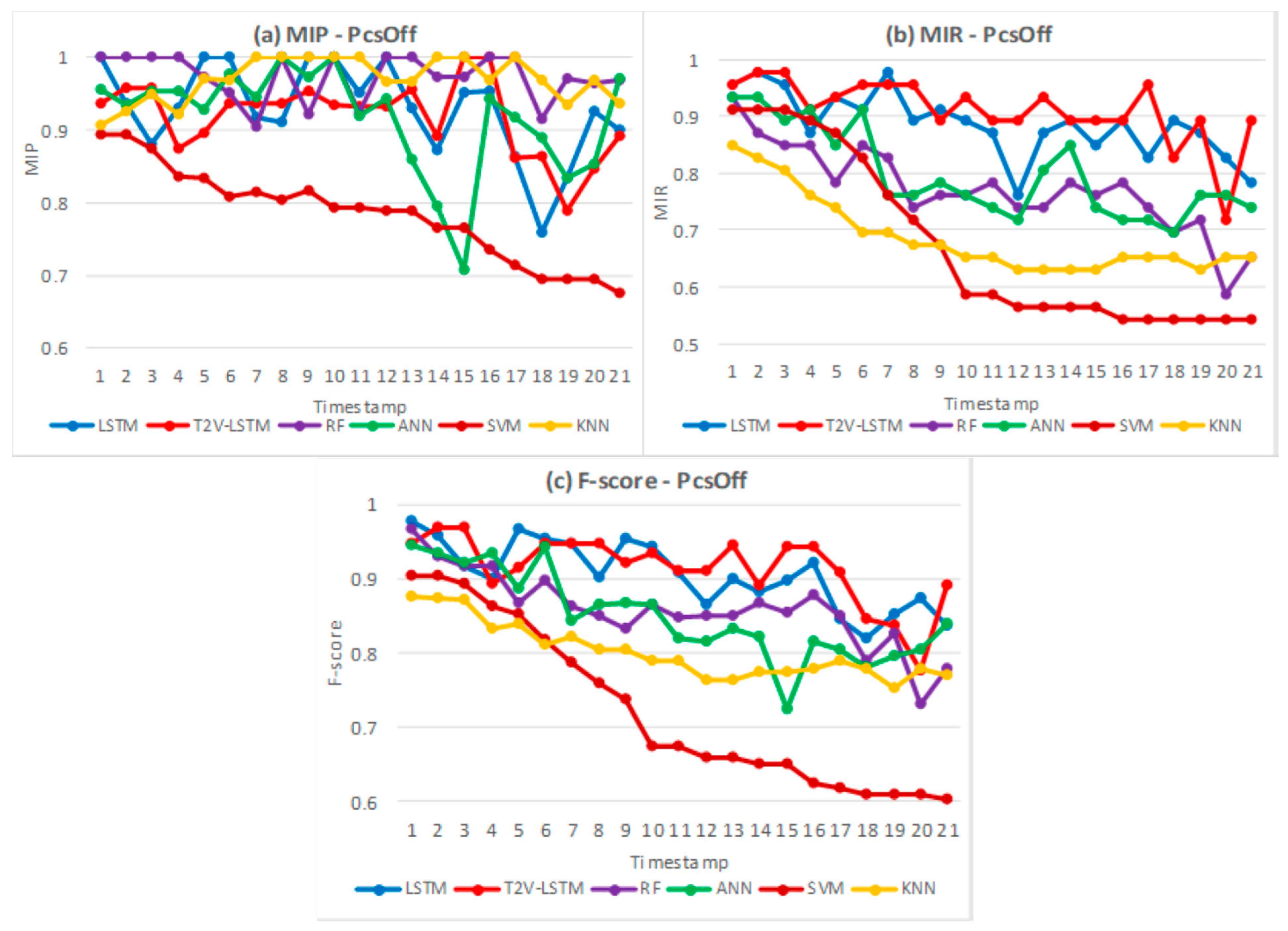
4.2.2. PcsOff
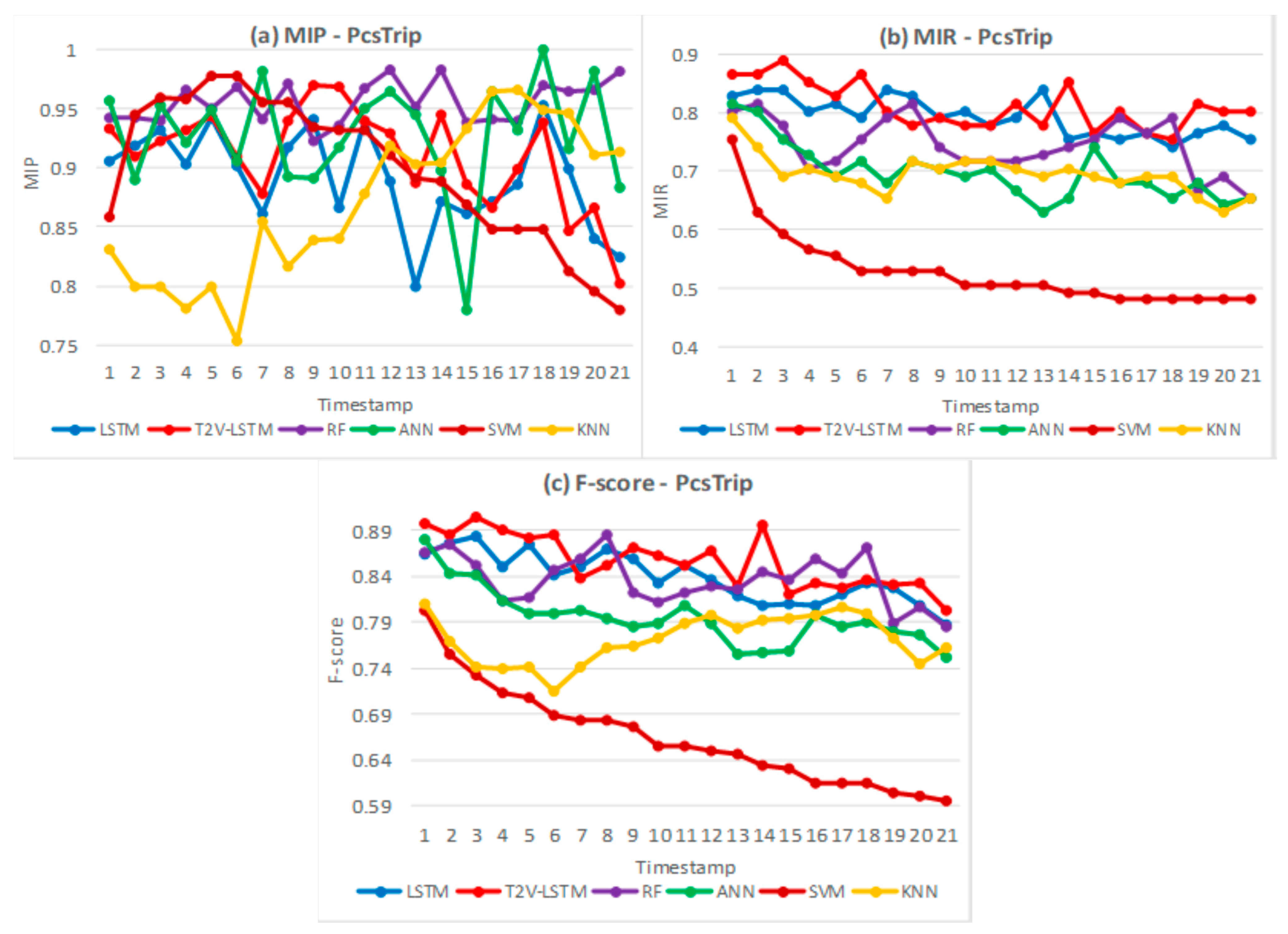
4.2.3. PcsTrip
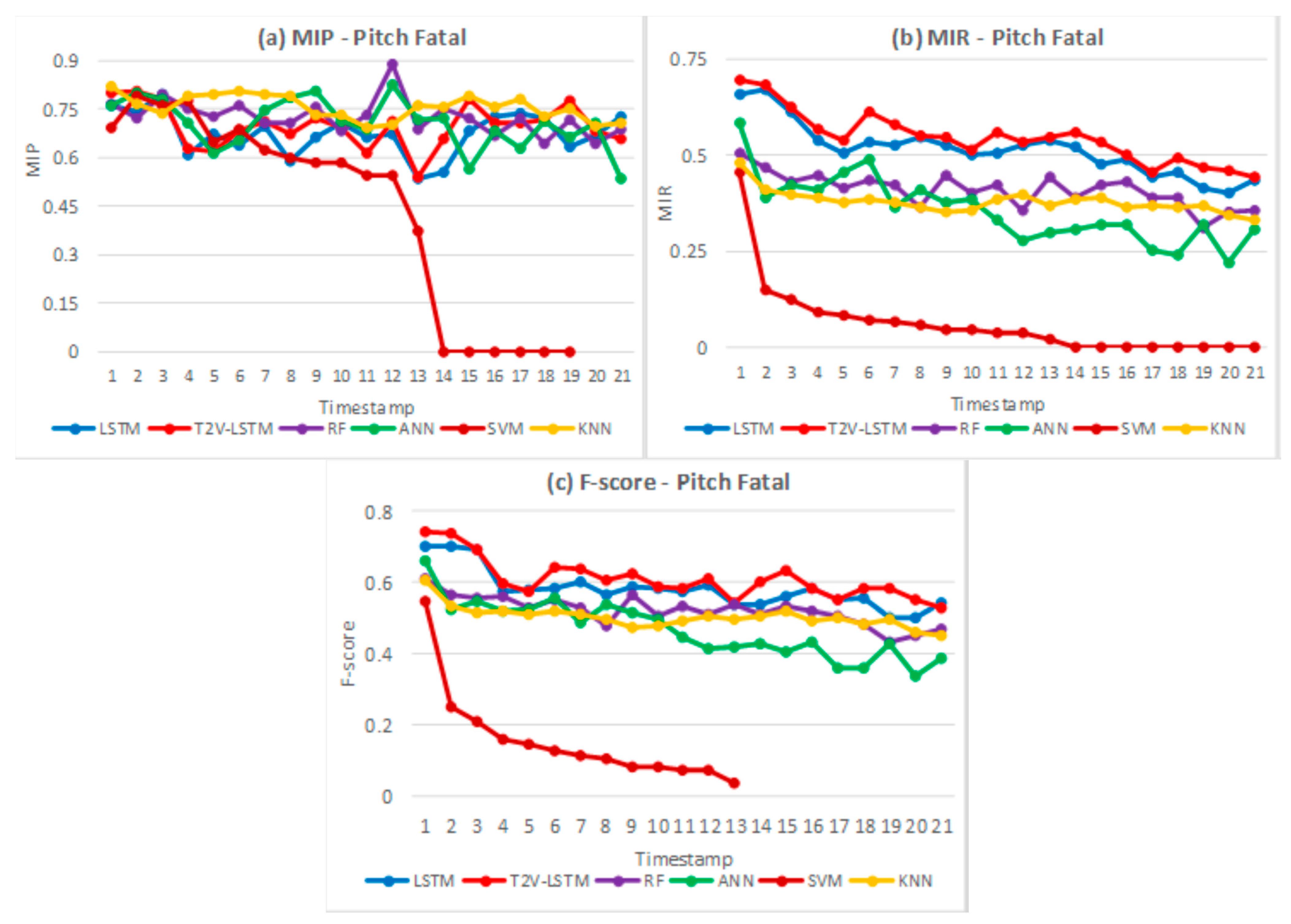
4.2.4. Pitch Fatal Faults
5. Discussion
5.1. Overall Performance Metrics
5.2. Individual Performance Metrics
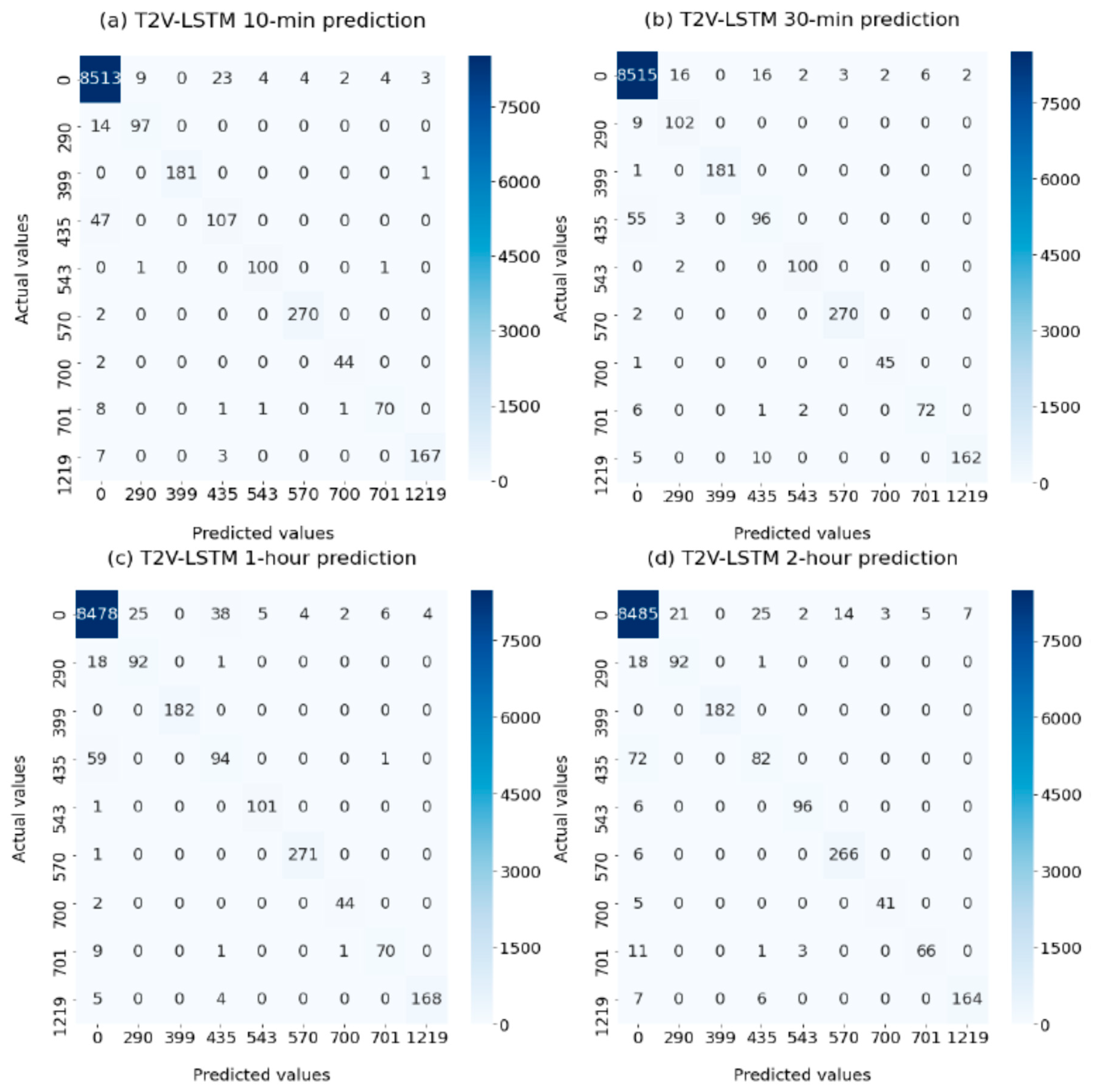
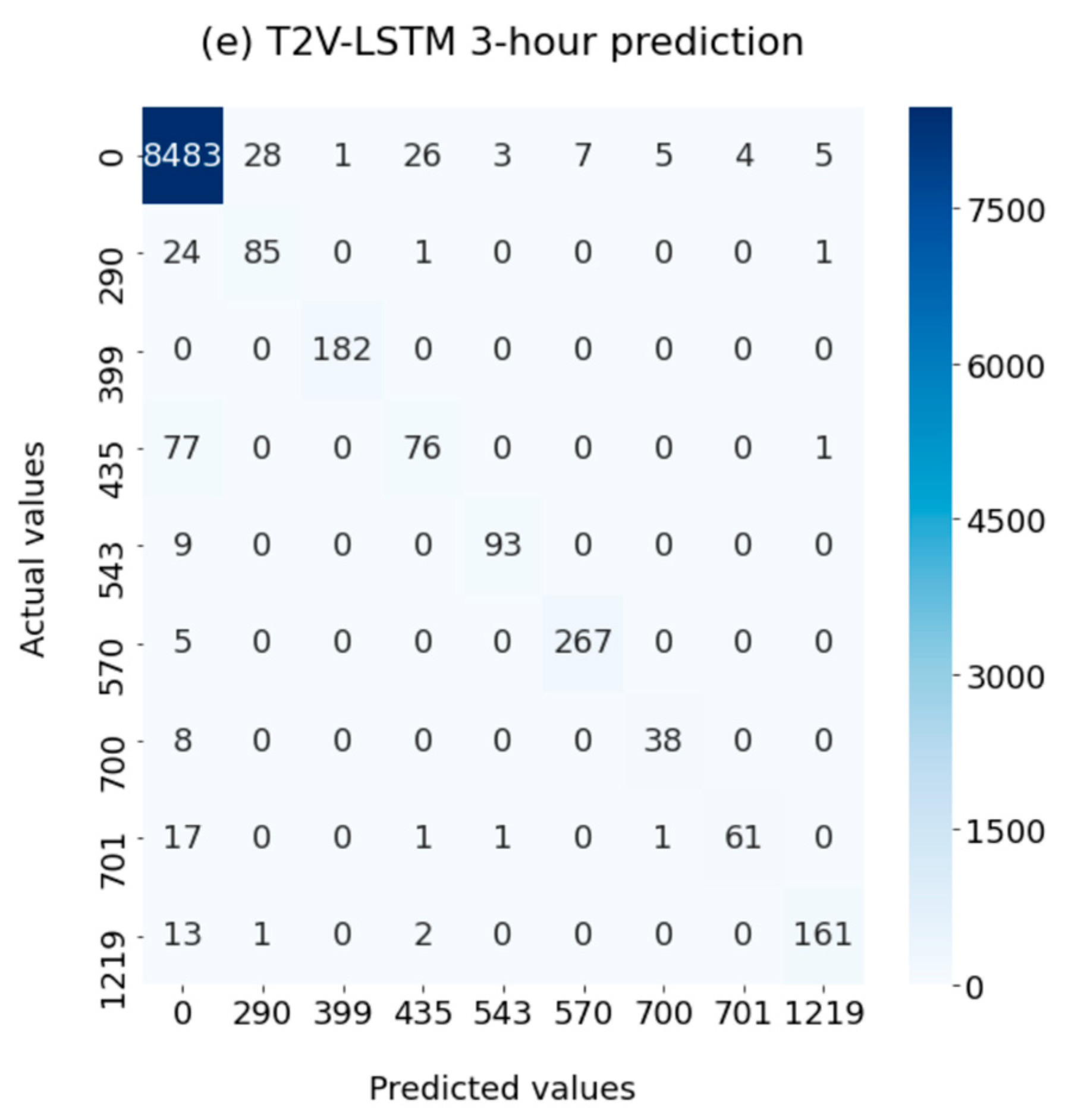
5.3. Confusion Matrix
6. Conclusions
- As there are eight specific faults and massive data imbalances studied in this research, T2V-LSTM can successfully predict all faults 160 min before their occurrence with an overall recall score (MAR) of over 87.5%. T2V-LSTM outperforms LSTM and other classifiers in terms of accuracy, recall scores (both MARs and MIRs), and F-scores in all test cases, but with a longer lagged time, the MAR abruptly falls to roughly 85%.
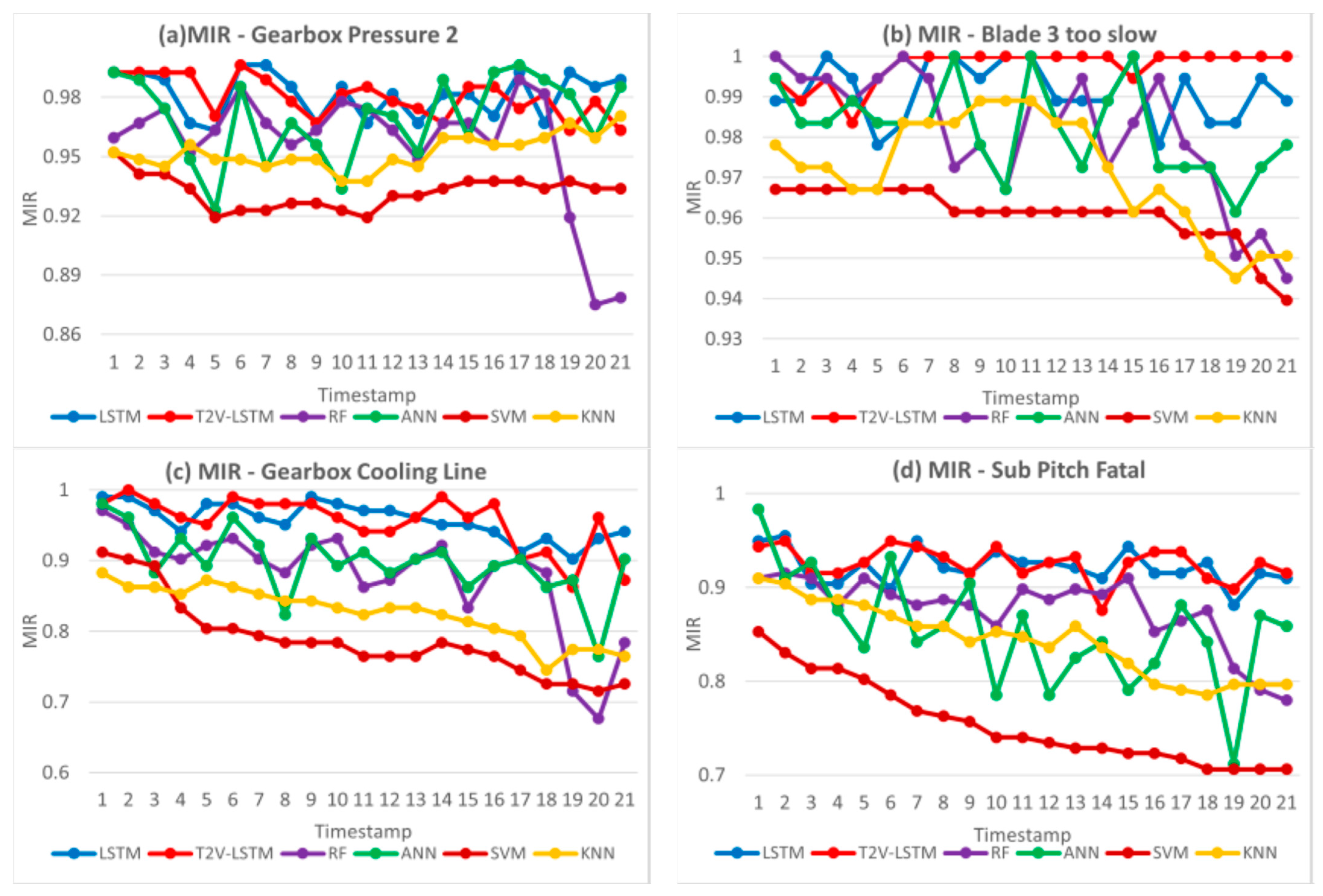
- T2V-LSTM has satisfactory predictions on (Demoted) gearbox pressure 2 faults, Blade 3 slow response, gearbox cooling faults, and sub-pitch fatal faults, due to its minimum MIP over 88.28% and minimum MIR over 86.27%, shown in Appendix A. Approximately 80% of the HPU 2 pump active faults are correctly predicted along with the relevant MIPs scoring roughly 80%. PcsOff faults exhibit excellent prediction results 160 min before the occurrence, with both recall and precision scores over 89%, but the significantly curtailed MIPs and MIRs take place over a longer prediction horizon. The F-scores on those faults are balanced due to their unbiased and promising precision and recall decisions.
- However, the balance between MIPs and MIRs is demolished under PcsTrip and pitch fatal faults due to their F-scores being brought down by poorer recall scores. PcsTrip and pitch fatal faults behold upper MIP ranges than MIR ranges and degraded predictions over time. PcsTrip faults are successfully predicted 30 min in advance due to their optimal MIR (88.88%), but the minimum MIR (75.30%) is obtained 3 h before occurrence. By comparison, MIRs on pitch fatal faults have an even more critical downtrend, reducing from 69.48% to 44.15% over time. Particularly, over half of pitch fatal faults are misdiagnosed >170 min before occurrence. The curtailments in MIRs on pitch fatal faults over 40 min ahead predominately contribute to the significant degradations of overall accuracy, MARs, and F-scores. Hence, the poorest predictions on pitch fatal faults bear a considerable burden for overall prediction accuracy.
- The confusion matrices visually study the balance between recall and precision scores by predicting the faults 10, 30, 60, 120, and 180 min in advance. Apart from PcsTrip and pitch fatal faults having more biases in FNs over FPs, the other faults can acquire the balanced F-scores due to their FNs roughly equalising FPs. For those faults with balanced F-scores, the resultant MIPs and MIRs mostly surpass 80%, except for the MIP (74.56%) and MIR (76.57%) from the 3 h ahead prediction on HPU 2 pump active faults. PcsTrip faults mainly have excellent MIPs over 90%, but the degradations on their MIRs are expected over time. Hence, the prediction curtailments provided by HPU 2 pump active faults and PcsTrip faults over a longer prediction horizon also contribute to the degradation of overall performance metrics.
- As T2V-LSTM fails to predict over 40% of pitch fatal faults 40 min prior to occurrence, future studies should critically focus on building a performance curve of pitch angle to improve the predictions on pitch fatal faults.
Author Contributions
Funding
Data Availability Statement
Acknowledgments
Conflicts of Interest
Appendix A

| Scores | Classifier (Four Other Individual Faults) | |||||||
|---|---|---|---|---|---|---|---|---|
| LSTM | T2V-LSTM | RF | ANN | SVM | KNN | ALL | ||
| MIP | MIN | 0.90654 | 0.8828829 | 0.90789 | 0.84444 | 0.8038 | 0.85106 | 0.8038 |
| MAX | 1 | 1 | 1 | 1 | 0.99435 | 0.99425 | 1 | |
| MIR | MIN | 0.88136 | 0.8627451 | 0.67647 | 0.71186 | 0.70621 | 0.7451 | 0.67647 |
| MAX | 1 | 1 | 1 | 1 | 0.96703 | 0.98901 | 1 | |
| F-score | MIN | 0.90698 | 0.9035533 | 0.77528 | 0.82353 | 0.75758 | 0.82162 | 0.75758 |
| MAX | 1 | 1 | 1 | 1 | 0.9805 | 0.97814 | 1 | |

References
- Singh, U.; Rizwan, M.; Malik, H. Wind Energy Scenario, Success and Initiatives Towards. Energies 2022, 15, 2291. [Google Scholar] [CrossRef]
- Sommer, B.; Pinson, P.; Messner, J.W.; Obst, D. Online Distributed Learning in Wind Power Forecasting. Int. J. Forecast. 2021, 37, 205–223. [Google Scholar] [CrossRef]
- Maldonado-Correa, J.; Solano, J.C.; Rojas-Moncayo, M. Wind Power Forecasting: A Systematic Literature Review. Wind Eng. 2021, 45, 413–426. [Google Scholar] [CrossRef]
- Kaldellis, J.K.; Apostolou, D.; Kapsali, M.; Kondili, E. Environmental and Social Footprint of Offshore Wind Energy Comparison with Onshore Counterpart. Renew. Energy 2016, 92, 543–556. [Google Scholar] [CrossRef]
- Al-Hinai, A.; Charabi, Y.; Kaboli, S.H.A. Offshore Wind Energy Resource Assessment across the Territory of Oman: A Spatial-Temporal Data Analysis. Sustainability 2021, 13, 2862. [Google Scholar] [CrossRef]
- Gao, Z.; Liu, X. An Overview on Fault Diagnosis, Prognosis and Resilient Control for Wind Turbine Systems. Processes 2021, 9, 300. [Google Scholar] [CrossRef]
- Zhang, S.; Robinson, E.; Basu, M. Hybrid Gaussian Process Regression and Fuzzy Inference System Based Approach for Condition Monitoring at the Rotor Side of a Doubly Fed Induction Generator. Renew. Energy 2022, 198, 936–946. [Google Scholar] [CrossRef]
- Leite, G.dN.P.; Araújo, A.M.; Rosas, P.A.C. Prognostic Techniques Applied to Maintenance of Wind Turbines: A Concise and Specific Review. Renew. Sustain. Energy Rev. 2018, 81, 1917–1925. [Google Scholar] [CrossRef]
- Sun, Y.; Kang, J.; Sun, L.; Jin, P.; Bai, X. Condition-Based Maintenance for the Offshore Wind Turbine Based on Long Short-Term Memory Network. Proc. Inst. Mech. Eng. Part O J. Risk Reliab. 2022, 236, 542–553. [Google Scholar] [CrossRef]
- Koukoura, S.; Peeters, C.; Helsen, J.; Carroll, J. Investigating Parallel Multi-Step Vibration Processing Pipelines for Planetary Stage Fault Detection in Wind Turbine Drivetrains Investigating Parallel Multi-Step Vibration Processing Pipelines for Planetary Stage Fault Detection in Wind Turbine Drivetrains. J. Phys. Conf. Ser. 2020, 1618, 022054. [Google Scholar] [CrossRef]
- Raposo, H.; Farinha, J.T.; Fonseca, I.; Galar, D. Predicting Condition Based on Oil Analysis—A Case Study. Tribol. Int. 2019, 135, 65–74. [Google Scholar] [CrossRef]
- Zappalá, D.; Sarma, N.; Djurović, S.; Crabtree, C.J.; Mohammad, A.; Tavner, P.J. Electrical & Mechanical Diagnostic Indicators of Wind Turbine Induction Generator Rotor Faults. Renew. Energy 2019, 131, 14–24. [Google Scholar] [CrossRef]
- Yang, W.; Peng, Z.; Wei, K.; Tian, W. Structural Health Monitoring of Composite Wind Turbine Blades: Challenges, Issues and Potential Solutions. IET Renew. Power Gener. 2017, 11, 411–416. [Google Scholar] [CrossRef]
- Yang, W.; Tavner, P.J.; Crabtree, C.J.; Feng, Y.; Qiu, Y. Wind Turbine Condition Monitoring: Technical and Commercial Challenges. Wind Energy 2014, 17, 673–693. [Google Scholar] [CrossRef]
- Tautz-Weinert, J.; Watson, S.J. Using SCADA Data for Wind Turbine Condition Monitoring—A Review. IET Renew. Power Gener. 2017, 11, 382–394. [Google Scholar] [CrossRef]
- Stetco, A.; Dinmohammadi, F.; Zhao, X.; Robu, V.; Flynn, D.; Barnes, M.; Keane, J.; Nenadic, G. Machine Learning Methods for Wind Turbine Condition Monitoring: A Review. Renew. Energy 2019, 133, 620–635. [Google Scholar] [CrossRef]
- Sahnoun, M.; Baudry, D.; Mustafee, N.; Louis, A.; Smart, P.A.; Godsiff, P.; Mazari, B. Modelling and Simulation of Operation and Maintenance Strategy for Offshore Wind Farms Based on Multi-Agent System. J. Intell. Manuf. 2019, 30, 2981–2997. [Google Scholar] [CrossRef]
- Lu, L.; He, Y.; Wang, T.; Shi, T.; Li, B. Self-Powered Wireless Sensor for Fault Diagnosis of Wind Turbine Planetary Gearbox. IEEE Access 2019, 7, 87382–87395. [Google Scholar] [CrossRef]
- Leahy, K.; Hu, R.L.; Konstantakopoulos, I.C.; Spanos, C.J.; Agogino, A.M.; Sullivan, D.T.J.O. Diagnosing and Predicting Wind Turbine Faults from SCADA Data Using Support Vector Machines. Int. J. Progn. Health Manag. 2018, 9, 1–11. [Google Scholar]
- Naik, S.; Koley, E. Fault Detection and Classification Scheme Using KNN for AC/HVDC Transmission Lines. In Proceedings of the 2019 International Conference on Communication and Electronics Systems (ICCES), Coimbatore, India, 17–19 July 2019; pp. 1131–1135. [Google Scholar] [CrossRef]
- Marti-Puig, P.; Blanco-M, A.; Cárdenas, J.J.; Cusidó, J.; Solé-Casals, J. Feature selection algorithms for wind turbine failure prediction. Energies 2019, 12, 453. [Google Scholar] [CrossRef]
- Ibrahim, R.K.; Tautz-Weinert, J.; Watson, S.J. Neural Networks for Wind Turbine Fault Detection via Current Signature Analysis; Wind Europe: Hamburg, Germany, 2016. [Google Scholar]
- Kandukuri, S.T.; Senanyaka, J.S.L.; Huynh, V.K.; Robbersmyr, K.G. A Two-Stage Fault Detection and Classification Scheme for Electrical Pitch Drives in Offshore Wind Farms Using Support Vector Machine. IEEE Trans. Ind. Appl. 2019, 55, 5109–5118. [Google Scholar] [CrossRef]
- Malik, H.; Mishra, S. Artificial Neural Network and Empirical Mode Decomposition Based Imbalance Fault Diagnosis of Wind Turbine Using TurbSim, FAST and Simulink. IET Renew. Power Gener. 2017, 11, 889–902. [Google Scholar] [CrossRef]
- Yang, X.; Zhang, Y.; Lv, W.; Wang, D. Image Recognition of Wind Turbine Blade Damage Based on a Deep Learning Model with Transfer Learning and an Ensemble Learning Classifier. Renew. Energy 2021, 163, 386–397. [Google Scholar] [CrossRef]
- Zhang, D.; Qian, L.; Mao, B.; Huang, C.; Huang, B.; Si, Y. A Data-Driven Design for Fault Detection of Wind Turbines Using Random Forests and XGboost. IEEE Access 2018, 6, 21020–21031. [Google Scholar] [CrossRef]
- Helbing, G.; Ritter, M. Deep Learning for Fault Detection in Wind Turbines. Renew. Sustain. Energy Rev. 2018, 98, 189–198. [Google Scholar] [CrossRef]
- Chung, J.; Gulcehre, C.; Cho, K.; Bengio, Y. Empirical Evaluation of Gated Recurrent Neural Networks on Sequence Modeling. arXiv 2014, arXiv:1412.3555. [Google Scholar]
- Hochreiter, S.; Schmidhuber, J. Long Short-Term Memory. Neural Comput. 1997, 9, 1735–1780. [Google Scholar] [CrossRef]
- Chen, H.; Liu, H.; Chu, X.; Liu, Q.; Xue, D. Anomaly Detection and Critical SCADA Parameters Identi Fi Cation for Wind Turbines Based on LSTM-AE Neural Network. Renew. Energy 2021, 172, 829–840. [Google Scholar] [CrossRef]
- Lei, J.; Liu, C.; Jiang, D. Fault Diagnosis of Wind Turbine Based on Long Short-Term Memory Networks. Renew. Energy 2019, 133, 422–432. [Google Scholar] [CrossRef]
- Yu, L.; Qu, J.; Gao, F.; Tian, Y. A Novel Hierarchical Algorithm for Bearing Fault Diagnosis Based on Stacked LSTM. Shock Vib. 2019, 2019, 2756284. [Google Scholar] [CrossRef]
- Kazemi, S.M.; Goel, R.; Eghbali, S.; Ramanan, J.; Sahota, J.; Thakur, S.; Wu, S.; Smyth, C.; Poupart, P.; Brubaker, M. Time2Vec: Learning a Vector Representation of Time. arXiv 2019, arXiv:1907.05321. [Google Scholar]
- Granitto, P.M.; Furlanello, C.; Biasioli, F.; Gasperi, F. Recursive Feature Elimination with Random Forest for PTR-MS Analysis of Agroindustrial Products. Chemom. Intell. Lab. Syst. 2006, 83, 83–90. [Google Scholar] [CrossRef]
- ORE Catapult. Levenmouth 7MW Demonstration Offshore Wind Turbine Specification Sheet. 2016, Volume 44, pp. 7–8. Available online: https://ore.catapult.org.uk/app/uploads/2018/01/Levenmouth-7MW-demonstration-offshore-wind-turbine.pdf (accessed on 10 September 2023).
- Serret, J.; Rodriguez, C.; Tezdogan, T.; Stratford, T.; Thies, P. Code Comparison of a NREL-Fast Model of the Levenmouth Wind Turbine with the GH Bladed Commissioning Results. In Proceedings of the ASME 2018 37th International Conference on Ocean, Offshore and Arctic Engineering, Madrid, Spain, 17–22 June 2018; Volume 10. [Google Scholar] [CrossRef]
- Kusiak, A.; Li, W. The Prediction and Diagnosis of Wind Turbine Faults. Renew. Energy 2011, 36, 16–23. [Google Scholar] [CrossRef]
- Kusiak, A.; Verma, A. A Data-Driven Approach for Monitoring Blade Pitch Faults in Wind Turbines. IEEE Trans. Sustain. Energy 2011, 2, 87–96. [Google Scholar] [CrossRef]
- Zhu, Y.; Li, H.; Liao, Y.; Wang, B.; Guan, Z.; Liu, H.; Cai, D.; Science, C. What to Do Next: Modeling User Behaviors by Time-LSTM. IJCAI 2017, 17, 3602–3608. [Google Scholar] [CrossRef]
- Greff, K.; Srivastava, R.K.; Koutn, J.; Steunebrink, B.R. LSTM: A Search Space Odyssey. IEEE Trans. Neural Netw. Learn. Syst. 2016, 28, 2222–2232. [Google Scholar] [CrossRef]
- Suzuki, K. Artificial Neural Networks—Methodological Advances and Biomedical Applications; Intech: Rijeka, Croatia, 2011; Available online: https://www.intechopen.com/books/citations/artificial-neural-networks-methodological-advances-and-biomedical-applications (accessed on 10 September 2023).
- Brownlee, J. How to Grid Search Hyperparameters for Deep Learning Models in Python with Keras. 2016. Available online: https://machinelearningmastery.com/grid-search-hyperparameters-deeplearning-models-python-keras (accessed on 10 September 2023).
- Sharma, S. Activation functions in neural networks. Towards Data Sci. 2020, 4, 310–316. [Google Scholar] [CrossRef]


| StartTime | WindSpeed _mps_Min | WindSpeed _mps_Max | WindSpeed _mps_Mean | WindSpeed _mps_Stdev | WindSpeed _mps_EndVal |
|---|---|---|---|---|---|
| 21/05/2018 22:00:00 | 3.577394 | 10.11077 | 6.8690084 | 1.3447459 | 5.802108 |
| 21/05/2018 22:10:00 | 3.062414 | 10.03982 | 6.7177955 | 1.108204 | 6.073331 |
| 21/05/2018 22:20:00 | 4.69204 | 9.636992 | 7.1981784 | 1.0209401 | 8.475427 |
| TimeOn | TimeOff | Event Code | Event Description |
|---|---|---|---|
| 21/05/2018 19:38:33 | 21/05/2018 19:38:39 | 286 | (Demoted) Yaw Hydraulic Pressure Diff Too Large |
| 21/05/2018 20:26:02 | 21/05/2018 20:26:10 | 543 | Gearbox Cooling Line Pressure Too Low |
| 21/05/2018 20:26:12 | 21/05/2018 20:29:20 | 543 | Gearbox Cooling Line Pressure Too Low |
| Event Code | Frequency | Description |
|---|---|---|
| 0 | 42,598 | Fault-free |
| 290 | 565 | HPU 2 pump active for too long |
| 399 | 998 | Blade 3 too slow to respond |
| 435 | 826 | Pitch system fatal error |
| 543 | 522 | Gearbox cooling line pressure too low |
| 570 | 1436 | (Demoted) gearbox filter manifold pressure 2 shutdown |
| 700 | 701 | PcsOff *1 |
| 701 | 417 | PcsTrip *2 |
| 1219 | 816 | Sub-pitch priv fatal error has occurred more than 3 times |
| Hyper Parameter | Grid | Optimisation |
|---|---|---|
| Batch size | 10, 20, 25, 40, 50, 60, 80, 100 | 25 |
| Number of Epochs | 10, 20, 25, 40, 50, 60, 80, 100 | 100 |
| Activation function () | Elu, Relu, Sigmoid, Sine (only Time2Vec), Softmax, Softplus, Softsign, Tanh | Tanh |
| Activation function () | Elu, Relu, Sigmoid, Softmax, Softplus, Softsign, Tanh | Tanh |
| Activation function () | Elu, Relu, Sigmoid, Softmax, Softplus, Softsign, Tanh | Softmax |
| Scores | Classifier (Overall Fault) | |||||||
|---|---|---|---|---|---|---|---|---|
| LSTM | T2V-LSTM | RF | ANN | SVM | KNN | ALL | ||
| Accuracy | MIN | 0.97079 | 0.9742954 | 0.96222 | 0.96273 | 0.94477 | 0.96284 | 0.94477 |
| MAX | 0.98441 | 0.9864767 | 0.97791 | 0.9777 | 0.96697 | 0.97213 | 0.98648 | |
| MAP | MIN | 0.87643 | 0.8912656 | 0.92785 | 0.86133 | 0.84729 | 0.89391 | 0.84729 |
| MAX | 0.94347 | 0.9469835 | 0.97052 | 0.9422 | 0.90898 | 0.92044 | 0.97052 | |
| MAR | MIN | 0.82667 | 0.8497778 | 0.70844 | 0.74844 | 0.61156 | 0.736 | 0.61156 |
| MAX | 0.91911 | 0.9262222 | 0.872 | 0.88978 | 0.84711 | 0.84089 | 0.92622 | |
| F-score | MIN | 0.86151 | 0.8788294 | 0.80383 | 0.82085 | 0.71038 | 0.81275 | 0.71038 |
| MAX | 0.92694 | 0.935368 | 0.90707 | 0.9067 | 0.87351 | 0.8739 | 0.93537 | |
| Execution time (s) | MIN | 299.0876 | 309.44707 | 281.5733 | 232.2455 | 174.6638 | 148.6676 | 148.6676 |
| MAX | 337.6192 | 346.63702 | 322.1635 | 281.5004 | 326.7903 | 186.6617 | 346.63702 | |
| Scores | Classifier (HPU 2 Pump Active) | |||||||
|---|---|---|---|---|---|---|---|---|
| LSTM | T2V-LSTM | RF | ANN | SVM | KNN | ALL | ||
| MIP | MIN | 0.71277 | 0.744 | 0.7561 | 0.56667 | 0.59375 | 0.54839 | 0.54839 |
| MAX | 0.90385 | 0.9065421 | 0.91837 | 0.93902 | 1 | 0.78641 | 1 | |
| MIR | MIN | 0.6036 | 0.7657658 | 0.35135 | 0.20721 | 0 | 0.27928 | 0 |
| MAX | 0.91892 | 0.9189189 | 0.82883 | 0.82883 | 0.90991 | 0.72973 | 0.91892 | |
| F-score | MIN | 0.65366 | 0.7555556 | 0.49682 | 0.33577 | 0.01786 | 0.38554 | 0.01786 |
| MAX | 0.88312 | 0.9026549 | 0.85581 | 0.81778 | 0.84519 | 0.75701 | 0.90265 | |
| Scores | Classifier (PcsOff) | |||||||
|---|---|---|---|---|---|---|---|---|
| LSTM | T2V-LSTM | RF | ANN | SVM | KNN | ALL | ||
| MIP | MIN | 0.75926 | 0.7884615 | 0.90476 | 0.70833 | 0.67568 | 0.90698 | 0.67568 |
| MAX | 1 | 1 | 1 | 1 | 0.89362 | 1 | 1 | |
| MIR | MIN | 0.76087 | 0.7173913 | 0.58696 | 0.69565 | 0.54348 | 0.63043 | 0.54348 |
| MAX | 0.97826 | 0.9782609 | 0.93478 | 0.93478 | 0.91304 | 0.84783 | 0.97826 | |
| F-score | MIN | 0.82 | 0.7764706 | 0.72973 | 0.7234 | 0.60241 | 0.75325 | 0.60241 |
| MAX | 0.97778 | 0.9677419 | 0.96629 | 0.94505 | 0.90323 | 0.8764 | 0.97778 | |
| Scores | Classifier (PcsTrip) | |||||||
|---|---|---|---|---|---|---|---|---|
| LSTM | T2V-LSTM | RF | ANN | SVM | KNN | ALL | ||
| MIP | MIN | 0.8 | 0.8024691 | 0.92308 | 0.77922 | 0.78 | 0.75342 | 0.75342 |
| MAX | 0.95238 | 0.969697 | 0.98361 | 1 | 0.97826 | 0.96552 | 1 | |
| MIR | MIN | 0.74074 | 0.7530864 | 0.65432 | 0.62963 | 0.48148 | 0.62963 | 0.48148 |
| MAX | 0.83951 | 0.8888889 | 0.81481 | 0.81481 | 0.75309 | 0.79012 | 0.88889 | |
| F-score | MIN | 0.7871 | 0.8024691 | 0.78519 | 0.75177 | 0.59542 | 0.71429 | 0.59542 |
| MAX | 0.88312 | 0.9056604 | 0.88591 | 0.88 | 0.80263 | 0.81013 | 0.90566 | |
| Scores | Classifier (Pitch Fatal Faults) | |||||||
|---|---|---|---|---|---|---|---|---|
| LSTM | T2V-LSTM | RF | ANN | SVM | KNN | ALL | ||
| MIP | MIN | 0.53548 | 0.5419355 | 0.64286 | 0.53409 | 0 | 0.69412 | 0 |
| MAX | 0.79661 | 0.8076923 | 0.8871 | 0.82692 | 0.7931 | 0.82222 | 0.8871 | |
| MIR | MIN | 0.4026 | 0.4415584 | 0.31169 | 0.22078 | 0 | 0.33117 | 0 |
| MAX | 0.66883 | 0.6948052 | 0.50649 | 0.58442 | 0.45455 | 0.48052 | 0.69481 | |
| F-score | MIN | 0.50196 | 0.5291829 | 0.43439 | 0.33663 | 0.03704 | 0.45133 | 0.03704 |
| MAX | 0.70383 | 0.7430556 | 0.60938 | 0.66176 | 0.54902 | 0.60656 | 0.74306 | |
Disclaimer/Publisher’s Note: The statements, opinions and data contained in all publications are solely those of the individual author(s) and contributor(s) and not of MDPI and/or the editor(s). MDPI and/or the editor(s) disclaim responsibility for any injury to people or property resulting from any ideas, methods, instructions or products referred to in the content. |
© 2023 by the authors. Licensee MDPI, Basel, Switzerland. This article is an open access article distributed under the terms and conditions of the Creative Commons Attribution (CC BY) license (https://creativecommons.org/licenses/by/4.0/).
Share and Cite
Zhang, S.; Robinson, E.; Basu, M. Wind Turbine Predictive Fault Diagnostics Based on a Novel Long Short-Term Memory Model. Algorithms 2023, 16, 546. https://doi.org/10.3390/a16120546
Zhang S, Robinson E, Basu M. Wind Turbine Predictive Fault Diagnostics Based on a Novel Long Short-Term Memory Model. Algorithms. 2023; 16(12):546. https://doi.org/10.3390/a16120546
Chicago/Turabian StyleZhang, Shuo, Emma Robinson, and Malabika Basu. 2023. "Wind Turbine Predictive Fault Diagnostics Based on a Novel Long Short-Term Memory Model" Algorithms 16, no. 12: 546. https://doi.org/10.3390/a16120546
APA StyleZhang, S., Robinson, E., & Basu, M. (2023). Wind Turbine Predictive Fault Diagnostics Based on a Novel Long Short-Term Memory Model. Algorithms, 16(12), 546. https://doi.org/10.3390/a16120546