Article

Comparing Activation Functions in Machine Learning for Finite Element Simulations in Thermomechanical Forming

Laboratoire Génie de Production, Institut National Polytechnique/Ecole Nationale d’Ingénieurs de Tarbes, Université de Toulouse, 47 Av d’Azereix, F-65016 Tarbes, France
Algorithms 2023, 16(12), 537; https://doi.org/10.3390/a16120537
Submission received: 27 October 2023 / Revised: 21 November 2023 / Accepted: 24 November 2023 / Published: 25 November 2023
(This article belongs to the Special Issue Artificial Intelligence in Modeling and Simulation)

Abstract

:
Finite element (FE) simulations have been effective in simulating thermomechanical forming processes, yet challenges arise when applying them to new materials due to nonlinear behaviors. To address this, machine learning techniques and artificial neural networks play an increasingly vital role in developing complex models. This paper presents an innovative approach to parameter identification in flow laws, utilizing an artificial neural network that learns directly from test data and automatically generates a Fortran subroutine for the Abaqus standard or explicit FE codes. We investigate the impact of activation functions on prediction and computational efficiency by comparing Sigmoid, Tanh, ReLU, Swish, Softplus, and the less common Exponential function. Despite its infrequent use, the Exponential function demonstrates noteworthy performance and reduced computation times. Model validation involves comparing predictive capabilities with experimental data from compression tests, and numerical simulations confirm the numerical implementation in the Abaqus explicit FE code.

1. Introduction

In industry and research, numerical simulations are commonly employed to predict the behavior of structures under severe thermomechanical conditions, such as high-temperature forming of metallic materials. These simulations rely on finite element (FE) codes, like Abaqus [1], or academic codes. The accuracy of these simulations is heavily influenced by constitutive equations and the identification of their parameters through experimental tests. These tests, conducted under conditions similar to the actual service loading, involve quasi-static or dynamic tensile/compression tests, thermomechanical simulators (e.g., Gleeble [2,3,4,5]), or impact tests using gas guns or Hopkinson bars [6]. The choice and formulation of behavior laws and the accurate identification of coefficients from experiments are crucial for obtaining reliable simulation results.

1.1. Constitutive Behavior and Material Flow Law

Thermomechanical behavior laws used in numerical integration algorithms such as the radial-return method [7] involve nonlinear flow law functions due to the complex nature of materials and associated phenomena like work hardening, dislocation movement, structural hardening, and phase transformations. The applicability of these flow laws is confined to specific ranges of deformations, strain rates, and temperatures. In the context of simulating forming processes, these behavior laws dictate how the material’s flow stress σ depends on three key input variables: strain ε , strain rate ε . , and temperature T. The general form of the flow law is expressed through a mathematical equation:
σ = σ ε , ε . , T .
The historical development of behavior laws for simulating hot forming processes, beginning in the 1950s, involved the use of power laws to describe strain/stress relationships, later adapted to incorporate temperature effects. In the 1970s, thermomechanical models evolved to include time dependence, linking flow laws to strain rate and time. Notable models like the Johnson–Cook [8], Zerilli–Armstrong [9], and Arrhenius [10] flow laws emerged and are commonly used in forming process simulations. The selection of a flow law for simulating material behavior in finite element analysis is crucial, and it should be based on experimental tests conducted under conditions resembling real-world applications. Researchers face a challenge in choosing the appropriate flow law after characterizing experimental behavior. This decision is influenced by the availability of flow laws within the finite element analysis software being used. For instance, users of Abaqus FE code [1] may prefer the native implementation of the Johnson–Cook flow law. Opting for alternative flow laws like Zerilli–Armstrong or Arrhenius requires users to personally compute material yield stress σ through a VUMAT subroutine in Fortran, which is time-consuming, demands expertise in flow law formulations, numerical integration, Fortran programming, and model development and testing [11,12,13].
Developing and implementing a user behavior law on the Abaqus code involves calculating σ , defined by Equation (1), and its three derivatives with respect to ε , ε . , and T. This process becomes complex and time-consuming with increasing flow law complexity. The choice of a flow law for simulating thermomechanical forming is influenced by both material behavior and process physics, but primarily by the flow laws available in the FE code. The decision often prioritizes the availability of a flow law over the quality of the model, making the choice of flow law a critical factor in the simulation process. In Tize Mha et al. [14], several flow laws were investigated through experimental compression tests on a Gleeble-3800 thermomechanical simulator for P20 medium-carbon steel used in foundry mold production. The examined flow laws included Johnson–Cook, Modified Zerilli–Armstrong, Arrhenius, Hensel–Spittle, and PTM. The findings revealed that, among the tested strain rates and temperatures, only the Arrhenius flow law accurately replicated the compression behavior of the material with a fidelity suitable for industrial applications.
Based on all these considerations, we have presented a novel approach, as outlined in Pantalé et al. [15,16], for formulating flow laws. This approach leverages the capacity of artificial neural networks (ANNs) to act as universal approximators, a concept established by Minsky et al. [17] and Hornik et al. [18]. With this innovative method, there is no longer a prerequisite to predefine a mathematical form for the constitutive equation before its use in a finite element simulation.
Artificial neural networks have been investigated in the field of thermomechanical plasticity modeling as reported by Gorji et al. [19] or Jamli et al. [20]. These studies explore the application of ANNs in FE investigation of metal forming processes and their characterization of meta-materials. Lin et al. [21] successfully applied an ANN to predict the yield stress of 42CrMo4 steel in hot compression, and ANNs have demonstrated success in predicting the flow stress behavior under hot working conditions [22,23]. They have also been applied recently in micromechanics for polycrystalline metals by Ali et al. [24]. The domain of application has been extended to dynamic recrystallization of metal alloys by Wang et al. [25]. Some approaches mix analytical and ANN flow laws such as, for example, the work proposed by Cheng et al. [26], where the authors use a combination of an ANN with the Arrhenius equation to model the behavior of a GH4169 superalloy. ANN behavior laws can also include chemical composition of materials in their formulation to increase the performance during simulation hot deformation for high-Mn steels with different concentrations, as proposed by Churyumov et al. [27].
In the majority of the works presented in the previous paragraph, the authors work either on the proposal of a neural network model and its identification in relation to experimental tests, or on the use of ANNs within the framework of a numerical simulation of a process. The approach proposed here is more complete in that we identify a neural network from experimental tests (in our case, cylinder compression tests performed on a Gleeble device), then identify the network parameters. We then implement this ANN in Abaqus as a user subroutine in Fortran, and subsequently validate and use this network in numerical simulations. This can be performed for either Abaqus explicit or Abaqus standard since we can generate the Fortran subroutines for both versions of the code. We therefore work on the entire calculation chain, from experimental data acquisition, through network formulation and learning, to implementation and use.
In this study, we will focus only on the use of the explicit version of Abaqus, since the computation of the flow stress in an explicit integration scheme becomes very CPU intensive due to the integration method, and variations in the performance of this implementation have a significant impact on the total CPU time. On the other hand, in an implicit integration scheme, as used in the Abaqus standard, most of the time is spent in inverting the linear system of equations, therefore variations in the performance of the stress computation has no influence on the final result, hoping that the stress is calculated correctly.

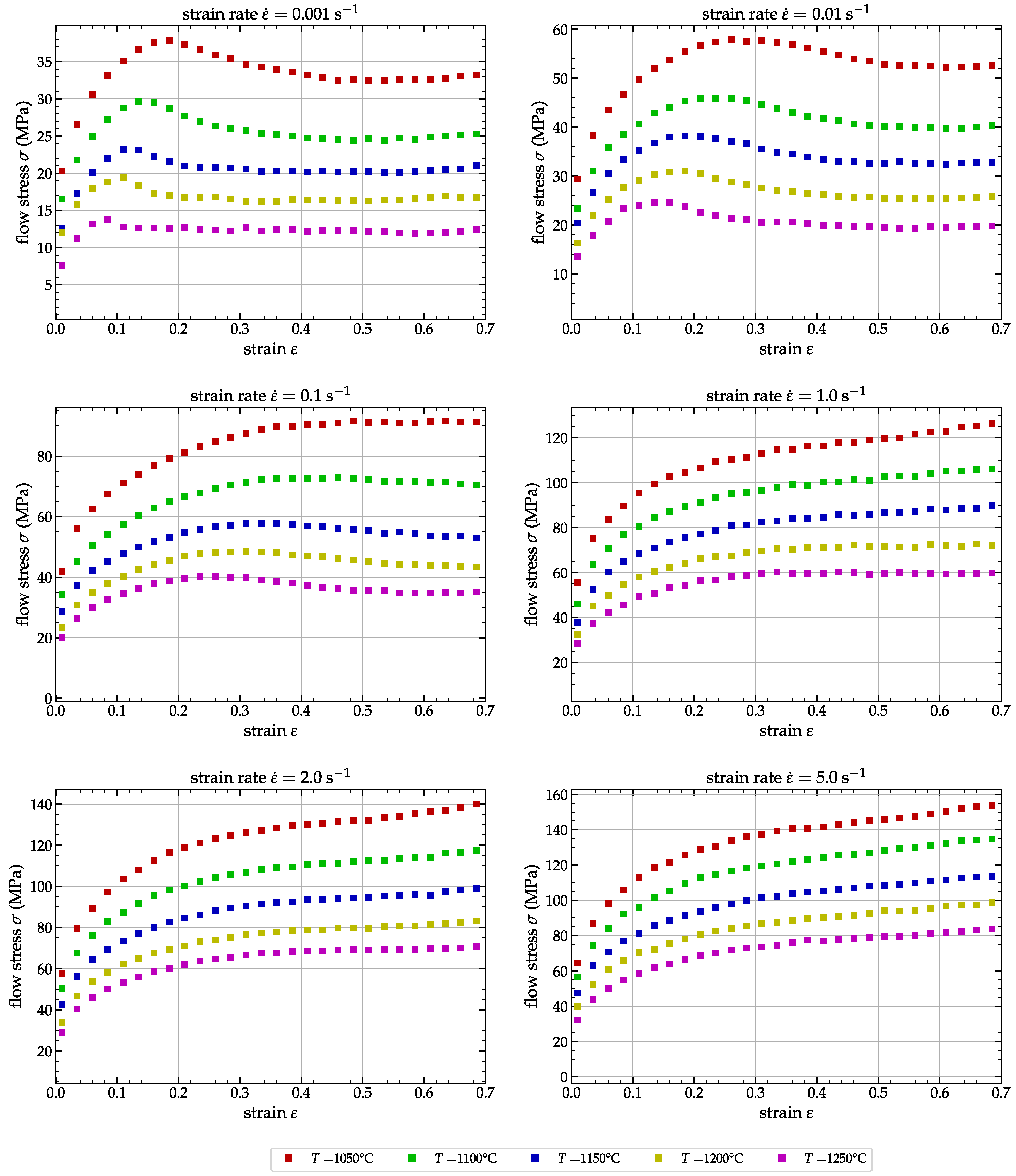
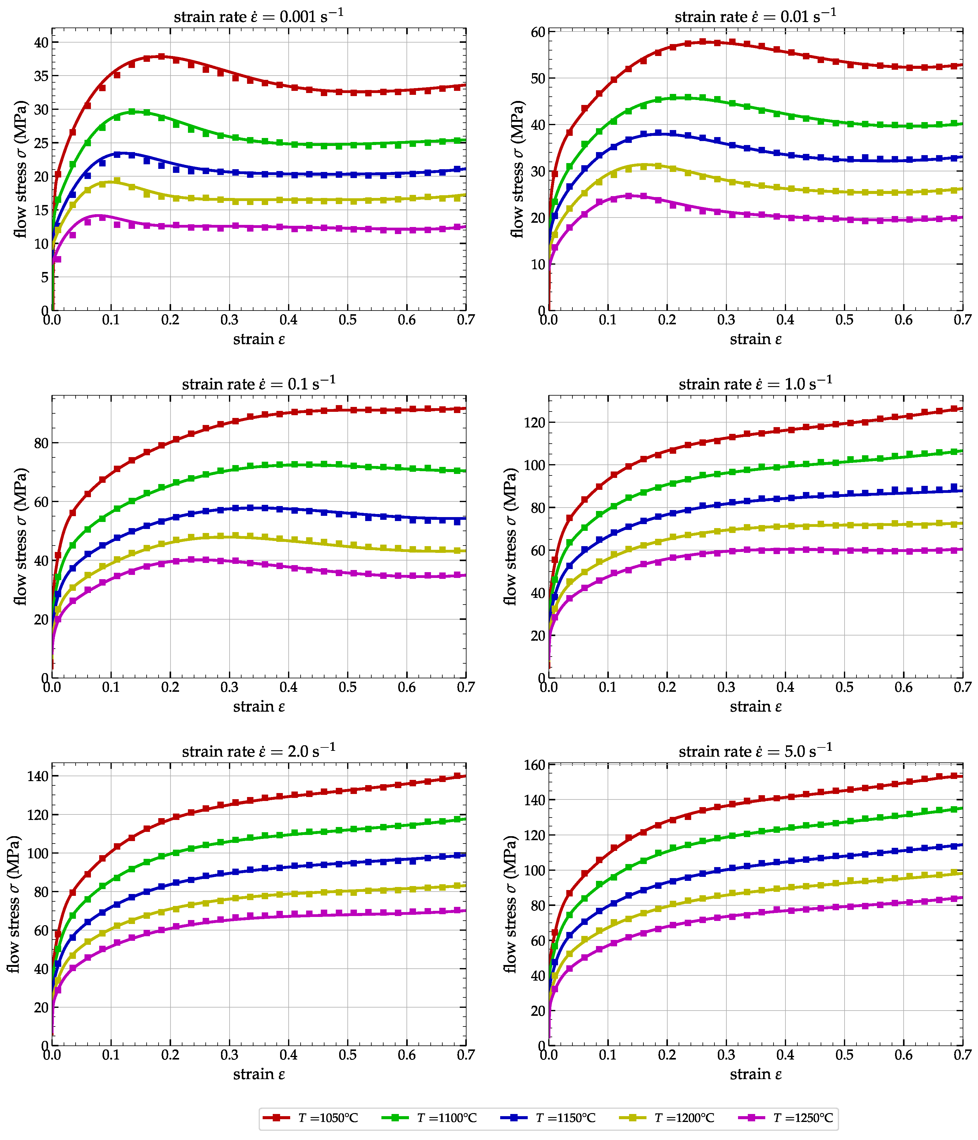
1.2. Experimental Tests and Data

This study uses a medium-carbon steel, type P20, with the chemical composition presented in Table 1.
The experiments used in this study mirror those previously conducted by Tize Mha et al. [14]. These tests involve hot compression on a Gleeble-3800 of P20 steel cylinders with initial dimensions of ϕ 0 = 10 mm and h 0 = 15 mm. Only the most relevant information about those experiments is reported hereafter. In order to have a more complete knowledge about the compression tests conducted during this study, we refer to Tize Mha et al. [14]. Hot compression tests were performed for five temperatures, [ 1050 , 1100 , 1150 , 1200 , 1250 ] and six strain rates [ 0.001 , 0.01 , 0.1 , 1 , 2 , 5 ] s 1 . Figure 1 reports a plot of all 30 strain/stress curves extracted from the experiments.
The experimental database is composed of all strain/stress data for all 30 couples of strain rate and temperature. Each strain/stress curve contains 701 equidistant strains ε = [ 0.0 , 0.7 ] in Δ ε = 0.001 increments. The complete database contains 21,030 quadruplets ( ε , ε . , T and σ ). This dataset will be used here after to identify the ANN flow law parameters depending on the selected hyperparameters of the ANNs.
Section 2 is dedicated to the presentation of the ANN based flow law. The first part is dedicated to a reminder of the basic notions on ANNs, with a section on the choice of activation functions to be used in the formulation. The architecture chosen for the formulation of the flow laws based on a two-hidden-layer network will then be presented, together with the formulation of the derivatives of the output with regard to the input variables. The learning methodology and the results in terms of network performance as a function of the activation functions selected will then be presented. Section 3 is dedicated to the FE simulation of a compression test using the explicit version of Abaqus, integrating the ANN implemented as a user routine in Fortran. The quality of the numerical solution obtained and its performance in terms of computational cost will be analyzed as a function of the network structure. Finally, the last section concerns conclusions and recommendations.

2. Artificial Neural Network Flow Law

As previously proposed by Pantalé et al. [15,16], the employed methodology involves embedding the flow law, defined by a trained ANN, into the Abaqus code as a Fortran subroutine. The ANN is trained using the experiments, as introduced in Section 1, to compute the flow stress σ as a function of ε , ε . and T. Following the training phase, the ANN’s weights and biases are transcribed into a Fortran subroutine, which is then compiled and linked with Abaqus libraries. This integration enables Abaqus to incorporate the thermomechanical behavior by computing the flow stress and its derivatives ( σ / ε , σ / ε . , and σ / T ) essential for the radial-return algorithm within the FE code.

2.1. Artificial Neural Network Equations

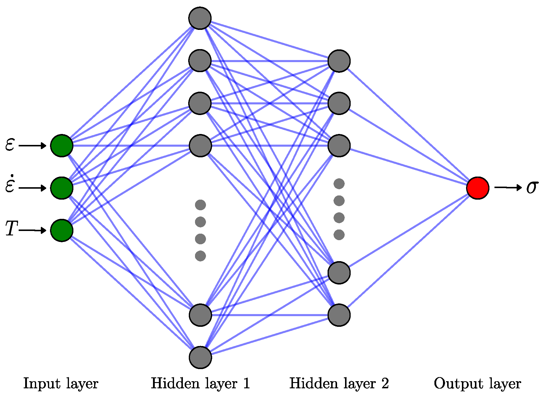
2.1.1. Network Architecture

As illustrated in Figure 2, the ANN used for computing σ from ε , ε . and T is a two hidden layers network.
The input of the neural network is a three component vector noted x . Layer [ k ] , composed of n neurons, computes the weighted sum of the outputs y ^ [ k 1 ] of previous layer [ k 1 ] , composed of m neurons, according the equation:
y [ k ] = w [ k ] · y ^ [ k 1 ] + b [ k ] ,
where y [ k ] are the internal values of the neurons resulting the summation at the layer level [ k ] , w [ k ] is the weights matrix [ n × m ] linking layer [ k ] and layer [ k 1 ] , b [ k ] is the bias vector of layer [ k ] and y ^ [ k 1 ] is the output vector of layer [ k 1 ] result of the activation function defined hereafter.
The number of learning parameters N for any layer [ k ] is the sum of the weights and biases in that layer, expressed as N = n ( m + 1 ) . Following the summation operation outlined in Equation (2), each hidden layer [ k ] produces an output vector y ^ [ k ] computed through an activation function f [ k ] , as defined by the subsequent equation:
y ^ [ k ] = f [ k ] ( y [ k ] ) .
This process is repeated for each hidden layer of the ANN until we reach the output layer where the formulation differ, so that the output s of the neural network is given by:
s = w T · y ^ [ 2 ] + b ,
where w is the vector of the output weights of the ANN and b is the bias associated with the output neuron. As usually done in a regression approach, there is no activation function associated with the output neuron of the network (or some authors consider here a linear activation function).

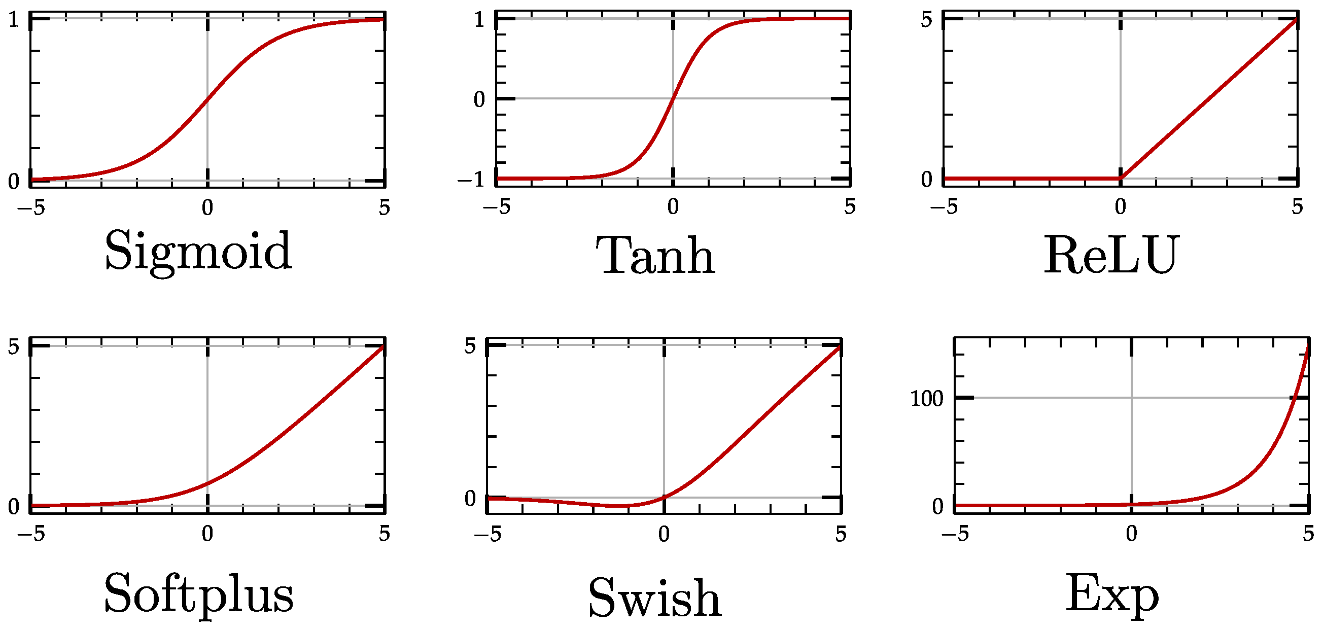
2.1.2. Activation Functions

At the heart of ANNs lies the concept of activation functions, pivotal elements that determine how information is transformed within the neurons. Choosing activation functions is a critical design decision, as these functions greatly influence the network’s capacity to learn and represent complex patterns in data. The selection of activation functions is guided by their distinct properties, including non-linearity, differentiability, and computational efficiency.
In regression ANNs, the choice of activation functions is typically driven by the need to approximate continuous output values rather than class labels. Many studies have been proposed concerning the right activation function to use depending on the physical problem to solve, such as the reviews proposed by Dubey et al. [28] or Jagtap et al. [29]. The activation function is essential for introducing non-linearity into a neural network, allowing it to capture non-linear features. Without this non-linearity, the network would behave like a linear regression model, as emphasized by Hornik et al. [18]. A number of activation functions can be used in neural networks.
In our previous published work [15,16], we have mostly used the Sigmoid activation function for the ANN flow laws. In the present paper, we are going to explore other activation functions and their influence on the final results, up-to the implementation into a FE software. Among the number of activation functions available in the literature, we have selected the six ones reported in Figure 3.
The Sigmoid activation function [30], also known as the logistic activation function, is widely used in ANNs. It was originally developed in the field of logistic regression and later adapted for use in neural networks. It maps any input to an output in the range [ 0 , 1 ] , making it suitable for tasks where the network’s output needs to represent probabilities or values between 0 and 1. The Sigmoid activation function f ( x ) and its derivative f ( x ) are defined by:
f ( x ) = 1 1 + e x and f ( x ) = f ( x ) 1 f ( x ) .
This function has been widely used until the early 1990s. Its main advantage is that it is bounded, while its main drawbacks are the problem of vanishing gradient, a non-centered on zero output and saturation for large input values.
From the 1990s to 2000s, the hyperbolic tangent activation function has been introduced and was preferred to the Sigmoid function for the training of ANNs. The hyperbolic tangent function squashes the output within the range [ 1 , + 1 ] , and its formulation is given by the following equations:
f ( x ) = e x e x e x + e x and f ( x ) = 1 f ( x ) 2 .
This function is useful when the network needs to model data with mean-centered features, as it can capture both positive and negative correlations. The Tanh activation function and the Sigmoid activation function are closely related in the sense that they both introduce non-linearity and squash their inputs into bounded ranges. The evaluation of this activation function requires more CPU time than the Sigmoid function, since we need to compute two exponential functions ( e x and e x ) to evaluate f ( x ) .
ReLU is a classic function in classification ANNs due to its simplicity and computational efficiency, as it involves simple thresholding. It introduces non-linearity and is computationally efficient. It outputs the input if it is positive and zero if it is negative:
f ( x ) = max ( 0 , x ) and f ( x ) = 1 x > 0 0 x 0 .
ReLU mitigates the vanishing gradient problem better than Sigmoid and Tanh, making it suitable for deep networks. It often leads to faster convergence in training deep neural networks. The vanishing gradient for all negative input is the major drawback of the ReLU function.
The Softplus function [31] approximates the ReLU activation function smoothly. It is defined as the primitive of the Sigmoid function and is written:
f ( x ) = log 1 + e x and f ( x ) = 1 1 + e x .
Softplus activation function enhances a more gradual transition from zero than ReLU, and can model positive and negative values. The main drawback is that its computational efficiency is low, since we need to compute two exponential and one logarithmic functions to evaluate f ( x ) and its derivative.
Swish [32] is a smooth and differentiable activation function defined as:
f ( x ) = x 1 + e x and f ( x ) = f ( x ) + 1 f ( x ) 1 + e x .
Swish demonstrates enhanced performance in certain network architectures, particularly when employed as an activation function in deep learning models, and its simplicity and similarity to ReLU facilitate straightforward substitution in neural networks by practitioners. Even if the expression of the Swish function and its derivative seems more complex that the Softplus function presented earlier, the CPU time is lower.
Looking at the shape of the ReLU and Swish functions, apart from those classic activation functions already widely used in ANNs, we propose hereafter to add an extra one, based on the exponential function and simply defined by:
f ( x ) = e x and f ( x ) = f ( x ) .
We found very few papers about the use of the exponential activation function in ANNs, but it has been reported that in specific domains and mathematical modeling tasks, exponential activations can be highly relevant and effective. The idea here is to use the property so that the derivative expression is defined only by the function itself, as well as for the Sigmoid and Tanh, but with the simplest formulation. This will reduce the CPU cost since we need to compute both the function and its derivative for our implementation in the FE code into a very CPU intensive subroutine, due to the explicit integration.
Of course, there is no limitation to the use of alternative activation functions in ANNs, and there exist some much more complicated, such as the one proposed by Shen et al. [33], which is a combination of a floor, an exponential and a step function. Those authors have proven that a three hidden layer with this activation function can approximate any Hölder continuous function with an exponential approximation rate.
In order to compare the different activation functions, all six activation functions presented earlier will be used in the rest of this paper and efficiency, precision of the models and computational cost will be analyzed.

2.1.3. Pre- and Post-Processing Architecture

As we are using activation functions that mitigate vanishing gradients for large values, it is essential to normalize the three inputs and the output within the range of [ 0 , 1 ] to prevent ill-conditioning of the neural network. This range has been chosen because we will use the Sigmoid activation function as one of the six proposed formulations, while this later squashed the output to the lowest range [ 0 , 1 ] .
Concerning the inputs, the range Δ [ ] and minimum [ ] 0 values of the input quantities are very different according to the data presented in Section 1. In our case, the range and minimum values of the strain are Δ ε = 0.7 and ε 0 = 0 , respectively. Concerning the strain rate Δ ε . = 4.999 s 1 and ε . 0 = 0.001 s 1 and concerning the temperature Δ T = 200 and T 0 = 1050 .
As introduced in Pantalé et al. [15], and with regard to considerations concerning the influence of the strain rate over the evolution of the stress, we first substitute log ( ε . / ε . 0 ) for ε . . Then, in a second time, we remap the inputs x i within the range [ 0 , 1 ] , so that the input vector x is calculated from ε , ε . and T using the following expressions:
x = x 1 = ε ε 0 / Δ ε x 2 = log ( ε . / ε . 0 ) [ log ( ε . / ε . 0 ) ] 0 / Δ [ log ( ε . / ε . 0 ) ] x 3 = T T 0 / Δ T ,
where [ ] 0 and Δ [ ] are the minimum and range values of the corresponding field.
The flow stress σ enhances the same behavior with Δ σ = 153.7 MPa and σ 0 = 0 MPa . Therefore, we apply the same procedure as previously presented and the flow stress σ is related to the output s according to the expression:
σ = Δ σ · s + σ 0 .

2.1.4. Derivatives of the Neural Network

As presented in Section 1, in order to implement the ANN as a Fortran routine in Abaqus, we need to compute the three derivatives of σ with respect to t ε , ε . and T. We can compute those derivatives using differentiation of the output with respect to the inputs. As illustrated in Figure 2, we are using here a two hidden layers neural network. Therefore, as Equations (2)–(4) are used to compute y [ k ] and y ^ [ k ] for each hidden layer and the output s from the input vector x of the ANN, we can write the derivative s of a two hidden layers network as follows:
s = w [ 1 ] T · w [ 2 ] T · w T f ( y [ 2 ] ) f ( y [ 1 ] ) ,
where f is the activation function’s derivative introduced by Equations (5)–(10) and ∘ is the Hadamard product (the so-called element-wise product). Because of the pre and post processing of the values introduced in Section 2.1.3, the derivative of the flow stress σ with respect to the inputs ε , ε . and T is then given by:
σ / ε = s 1 · Δ σ / Δ ε σ / ε . = s 2 · Δ σ / ( ε . · Δ ε . ) σ / T = s 3 · Δ σ / Δ T ,
where s i is one of the three components of the vector s defined by Equation (13).
Finally, Equations (2)–(4), (11)–(14) and the requested activation function defined by one of Equations (5)–(10) will be used to implement the ANN as a Fortran subroutine for the Abaqus FE software, as it will be presented in Section 3.1.

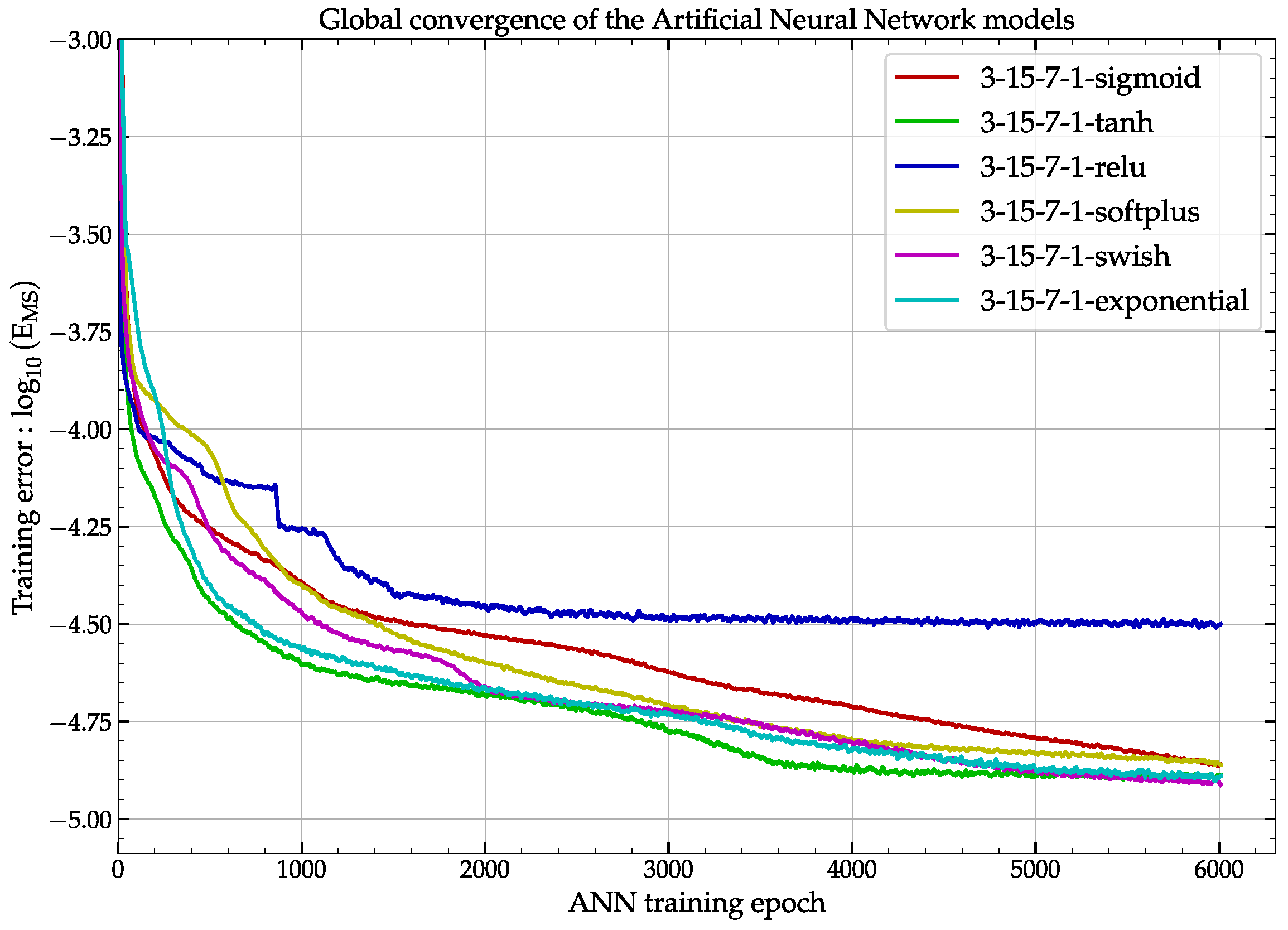
2.2. Training of the ANN on Experimental Data

The Python program, developed with the dedicated library Tensorflow [34], utilized the Adaptive Moment Estimation (ADAM) optimizer [35] and the Mean Square Error for assessing the loss function during the training phase. With regard to our previous publications about ANN constitutive flow law [15], we have made the choice to arbitrarily fix some hyper-parameters of the ANNs, so to use a two hidden layers ANN with 15 neurons for the first hidden layer and 7 neurons for the second hidden layer. There is a total number of 180 trainable parameters to optimize. As we have three inputs and one output, we reference each of the ANNs using the notation 3-15-7-1-act, where act refers the activation function used for the model. All six models underwent parallel training for a consistent number of iterations (6000 iterations, lasting around 1 h), on a Dell PowerEdge R730 server running Ubuntu 22.04 LTS 64-bit, equipped with 96 GB of RAM and 2 Intel Xeon CPU E5-2650 2.20 GHz processors.
Concerning the dataset used for the training of the ANN, as already introduced in the previous sections, this dataset is composed of 21,030 quadruplets ( ε , ε . , T and σ ) acquired during the Gleeble experiments described in Section 1.2. A chunk of 75 % of the dataset is used for training while the rest is used for the test during the training of the ANN. All details about this procedure can be found in Pantalé [36] where the interested reader can download the source, data and results of this training program. Regarding the training procedure, specifically the starting point, all models are initialized with precisely identical weights and biases. However, due to different activation functions, the initial solution varies from one model to another.
Error evaluation of the models uses the Mean Square Error ( E MS ), the Root Mean Square Error ( E RMS ) and the Mean Absolute Relative Error ( E MAR ) given by the following equations:
E MS = 1 N i = 1 N i e i 2 E RMS ( MPa ) = E MS E MAR ( % ) = 1 N i = 1 N i i e i e × 100 ,
where N is the total number of points for the computation of those errors, i is the ith output value of the ANN, and i e is the corresponding experimental value.
Figure 4 shows the evolution of the common logarithm of the Mean Square Error, i.e., log 10 ( E MS ) , of the output s of the ANN during the training, evaluated using only the test data ( 25 % of the dataset).
By examining this figure, we can assess and compare the convergence rates of various ANNs, concluding that a stable state was more-or-less achieved for all analyzed ANNs after 6000 iterations. As expected, the ReLU activation function gives the worst results with a final value of E MS = 32 × 10 6 , mainly due to the low number of neurons and the fact that this function is a piecewise linear function and not able to efficiently approximate the nonlinear behavior of the material. The other five activation functions enhance more or less the same behavior. The final value of the E MS is pretty much the same for all of them, and around E MS = 12 × 10 6 . Table 2 reports the results of the training phase, the errors reported in this Table are computed using the whole dataset (both train and test parts).
From the data, it is evident that all models require approximately the same training time to complete the specified number of iterations, with the complexity of activation functions influencing this duration; notably, the training time is a bit greater for Swish and Softplus functions compared to ReLU. We also reported in this table the real values of the E RMS and E MAR concerning the flow stress σ using the whole experimental database. From the latter, we can see that the E RMS is about 0.6 MPa for all activation functions except the ReLU one, where the value is above 0.8 MPa . Concerning the E MAR , the value of all models is around 1 % , while it is more than 2 % for the ReLU function. Of the six activation functions, the Exponential function gives the best results in terms of solution quality, while the ReLU function gives the worst, as reported by computing the global error using the following expression Δ E = E RMS 2 + E MAR 2 . But we must note that the results of all models, except the ReLU one are very close at the end of the training stage, as illustrated in Figure 4 and Table 2. Depending on when the train is stopped, a particular model may yield the best performance due to the varying slopes of convergence among the models.
Figure 5 reports a comparison of the experimental stress acquired during the Gleeble compression tests (reported as dots in Figure 5) and the predicted stress σ using the ANN for the strain rate ε . = 1 s 1 .
From this observation, we can infer that all ANNs effectively replicate the experimental results, except for the ReLU activation function. In the case of ReLU, as depicted in Figure 5, the predicted flow stress exhibits a piecewise linear behavior.
Of the six activation functions introduced, as detailed in Section 2.1.2, the exponential function stands out due to its unique features. The computation of the function and its derivative in a single step necessitates only one evaluation of the exponential function, as indicated by f ( x ) = f ( x ) in Equation (10). If we analyze the results reported in Table 2 and Figure 5 concerning the exponential activation function, we can see that this one has a E RMS = 0.688 MPa , E MAR = 1.176 % and the global behavior of the flow stress for ε . = 1 s 1 is similar to the Sigmoid, Tanh, Swish or Softplus functions.
In terms of the global performance of the 3-15-7-1-exp ANN, Figure 6 reports the comparison of the experimental data (dots) and the ANN flow stress for all strain rates and temperatures defined in Section 1.2.
We can see that over the whole temperatures T and strain rates ε . , the performance of the model based on an exponential function is very good overall. This model will therefore be retained for the remainder of the comparative study.
It is well known that artificial neural networks are able to interpolate data correctly within their learning domain, but behave unsatisfactorily when we wish to evaluate results outside the boundaries of this learning domain. The ANNs developed in this study follow this general rule, but with different degrees of progress depending on the nature of the activation function used. In order to test the extreme limits of the proposed networks, Figure 7 shows the comparison of predicted values according to the nature of the network for conditions globally outside the learning limits.
We selected the worst case, multiplied the strain range by 2 (up to ε = 1.4 ), multiplied the strain rate by 2 ( ε . = 10 ) and lowered the temperature to T = 1000 . Figure 7 shows the evolution of the flow stress predicted by the six models. In Figure 7, top left, when deformation alone is extended, we can see that all six models correctly predict the flow stress evolution over the interval ε = [ 0 , 0.7 ] , whereas they diverge beyond a deformation of ε = 0.7 . The behavior of the different models is highly variable, and overall, only the Sigmoid and Tanh models show a physically consistent trend. The model with an exponential activation function behaves catastrophically outside the learning range, due to the very nature of the exponential function. When deformation and temperature are out of range (top right), behavior is consistent below ε = 0.7 and divergent beyond. Again, only the Sigmoid and Tanh models show a physically consistent trend above ε = 0.7 . When strain and strain rate are out of range (bottom left in Figure 7), the behavior is consistent below ε = 0.7 , while diverging above ε = 0.7 . The values given by the exponential model are out of range for all strain values. Finally, when all inputs are out of range (bottom right), the behavior is consistent and identical, except for the ReLU model below ε = 0.7 . It is divergent above ε = 0.7 , and consistent only for the Sigmoid and Tanh models.
We can therefore conclude from this extrapolation study that it is important to remain as far as possible within the limits of the neural network’s learning domain if the results are to be physically admissible. Furthermore, from these analyses, it appears that only the Sigmoid and Tanh models are capable of physically admissible prediction of the flow stress values outside the learning domain. This is due in particular to the double saturation of the tanh and sigmoid functions, as illustrated in Figure 3, when the input values are outside the usual limits.

3. Numerical Simulations Using the ANN Flow Law

Now that the flow stress models have been defined, trained and the results analyzed in terms of their relative performance in reproducing the experimental behavior recorded during compression tests on Gleeble, we will now numerically implement these models in Abaqus as a user routine in Fortran in order to perform numerical simulations. Following training, the optimized internal parameters of the ANNs are saved in HDF5 [37] files. Subsequently, a Python program is responsible for reading these files and generating the Fortran 77 subroutine for Abaqus.
The implementation of a user flow law in Abaqus FE code, specifically using the Explicit version, involves programming the computation of the stress tensor σ 1 based on the stress tensor at the beginning of the increment σ 0 and the strain increment Δ ε . A predictor/corrector algorithm, such as the radial-return integration scheme [7], is typically employed. For detailed implementations, Ming et al. [12] discusses the Safe Newton integration scheme, and Liang et al. [13] focuses on an application related to the Arrhenius flow law. During the corrector phase, the flow stress σ must be evaluated at the current integration point as a function of ε , ε . , and T. This process involves solving a non-linear equation defining the plastic corrector expression and computing three derivatives of the flow stress: σ / ε , σ / ε . , and σ / T . Typically, the subroutine VUHARD in the Abaqus explicit is responsible for computing these quantities, and its implementation depends on the structure and activation functions of the ANN.

3.1. Numerical Implementation of the ANN Flow Law

In order to have a better understanding of the implementation of the VUHARD subroutine, we are going to detail the computation of the flow stress and the three derivatives in one step as a function of the triplet of input values ε , ε . , T. We suppose that the current input is stored in a three components vector ξ T = ε , log ( ε . / ε . 0 ) , T . We also suppose that the minimum and range values of the inputs, used during the learning phase, are stored in two vectors ξ 0 and Δ ξ , respectively.
  • We first use Equation (11) to compute the vector x where all components of ξ will be remapped within the range [ 0 , 1 ] :
    x = ξ ξ 0 Δ ξ ,
    where ⊘ is the Hadamard division operator.
  • Conforming to Equation (2), we compute the vector:
    y [ 1 ] = w [ 1 ] · x + b [ 1 ] .
  • Then, from Equation (3) and the expression of the activation function in the first layer and defined by one of the Equations (5)–(10), we compute the vector:
    y ^ [ 1 ] = f [ 1 ] ( y [ 1 ] ) .
  • We repeat the process for the second layer, so that we compute the vectors:
    y [ 2 ] = w [ 2 ] · y ^ [ 1 ] + b [ 2 ] ,
    and:
    y ^ [ 2 ] = f [ 2 ] ( y [ 2 ] ) .
  • From Equations (4) and (12), we compute the flow stress σ using the following equation:
    σ = Δ σ · w T · y ^ [ 2 ] + b + σ 0 .
  • Then, we can compute in a single step the three derivatives σ from Equation (13) with the following expression:
    σ = Δ σ · w [ 1 ] T · w [ 2 ] T · w T f ( y [ 2 ] ) f ( y [ 1 ] ) Δ ξ σ 2 : = σ 2 / ε . ,
    where the expression used for f ( ) changes depending on the activation function used.
As an illustration the corresponding implementation using Python of those equations is proposed in Appendix A. A dedicated Python program is used to translate those equations into a Fortran 77 subroutine. During the translation phase, all functions corresponding to array operators, as matrix–matrix multiplications or element-wise operations, are converted into unrolled loops (explicitly written), all values of the ANNs parameters are explicitly written as data at the beginning of the subroutine, so that the a 3-15-7-1-exp Fortran routine consist of more than 400 lines of code. A small extract of the corresponding VUHARD subroutine is presented in Figure A2 in Appendix B. All full source files of the six VUHARD subroutines is available in the Software Heritage Archive [36].
The Fortran subroutine is compiled with double precision directive using the Intel Fortran 14.0.2 compiler on a Ubuntu 22.04 server and linked to the main Abaqus explicit executable.

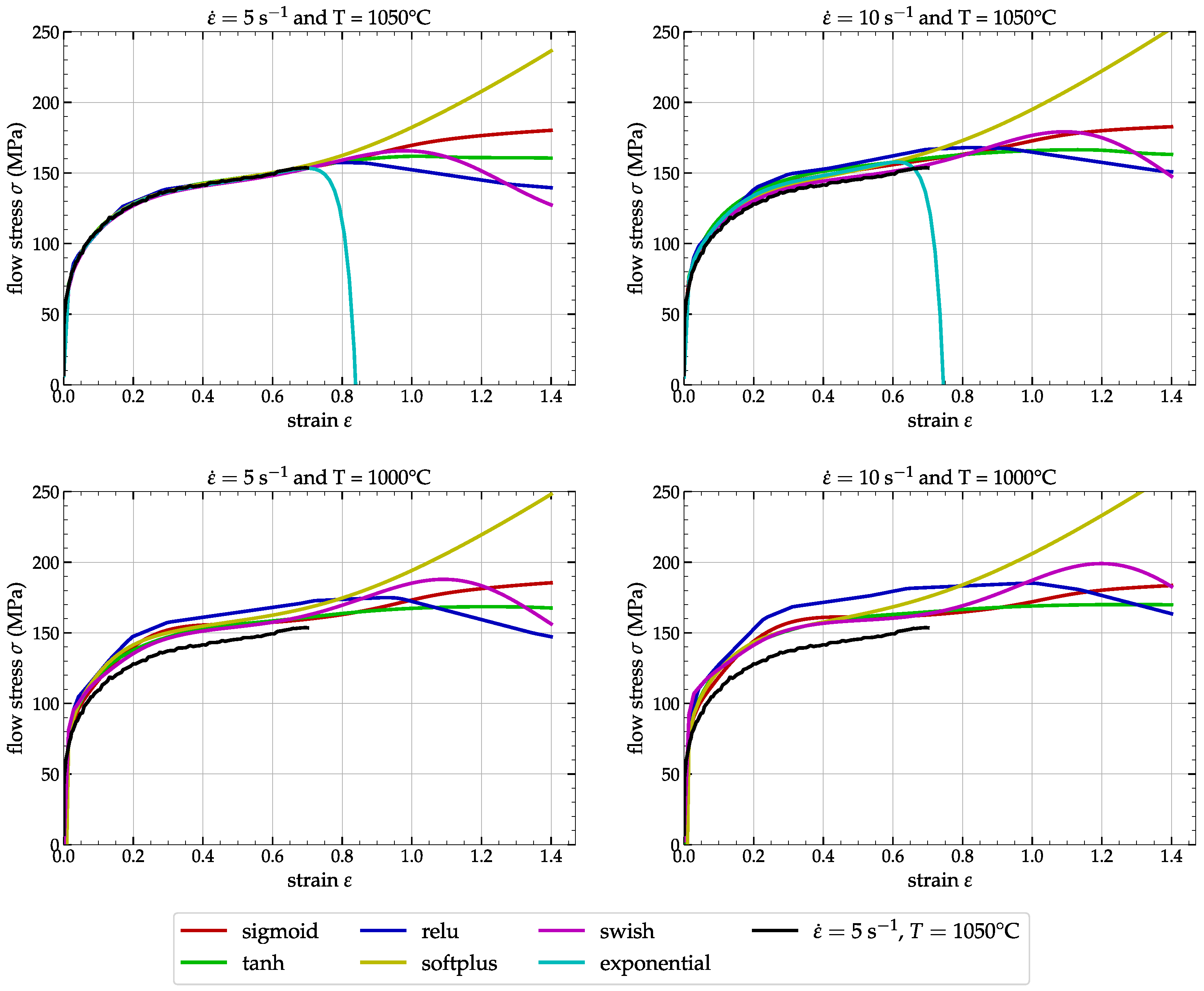
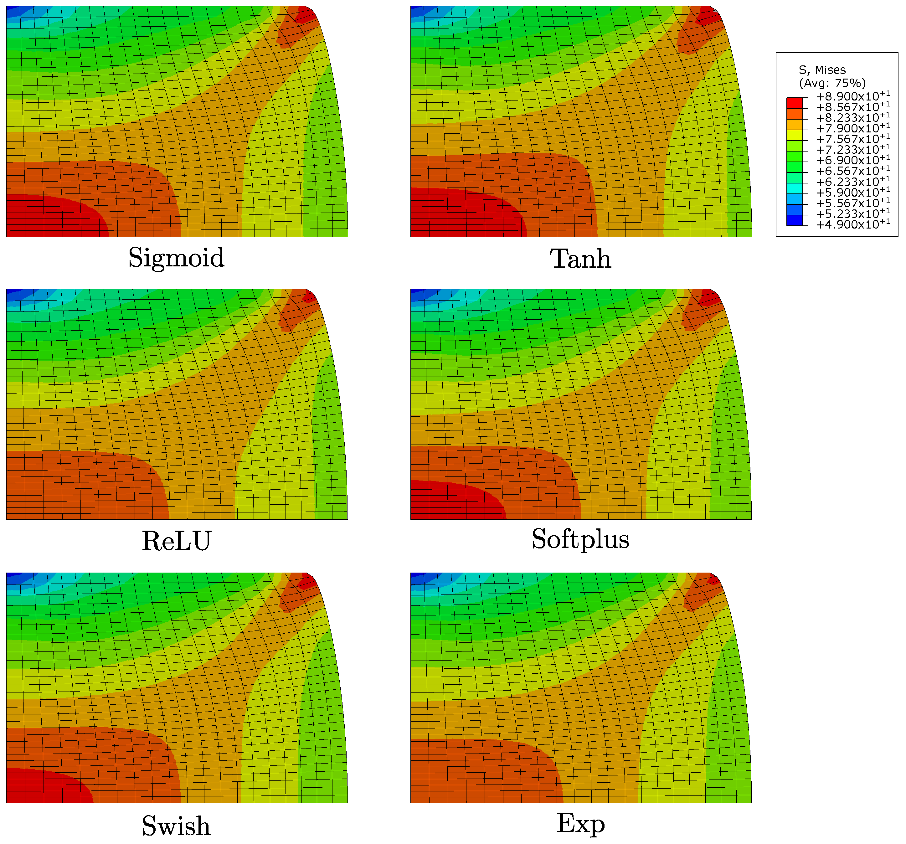
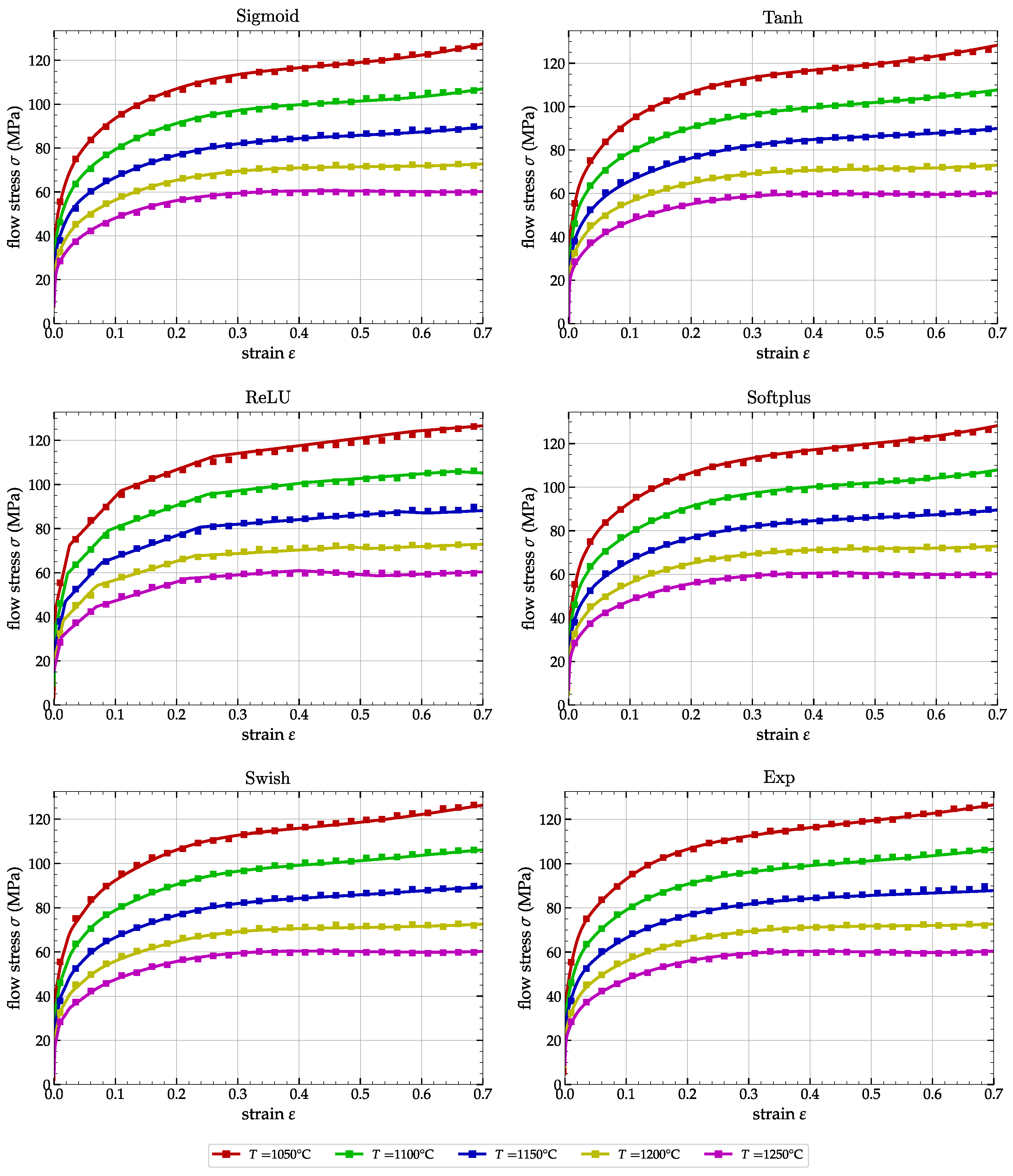
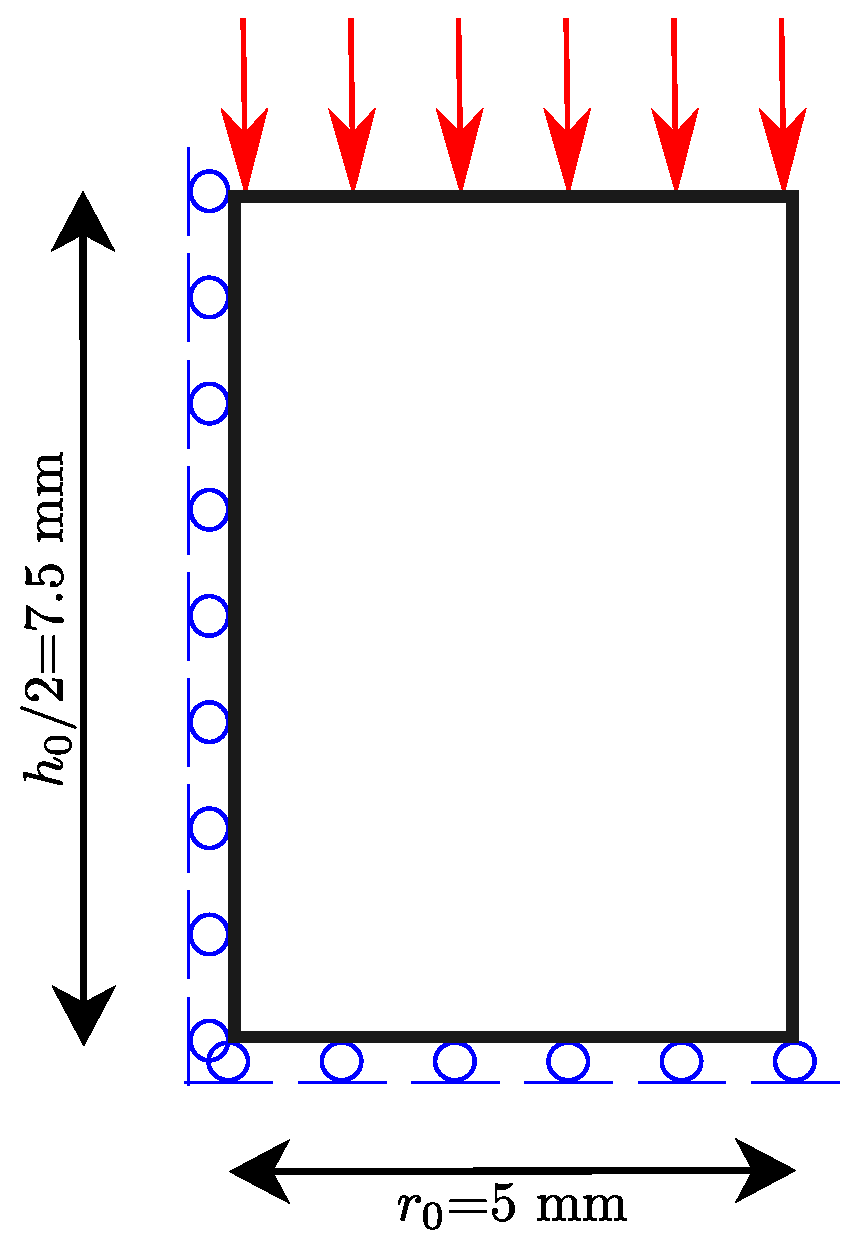
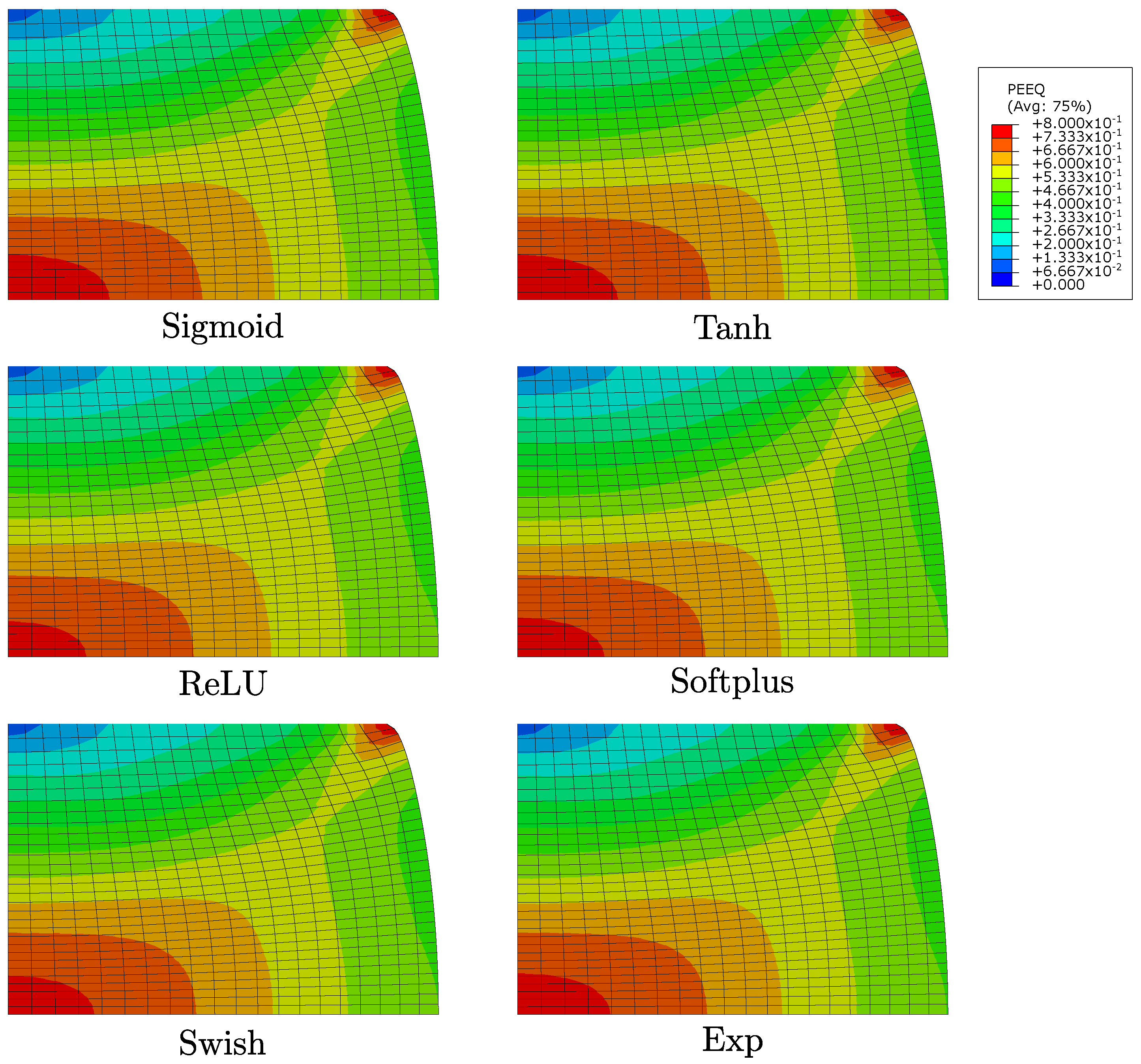
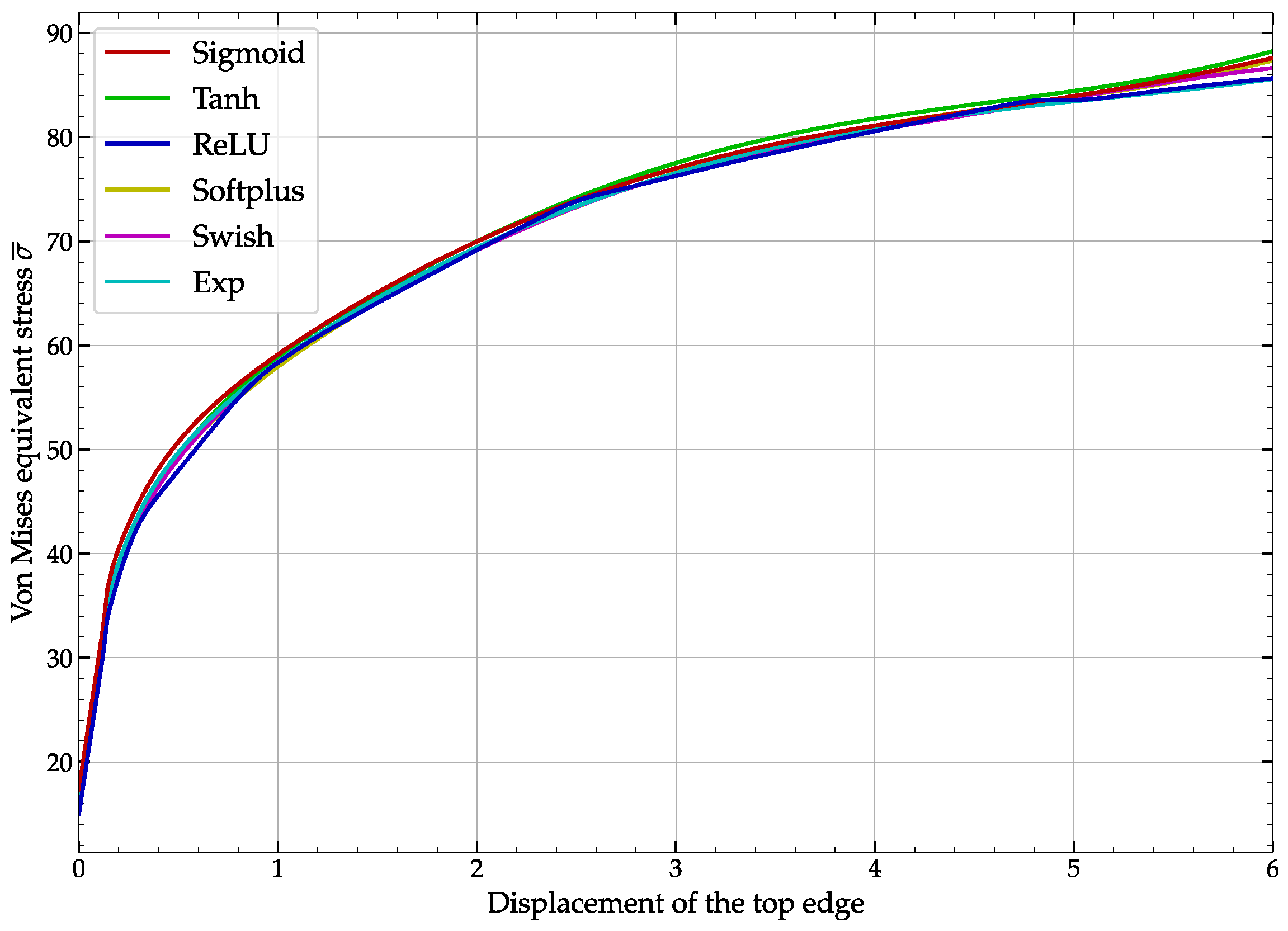
3.2. Numerical Simulations and Comparisons

To compare the influence of choosing different activation functions on the numerical results using Abaqus explicit, we have made the choice to model the compression test presented earlier in Section 1.2. We consider therefore a medium-carbon steel, type P20 cylinder in compression with the initial dimensions ϕ 0 = 10 mm and h 0 = 15 mm as reported in Figure 8, where only the superior half part of cylinder is represented, as the solution is symmetrical on either side of a cutting plane located halfway up the cylinder.
At the end of the process, the height of the cylinder is h f = 9 mm, i.e., the top edge displacement is d = 6 mm and the reduction is 40 % of the total height. The displacement is applied with a constant speed and the simulation time is fixed to t = 1 s, i.e., the strain rate is in the range ε . = [ 0.5 , 1.0 ] s 1 at the center of the specimen. The mesh comprises 600 axis-symmetric thermomechanical quadrilateral finite elements (CAX4RT) featuring four nodes and reduced integration. It includes 20 elements along the radial direction and 30 elements along the axis. The element size is 0.25 × 0.25 mm 2 . Only reduced integration is available in Abaqus explicit for an axis-symmetric structure. The anvils are modeled as two rigid surfaces and a Coulomb friction law with μ = 0.15 is used. To reduce the computing time, a global mass scaling with a value of M s = 1000 is used. The initial temperature of the material is set to T 0 = 1150 , and we use an explicit adiabatic solver for the simulation of the compression process. All simulations are performed using the 2022 version of the Abaqus explicit solver on the same computer as the one used for the learning of the ANNs in Section 2.2. Simulations are performed with the double precision version of the solver without any parallelization directive to better compare the CPU times.
Figure 9 shows, at the end of the simulation (when the displacement of the top edge is d = 6 mm), a comparison of the equivalent plastic strain ε ¯ p contourplot for the six activation functions.
From the latter, we can clearly see that all activation functions gives almost the exact same results and the choice of any of the available ANN has no influence on the values and isovalues contourplot reported in Figure 9.
Figure 10 shows a comparison of the von Mises equivalent stress σ ¯ contourplot.
In this figure, we can see that the solutions differ slightly both in terms of maximum stress value and stress isovalues distribution.
In order to compare the different models quantitatively, Table 3 reports the values of the plastic strain ε ¯ p , the von Mises equivalent stress σ ¯ and the temperature T for the element located at the center of the specimen at the end of the simulation.
From the values reported in this table, we can see that the models differ a little concerning the equivalent stress (below 1 % ), the equivalent plastic strain (below 1 % ) and the temperature (below 0.02 % ). It is important to note that one origin of the differences between the models comes from the fact that in the end of the simulation, the plastic strain ε ¯ p is greater than 0.7 , so the model has to extrapolate the yield stress with respect to the data used for the training phase. This increases the discrepancy between the models, since each extrapolates the results from the training domain differently with respect to its internal formulation.
In Table 3, we also have reported the number of increments N i n c needed to complete the simulation along with the total CPU time. We remark that the number of increment varies from one activation function to another one, since the convergence of the model differ because it takes into account the stress in the computation of the stable time increment. From these two, we can calculate the number of increments performed per second and propose a classification from the fastest to the slowest ANN, where ReLU is the fastest (with 2353 iteration per second) and Softplus is the slowest (with 1200 iteration per second) of the proposed models (two times slower than the ReLU one). Those results are directly linked to the complexity of the expression of the activation function and its derivative as introduced in Section 2.1.2. For example, we can note that a simulation using the Sigmoid activation function requires 1,092,001 increments and the model contains 400 under integrated CAX4RT elements; therefore, we will have 436,800,400 computations of the code presented in Figure A3. From those results, we can note that, as expected, the Exp activation function is very efficient in terms of CPU computation time (with 1996 iteration per second) as it is just second after the very light ReLU function, but gives quite good results as reported in Table 3, which is not the case for the ReLU function.
Figure 11 shows the evolution of the von Mises stress vs. displacement of the top edge for the center of the cylinder for all activation functions.
From this later, we can see that all activation functions give almost the same results, while the ReLU enhances a piecewise behavior due to its formulation and the low number of neurons used for the ANN. This behavior has an influence on the precision of the ANN flow law, and we suggest avoiding the use of the ReLU activation function in this kind of application. Any other type of activation function give quite good results for this application, while among them, the use of the Exp activation function gives accurate results and minimum computation time for numerical applications.

4. Conclusions and Major Remarks

In this paper, several ANN-based flow laws for thermomechanical simulation of the behavior of a P20 medium-alloy steel have been identified. These six laws exhibit distinctions solely in the choice of their activation functions, while maintaining a uniform architectural framework characterized by consistent specifications regarding the quantity of hidden layers and the number of neurons present on each of these hidden layers. In addition to the five classic activation functions (Sigmoid, Tanh, ReLU, Softplus and Swift), in this paper, we proposed the use of the Exp (exponential) function as an activation function, although this is almost never used in neural network formulations. The expressions of the activation functions and their derivatives were used in the neural network writing formalism to calculate the derivatives of σ with respect to ε , ε . and T.
Comparison of the ANNs results (in terms of flow stress σ ) with experiments have shown that all five activation functions, with the exception of the ReLU function, give very good results, far superior to those obtained conventionally using formalisms based on analytical flow laws from the literature, such as the Johnson–Cook, Arrhenius or Zerilli–Armstrong models [14]. To improve the extrapolation ability of the models, it is recommended to use the Sigmoid and Tanh activation functions. These functions can effectively squash out of bounds values, giving the artificial neural network a more realistic behavior beyond the training bounds.
Based on the equations describing the mathematical formulation of an ANN with two hidden layers, and depending on the nature of these activation functions, we have implemented these constitutive laws in the form of a Fortran 77 subroutine for Abaqus explicit. The same approach can also be used to write a UHARD routine enabling the same flow laws to be used in Abaqus standard.
Numerical results obtained from a compression test on a metal cylinder using the Abaqus explicit code have shown that neural network behavior models give very satisfactory results, in line with experimental tests. The Exp activation function, which is rarely used in the formulation of artificial neural networks, showed very good results (in agreement with more complex models such as Tanh), while enabling the code user to benefit from the efficiency and ease of implementation of an exponential function. These results are satisfactory insofar as the inputs remain entirely within the model’s learning domain, since the extrapolation capabilities of the network based on the exponential function are very limited. We then obtain results equivalent in terms of solution quality to sigmoid or tanh-type formulations, while having computation times comparable to a ReLU function.
Overall, this study concludes by recommending the use of the sigmoid activation function for the development of flow laws, since it gives very good results in the identification domain, allows us to leave the learning domain with a behavior that is certainly biased, but physically admissible, and offers very good performance in terms of simulation time when implemented in a finite element code. This study emphasizes the valuable impact of neural network-derived flow laws for numerical finite element simulation executed with a commercial FE code like Abaqus.

Funding

This research received no external funding.

Data Availability Statement

Source files of the numerical simulations and the ANN flow laws are available from [36].

Acknowledgments

The author thanks the team of Mohammad Jahazi from the Ecole Technique Supérieure de Montréal, Canada, for providing the experimental data used in Section 1.2.

Conflicts of Interest

The author declares no conflict of interest.

Abbreviations

The following abbreviations are used in this manuscript:
ANNArtificial Neural Network
CAX4RTAbaqus 4 nodes axis-symmetric thermomechanical element
CPUCentral processing unit
FEFinite Element
UHARDAbaqus standard user subroutine
VUHARDAbaqus explicit user subroutine

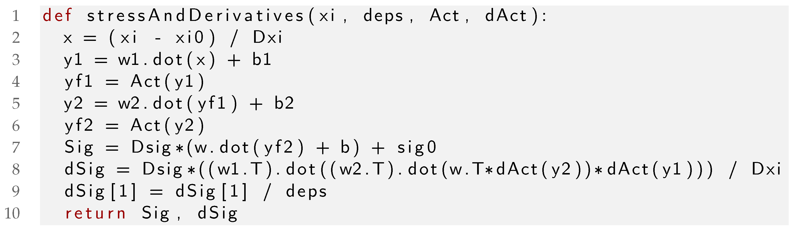
Appendix A. Python Code to Compute Stress and Derivatives

The implementation using Python of Equations (16) to (22) is proposed in Figure A1, where the arguments of the function stressAndDerivatives are xi for the ξ vector, deps for ε . , Act for the activation function and dAct for its derivative.
Figure A1. Python function to compute the flow stress and the derivative vector.
Algorithms 16 00537 g0a1
The network architecture is defined by the numpy arrays w1, w2, w, b1, b2 and b, which are global variables in the proposed piece of code. The other variables xi0, Dxi, sig0 and Dsig correspond to the quantities ξ 0 , Δ ξ , σ 0 and Δ σ , respectively.
Line 2 in Figure A1 corresponds to Equation (16). Lines 3 and 4 correspond to Equations (17) and (18) and concern the first hidden layer, while lines 5 and 6 correspond to Equations (19) and (20) and concern the second hidden layer. Finally, line 7 computes the flow stress σ conforming to Equation (21) and lines 8 and 9 compute the three derivatives of the flow stress conforming to Equation (22). The stress Sig and the three derivatives array dSig are returned as a tuple at line 10.

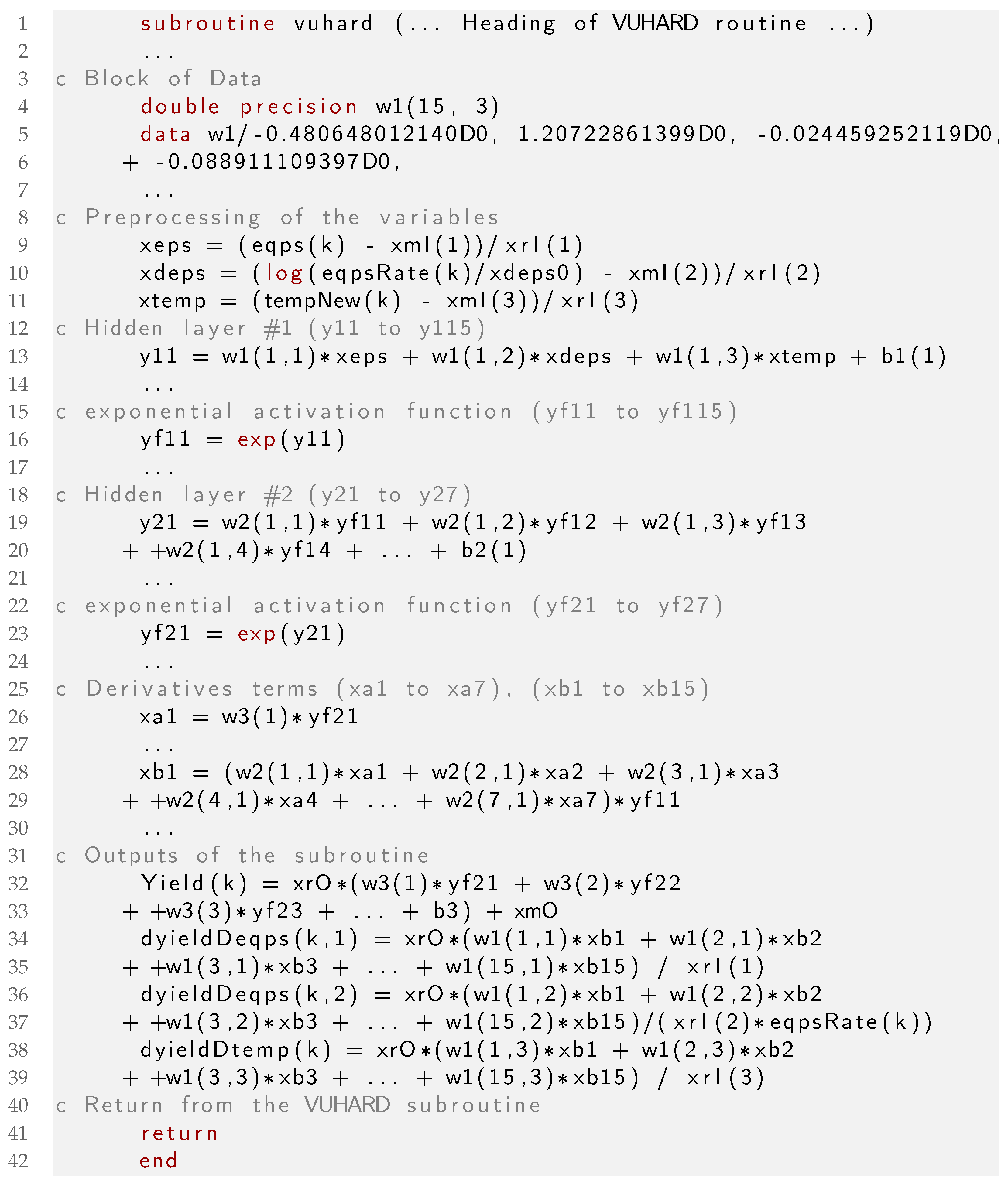
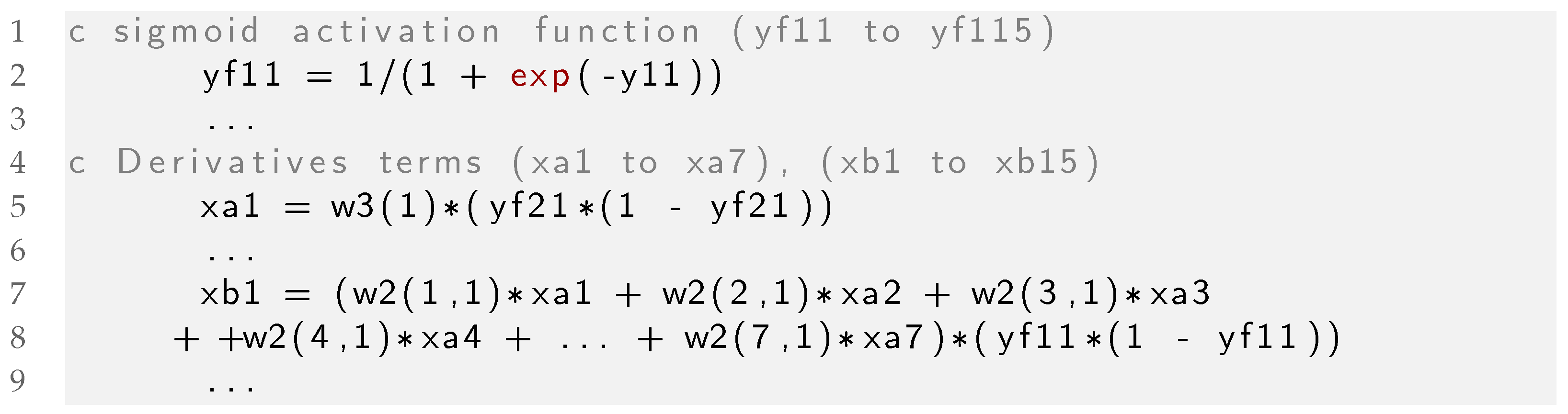
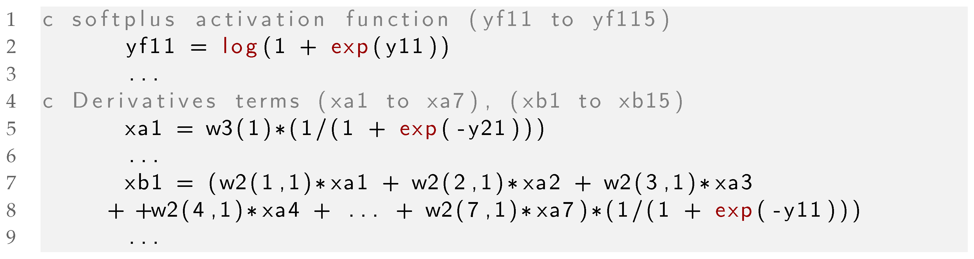
Appendix B. Fortran 77 Subroutines to Implement the ANN Flow Law

A portion of the Fortran 77 code defining the numerical implementation of the VUHARD routine for Abaqus Explicit is presented in Figure A2. The complete source codes for the flow laws corresponding to the six activation functions can be found in the Software Heritage archive [36]. In Figure A2, the ‘…’ symbols denote a continuation of the code that is not transcribed here due to space constraints in the figure for the sake of conciseness.
Depending on the kind of activation function used, some lines differ from one version to the other one, such as the definitions of the activation functions (see line 16 in Figure A2) and the expressions of the internal variables xa and xb (see lines 26 and 28 in Figure A2).
Figure A3 shows the declaration of the Sigmoid activation function and its derivative as defined by Equation (5), while Figure A4 shows the same part of the code with the use of the Softplus activation function as defined by Equation (8).
Figure A2. Part of the VUHARD Fortran 77 subroutine for the ANN flow law and the exponential activation function.
Algorithms 16 00537 g0a2
Figure A3. Part of the VUHARD Fortran 77 subroutine with the Sigmoid activation function.
Algorithms 16 00537 g0a3
Figure A4. Part of the VUHARD Fortran 77 subroutine with the Softplus activation function.
Algorithms 16 00537 g0a4

References

  1. Abaqus. Reference Manual; Hibbitt, Karlsson and Sorensen Inc.: Providence, RI, USA, 1989. [Google Scholar]
  2. Lin, Y.C.; Chen, M.S.; Zhang, J. Modeling of flow stress of 42CrMo steel under hot compression. Mater. Sci. Eng. A 2009, 499, 88–92. [Google Scholar] [CrossRef]
  3. Bennett, C.J.; Leen, S.B.; Williams, E.J.; Shipway, P.H.; Hyde, T.H. A critical analysis of plastic flow behaviour in axisymmetric isothermal and Gleeble compression testing. Comput. Mater. Sci. 2010, 50, 125–137. [Google Scholar] [CrossRef]
  4. Kumar, V. Thermo-mechanical simulation using gleeble system-advantages and limitations. J. Metall. Mater. Sci. 2016, 58, 81–88. [Google Scholar]
  5. Yu, D.J.; Xu, D.S.; Wang, H.; Zhao, Z.B.; Wei, G.Z.; Yang, R. Refining constitutive relation by integration of finite element simulations and Gleeble experiments. J. Mater. Sci. Technol. 2019, 35, 1039–1043. [Google Scholar] [CrossRef]
  6. Kolsky, H. An Investigation of the Mechanical Properties of Materials at very High Rates of Loading. Proc. Phys. Soc. Sect. B 1949, 62, 676–700. [Google Scholar] [CrossRef]
  7. Ponthot, J.P. Unified Stress Update Algorithms for the Numerical Simulation of Large Deformation Elasto-Plastic and Elasto-Viscoplastic Processes. Int. J. Plast. 2002, 18, 36. [Google Scholar] [CrossRef]
  8. Johnson, G.R.; Cook, W.H. A Constitutive Model and Data for Metals Subjected to Large Strains, High Strain Rates, and High Temperatures. In Proceedings of the 7th International Symposium on Ballistics, The Hague, The Netherlands, 19–21 April 1983; pp. 541–547. [Google Scholar]
  9. Zerilli, F.J.; Armstrong, R.W. Dislocation-mechanics-based constitutive relations for material dynamics calculations. J. Appl. Phys. 1987, 61, 1816–1825. [Google Scholar] [CrossRef]
  10. Jonas, J.; Sellars, C.; Tegart, W.M. Strength and structure under hot-working conditions. Metall. Rev. 1969, 14, 1–24. [Google Scholar] [CrossRef]
  11. Gao, C.Y. FE Realization of a Thermo-Visco-Plastic Constitutive Model Using VUMAT in Abaqus/Explicit Program. In Computational Mechanics; Springer: Berlin/Heidelberg, Germany, 2007; p. 301. [Google Scholar]
  12. Ming, L.; Pantalé, O. An Efficient and Robust VUMAT Implementation of Elastoplastic Constitutive Laws in Abaqus/Explicit Finite Element Code. Mech. Ind. 2018, 19, 308. [Google Scholar] [CrossRef]
  13. Liang, P.; Kong, N.; Zhang, J.; Li, H. A Modified Arrhenius-Type Constitutive Model and its Implementation by Means of the Safe Version of Newton–Raphson Method. Steel Res. Int. 2022, 94, 2200443. [Google Scholar] [CrossRef]
  14. Tize Mha, P.; Dhondapure, P.; Jahazi, M.; Tongne, A.; Pantalé, O. Interpolation and extrapolation performance measurement of analytical and ANN-based flow laws for hot deformation behavior of medium carbon steel. Metals 2023, 13, 633. [Google Scholar] [CrossRef]
  15. Pantalé, O.; Tize Mha, P.; Tongne, A. Efficient implementation of non-linear flow law using neural network into the Abaqus Explicit FEM code. Finite Elem. Anal. Des. 2022, 198, 103647. [Google Scholar] [CrossRef]
  16. Pantalé, O. Development and Implementation of an ANN Based Flow Law for Numerical Simulations of Thermo-Mechanical Processes at High Temperatures in FEM Software. Algorithms 2023, 16, 56. [Google Scholar] [CrossRef]
  17. Minsky, M.L.; Papert, S. Perceptrons; An Introduction to Computational Geometry; MIT Press: Cambridge, UK, 1969. [Google Scholar]
  18. Hornik, K.; Stinchcombe, M.; White, H. Multilayer Feedforward Networks Are Universal Approximators. Neural Net. 1989, 2, 359–366. [Google Scholar] [CrossRef]
  19. Gorji, M.B.; Mozaffar, M.; Heidenreich, J.N.; Cao, J.; Mohr, D. On the Potential of Recurrent Neural Networks for Modeling Path Dependent Plasticity. J. Mech. Phys. Solids 2020, 143, 103972. [Google Scholar] [CrossRef]
  20. Jamli, M.; Farid, N. The Sustainability of Neural Network Applications within Finite Element Analysis in Sheet Metal Forming: A Review. Measurement 2019, 138, 446–460. [Google Scholar] [CrossRef]
  21. Lin, Y.; Zhang, J.; Zhong, J. Application of Neural Networks to Predict the Elevated Temperature Flow Behavior of a Low Alloy Steel. Comput. Mater. Sci. 2008, 43, 752–758. [Google Scholar] [CrossRef]
  22. Stoffel, M.; Bamer, F.; Markert, B. Artificial Neural Networks and Intelligent Finite Elements in Non-Linear Structural Mechanics. Thin-Walled Struct. 2018, 131, 102–106. [Google Scholar] [CrossRef]
  23. Stoffel, M.; Bamer, F.; Markert, B. Neural Network Based Constitutive Modeling of Nonlinear Viscoplastic Structural Response. Mech. Res. Commun. 2019, 95, 85–88. [Google Scholar] [CrossRef]
  24. Ali, U.; Muhammad, W.; Brahme, A.; Skiba, O.; Inal, K. Application of Artificial Neural Networks in Micromechanics for Polycrystalline Metals. Int. J. Plast. 2019, 120, 205–219. [Google Scholar] [CrossRef]
  25. Wang, T.; Chen, Y.; Ouyang, B.; Zhou, X.; Hu, J.; Le, Q. Artificial neural network modified constitutive descriptions for hot deformation and kinetic models for dynamic recrystallization of novel AZE311 and AZX311 alloys. Mater. Sci. Eng. A 2021, 816, 141259. [Google Scholar] [CrossRef]
  26. Cheng, P.; Wang, D.; Zhou, J.; Zuo, S.; Zhang, P. Comparison of the Warm Deformation Constitutive Model of GH4169 Alloy Based on Neural Network and the Arrhenius Model. Metals 2022, 12, 1429. [Google Scholar] [CrossRef]
  27. Churyumov, A.Y.; Kazakova, A.A. Prediction of True Stress at Hot Deformation of High Manganese Steel by Artificial Neural Network Modeling. Materials 2023, 16, 1083. [Google Scholar] [CrossRef] [PubMed]
  28. Dubey, S.R.; Singh, S.K.; Chaudhuri, B.B. Activation functions in deep learning: A comprehensive survey and benchmark. Neurocomputing 2022, 503, 92–108. [Google Scholar] [CrossRef]
  29. Jagtap, A.D.; Karniadakis, G.E. How important are activation functions in regression and classification? A survey, performance comparison, and future directions. J. Mach. Learn. Model. Comput. 2023, 4, 21–75. [Google Scholar] [CrossRef]
  30. Han, J.; Moraga, C. The influence of the sigmoid function parameters on the speed of backpropagation learning. In From Natural to Artificial Neural Computation; Mira, J., Sandoval, F., Eds.; Springer: Berlin/Heidelberg, Germany, 1995; pp. 195–201. [Google Scholar]
  31. Dugas, C.; Bengio, Y.; Bélisle, F.; Nadeau, C.; Garcia, R. Incorporating Second-Order Functional Knowledge for Better Option Pricing. In Advances in Neural Information Processing Systems; Leen, T., Dietterich, T., Tresp, V., Eds.; MIT Press: Cambridge, UK, 2000; Volume 13. [Google Scholar]
  32. Ramachandran, P.; Zoph, B.; Le, Q.V. Searching for Activation Functions. arXiv 2018, arXiv:1710.05941. [Google Scholar]
  33. Shen, Z.; Yang, H.; Zhang, S. Neural network approximation: Three hidden layers are enough. Neural Net. 2021, 141, 160–173. [Google Scholar] [CrossRef]
  34. Abadi, M.; Agarwal, A.; Barham, P.; Brevdo, E.; Chen, Z.; Citro, C.; Corrado, G.S. TensorFlow: Large-Scale Machine Learning on Heterogeneous Systems. 2015. Software. Available online: tensorflow.org (accessed on 5 July 2023).
  35. Kingma, D.P.; Lei, J. Adam: A Method for Stochastic Optimization. arXiv 2014, arXiv:1412.6980. [Google Scholar] [CrossRef]
  36. Pantalé, O. Comparing Activation Functions in Machine Learning for Finite Element Simulations in Thermomechanical Forming: Software Source Files. Software Heritage. 2023. Available online: https://archive.softwareheritage.org/swh:1:dir:b418ca8e27d05941c826b78a3d8a13b07989baf6 (accessed on 15 November 2023).
  37. Koranne, S. Hierarchical data format 5: HDF5. In Handbook of Open Source Tools; Springer: Berlin/Heidelberg, Germany, 2011; pp. 191–200. [Google Scholar]
Figure 1. Stress/strain curves of P20 alloy extracted from the Gleeble device for the five temperatures (T) and six strain rates ( ε . ).
Algorithms 16 00537 g001
Figure 2. Two hidden layers ANN architecture with 3 inputs ( ε , ε . and T) and 1 output ( σ ).
Algorithms 16 00537 g002
Figure 3. Activation functions used in ANNs.
Algorithms 16 00537 g003
Figure 4. Global convergence of the six ANN models.
Algorithms 16 00537 g004
Figure 5. Comparison of experimental (dots) and the flow stress σ predicted by the ANN (continuous line) for ε . = 1 s 1 .
Algorithms 16 00537 g005
Figure 6. Comparison of experimental (dots) and ANN predicted flow stresses (continuous line) using the Exponential activation function.
Algorithms 16 00537 g006
Figure 7. Comparison of the provided ANN results during an out of range computation.
Algorithms 16 00537 g007
Figure 8. Half axis-symmetric model for the numerical simulation of the compression of a cylinder.
Algorithms 16 00537 g008
Figure 9. Equivalent plastic strain ε ¯ contourplot for the six activation functions.
Algorithms 16 00537 g009
Figure 10. Von Mises equivalent stress σ ¯ contourplot for the six activation functions.
Algorithms 16 00537 g010
Figure 11. Von Mises stress vs. displacement of the top edge of the cylinder for all activation functions.
Algorithms 16 00537 g011
Table 1. Chemical composition of medium-carbon steel. Fe = balance.
ElementCMnMoSiNiCrCu
Wt % 0.30 0.89 0.52 0.34 0.68 1.86 0.17
Table 2. Comparison of the models’ error depending on the activation function used.
ActivationCPU E MS × 10 6 E RMS (MPa) Δ E RMS (%) E MAR Δ E MAR Δ E Rank
Sigmoid1:0413.8530.6041.0071.4121.2011.5362
Tanh1:0312.8900.6211.0351.6341.3901.7485
ReLU1:0331.5370.8601.4342.7502.3392.8816
Softplus1:0413.9680.600/1.6171.3751.7244
Swish1:0412.4340.6191.4170.7201.2051.5463
Exp1:0312.8430.6881.1471.176/1.3621
Table 3. Comparison of quantitative results concerning the six activation functions analyzed.
ActivationCPU (s) N inc N inc /s ε ¯ p (MPa) σ ¯ T (°C)
Sigmoid5741,092,00119020.76287.61164.3
Tanh6481,096,09916910.76188.31164.4
ReLU4601,082,45323530.75085.61163.9
Softplus9061,087,81212000.75387.41164.1
Swish7381,082,83214670.75386.61164.0
Exp5401,077,95419960.75785.61164.1
Disclaimer/Publisher’s Note: The statements, opinions and data contained in all publications are solely those of the individual author(s) and contributor(s) and not of MDPI and/or the editor(s). MDPI and/or the editor(s) disclaim responsibility for any injury to people or property resulting from any ideas, methods, instructions or products referred to in the content.

