Article

NDARTS: A Differentiable Architecture Search Based on the Neumann Series

School of Mathematics, Southeast University, Nanjing 211189, China
*
Author to whom correspondence should be addressed.
Algorithms 2023, 16(12), 536; https://doi.org/10.3390/a16120536
Submission received: 8 October 2023 / Revised: 10 November 2023 / Accepted: 16 November 2023 / Published: 25 November 2023
(This article belongs to the Topic Advances in Artificial Neural Networks)

Abstract

:
Neural architecture search (NAS) has shown great potential in discovering powerful and flexible network models, becoming an important branch of automatic machine learning (AutoML). Although search methods based on reinforcement learning and evolutionary algorithms can find high-performance architectures, these search methods typically require hundreds of GPU days. Unlike searching in a discrete search space based on reinforcement learning and evolutionary algorithms, the differentiable neural architecture search (DARTS) continuously relaxes the search space, allowing for optimization using gradient-based methods. Based on DARTS, we propose NDARTS in this article. The new algorithm uses the Implicit Function Theorem and the Neumann series to approximate the hyper-gradient, which obtains better results than DARTS. In the simulation experiment, an ablation experiment was carried out to study the influence of the different parameters on the NDARTS algorithm and to determine the optimal weight, then the best performance of the NDARTS algorithm was searched for in the DARTS search space and the NAS-BENCH-201 search space. Compared with other NAS algorithms, the results showed that NDARTS achieved excellent results on the CIFAR-10, CIFAR-100, and ImageNet datasets, and was an effective neural architecture search algorithm.

1. Introduction

Neural networks have seen great success in many different areas due to their powerful feature extraction ability, including machine translation [1,2], image recognition [3,4], and object detection [5,6]. Despite their success, neural networks are still hard to design, and designing them requires substantial expert knowledge and much computational time [7,8]. Manually designing the structure of a neural network is a trial-and-error process, and the search for network architectures is very time-consuming and labor-intensive, requiring a large amount of computational resources. Recently, there has been a growing interest in Neural Architecture Search (NAS) [9,10,11], which aims to automate the neural architecture designing process. NAS can be divided into three parts: search space, search strategy, and performance estimation strategy.The search space defines which architectures can be represented in principle. The search strategy details how to explore the search space. The performance estimation strategy defines which architecture performs well.
Many different search strategies can be used to explore the space of neural architectures, including the random search, reinforcement learning (RL) [12,13,14], evolutionary algorithm (EA) [15,16,17,18,19], Bayesian optimization (BO) [20,21,22], and gradient-based methods [23,24,25]. In the RL based methods, the choice of a component of the architecture is regarded as an action. A sequence of actions defines the architecture of a neural network, whose validation set accuracy is used as the reward. In the original paper [10], they used the REINFORCE algorithm to estimate the parameters of a recurrent neural network (RNN), which represents a policy to generate a sequence of symbols (actions) specifying the structure of the CNN; the reward function was the classification accuracy on the validation set of a CNN generated from this sequence. Zoph B. et al. [12] extended this by using a more structured search space, in which the CNN was defined in terms of a series of stacked “cells”.
An alternative to RL is to use an EA. In [15], they introduced the age mechanism, making their method more inclined to choose younger and better performing structures during the evolution. This ensures diversity and the survival of the fittest in the evolutionary process, which is called age evolution. In EA based methods, the search is performed through mutations and re-combinations of architectural components, where those architectures with better performances will be selected to continue evolving. Most of the Bayesian optimization methods use tree-based methods and the Monte Carlo Tree Search to effectively search the architecture space.
Despite the ability of these methods to learn network structures that outperform manually designed architectures, they are often plagued by issues such as high computational complexity and extended search times. Additionally, due to the discrete nature of their search space, these methods can only be indirectly optimized. As a result, the entire network search stage can feel more like a black-box optimization process, which necessitates the evaluation of a considerable number of networks. This inefficiency leads to a significant waste of both time and computational resources.
Rather than conducting a search over a discrete set of candidate architectures, gradient-based methods aim to convert the discrete search into an optimization problem within continuous space. This transformation allows for the utilization of gradient descent methods to effectively explore architectures by operating in a continuous search space.
In contrast to RL and EAs, gradient-based search methods operate within a continuous space to seek out architectures, thereby enhancing the overall efficiency of the process. Cai H et al. [26] proposed the ProxylessNAS method for different tasks and neural network structures, using fully parameterized hyper-networks and binary neural network path structures to reduce hardware computing resource consumption. Zela A et al. [27] proposed the R-DARTS algorithm, which improves the robustness of the DARTS algorithm through the data augmentation and L2 regularization methods. Chen X et al. proposed the SDARTS [28] and the P-DARTS algorithms. The former uses the random smoothing and adversarial training methods to improve robustness, while the latter uses the search space approximation methods to reduce computational resource consumption and increase the search stability. The SNAS algorithm proposed by Xie et al. [29] generates subnetworks through random sampling without retraining all the model parameters during the evaluation phase. Xu Y et al. [25] proposed the PC-DARTS algorithm, which uses channel sampling to reduce the required storage space, and uses the method of link edge normalization to improve the search stability. DARTS+ [30] prevents the collapse phenomenon, which dramatically increases the number of skip connections by analyzing the number of skip connections and the final architecture’s performance. This means that the number of skip connections and the number of training epochs are decreased using methods such as early stopping. P Hou et al. [31] proposed Single-DARTS, which merely uses single-level optimization, updating network weights and architecture parameters simultaneously with the same data batch. In paper [32], the authors proposed the Self-Distillation Differentiable Neural Architecture Search (SD-DARTS) to alleviate the discretization gap. We utilized self-distillation to distill the knowledge from the previous steps of the supernet to guide its training in the current step, effectively reducing the sharpness of the supernet’s loss and bridging the performance gap between the supernet and the optimal architecture.
In 2018, Liu et al. proposed the Differential Architecture Search (DARTS) [23] to search for neural network structures based on the gradient descent algorithm, which significantly improved the speed of the neural network structure search, and showed outstanding performance through continuous relaxation. Through the continuous relaxation of architecture, the search for a neural network’s architecture can be transformed into a search for its weight coefficients. This approach, having a differentiable objective function, is amenable to gradient-based methods that efficiently explore such architectures. Despite the potential benefits of this approach, the DARTS algorithm has encountered several issues, such as high computational demands, performance gaps between discrete subnetworks and hyper-networks, and unstable search processes. In light of these challenges, this paper aims to enhance the efficiency and performance of the DARTS algorithm by building upon its foundations. Specifically, we propose a novel method named NDARTS, which employs the Neumann series to expand the super-gradient and approximates it using finite terms based on the representation of the super-gradient through the Implicit Function Theorem. Our empirical results demonstrate that NDARTS outperforms the baseline algorithm, DARTS, in terms of gradient approximation performance.
DARTS [23] based on gradient descent is one of the bases for our research. The model weights ω and architecture parameters α are toggled, and gradient descent is used for training in DARTS. Our article made some improvements to DARTS, and achieved good results.
The main contributions of our article are as follows:
  • Our proposed method, named NDARTS, utilizes the Neumann series to expand the super-gradient and employs approximations based on the representation of the super-gradient through the Implicit Function Theorem. Our experimental results demonstrate that NDARTS outperforms the baseline algorithm, DARTS, in terms of gradient approximation performance.
  • We use an improved evolutionary strategy for parameter optimization between architecture searches, which is more in line with weight-sharing hyper-network design than gradient methods. The training design uses small batch samples to reduce the computational complexity during the training process.
  • Our proposed algorithm achieves state-of-the-art performance in multiple datasets: CIFAR-10, CIFAR-100, and ImageNet.
The rest of this article is organized as follows: Section 2 first briefly reviews the DARTS algorithm, and introduces our method, which optimizes the steps of the DARTS algorithm based on the Neumann series, and then performs convergence analysis. In Section 3, we first conducted ablation experiments in the NAS-Bench-201 search space, studied the influence of parameters on the NDARTS algorithm, and determined the optimal parameters for performance testing. Finally, the algorithm performance was tested on CIFAR-10, CIFAR-100, and ImageNet datasets and compared with other NAS algorithms.

2. Methods

2.1. Overview: DARTS

We first briefly review DARTS, the basis of our proposed architecture search method. Following the NASNet searches space [12], DARTS search for a computation cell as a building block of the final architecture, and the overall architecture of the networks is obtained by stacking two types of cells: a Normal cell that returns a feature map of the same dimension and a Reduction cell that reduces the size of input feature maps by half. A cell is a directed acyclic graph (DAG) consisting of an ordered sequence of N nodes. Each node x i is a latent representation (e.g., a feature map in convolutional networks). The first two nodes x 0 and x 1 in each unit are defined as input nodes, and they receive the outputs of the precursor cells as input. The node x N is the output of the current cell, which concatenates the outputs of all intermediate nodes x N 1 = c o n c a t ( x 0 , , x N 2 ) . A directed edge e ( i , j ) , 0 < j < i < N 1 , indicates the existence of an operation to perform a transformation (convolution, pooling, etc.) on the feature representation. We use O to represent a set of candidate operations (e.g., convolution, max pooling, zero), where each operation represents some function o to be applied to x i .
Each intermediate node is computed based on all of its predecessors:
x ( i , j ) = i < j o ( i , j ) ( x ( j ) ) .
To make the search space continuous, DARTS relaxes the categorical choice of a particular operation to a softmax over all possible operations:
o ¯ ( i , j ) ( X ) = o O e x p ( α o ( i , j ) ) o O e x p ( α o ( i , j ) ) ,
where the operation mixing weights for a pair of nodes ( i , j ) are parameterized by a vector α ( i , j ) of dimension | O | . It represents that there is a mixed operation parameterized by α ( i , j ) instead of selecting a certain operation on each edge.
After relaxation, the task of architecture search then reduces to learning a set of continuous variables α = α ( i , j ) . DARTS used a bi-level optimization to jointly learn the architecture parameters α and the weights ω within all the mixed operations (e.g., weights of the convolution filters).
m i n α L v a l ( ω ( α ) , α ) ,
s . t . ω * ( α ) = a r g m i n ω L t r a i n ( ω , α ) .
DARTS alternately optimizes the architecture α and the weights ω on the validation set and the training set, respectively.
The process of DARTS is as follows:
  • Create a mixed operation o ( i , j ) parameterized by α ( i , j ) for each edge ( i , j ) , initialize the hyper-net weight ω , and operate weight α ;
  • Train on the training dataset D t r a i n , update ω by ω = ω γ ω L 1 ( ω , α ) ;
  • Train on the validation dataset D v a l , update α by α = α γ α α L 2 ( ω ( α ) , α ) ;
  • Stop when the termination condition is met, otherwise return to step 2.

2.2. DARTS Optimization Algorithm Based on Neumann Series Approximation (NDARTS)

2.2.1. NDARTS

We perform a one-step expansion of α L 2 based on the Implicit Function Theorem (we denote L 1 and L 2 the training loss L t r a i n , and the validation loss L v a l , respectively). At present, there has been some research work in related fields, and Simonyan et al. [16] used this method to optimize neural network architecture search algorithms.
When ω * is the optimal weight of the model achieved by the training set, L 1 ( ω * , α ) ω = 0 , thus,
α ( L 1 ( ω * ( α ) , α ) ω ) = 0 , 2 L 1 α ω + 2 L 1 ω ω ω * ( α ) α = 0 , ω * ( α ) α = 2 L 1 ω ω 1 2 L 1 α ω .
Based on this consequence, sub-gradient α L 2 can be represented as:
α L 2 = L 2 α + L 2 ω ω α = L 2 α L 2 ω 2 L 1 ω ω 1 2 L 1 α ω .
According to Neumann series, for matrix A, when | | I A | | < 1 , we have A 1 = k = 0 ( I A ) k .
When γ < 1 L 1 ω , according to 2 L 1 ω ω < L 1 ω , we have | | I γ 2 L 1 ω ω | | < 1 .
So, we can formulate the sub-gradient:
α L 2 = L 2 α L 2 ω γ I ( I γ 2 L 1 ω ω ) 1 2 L 1 α ω = L 2 α γ L 2 ω j = 0 ( I γ 2 L 1 ω ω ) j 2 L 1 α ω .
For this result, take the first K terms as an approximation, we can derive:
α L 2 = L 2 α γ L 2 ω j = 0 K ( I γ 2 L 1 ω ω ) j 2 L 1 α ω .
In summary, this article proposes the NDARTS algorithm, which involves the following steps:
  • Create a mixed operation o ( i , j ) parameterized by α ( i , j ) for each edge ( i , j ) , initialize the hyper-net weight ω , and operate weight α ;
  • Train on the training dataset D t r a i n , using ω = ω γ ω L 1 ( ω , α ) to update ω ;
  • Train on the validation dataset D v a l , using α = α γ α α L 2 ( ω ( α ) , α ) to update α ;
  • Stop when the termination condition is met, otherwise return to step 2.

2.2.2. Proof

We provide some necessary assumptions that are relatively easy to satisfy before proving the convergence of NDARTS:
(1) The function ω : α ω ( α ) is Lipschitz continuous and has a Lipschitz constant L ω > 0 and L α ω > 0 .
(2) | | ω α 2 L 1 | | is bounded, that is, there exists C L 1 ω α > 0 that can make | | ω α 2 L 1 | | < C L 1 ω α .
(3) For any ω and α , L 2 ( ω , · ) and L 2 ( · , α ) are bounded and Lipschitz continuous, and have Lipschitz constant L 2 ω > 0 , L 2 α > 0 .
(4) For any ω and α , ω L 2 ( ω , · ) and α L 2 ( · , α ) are Lipschitz continuous and have Lipschitz constant L 2 ω > 0 , L 2 α > 0 related to ω , α .
Theorem 1. 
When γ α i satisfy i = 1 γ α i = , i = 1 γ α i 2 < , the algorithm is converges on expectations:
lim m E α L 2 ( ω ( α m ) , α m ) = 0 ,
where α m and γ α m are the architecture parameters and the learning rate of architecture parameters founded during the m-th iteration, respectively.
We first prove two lemmas:
Lemma 1. 
Assuming L 1 is quadratic differentiable and μ-strongly convex for parameter ω, that the difference of the approximate value α L 2 and α L 2 in DARTS is satisfy:
| | α L 2 α L 2 | | C L 1 ω α C L 2 ω 1 μ ( 1 γ μ ) K + 1 .
Lemma 2. 
Assuming assumptions (1)–(4) are satisfied, the function L 2 : α L 2 ( ω ( α ) , α ) is differentiable and has a Lipschitz constant L α L 2 = L 2 α + L 2 ω L ω 2 + L 2 ω L α ω .
Proof of Lemma 1. 
Since
α L 2 = L 2 α γ L 2 ω j = 0 ( I γ 2 L 1 ω ω ) j 2 L 1 α ω ,
α L 2 = L 2 α γ L 2 ω j = 0 K ( I γ 2 L 1 ω ω ) j 2 L 1 α ω ,
thus,
α L 2 α L 2 = γ L 2 ω j = K + 1 ( I γ 2 L 1 ω ω ) j 2 L 1 ω ω .
Since L 1 is μ -strongly convex and γ μ I γ 2 L 1 ω ω I , thus
j = K + 1 ( I γ 2 L 1 ω ω ) j j = K + 1 ( I γ μ I ) j ,
the sum of the right-hand series,
j = K + 1 ( I γ 2 L 1 ω ω ) j 1 γ μ ( I γ μ I ) K .
And, as L 2 ω and 2 L 1 α ω are bounded, so there exist a constant C L 1 ω α and C L 2 ω , subject to
| | α L 2 α L 2 | | C L 1 ω α C L 2 ω 1 μ ( 1 γ μ ) K .
Proof of Lemma 2. 
| | α L 2 ( ω ( α ) , α ) α L 2 ( ω ( α ) , α ) | | = | | α L 2 ( · , α ) α L 2 ( · , α ) + α L 2 ( ω ( α ) , · ) α L 2 ( ω ( α ) , · ) | | = | | α L 2 ( · , α ) α L 2 ( · , α ) + ω L 2 ( ω ( α ) , · ) α ω ( α ) ω L 2 ( ω ( α ) , · ) α ω ( α ) | | | | α L 2 ( · , α ) α L 2 ( · , α ) | | + | | ω L 2 ( ω ( α ) , · ) α ω ( α ) ω L 2 ( ω ( α ) , · ) α ω ( α ) | | .
Among them, the left half on the right side of the equation,
| | α L 2 ( · , α ) α L 2 ( · , α ) | | L 2 α | | α α | | ,
the right half,
| | ω L 2 ( ω ( α ) , · ) α ω ( α ) ω L 2 ( ω ( α ) , · ) α ω ( α ) | | = | | ω L 2 ( ω ( α ) , · ) α ω ( α ) ω L 2 ( ω ( α ) , · ) α ω ( α ) ω L 2 ( ω ( α ) , · ) α ω ( α ) + ω L 2 ( ω ( α ) , · ) α ω ( α ) | | | | ω L 2 ( ω ( α ) , · ) ω L 2 ( ω ( α ) | | | | α ω ( α ) | | + | | ω L 2 ( ω ( α ) , · ) | | | | α ω ( α ) α ω ( α ) | | .
According to assumptions (1), (3), and (4), we obtain
| | ω L 2 ( ω ( α ) ω L 2 ( ω ( α ) | | L 2 ω | | ω ( α ) ω ( α ) | | ,
and
| | ω ( α ) ω ( α ) | | L ω | | α α | | , | | α ω ( α ) α ω ( α ) | | L α ω | | α α | | .
According to assumptions (1) and (3), we know ω L 2 ( ω ( α ) , · ) , α ω ( α ) are bounded and | | ω L 2 ( ω ( α ) , · ) | | L 2 ω , | | α ω ( α ) | | L ω .
Consequently,
| | ω L 2 ( ω ( α ) α ω ( α ) , · ) ω L 2 ( ω ( α ) α ω ( α ) , · ) | | L 2 ω L ω 2 | | α α | | + L 2 ω L α ω | | α α | | .
In summary,
| | α L 2 ( ω ( α ) , α ) α L 2 ( ω ( α ) , α ) | | = ( L 2 α + L 2 ω L ω 2 + L 2 ω L α ω ) | | α α | | .
Proof of Theorem 1. 
E L 2 ( ω * ( α m + 1 ) , α m + 1 ) | α m = E L 2 ( ω * ( α m + ( α m + 1 α m ) ) , α m + ( α m + 1 α m ) ) | α m E L 2 ( ω * ( α m ) , α m ) | α m + E α L 2 ( ω * ( α m ) , α m ) , α m + 1 α m | α m + L α L 2 2 E | | α m + 1 α m | | 2 = L 2 ( ω * ( α m ) , α m ) + E α L 2 ( ω * ( α m ) , α m ) , γ α m E α L 2 ( ω * ( α m ) , α m ) | α m + L α L 2 2 γ α m 2 E | | α L 2 ( ω * ( α m ) , α m ) | | 2 .
where, according to Lemma 2, we know L α L 2 exists and is bounded.
Let e m = α L 2 ( ω * ( α m ) , α m ) α L 2 ( ω * ( α m ) , α m ) , hence
E L 2 ( ω * ( α m ) , α m ) = E L 2 ( ω * ( α m ) , α m ) + e m E L 2 ( ω * ( α m ) , α m ) + E e m ,
in that way,
E L 2 ( ω * ( α m + 1 ) , α m + 1 ) | α m E L 2 ( ω * ( α m ) , α m ) γ α m E | | α L 2 ( ω * ( α m ) , α m ) | | 2 γ α m E e m , α L 2 ( ω * ( α m ) , α m ) + L α L 2 2 γ α m 2 E | | α L 2 ( ω * ( α m ) , α m ) | | 2 .
According to Lemma 1,
| | e m | | C L 1 ω α C L 2 ω 1 μ ( 1 γ μ ) K + 1 ,
therefore, for any α L 2 ( ω * ( α m ) , α m ) ,
e m , α L 2 ( ω * ( α m ) , α m ) C L 1 ω α C L 2 ω 1 μ ( 1 γ μ ) K | | α L 2 | | = C L 1 ω α C L 2 ω 1 μ ( 1 γ μ ) K μ | | α L 2 | | | | α L 2 | | 2 = P | | α L 2 | | 2 .
Let P = C L 1 ω α C L 2 ω 1 μ ( 1 γ μ ) K μ | | α L 2 | | , Equation (22) can be rewritten as:
E L 2 ( ω * ( α m + 1 ) , α m + 1 ) E L 2 ( ω * ( α m ) , α m ) γ α m ( 1 P ) E | | α L 2 | | 2 + L α L 2 2 γ α m 2 E | | α L 2 | | 2 E L 2 ( ω * ( α m ) , α m ) γ α m ( 1 P ) L α L 2 2 γ α m E | | α L 2 | | 2 .
In the equation, select a small learning rate γ α m < 1 P L α L 2 2 , can result in
( 1 P ) L α L 2 2 γ α m > 0 .
Since the learning rate is positive, 1 P should also be a positive number. This can be achieved by adjusting γ and K to make C L 1 ω α C L 2 ω 1 μ ( 1 γ μ ) K + 1 μ | | α L 2 | | < 1 . At this point, it can be seen from the recursive formula that as α m iterates, L 2 will decrease and the loss function L 2 is bounded, so L 2 is convergent. The difference in recursive equation
E L 2 ( ω * ( α m ) , α m ) E L 2 ( ω * ( α m + 1 ) , α m + 1 ) γ α m ( 1 P ) L α L 2 2 γ α m E | | α L 2 ( ω * ( α m ) , α m ) | | 2 ,
denote c m = γ α m ( 1 P ) L α L 2 2 γ α m , we can derive
E L 2 ( ω * ( α 0 ) , α 0 ) E L 2 ( ω * ( α m ) , α m ) = i = 1 m E L 2 ( ω * ( α i 1 ) , α i 1 ) E L 2 ( ω * ( α i ) , α i ) i = 0 m 1 c i E L 2 ( ω * ( α i ) , α i ) .
Since L 2 is bounded, so that
i = 0 m 1 c i E | | α L 2 ( ω * ( α i ) , α i ) | | 2 < .
According to assumption, we can make lim m i = 0 m c i = , as a result
lim m E α | | L 2 ( ω * ( α m ) , α m ) | | 2 = 0 .
In summary, we have proven that:
lim m E α L 2 ( ω ( α m ) , α m ) = 0 .

2.3. Evolutionary Strategy

Before experimenting, let us first introduce an improved evolutionary strategy, which is more effective in updating the parameters of neural networks than the gradient descent method. And we will use it to update the parameter during the process of architecture search.
The basic process of the ( μ + λ ) evolution strategy is to establish an initial population of P O P 0 at the beginning of the search, which contains μ individuals. Starting from the initial population, iteratively calculates a series of populations. In each iteration, generate λ children from the current generation P O P i t e r . In each case, generate a descendant by using a three-step calculation:
  • Select two individuals as parents for recombination from the current generation P O P i t e r . The choice of parents is unbiased.
  • Generate a new individual through the recombination of the selected parents.
  • Perform mutation and evaluation on the new individuals. At the end of the iteration, select μ superior individuals from the set of λ offspring and μ parents to form a new generation of P O P i t e r + 1 .
We use the OPENAI-ES [33] evolutionary strategy proposed by OPENAI, add the fitness calculation of the estimating gradient direction ω + α 1 n σ i = 1 n L i ϵ i in evolutionary strategy. The corresponding optimization algorithm steps are as follows.
Given the parameters ω of the neural network, loss function L, learning rate α , and noise standard deviation σ , the optimization process of neural network parameters based on evolutionary strategy are as follows:
  • Randomly sampling noise ϵ 1 , ϵ 2 , …, ϵ n N (0, 1) from Gaussian distribution;
  • Calculate the loss function value corresponding to each parameter L i = L ( ω + ϵ i ) . Add individual ω 0 = ω + α 1 n σ i = 1 n L i ϵ i and corresponding fitness function value L ( ω 0 ) to the population;
  • Denote the smallest term in L ( ω ) , L ( ω 0 ) , L ( ω 1 ) L ( ω N ) as L ( ω ) , update the parameter ω = ω ;
  • Stop when the termination condition is met, otherwise return to step 1.
In comparison to the gradient descent algorithm, OPENAI-ES exhibits higher universality due to its ability to avoid the computation of real gradients. Furthermore, when compared to Monte Carlo gradient-based optimization methods, it incurs higher computational costs but effectively utilizes sampled data to enhance performance. By incorporating Monte Carlo gradients into the population, basic evolutionary strategies can also achieve improved convergence speeds.

3. Experiment

3.1. Simulation Experiment

The performance testing of the NDARTS algorithm and its comparison with other algorithms will be divided into two main parts for experimentation.
First, we will conduct performance experiments of the NDARTS algorithm within the DARTS search space. Subsequently, we will compare the obtained experimental results with those of other algorithms operating within their respective search spaces.
The second experiment involves comparing the NDARTS algorithm with other algorithms, also operating within NAS-Bench-201 search space [34]. The comparison will be based on the same search space and architecture evaluation criteria. To ensure a fair comparison, experiments in both search spaces will be conducted on CIFAR-10, CIFAR-100, and ImageNet datasets. In the NAS-Bench-201 search space, the NDARTS algorithm employs the same unit structure and policy evaluation as other algorithms, enabling a relatively fair comparison. However, it is worth noting that the unit structure of the NAS-Bench-201 search space is relatively simple compared to the DARTS search space, which has more nodes, operation types, and unit types. Therefore, the performance of the NDARTS algorithm within the DARTS search space may better represent its optimal performance on these datasets.

3.1.1. Dataset

1. CIFAR-10 Dataset.
The CIFAR-10 [
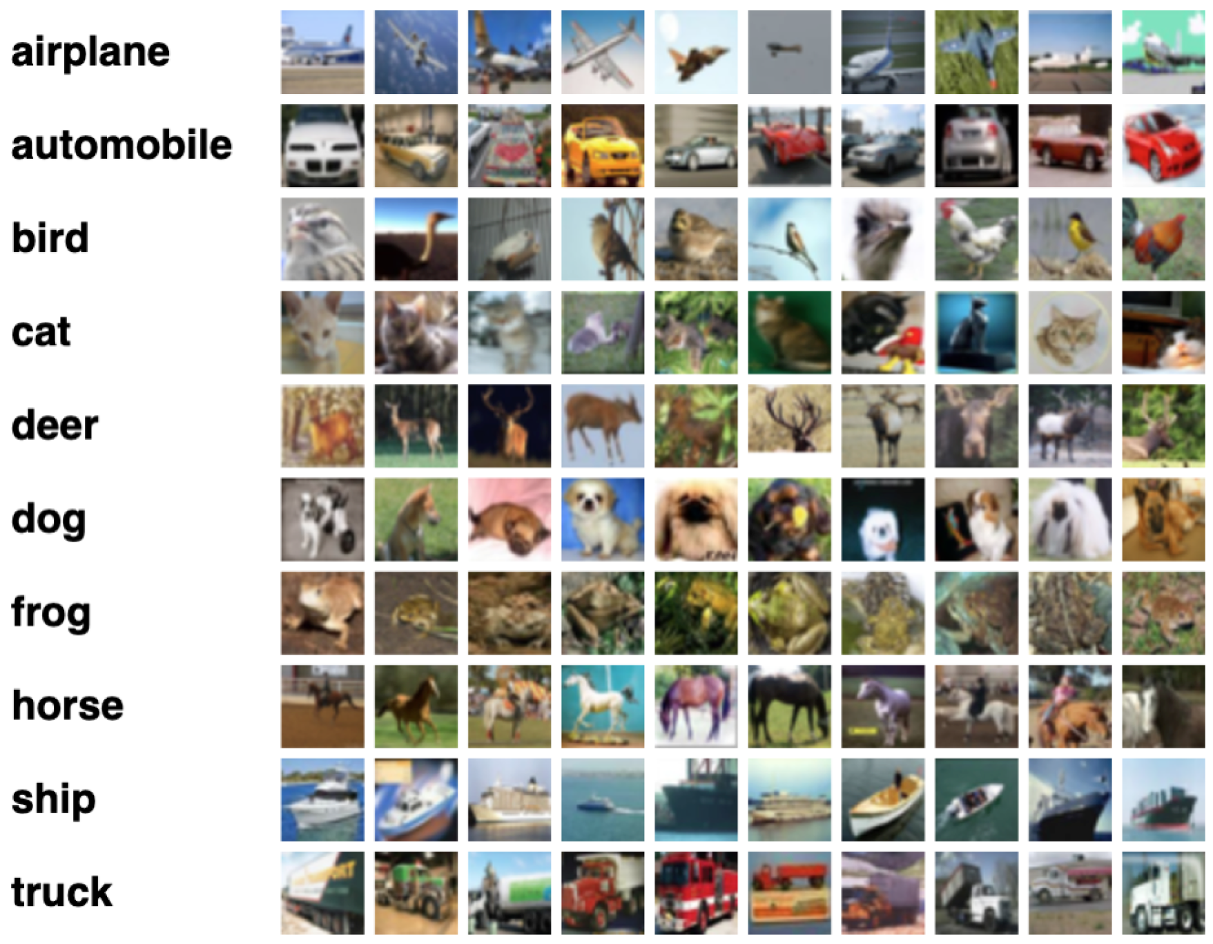
35] dataset is one of the most popular public datasets in current neural network architecture search work. CIFAR-10 is a small-scale image classification dataset proposed by Alex in 2009. As shown in Figure 1, there are 10 categories of data, namely aircraft, automobile, bird, cat, deer, dog, frog, horse, ship, and truck. Each category has 6000 images, each of which is a 32 × 32 sized RGB image. The entire CIFAR-10 dataset consists of 60,000 images, among these images, 50,000 images were classified for training and 10,000 images for testing.
2. CIFAR-100 Dataset.
As shown in Figure 2, the CIFAR-100 [
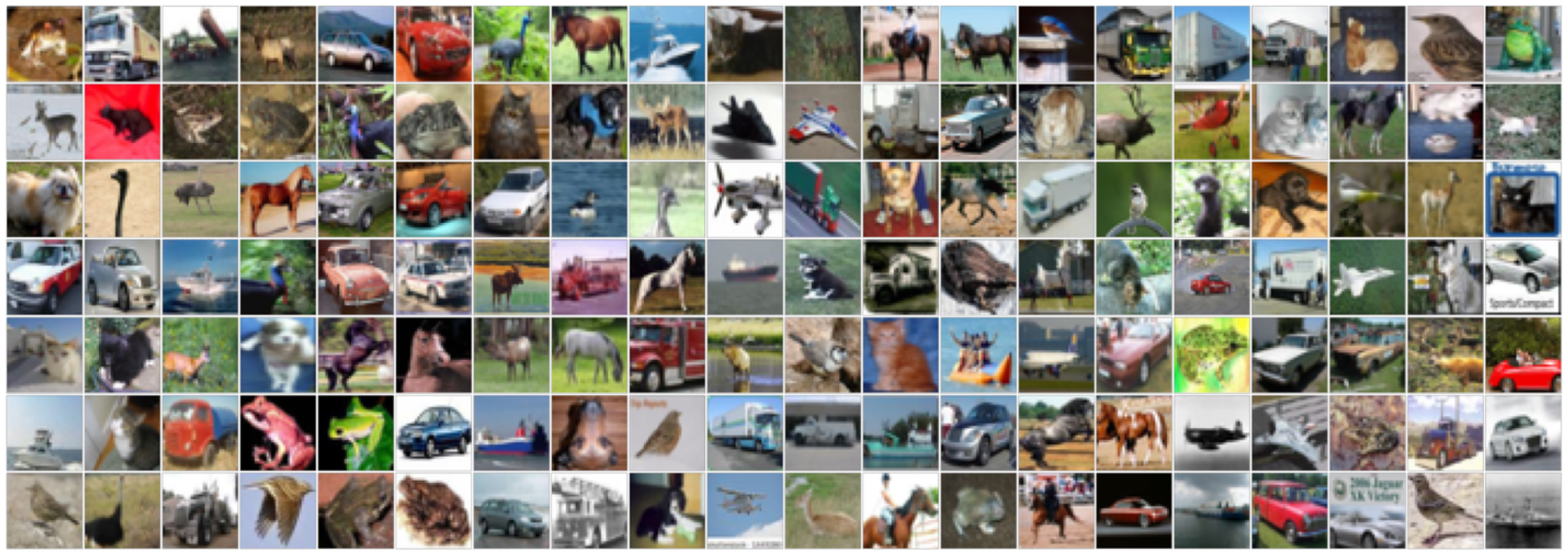
35] dataset is similar to the CIFAR-10 dataset, except that it has 100 classes. The 100 categories in CIFAR-100 are divided into 20 major categories. Each image comes with a “fine” label (the class it belongs to) and a “rough” label (the large class it belongs to).
During the experiment, the training set of CIFAR-10 and CIFAR-100 is randomly divided into two groups: one group will be used to update weight parameters while the other will serve as a validation set for updating schema parameters. This division is conducted for each category within the samples of the training set.
3. ImageNET Dataset.
ImageNet [
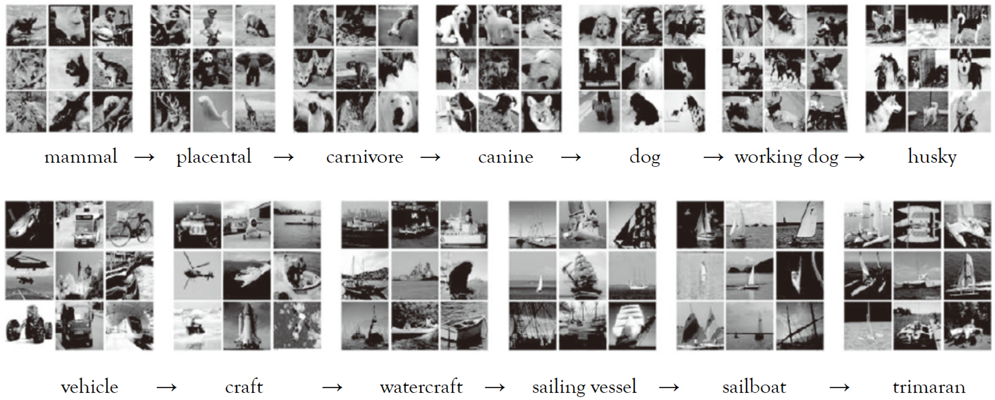
36] is an image dataset organized according to a WordNet hierarchy, where each node in the hierarchy is described by hundreds or thousands of images. The examples of the ImageNet dataset are shown in Figure 3. At present, there is an average of over 500 images per node, with a total number of images exceeding 10 million and a total of 1000 types of recognition. Compared to the CIFAR-10 and CIFAR-100 datasets, the ImageNet dataset has a larger number of images, higher resolution, more categories, and more irrelevant noise and changes in the images. Therefore, the recognition difficulty far exceeds that of CIFAR-10 and CIFAR-100.

3.1.2. Algorithm Settings

  • When optimizing neural network weight parameters through the gradient descent method, the optimization of shallower parameters relies on layer-by-layer back-propagation starting from the output layer, while the optimization of deeper parameters also relies on the feature data corresponding to the output values of shallower layers. Once subnetworks with different structures are obtained through training in this way, it is difficult to maintain the dependency relationship between shallow and deep layers, which can easily lead to significant deviations. During the training process using evolutionary algorithms, each weight parameter within the neural network holds a unique and independent position. This allows for individualized training and optimization of each parameter up to a certain extent. Then, different subnetworks can obtain better evaluation results when obtaining parameters from the super-network. Therefore, when conducting experiments in the DARTS search space, the improved evolutionary strategy in Section 2.3 was chosen to optimize the network weight parameters.
  • Each epoch is trained using a random small batch of samples [37], which reduces the computational complexity of each epoch while maintaining the training effect. At the same time, the algorithm can break through the sample data size limit and can be extended to large data volumes for calculation.

3.1.3. Search Space

1. DARTS search space.
The DARTS algorithm, serving as a fundamental neural network architecture search approach based on gradient descent, encompasses a substantial quantity of nodes and operation types within the building block (unit). The resulting network structure is achieved by stacking two structural units, thus leading to a high architectural complexity. Consequently, the DARTS search space has the potential to produce network models with superior performance. Currently, the majority of gradient-based methods undergo performance evaluation within the DARTS search space and are subsequently compared with other algorithms.
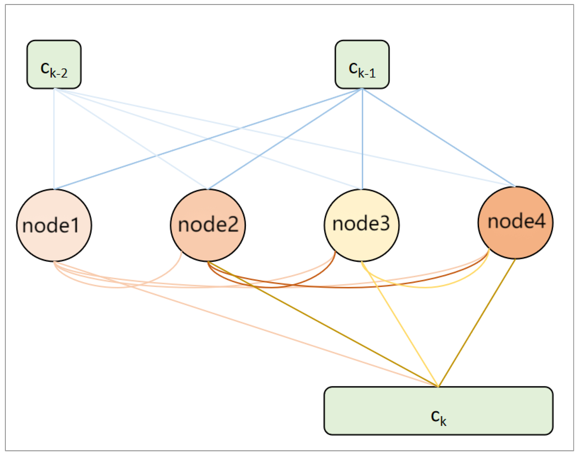
The unit structure of the DARTS search space shown in Figure 4, c k 2 , c k 1 , c k represents the outputs of units k 2 , k 1 , and k, respectively. In the k-th unit, there are four nodes between the outputs of the first two units and the output of the k-th unit. Each edge represents a candidate operation, with eight types of operations including extended separable convolutions of 3 × 3 and 5 × 5 , deep separable convolutions of 3 × 3 and 5 × 5 , average pooling of 3 × 3 , maximum pooling of 3 × 3 , identity operation, and zero operation. Zero operation indicates that there is no connection between two nodes, while identity operation indicates that the data from the previous node is directly transferred to the next node.
The entire network structure is composed of eight units, which are divided into standard units and down-sampling units. In the down-sampling unit, the first two nodes are connected to other nodes through pooling operations. The network consists of six standard units and two down-sampling units, which are located at one-third and two-thirds of the entire network.
2. NAS-Bench-201 Search space.
In current research, a growing number of NAS algorithms have been proposed. Despite their theoretical groundwork, many aspects of these algorithms display significant differences, including distinct search spaces, training strategies for architecture evaluation, and methods used to split validation sets. These differences lead to considerable challenges when comparing the performance of various NAS algorithms. As a result, researchers devote substantial computational resources to traverse and evaluate the performance of different search spaces and neural network structures, as well as their architectures within the designed network structure search space and producing datasets. Subsequent experiments on the NAS-Bench-201 search space [34] can obtain evaluation results through tabular queries without the need for retraining.
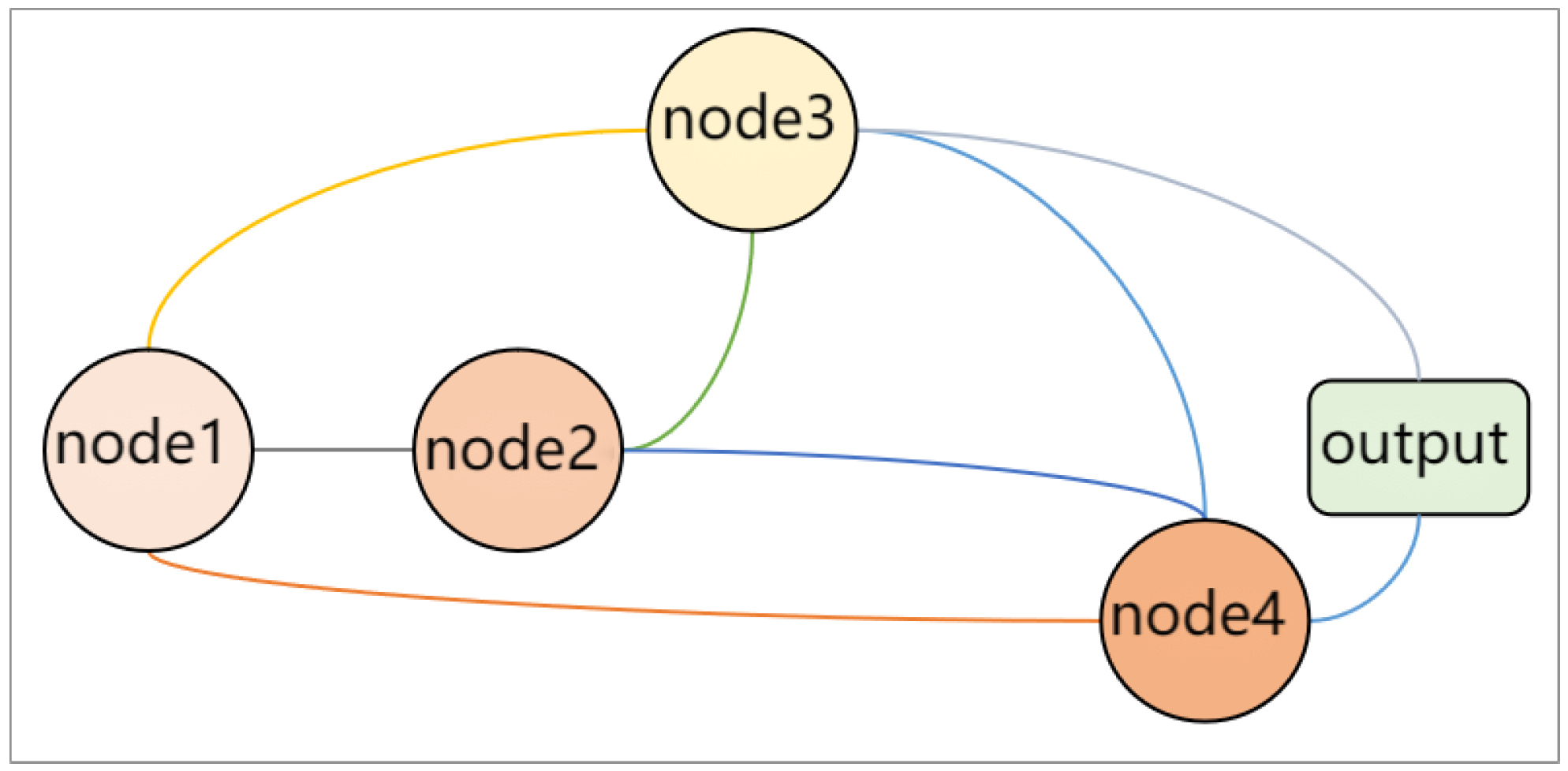
The structural units used in NAS-Bench-201 are shown in Figure 5. Each structural unit contains four nodes and five operation types ( 1 × 1 convolution, 3 × 3 convolution, 3 × 3 average pooling, identity operation, zero operation), totaling 5 6 = 15,625 types of unit structures.

3.1.4. Ablation Experiment

We first conducted ablation experiments on the NAS-Bench-201 search space to investigate the impact of parameters T , K , γ , γ α on the performance of NDARTS and determine the optimal experimental parameters. The ablation experiment used CIFAR-10 as the training dataset, and a pre-trained model was used to reduce computational complexity. The effects of different parameters were analyzed through 30 epochs of results.
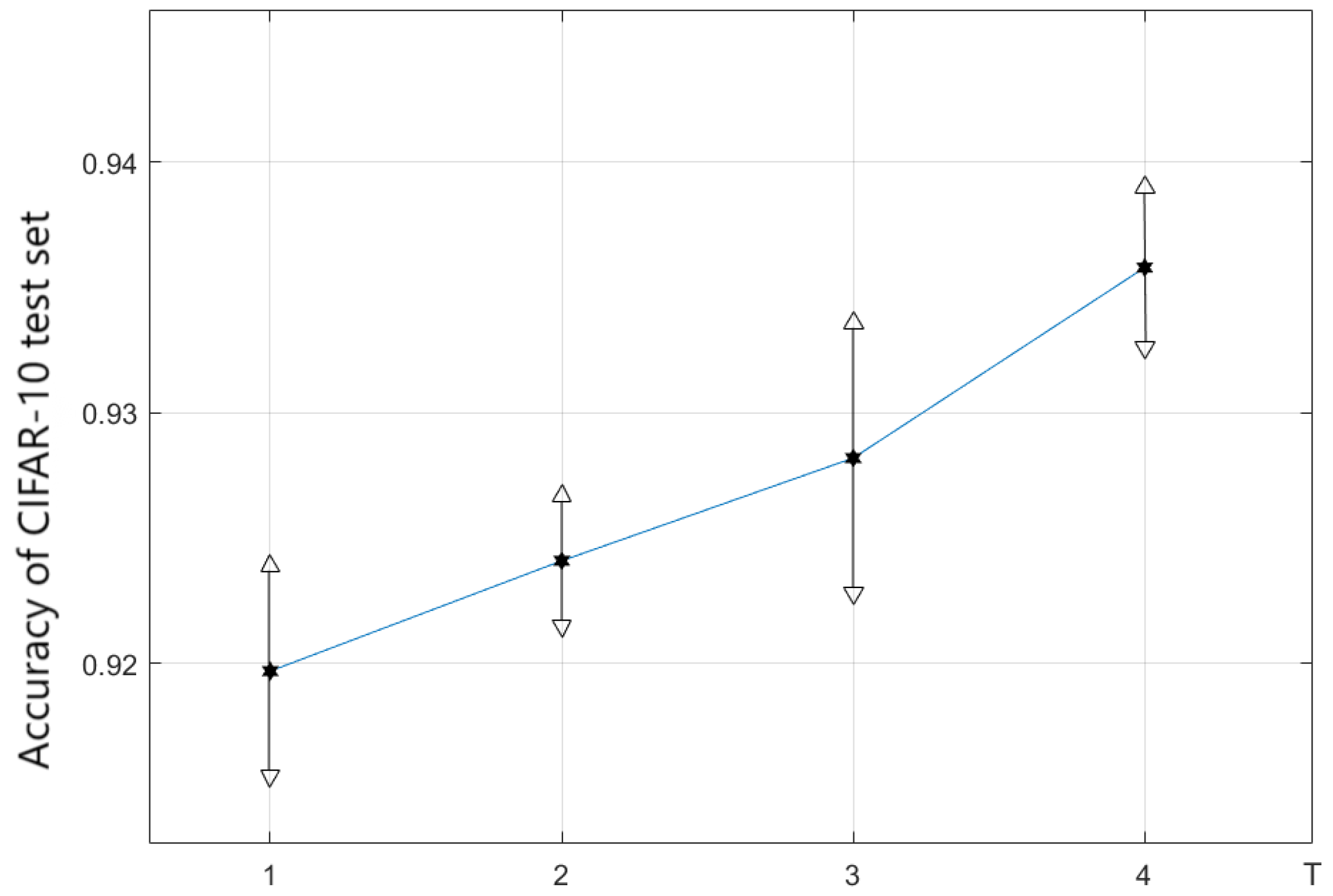
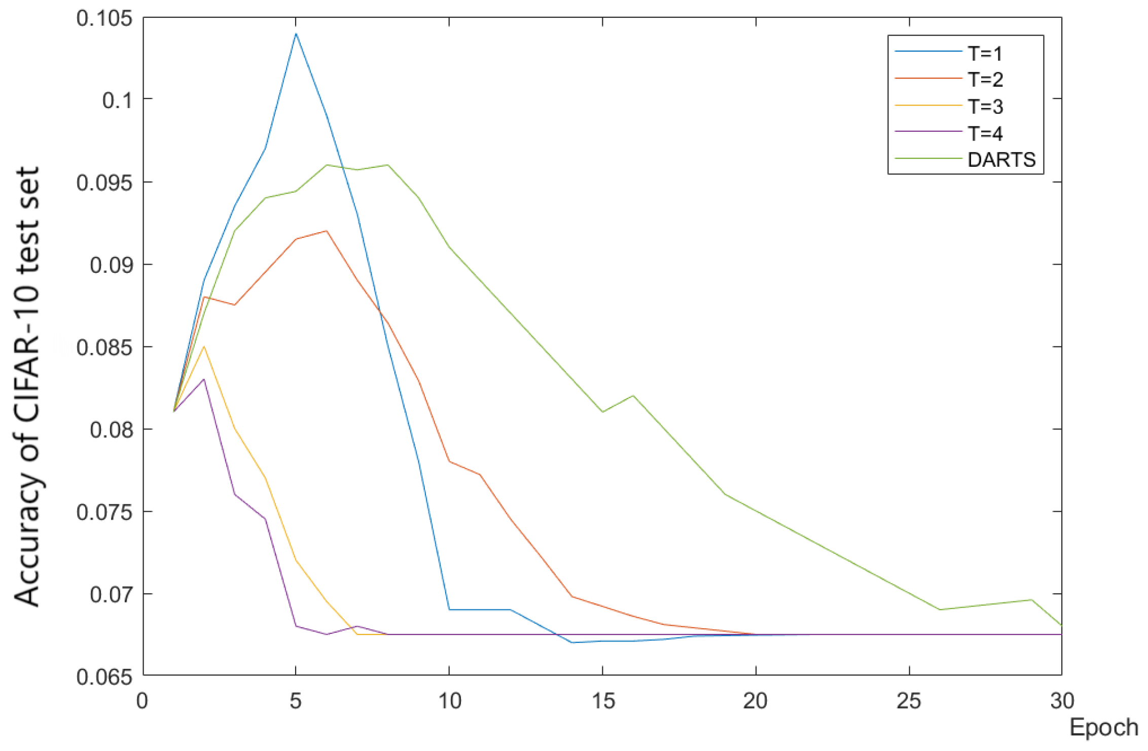
1. T.
Parameter T is the number of steps for updating the weight parameter ω during the update interval of the architecture parameter α . In theory, the larger the T, the more steps the ω updates during each time α is updating, and the ω is closer to the optimal value ω * . The better the performance of ω , the better the performance of the super-network when evaluating the architecture, and the more accurate the evaluation results of the subnetwork architecture, which helps the algorithm achieve a more approximate super-gradient estimation. However, the computational cost of the algorithm also increases with an increase in T. According to the experimental results, T = 4 achieved a good balance between computational cost and model performance.
The experimental results indicate that as T increases, the performance of the algorithm gradually improves. When T = 1 , both NDARTS and DARTS only optimize the weight parameter ω once within the update interval of the architecture parameter α , with the only difference being that NDARTS uses α L 2 ( ω ξ ω L 1 ( ω ( α ) , α ) ) , while DARTS uses α L 2 ( ω ( α ) , α ) to update the parameter α .
The experimental results are shown in Figure 6 and Figure 7; it can be seen that NDARTS at T = 1 can search for a better framework with faster convergence speed and higher stability compared to the benchmark algorithm DARTS. When T increased from 1 to 4, the algorithm achieved better convergence speed and stability.
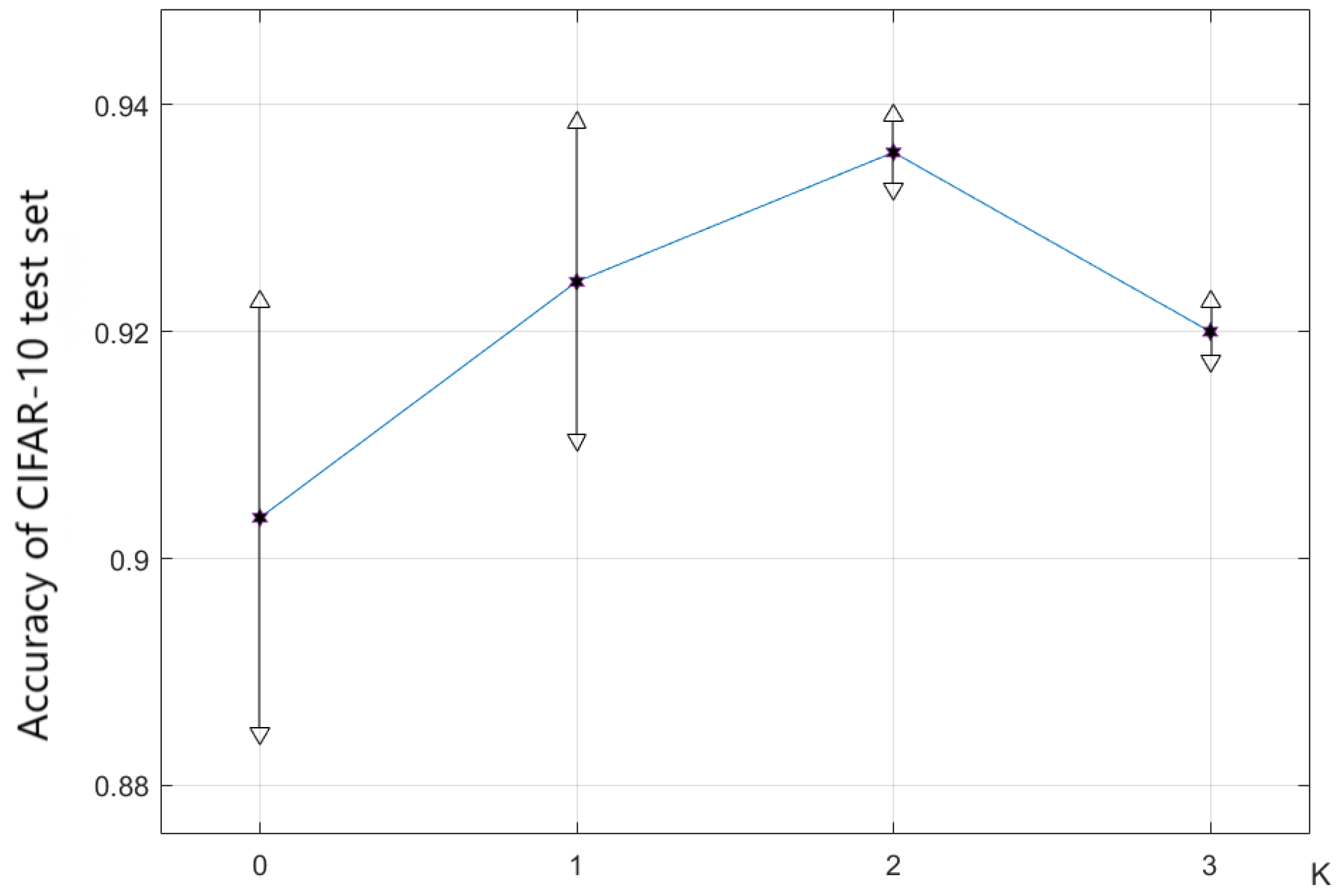
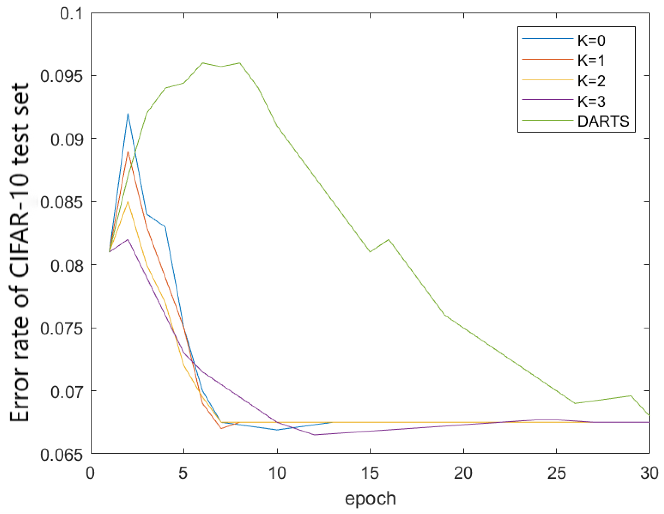
2. K.
The parameter K represents the number of truncated approximations utilized in the optimization formula. The larger the K, the smaller the error γ L 2 ω j = K + 1 ( I γ 2 L 1 ω ω ) j 2 L 1 ω ω is, which is between the approximate gradient value α L 2 and the true gradient α L 2 . Therefore, in theory, as K increases, the performance of the neural network should also increase.
From the experimental results in Figure 8 and Figure 9, it can be seen that when K increases from 0 to 2, the accuracy of the model searched by the algorithm increases from 90.36 % to 93.58 % , and the stability of the search increases with an increase in K. Another conclusion is that K = 2 is already large enough, so that when K 3 is used, the algorithm performance cannot be further improved. But when K 2 continues to increase, the stability of the algorithm still shows an increasing trend, and when K = 2 , the algorithm has already reached a good stability.
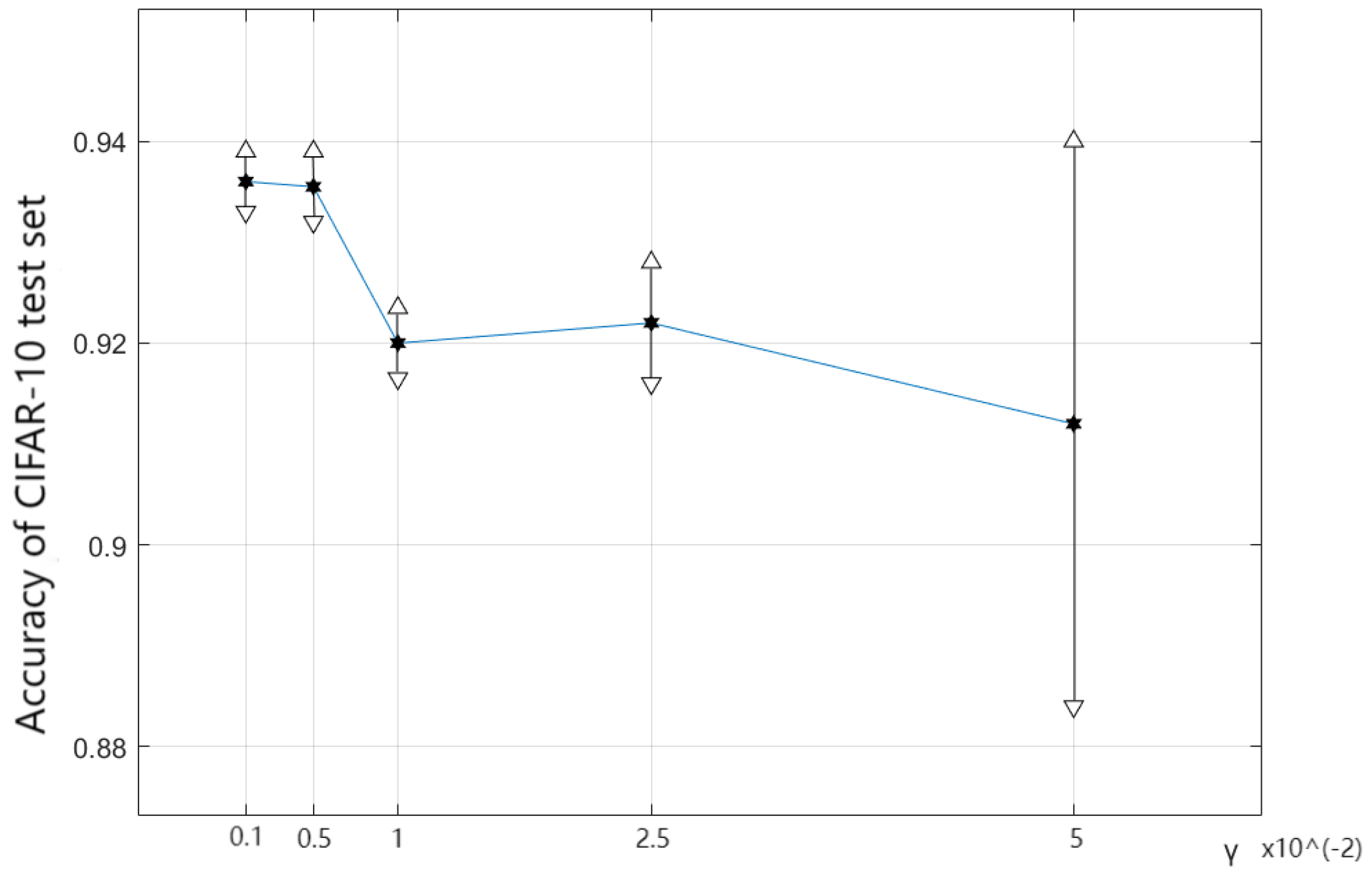
3. γ and γ α .
The calculation of NDARTS is based on the approximation of L 2 using the Neumann series, with the potential condition that the learning rate γ should be small enough to make | | I γ 2 L 1 ω ω | | < 1 .
As shown in Figure 10, when γ = 0.001 and 0.005 , the algorithm can maintain a good accuracy and stability. When γ = 0.01 , the algorithm performance slightly decreases, and the accuracy decreases from 93.58 % to 92.02 % , indicating good stability. When γ = 0.025 , the accuracy of the algorithm is 92.17 % , but the stability of the model begins to decrease. When γ = 0.05 , the performance of the algorithm decreases again, with a model accuracy of 91.22 % , and the stability of the algorithm is significantly reduced.
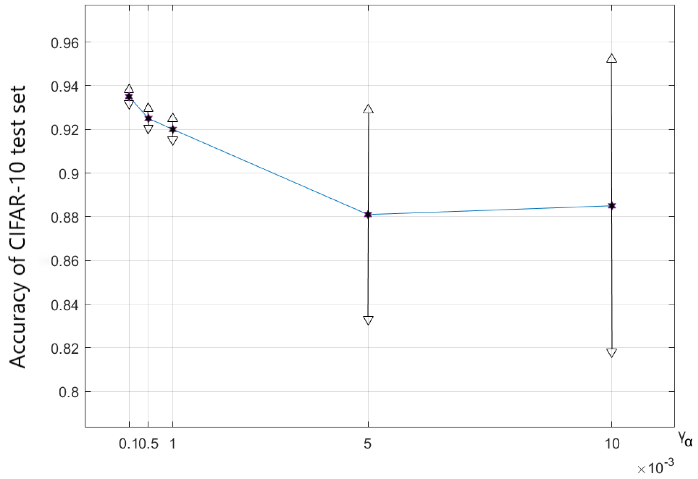
In NDARTS, the parameter γ α should take a small value to make the coefficient ( 1 P ) L α L 2 2 γ α m ( 1 + D ) > 0 . As shown in Figure 11, when γ α increases from 0.0001 to 0.001 . The performance of the algorithm decreases from 93.58 % to 92.04 % , with relatively small stability changes. But when γ α increases from 0.001 to 0.005 and 0.01 , the performance and stability of the algorithm are significantly reduced.
In summary, NDARTS has strong sensitivity to parameters γ and γ α , chooses smaller γ , and γ α can help maintain the performance and stability of NDARTS. The dependence of NDARTS on parameters T and K is relatively small. Larger T and K can improve the convergence speed and performance of the algorithm, but also increase computational costs. Choosing the appropriate T and K can reduce computational costs while maintaining good performance of the NDARTS.

3.1.5. Performance Experiment

The ablation experiment determined the optimal parameters of NDARTS. Subsequently, we tested the performance of NDARTS in the DARTS search space and NAS-Bench-201 search space under the optimal parameters and compared it with other algorithms at similar model scales. Because of the limited computational resources, we mainly tested gradient-based algorithms, and other results are compared using the results of the original paper, marked with * in Tables. The algorithm tested in this article will provide a reference for the accuracy of the validation set as an additional condition, and the program list will be provided in Appendix A.
DARTS search space.
Comparing the results of the NDARTS algorithm in the DARTS search space with other NAS algorithms, the results on the CIFAR-10, CIFAR-100, and ImageNet datasets are shown in Table 1, Table 2 and Table 3, respectively.
Overall, compared with other types of methods, such as random search and RL, NDARTS has a significant increase in performance. And methods based on random search, RL, and EA have longer computational time, and NDARTS can achieve better performance in a short period. Although the PNAS [9] algorithm based on sequential models also requires smaller computational resources, the cost is to reduce the accuracy of the model.
Compared with the baseline algorithm DARTS, which is based on gradient descent, NDARTS improves the performance of the algorithm while reducing a certain computational cost. FairDARTS [38] relaxes the choice of operations to be collaborative, where the authors let each operation have an equal opportunity to develop its strength, but our algorithm performed better than FairDARTS. PDARTS [24] searches for neural network architecture progressively, achieving good accuracy at a higher computational cost, while NDARTS achieves better performance at a lower computational cost. PC-DARTS [25] reduces computational costs by sampling channels, and can quickly obtain models with better performance. Although NDARTS has a slightly slower speed than PC-DARTS, it has better performance. In the DARTS search space, NDARTS achieved optimal performance on all three datasets.
Table 1. Results of NDARTS (based on DARTS search space) and other NAS algorithms on the CIFAR-10 dataset.
AlgorithmVal Error (%)Test Error (%)Param (m)Search SpaceSearch Method
RandomNAS [39] *——2.654.3DARTSRandom search
AmoebaNet *——3.345.1NASNetEA
NASNet *——2.655.3NASNetRL
PNAS *——3.415.1DARTSSequential
ENAS *——2.894.6NASNetRL
GDAS * [40]——2.933.4DARTSGradient
SETN * [41]——2.694.6DARTSGradient
FairDARTS [38]3.822.542.83DARTSGradient
PDARTS3.992.503.4DARTSGradient
PC-DARTS3.882.573.6DARTSGradient
DARTS4.382.763.4DARTSGradient
NDARTS3.982.373.8DARTSGradient
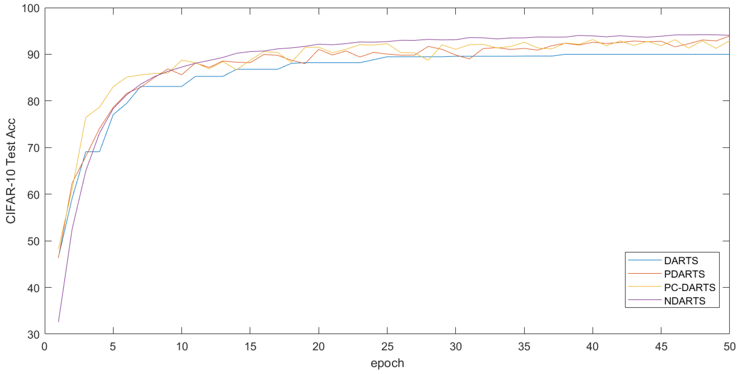
The results on the CIFAR-10 dataset are shown in Table 1. This article ran some algorithms and displayed the accuracy of the test set in Figure 12 (truncated to 50 epochs due to different algorithm settings). It can be seen that the performance of models searched based on gradient methods is generally better than those searched by algorithms based on random search, RL, and other methods. Among gradient-based methods, NDARTS achieved the best performance on the CIFAR-10 dataset, with a test set error of only 2.37 % , which is superior to other gradient methods such as FairDARTS, PDARTS, PC-DARTS, and DARTS with 2.54 % , 2.50 % , 2.57 % , and 2.76 % . And, it can be seen from the iteration curve in Figure 12 that even if the initial state is worse, NDARTS can still quickly optimize to a better model.
Table 2. Results of NDARTS (based on DARTS search space) and other NAS algorithms on the CIFAR-100 dataset.
AlgorithmVal Error (%)Test Error (%)Param (m)Search SpaceSearch Method
RandomNAS *——17.634.3DARTSRandom
NASNet-A *——17.813.3NASNetRL
PNAS *——17.633.2DARTSSequential
GDAS *——18.383.4DARTSGradient
SETN *——17.254.6DARTSGradient
PDARTS19.9717.43.4DARTSGradient
PC-DARTS20.2517.113.6DARTSGradient
DARTS21.4217.543.4DARTSGradient
NDARTS16.1716.023.8DARTSGradient
Table 3. Results of NDARTS (based on DARTS search space) and other NAS algorithms on the ImageNet dataset.
AlgorithmTop1 Test Error (%)Top5 Test Error (%)Param (m)Search SpaceSearch Method
RandomNAS *27.1——4.3DARTSRandom
AmoebaNet-A *25.58.05.1NASNetEA
NASNet-A *26.08.43.3NASNetRL
PNAS *25.88.13.2DARTSSequential
GDAS *26.08.53.4DARTSGradient
SETN *25.78.04.6DARTSGradient
SharpDARTS [42]25.17.84.9DARTSGradient
PDARTS *24.47.43.4DARTSGradient
PC-DARTS *25.17.83.6DARTSGradient
DARTS26.98.73.4DARTSGradient
NDARTS24.37.33.8DARTSGradient
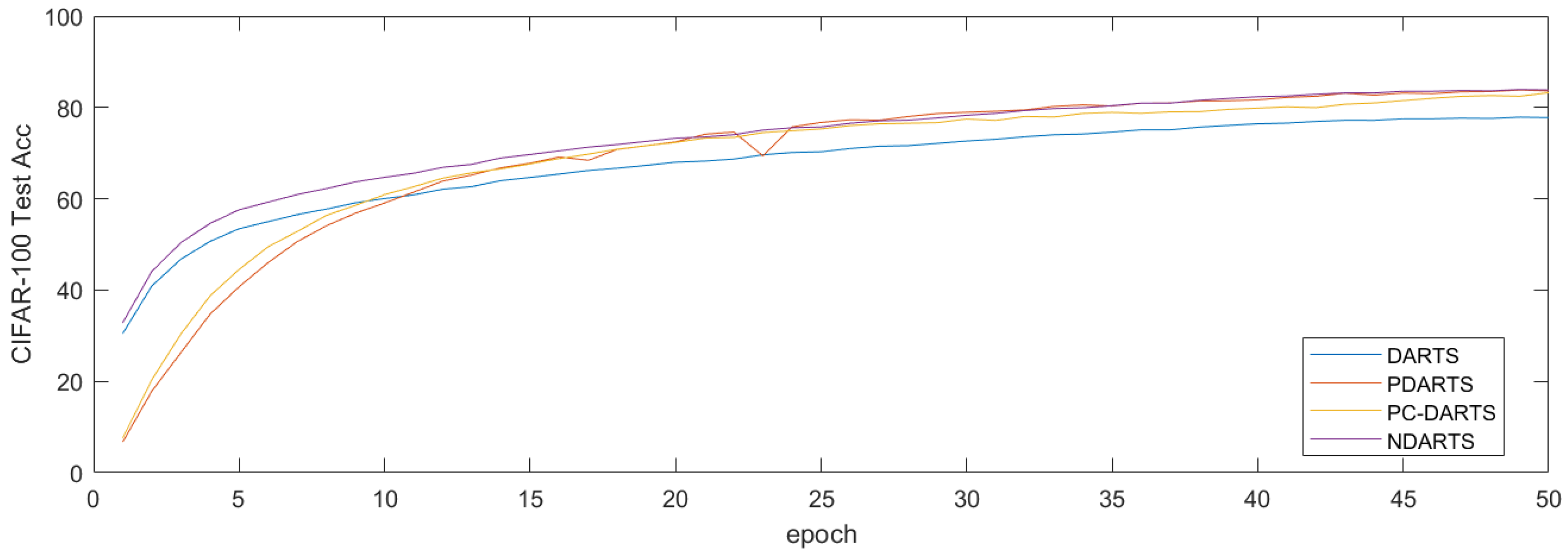
The results on the CIFAR-100 dataset are shown in Table 2, and the 50 epoch iteration curves of some algorithms are plotted in Figure 13. The results showed that NDARTS outperforms other gradient-methods with an error of 16.02 % , while the performance of GDAS on the CIFAR-100 dataset drops to a Test Error of 18.38 % . In addition, gradient-based methods are generally superior to other algorithms based on random search, RL, and other methods. From the iteration curve, it can be seen that NDARTS, PDARTS, and PC-DARTS have similar search speeds, they have faster search speeds and better performance than DARTS.
The results on ImageNet are shown in Table 3. When extended to big data, the gradient method can no longer maintain its superiority over other methods in performance, but the NDARTS algorithm still achieved optimal performance with 24.3 % and 7.3 % TOP1 and TOP5 Test ERROR, respectively.
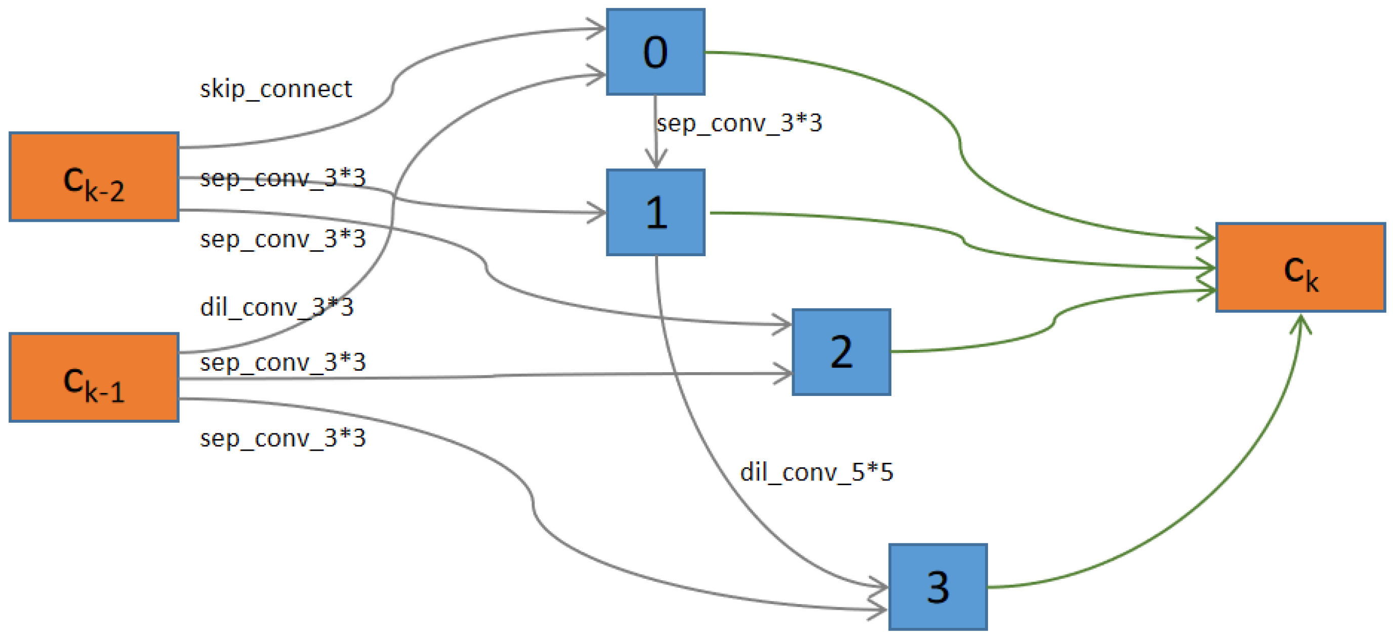
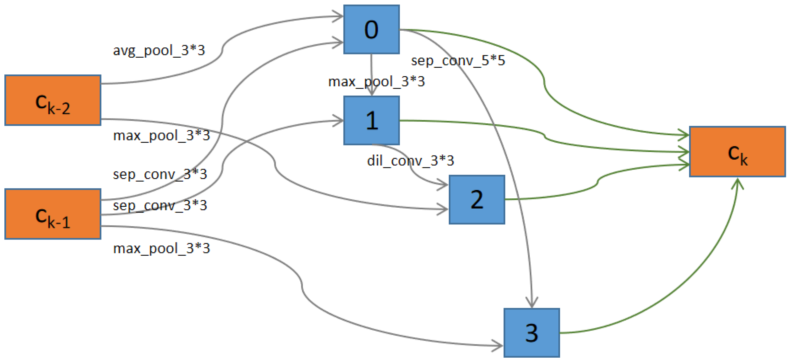
Figure 14 and Figure 15 showed the structures of Normal Cells and Reduction Cells searched by NDARTS in the DARTS search space. As we can see, there are four nodes between the outputs of units k 1 , k 2 and the output of unit k. There are some operations on each edge. There are also some pooling operations in the Reduction cell, which can reduce the feature map height and width by a factor of two.
NAS-BENCH-201 search space.
The performance of the NDARTS algorithm and other NAS algorithms was tested in the NAS-Bench-201 search space. The results on CIFAR-10, CIFAR-100, and ImageNet datasets are shown in Table 4, Table 5 and Table 6, respectively. Among them, each algorithm searches for the optimal structural unit on the CIFAR-10 dataset and evaluates its performance on the CIFAR-100 and ImageNet datasets.
Due to the simpler unit search space of NAS-Bench-201 than the DARTS search space, the algorithm performance generally decreases in the NAS-Bench-201 search space. Overall, due to the omission of a large amount of training and evaluation calculations in the NAS-Bench-201 search space, the RL- and EA-based methods have shown good performance. The architecture search algorithm using random search as the baseline still exhibits certain search capabilities in the NAS-Bench-201 search space. The gradient-based method exhibits adaptive differences in the NAS-Bench-201 search space, while the GDAS algorithm, which performs poorly in the DARTS search space, exhibits good performance in the NAS-Bench-201 search space. The model searched by the NDARTS algorithm achieves optimal performance or approaches optimal performance on the three datasets.
The results of the CIFAR-10 dataset are shown in Table 4, and the results of 50 epochs intercepted using gradient-based methods are plotted in Figure 16. It can be seen that the methods based on RL and EA have shown good performance in the NAS-Bench-201 search space. DARTS experienced severe performance degradation, while GDAS, which performed poorly in the DARTS search space, maintained good model performance, while NDARTS had a slightly better test set accuracy of 93.67 % than the 93.49 % of GDAS. From Figure 16, it can be seen that DARTS is difficult to search for good architectures in the NAS-Bench-201 search space. The SETN [30] algorithm with good initial model performance has an unstable search process, while the GDAS and NDARTS algorithms can effectively search for better architectures.
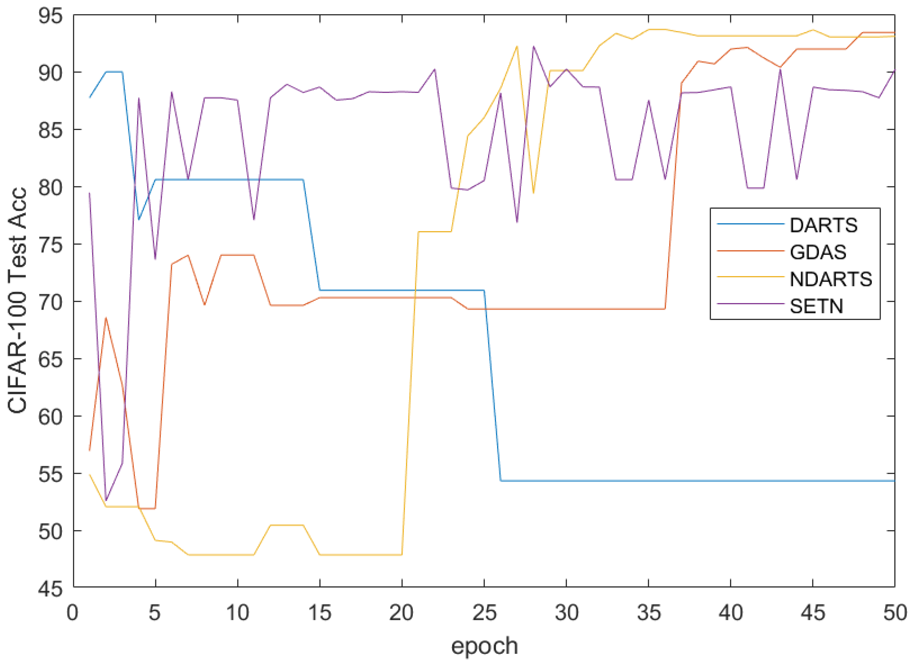
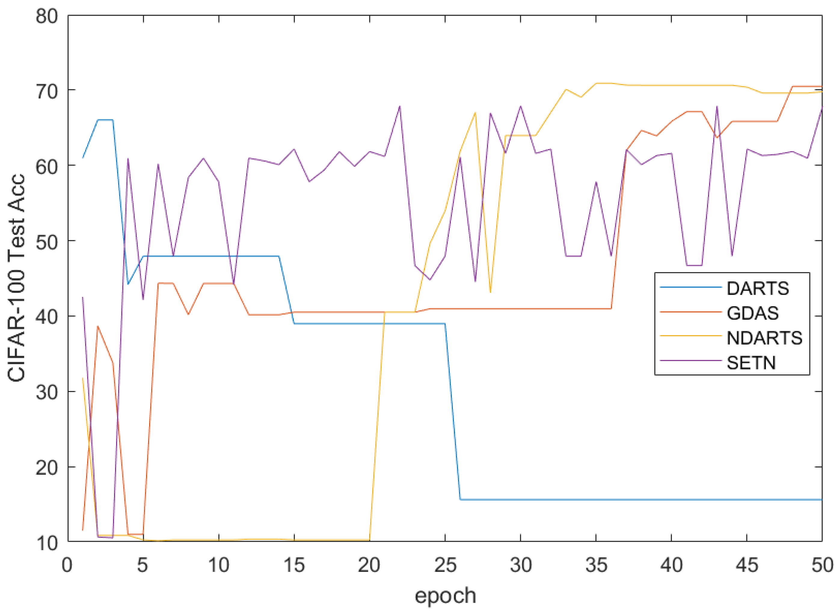
The results of the CIFAR-100 dataset are shown in Table 5, and the results of intercepting 50 epochs using gradient-based methods are plotted in Figure 17. It can be seen that on the CIFAR-100 dataset, NDARTS performed with an accuracy of 70.91 % , almost approaching the optimal performance of 71.00 % achieved by EA, while GDAS also maintained a good performance of 70.28 % . However, DARTS and ENAS [14] methods even have poorer performance compared to methods based on random search. In Figure 17, when comparing the results of the gradient method, GDAS and NDARTS have similar performance and are superior to DARTS and SETN.
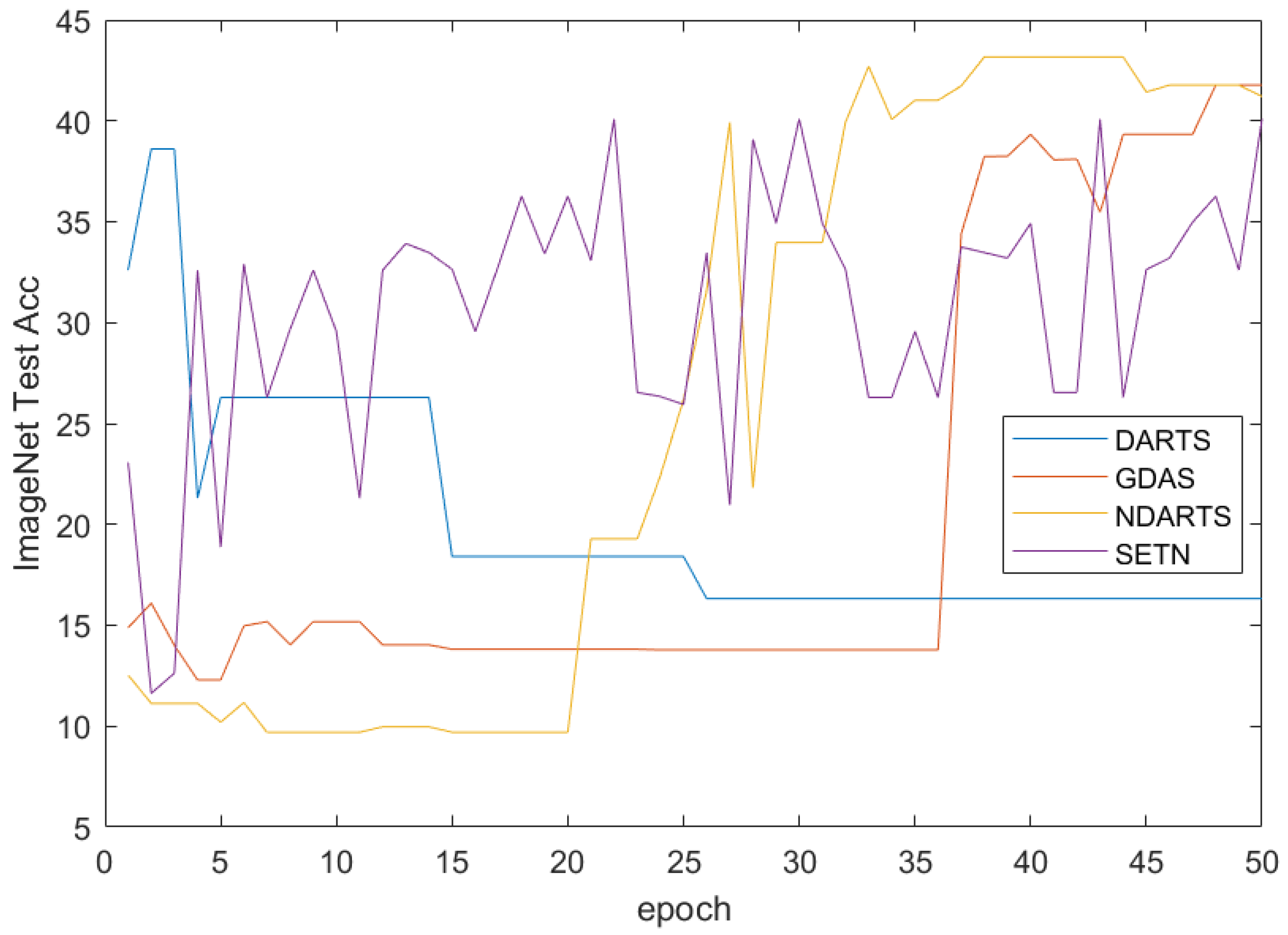
The results of the ImageNet dataset are shown in Table 6, and the results of intercepting 50 epochs using gradient-based methods are plotted in Figure 18. It can be seen that on the ImageNet dataset, the evolutionary algorithm-based method achieved the best performance with an accuracy of 44.23 % , while the reinforcement learning-based method also achieved an accuracy of 42.23 % . In gradient-based methods, GDAS achieves the best accuracy with 43.10 % , while NDARTS performs slightly worse with 41.02 % . The methods based on evolutionary algorithms and reinforcement learning can achieve good performance with the support of a large amount of computing resources. The NAS-Bench-201 search space uses a table query form for performance evaluation, especially on large datasets such as ImageNet, which saves a lot of computation. Therefore, the methods based on EA and RL have shown good performance on the NAS-Bench-201 search space and ImageNet dataset. The gradient-based methods has significant performance differences in the NAS-Bench-201 search space and ImageNet dataset. Specifically, as shown in Figure 18, GDAS and NDARTS perform better than SETN and DARTS. Although GDAS and NDARTS have poor initial states, they can still quickly optimize to better models, while SETN has a slower search speed and unstable search process, DARTS makes it difficult to search for better models in the NAS-Bench-201 search space.
To compare the performance of NDARTS and GDAS in detail, the results of all epochs on the three datasets were plotted as shown in Figure 19. It can be seen that NDARTS has a faster search speed than GDAS. When approaching stability, NDARTS and GDAS search for the same model for a long time but ultimately stop at different architectures. At this time, NDARTS has better performance than GDAS on CIFAR-10 and CIFAR-100 datasets, but slightly worse performance on ImageNet datasets.
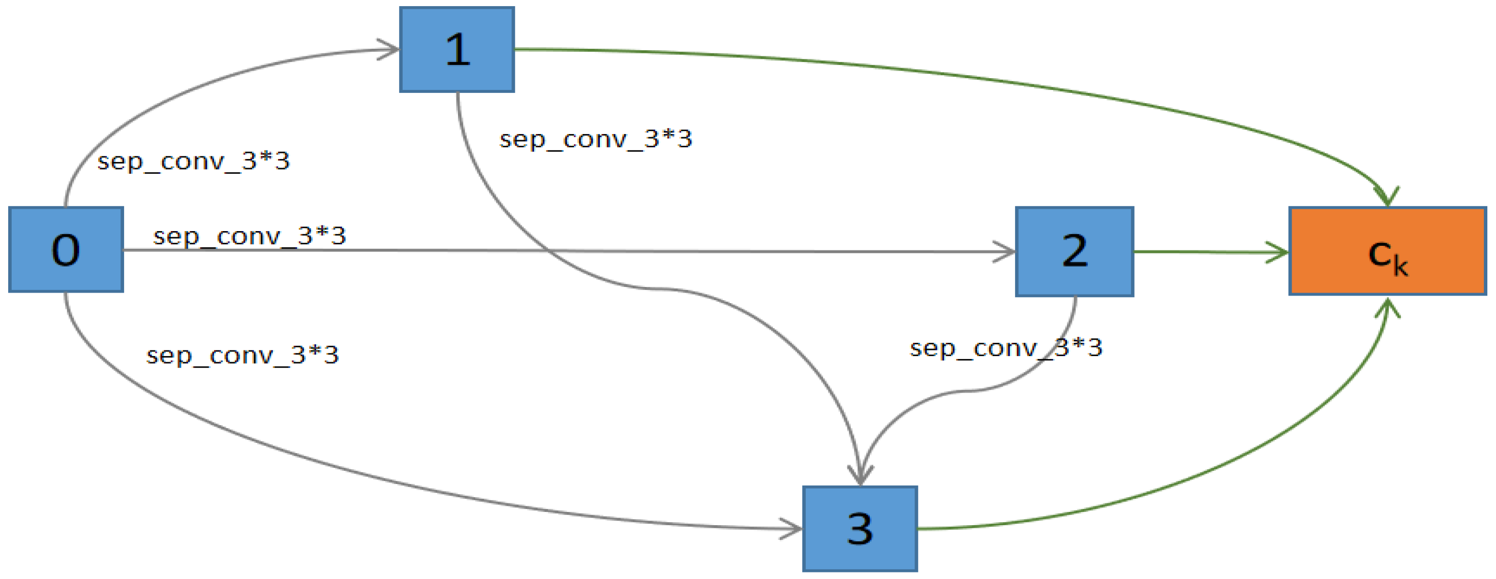
The model cell structure searched by the NDARTS algorithm is shown in Figure 20. As we can see, there is just one kind of cell in the NAS-Bench-201 search space. And there are just three intermediate nodes between the input and output. Finally, we can obtain the network by stacking the searched cell.

3.2. Experiment Results

DARTS search space is the most fundamental search space for gradient-based neural network architecture search algorithms, with two cell types and multiple nodes, as well as multiple operation types. When compared with other algorithms in the DARTS search space, NDARTS achieved better performance than mainstream NAS algorithms on CIFAR-10, CIFAR-100, and ImageNet datasets.
Compared to the DARTS search space, the NAS-Bench-201 search space has fewer unit types, fewer number of nodes in the unit, and fewer operation types. Although the performance of the searched model is relatively low, it can compare the performance of different NAS algorithms under a fair evaluation strategies conditions. When compared with other algorithms in the NAS-Bench-201 search space, the NDARTS algorithm achieved optimal performance on the CIFAR-10 dataset, outperforming than other gradient based methods and approaching optimal evolutionary algorithm performance on the CIFAR-100 dataset. The results on the ImageNet dataset also approached the performance of the optimal evolutionary algorithm.
In summary, NDARTS maintains a small computational cost at the same time improving its performance compared to mainstream NAS algorithms. It exhibits good adaptability in different structural search spaces and is a highly competitive neural network architecture search algorithm.

4. Conclusions

By approximating the iterative update formula of the DARTS algorithm based on Neumann series, it can be proven that the approximate iterative method is still convergent while reducing computational complexity. When optimizing weight parameters, choose an evolutionary strategy to avoid problems during the training process caused by gradient methods. Simulation experiments on CIFAR-10, CIFAR-100, and ImageNet datasets have shown that NDARTS is a highly competitive neural network architecture search algorithm.
Although our gradient approximation is more accurate and performs better than the DARTS algorithm. However, our algorithm still has some limitations, our algorithm has large gap between the architecture depths in search and evaluation scenarios, and performance gaps between discrete subnetworks and hyper-networks, which need to improvement in the further.
The algorithm model for designing the search space in the article is based on unit structure stacking, but it has certain limitations. The main reason is that the network instances obtained from the search can only be applicable to a specific configuration, and the generalization ability for different configurations is weak. So, for different experimental data scenarios, we need to develop an NAS algorithm that can search high performance network architecture.

Author Contributions

Conceptualization, X.H. and Z.W.; writing—original draft preparation, X.H.; writing—review and editing, C.L.; supervision, G.L. All authors have read and agreed to the published version of the manuscript.

Funding

This research received no external funding.

Data Availability Statement

All the experimental datasets can be found in CIFAR-10, CIFAR-100: http://www.cs.toronto.edu/~kriz/cifar.html (accessed on 7 October 2023) and ImageNet http://image-net.org/ (accessed on 7 October 2023).

Conflicts of Interest

The authors declare no conflict of interest.

Abbreviations

The following abbreviations are used in this manuscript:
NASNeural Architecture Search
RLReinforcement
EAEvolutionary Algorithm
MDPIMultidisciplinary Digital Publishing Institute

Appendix A

Algorithms cited in this article:
DARTS: https://github.com/quark0/darts (accessed on 7 October 2023).
FairDARTS: https://github.com/xiaomi-automl/FairDARTS (accessed on 7 October 2023).
SharpDARTS: https://github.com/ahundt/sharpDARTS (accessed on 7 October 2023).
PDARTS: https://github.com/chenxin061/pdarts (accessed on 7 October 2023).
PC-DARTS: https://github.com/yuhuixu1993/PC-DARTS (accessed on 7 October 2023).
NAS-Bench-201 Search Space and Related Algorithms: https://github.com/D-X-Y/NATS-Bench (accessed on 7 October 2023).

References

  1. Wu, Y.; Schuster, M.; Chen, Z.; Le, Q.V.; Norouzi, M.; Macherey, W.; Krikun, M.; Cao, Y.; Gao, Q.; Macherey, K.; et al. Google’s Neural Machine Translation System: Bridging the Gap between Human and Machine Translation. arXiv 2016, arXiv:1609.08144. [Google Scholar]
  2. Chen, M.X.; Firat, O.; Bapna, A.; Johnson, M.; Macherey, W.; Foster, G.; Jones, L.; Parmar, N.; Schuster, M.; Chen, Z.; et al. The Best of Both Worlds: Combining Recent Advances in Neural Machine Translation. arXiv 2016, arXiv:1804.09849. [Google Scholar] [CrossRef]
  3. Simonyan, K.; Zisserman, A. Very Deep Convolutional Networks for Large-Scale Image Recognition. In Proceedings of the International Conference on Learning Representations.Computational and Biological Learning Society, San Diego, CA, USA, 7–9 May 2015. [Google Scholar]
  4. Howard, A.G.; Zhu, M.; Chen, B.; Kalenichenko, D.; Wang, W.; Weyand, T.; Andreetto, M.; Adam, H. MobileNets: Efficient Convolutional Neural Networks for Mobile Vision Applications. arXiv 2017, arXiv:1704.04861. [Google Scholar]
  5. Ren, S.; He, K.; Girshick, R.; Sun, J. Faster R-CNN: Towards Real-Time Object Detection with Region Proposal Networks. IEEE Trans. Pattern Anal. Mach. Intell. 2017, 39, 1137–1149. [Google Scholar] [CrossRef] [PubMed]
  6. Girshick, R.; Donahue, J.; Darrell, T.; Malik, J. Rich Feature Hierarchies for Accurate Object Detection and Semantic Segmentation Tech Report (v5). arXiv 2014, arXiv:1311.2524. [Google Scholar]
  7. He, K.; Zhang, X.; Ren, S.; Sun, J. Deep Residual Learning for Image Recognition. In Proceedings of the IEEE Conference on Computer Vision and Pattern Recognition, Las Vegas, NV, USA, 27–30 June 2016. [Google Scholar]
  8. Dong, X.; Huang, J.; Yang, Y.; Yan, S. More is Less: A More Complicated Network with Less Inference Complexity. In Proceedings of the IEEE Conference on Computer Vision and Pattern Recognition, Honolulu, HI, USA, 21–26 July 2017. [Google Scholar]
  9. Elsken, T.; Metzen, J.H.; Hutter, F. Neural architecture search: A survey. J. Mach. Learn. Res. 2019, 20, 1997–2017. [Google Scholar]
  10. Baker, B.; Gupta, O.; Naik, N.; Raskar, R. Designing Neural Network Architectures using Reinforcement Learning. arXiv 2016, arXiv:1611.02167. [Google Scholar]
  11. Ren, P.; Xiao, Y.; Chang, X.; Huang, P.Y.; Li, Z.; Chen, X.; Wang, X. A Comprehensive Survey of Neural Architecture Search: Challenges and Solutions. ACM Comput. Surv. 2022, 54, 1–34. [Google Scholar] [CrossRef]
  12. Zoph, B.; Vasudevan, V.; Shlens, J.; Le, Q.V. Learning Transferable Architectures for Scalable Image Recognition. arXiv 2017, arXiv:1707.07012. [Google Scholar]
  13. Enzo, L.A.; Eduardo, L.; Vasty, Z.; Claudia, R.; John, M. Neural Architecture Search with Reinforcement Learning. arXiv 2016, arXiv:1611.01578. [Google Scholar]
  14. Cai, H.; Chen, T.; Zhang, W.; Yu, Y.; Wang, J. Efficient Architecture Search by Network Transformation. arXiv 2017, arXiv:1707.04873. [Google Scholar] [CrossRef]
  15. Real, E.; Aggarwal, A.; Huang, Y.; Le, Q.V. Regularized Evolution for Image Classifier Architecture Search. Proc. Aaai Conf. Artif. Intell. 2018, 33, 4780–4789. [Google Scholar] [CrossRef]
  16. Liu, H.; Simonyan, K.; Vinyals, O.; Fernando, C.; Kavukcuoglu, K. Hierarchical Representations for Efficient Architecture Search.International Conference on Learning Representations. arXiv 2018, arXiv:1711.00436. [Google Scholar]
  17. Real, E.; Moore, S.; Selle, A.; Saxena, S.; Suematsu, Y.L.; Tan, J.; Le, Q.V.; Kurakin, A. Large-Scale Evolution of Image Classifiers. arXiv 2017, arXiv:1703.01041. [Google Scholar]
  18. Stanley, K.O.; Miikkulainen, R. Evolving neural networks through augmenting topologies. Evol. Comput. 2002, 10, 99–127. [Google Scholar] [CrossRef] [PubMed]
  19. Xie, L.; Yuille, A. Genetic CNN. In Proceedings of the 2017 IEEE International Conference on Computer Vision (ICCV), Venice, Italy, 22–29 October 2017. [Google Scholar]
  20. Liu, C.; Zoph, B.; Neumann, M.; Shlens, J.; Wei, H.; Li, L.-J.; Li, F.-F.; Yuille, A.; Huang, J.; Murphy, K. Progressive Neural Architecture Search. arXiv 2017, arXiv:1712.00559. [Google Scholar]
  21. Kandasamy, K.; Neiswanger, W.; Schneider, J.; Póczos, B.; Xing, E.P. Neural Architecture Search with Bayesian Optimisation and Optimal Transport. arXiv 2018, arXiv:1802.07191. [Google Scholar]
  22. Negrinho, R.; Gordon, G. DeepArchitect: Automatically Designing and Training Deep Architectures. arXiv 2017, arXiv:1704.08792. [Google Scholar]
  23. Liu, H.; Simonyan, K.; Yang, Y. Darts: Differentiable architecture search. arXiv 2018, arXiv:1806.09055. [Google Scholar]
  24. Chen, X.; Xie, L.; Wu, J.; Tian, Q. Progressive Differentiable Architecture Search: Bridging the Depth Gap between Search and Evaluation. arXiv 2019, arXiv:1904.12760. [Google Scholar]
  25. Xu, Y.; Xie, L.; Zhang, X.; Chen, X.; Qi, G.J.; Tian, Q.; Xiong, H. PC-DARTS: Partial Channel Connections for Memory-Efficient Architecture Search. arXiv 2019, arXiv:1907.05737. [Google Scholar]
  26. Cai, H.; Zhu, L.; Han, S. ProxylessNAS: Direct Neural Architecture Search on Target Task and Hardware. arXiv 2018, arXiv:1812.00332. [Google Scholar]
  27. Zela, A.; Elsken, T.; Saikia, T.; Marrakchi, Y.; Brox, T.; Hutter, F. Understanding and Robustifying Differentiable Architecture Search. In Proceedings of the International Conference on Learning Representations, Addis Ababa, Ethiopia, 26–30 April 2020. [Google Scholar]
  28. Chen, X.; Hsieh, C.J. Stabilizing Differentiable Architecture Search via Perturbation-based Regularization. arXiv 2020, arXiv:2002.05283. [Google Scholar]
  29. Xie, S.; Zheng, H.; Liu, C.; Lin, L. SNAS: Stochastic Neural Architecture Search. arXiv 2018, arXiv:1812.09926. [Google Scholar]
  30. Liang, H.; Zhang, S.; Sun, J.; He, X.; Huang, W.; Zhuang, K.; Li, Z. DARTS+: Improved Differentiable Architecture Search with Early Stopping. arXiv 2019, arXiv:1909.06035. [Google Scholar]
  31. Hou, P.; Jin, Y.; Chen, Y. Single-DARTS: Towards stable architecture search. In Proceedings of the IEEE/CVF International Conference on Computer Vision, Montreal, BC, Canada, 11–17 October 2021; pp. 373–382. [Google Scholar]
  32. Zhu, X.; Li, J.; Liu, Y.; Wang, W. Improving Differentiable Architecture Search via Self-Distillation. arXiv 2023, arXiv:2302.05629. [Google Scholar] [CrossRef]
  33. Salimans, T.; Ho, J.; Chen, X.; Sidor, S.; Sutskever, I. Evolution Strategies as a Scalable Alternative to Reinforcement Learning. arXiv 2017, arXiv:1703.03864. [Google Scholar]
  34. Dong, X.; Yang, Y. NAS-Bench-201: Extending the Scope of Reproducible Neural Architecture Search. arXiv 2020, arXiv:2001.00326. [Google Scholar]
  35. Krizhevsky, A.; Hinton, G. Learning Multiple Layers of Features from Tiny Images. In Handbook of Systemic Autoimmune Diseases; 2009; Volume 1, Available online: https://www.cs.toronto.edu/~kriz/learning-features-2009-TR.pdf (accessed on 7 October 2023).
  36. Deng, J.; Dong, W.; Socher, R.; Li, L.J.; Li, K.; Li, F.F. ImageNet: A Large-Scale Hierarchical Image Database. In Proceedings of the 2009 IEEE Conference on Computer Vision and Pattern Recognition, Miami, FL, USA, 20–25 June 2009. [Google Scholar]
  37. Ruder, S. An overview of gradient descent optimization algorithms. arXiv 2016, arXiv:1609.04747. [Google Scholar]
  38. Chu, X.; Zhou, T.; Zhang, B.; Li, J. Fair DARTS: Eliminating Unfair Advantages in Differentiable Architecture Search. arXiv 2019, arXiv:1911.12126. [Google Scholar]
  39. Liam, L.I.; University, C.M.; Determined, A.I. Random Search and Reproducibility for Neural Architecture Search. arXiv 2019, arXiv:1902.07638. [Google Scholar]
  40. Dong, X.; Yang, Y. Searching for A Robust Neural Architecture in Four GPU Hours. In Proceedings of the IEEE/CVF Conference on Computer Vision and Pattern Recognition 2019, Long Beach, CA, USA, 15–20 June 2019. [Google Scholar]
  41. Dong, X.; Yang, Y. One-Shot Neural Architecture Search via Self-Evaluated Template Network. In Proceedings of the IEEE/CVF International Conference on Computer Vision 2019 ICCV, Seoul, Republic of Korea, 27 October–2 November 2019. [Google Scholar]
  42. Hundt, A.; Jain, V.; Hager, G.D. SharpDARTS: Faster and More Accurate Differentiable Architecture Search. arXiv 2019, arXiv:1903.09900. [Google Scholar]
Figure 1. CIFAR-10 dataset.
Algorithms 16 00536 g001
Figure 2. CIFAR-100 dataset.
Algorithms 16 00536 g002
Figure 3. ImageNET Dataset.
Algorithms 16 00536 g003
Figure 4. Cell structure of darts search space.
Algorithms 16 00536 g004
Figure 5. Cell structure of NAS-Bench-201 search space.
Algorithms 16 00536 g005
Figure 6. The impact of T on NDARTS.
Algorithms 16 00536 g006
Figure 7. Comparison with DARTS when T = 1 , 2 , 3 , 4 .
Algorithms 16 00536 g007
Figure 8. The impact of K on NDARTS.
Algorithms 16 00536 g008
Figure 9. Comparison with DARTS when K = 0 , 1 , 2 , 3 .
Algorithms 16 00536 g009
Figure 10. The impact of γ on NDARTS.
Algorithms 16 00536 g010
Figure 11. The impact of γ α on NDARTS.
Algorithms 16 00536 g011
Figure 12. Performance of different algorithms on the CIFAR-10 dataset.
Algorithms 16 00536 g012
Figure 13. Performance of different algorithms on the CIFAR-100 dataset.
Algorithms 16 00536 g013
Figure 14. Normal cell model found by NDARTS in DARTS search space.
Algorithms 16 00536 g014
Figure 15. Reduction cell model found by NDARTS in DARTS search space.
Algorithms 16 00536 g015
Figure 16. Performance of different algorithms on the CIFAR-10 dataset in the NAS-Bench-201 search space.
Algorithms 16 00536 g016
Figure 17. Performance of different algorithms on the CIFAR-100 dataset in the NAS-Bench-201 search space.
Algorithms 16 00536 g017
Figure 18. Performance of different algorithms on the ImageNet dataset in the NAS-Bench-201 search space.
Algorithms 16 00536 g018
Figure 19. Test Acc of NDARTS and GDAS on three datasets.
Algorithms 16 00536 g019
Figure 20. Cells found by NDARTS in the NAS-Bench-201 search space.
Algorithms 16 00536 g020
Table 4. Results of NDARTS and other NAS algorithms on the CIFAR-10 dataset (based on the NAS-Bench-201 search space).
AlgorithmVal Acc (%)Test Acc (%)Param (m)Search SpaceSearch Method
RandomNAS72.4276.100.4NAS-Bench-201Random
RL89.8392.200.4NAS-Bench-201RL
ENAS39.7754.300.1NAS-Bench-201RL
EA91.1893.401.0NAS-Bench-201EA
GDAS89.7893.490.8NAS-Bench-201Gradient
SETN84.2487.670.3NAS-Bench-201Gradient
DARTS39.7754.300.1NAS-Bench-201Gradient
NDARTS89.9493.671.3NAS-Bench-201Gradient
Table 5. Results of NDARTS and other NAS algorithms on the CIFAR-100 dataset (based on the NAS-Bench-201 search space).
AlgorithmVal Acc (%)Test Acc (%)Param (m)Search SpaceSearch Method
RandomNAS47.5446.940.4NAS-Bench-201Random
RL68.7267.800.4NAS-Bench-201RL
ENAS15.0315.610.1NAS-Bench-201RL
EA70.8871.001.0NAS-Bench-201EA
GDAS71.2870.280.8NAS-Bench-201Gradient
SETN58.8158.870.3NAS-Bench-201Gradient
DARTS15.0315.610.1NAS-Bench-201Gradient
NDARTS71.3770.911.3NAS-Bench-201Gradient
Table 6. Results of NDARTS and other NAS algorithms on the ImageNet dataset (based on the NAS-Bench-201 search space).
AlgorithmVal Acc (%)Test Acc (%)Param (m)Search SpaceSearch Method
RandomNAS16.5315.630.4NAS-Bench-201Random
RL41.9042.230.4NAS-Bench-201RL
ENAS16.4316.320.1NAS-Bench-201RL
EA44.0344.231.0NAS-Bench-201EA
GDAS43.4743.100.8NAS-Bench-201Gradient
SETN33.0432.370.3NAS-Bench-201Gradient
DARTS16.4316.320.1NAS-Bench-201Gradient
NDARTS40.6641.021.3NAS-Bench-201Gradient
Disclaimer/Publisher’s Note: The statements, opinions and data contained in all publications are solely those of the individual author(s) and contributor(s) and not of MDPI and/or the editor(s). MDPI and/or the editor(s) disclaim responsibility for any injury to people or property resulting from any ideas, methods, instructions or products referred to in the content.

